Deep Reinforcement Learning for Join Order Enumeration

Abstract

Join order selection plays a significant role in query performance. However, modern query optimizers typically employ static join enumeration algorithms that do not receive any feedback about the quality of the resulting plan. Hence, optimizers often repeatedly choose the same bad plan, as they do not have a mechanism for “learning from their mistakes”. In this paper, we argue that existing deep reinforcement learning techniques can be applied to address this challenge. These techniques, powered by artificial neural networks, can automatically improve decision making by incorporating feedback from their successes and failures. Towards this goal, we present ReJOIN, a proof-of-concept join enumerator, and present preliminary results indicating that ReJOIN can match or outperform the PostgreSQL optimizer in terms of plan quality and join enumeration efficiency.

1 Introduction

Identifying good join orderings for relational queries is one of the most well-known and well-studied problems in database systems (e.g., [16, 8, 12, 6]) since the selected join ordering can have a drastic impact on query performance [11]. One of the challenges in join ordering selection is enumerating the set of candidate orderings and identifying the most cost-effective one. Here, searching a larger candidate space increases the odds of finding a low-cost ordering, at the cost of spending more time on query optimization. Join order enumerators thus seek to simultaneously minimize the number of plans enumerated and the final cost of the chosen plan.

Traditional database engines employ a variety of join enumeration strategies. For example, System R [16] uses dynamic programming to find the left-deep join tree with the lowest cost, while Postgres [1] greedily selects low-cost pairs of relations until a tree is built. Many commercial products (e.g., [4]) include an exhaustive enumeration approach, but allow a DBA to controls the size of the candidate plan set by constraining it structurally (e.g., left-deep plans only), or cutting off enumeration after some elapsed time.

Unfortunately, these heuristic solutions can often miss good execution plans. More importantly, traditional query optimizers rely on static strategies, and hence do not learn from previous experience. Traditional systems plan a query, execute the query plan, and forget they ever optimized this query. Because of the lack of feedback, a query optimizer may select the same bad plan repeatedly, never learning from its previous bad or good choices.

In this paper, we share our vision of a learning-based optimizer that leverages information from previously processed queries, aiming to learn how to optimize future ones more effectively (i.e., producing better query plans) and efficiently (i.e., spending less time on optimization). We introduce a novel approach to query optimization that is based on deep reinforcement learning (DRL) [5], a process by which a machine learns a task through continuous feedback with the help of an artificial neural network. We argue that existing deep reinforcement learning techniques can be leveraged to provide better query plans using less optimization time.

As a first step towards this goal, we present ReJOIN, a proof-of-concept join order enumerator entirely driven by deep reinforcement learning. In the next section we describe the ReJOIN learning framework (Section 2) and provide promising preliminary results (Section 3) that show ReJOIN can outperform PostgreSQL in terms of effectiveness and efficiency of the join enumeration process.

2 The ReJOIN Enumerator

Next, we present our proof-of-concept deep reinforcement learning join order enumerator, which we call ReJOIN.

Join Enumeration

ReJOIN assumes a traditional cost-based approach to query optimization used by many modern DBMSs (e.g.,[10, 1]). Specifically, given a SQL query as an input, a join order enumerator searches a subspace of all possible join orderings and the “cheapest” ordering (according to the cost model) is selected for execution. This enumeration does not perform index selection, join operator selection, etc. – these tasks are left to other components of the DBMS optimizer. A join ordering is captured by a binary tree, in which each leaf node represents a base relation. Figure 1 shows three possible join trees on the relations $A$, $B$, $C$, and $D$.

Reinforcement Learning Reinforcement learning assumes [5] that an agent interacts with an environment as follows. The environment tells the agent its current state, $s_{t}$, and a set of potential actions $\mathscr{A}_{t}=\{a_{0},a_{1},\dots,a_{n}\}$ that the agent can take. The agent selects an action $a\in\mathscr{A}_{t}$, and the environment gives the agent a reward $r_{t}$, with higher rewards being more desirable, along with a new state $s_{t+1}$ and a new action set $A_{t+1}$. This process repeats until the agent selects enough actions that it reaches a terminal state, where no more actions are available. This marks the end of an episode, after which a new episode begins. The agent’s goal is to maximize the reward it receives over episodes by learning from its experience (previous actions, states, and rewards). This is achieved by balancing the exploration of new strategies with the exploitation of current knowledge.

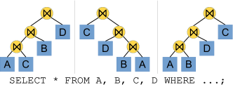
Figure 1: Three different join orderings

Framework Overview Next, we formulate the join order enumeration process as a reinforcement learning problem. Each query sent to the optimizer (and to ReJOIN) represents an episode, and ReJOIN learns over multiple episodes (i.e., continuously learning as queries are sent). Each state will represent subtrees of a binary join tree, in addition to information about query join and selection predicates. Each action will represent combining two subtrees together into a single tree. Note that a subtree can represent either an input relation or a join between subtrees. The episode ends when all input relations are joined (a terminal state). At this point, ReJOIN assigns a reward to the final output join ordering based on the optimizer’s cost model. The final join ordering is then dispatched to the optimizer to perform operator selection, index selection, etc., and the final physical plan is executed by the DBMS.

The framework of ReJOIN is shown in Figure 2. Formally, given a query $q$ accessing relations $r_{1},r_{2},\dots,r_{n}$, we define the initial state of the episode for $q$ as $s_{1}=\{r_{1},r_{2},\dots,r_{n}\}$. This state is expressed as a state vector. This state vector is fed through a neural network [14], which produces a probability distribution over potential actions. The action set $\mathscr{A}_{i}$ for any state is every unique ordered pair of integers from $1$ to $|s_{i}|$, inclusive: $\mathscr{A}_{i}=\left[1,|s_{i}|\right]\times\left[1,|s_{i}|\right]$. The action $(x,y)\in\mathscr{A}_{i}$ represents joining the $x$th and $y$th elements of $s_{i}$ together. An action (i.e., a new join) is selected, and sent back to the environment which transitions to a new state. The state $s_{i+1}$ after selecting the action $(x,y)$ is $s_{i+1}=\left(s_{i}-\{s_{i}[x],s_{i}[y]\}\right)\cup\{s_{i}[x]\bowtie s_{i}[y]\}$. The new state is fed into the neural network. The reward for every non-terminal state (a partial ordering) is zero, and the reward for an action arriving at a terminal state $s_{f}$ (a complete ordering) is the reciprocal of the cost of the join tree $t$, $\mathscr{M}(t)$, represented by $s_{f}$, $\frac{1}{\mathscr{M}(t)}$. Periodically, the agent uses its experience to tweak the weights of the neural network, aiming to earn larger rewards.

Example

Figure 3 shows a potential episode for a query involving four relations: $A$, $B$, $C$, and $D$ The initial state is $s_{1}=\{A,B,C,D\}$. The action set $\mathscr{A}_{1}$ contains one element for each ordered pair of relations, e.g. $(1,4)\in\mathscr{A}_{1}$ represents joining $A$ with $D$, and $(2,3)\in\mathscr{A}_{1}$ represents joining $B$ with $C$. The agent chooses the action $(1,3)$, representing the choice to join $A$ and $C$. The next state is $s_{2}=\{A\bowtie C,B,D\}$. The agent next chooses the action $(2,3)$, representing the choice to join $B$ and $D$. The next state is $s_{3}=\{A\bowtie C,B\bowtie D\}$. At this point, the agent has only two possible choices, $\mathscr{A}_{3}=\{(1,2),(2,1)\}$. Supposing that the agent selects the action $(1,2)$, the next state $s_{4}=\{(A\bowtie C)\bowtie(B\bowtie D)\}$ represents a terminal state. At this point, the agent would receive a reward based on the cost model’s evaluation of the final join ordering.

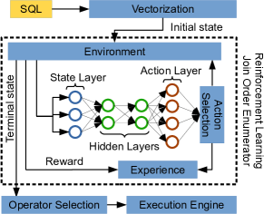
Figure 2: The ReJOIN Framework

2.1 State Vectors

ReJOIN uses a vector representation of each state that captures information about the join ordering (i.e., the binary tree structure) and the join/selection predicates. Next, we outline a simple vectorization strategy which captures this information and demonstrates that reinforcement learning strategies can be effective even with simple input data.

Tree Structure To capture tree structure data, we encode each binary subtree (i.e., join ordering decided so far) $x\in s_{j}$ as a row vector $v$ of size $n$, where $n$ is the total number of relations in the database. The value $v_{i}$ is zero if the $i$th relation is not in $x$, and equal to $\frac{1}{h(i,x)}$ otherwise, where $h(i,x)$ is the height of the relation $r_{i}$ in the subtree $x$ (the distance from the root). In the example in Figure 3, the first row of the tree vector for the second to last state, $\{A\bowtie C,B\bowtie D\}$, corresponds to $(A\bowtie C)$. The third column of the first row has a value of $\frac{1}{2}$, corresponding to $C$ having a height of 2 in the subtree. The second column of the first row has a value of zero since the relation $B$ is not included in the subtree.

Join Predicates

To capture critical information about join predicates, we create an $n\times n$ binary symmetric matrix $m$ for each episode. The value $m_{i,j}$ is one if there is a join predicate connecting the $i$th and the $j$th relation, and a zero otherwise. This simple representation captures feasible equi-joins operations. Figure 3 shows an example of such a matrix $m$. The value $m_{2,1}=m_{1,2}=1$ because of the predicate A.id = B.id. The value $m_{2,3}=m_{3,2}=0$ because there is no join predicate connecting $B$ and $C$.

Selection Predicates The selection predicate vector is a $k$-dimensional vector, where $k$ is the total number of attributes in the database (the total number of attributes across all relations). The $i$th value is one when the $i$th attribute has a selection predicate in the given query, and zero otherwise. This does reveal which attributes are not used to filter out tuples. For example, in Figure 3 the value corresponding to B.a2 is one because of the predicate B.a2 > 100.

2.2 Reinforcement Learning

Policy gradient

Our framework relies on policy gradient methods [19], one particular subset of reinforcement learning. Policy gradient reinforcement learning agents select actions based on a parameterized policy $\pi_{\theta}$, where $\theta$ is a vector that represents the policy parameters. Given a state $s_{t}$ and an action set $\mathscr{A}_{t}$, the policy $\pi_{\theta}$ outputs a score for each action in $\mathscr{A}_{t}$ (in our context, a score for combining two join subtrees). Actions are then selected using various methods [5].

Reinforcement learning aims to optimize the policy $\pi_{\theta}$ over episodes, i.e., to identify the policy parameters $\theta$ that optimizes the expected reward $J_{\pi}(\theta)$. However, the reward $J_{\pi}(\theta)$ is typically not feasible to precisely compute and hence policy gradient methods search for the optimal policy parameters $\theta$ by constructing an estimator $E$ of the gradient of the reward: $E(\theta)\approx\nabla_{\theta}J_{\pi}(\theta)$.

Given an estimate $E$, gradient ascent methods tune the initial random parameters $\theta$ by incrementing each parameter in $\theta_{i}$ by a small value when the gradient $\nabla_{\theta_{i}}J_{\pi}(\theta)$ is positive (the positive gradient indicates that a larger value of $\theta_{i}$ will increase the reward), and decrementing the parameters in $\theta_{i}$ by a small value when the gradient is negative.

Policy gradient deep learning

Policy gradient deep learning methods (e.g.,  [15]) represent the policy $\pi_{\theta}$ as a neural network, where $\theta$ is the network weights, thus enabling the efficient differentiation of $\pi_{\theta}$ [14]. Figure 2 shows the policy network we used in ReJOIN. A vectorized representation of the current state is fed into the state layer, where each value is transformed and sent to the first hidden layer. The first hidden layer transforms and passes its data to the second hidden layer, which passes data to the final action layer. Each neuron in the action layer represents one potential action, and their outputs are normalized to form a probability distribution. The policy $\pi_{\theta}(s_{i},A_{i})$ selects actions by sampling from this probability distribution, which balances exploration and exploitation [19].

The policy gradient $\nabla_{\theta}J_{\pi}(\theta)$ is estimated using samples of previous episodes (queries). Each time an episode is completed (a join ordering for a given query is selected), the ReJOIN agent records a new observation $(\theta,r)$. Here, $\theta$ represents the policy parameters used for that episode and the final cost (reward) $r$ received. Given a set of experiences over multiple episodes $X=\{(\theta^{0},r^{0}),(\theta^{1},r^{1}),\dots,(\theta^{2},r^{2})\}$, various advanced techniques can be used to estimate the gradient $E(\theta)$ of the expected reward [18, 15].

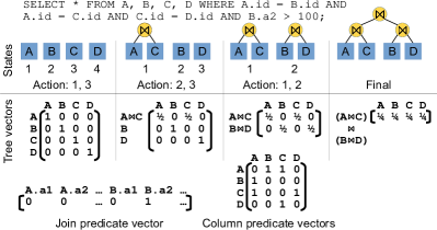
Figure 3: Two possible join order selection episodes

3 Preliminary Results

Here, we present preliminary experiments that indicate that ReJOIN can generate join ordering with cost and latency as good (and often better) as the ones generated from the PostgreSQL [1] optimizer.

Figure 4: ReJOIN Convergence

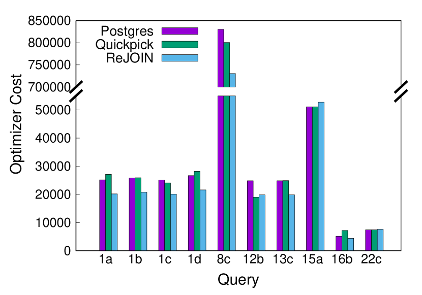
(a) Cost of join orderings

(b) Latency of generated plans

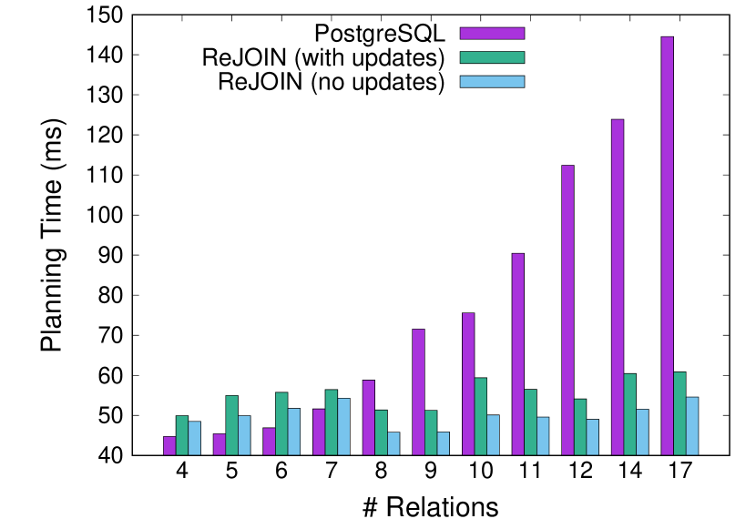
(c) Optimization time

Figure 5: Effectiveness and efficiency results

Our experiments are based on the Join Order Benchmark (JOB), a set of queries used in previous assessments of query optimizers [11]. The benchmark includes a set of 113 query instances of 33 query templates over the freely-available IMDB dataset. We have created a virtual machine pre-loaded with the dataset [3]. Each query joins between 4 and 17 relations, and the two largest relations contain 36M and 15M rows. ReJOIN is trained on 103 queries and tested on 10 queries. Our testing query set includes all instances of one randomly selected query template (template #1), in addition to six other randomly selected queries.

The total database size was 11GB (all primary and foreign keys are indexed) using PostgreSQL [1] on a virtual machine with 2 cores, 4GB of RAM and a maximum shared buffer pool size of 1GB. We configured PostgreSQL to execute the join ordering generated by ReJOIN instead of using its own join enumerator [2].

ReJOIN uses the Proximal Policy Optimization (PPO) algorithm [15], an off-the-shelf [13] state-of-the-art DRL technique. We used two hidden layers with 128 rectified linear units (ReLUs) [7] each.

Learning Convergence

To evaluate its learning convergence, we ran the ReJOIN algorithm repeatedly, selecting a random query from the training set at the start of each episode. The results are shown in Figure 4. The x-axis shows the number of queries (episodes) the ReJOIN agent has learned from so far, and the y-axis shows the cost of the generated plan relative to the plan generated by the PostgreSQL optimizer, e.g. a value of 200% represents a plan with double the cost of the plan selected by the PostgreSQL optimizer. ReJOIN starts with no information, and thus initially perform very poorly. As the number of observed episodes (queries) increases, the performance of the algorithm improves. At around 8,000 observed queries, ReJOIN begins to find plans with lower predicted cost than the PostgreSQL optimizer. After 10,000 queries, the average cost of a plan generated by ReJOIN is 80% of the cost of a plan generated by PostgreSQL. This demonstrates that, with enough training, ReJOIN can learn to produce effective join orderings.

Join Enumeration Effectiveness

To evaluate the effectiveness of the join orderings produced by ReJOIN, we first trained our system over 10,000 queries randomly selected from our 103 training queries (the process took about 3 hours). Then, we used the generated model to produce a join ordering for our 10 test queries. For each test query, we used the converged model to generate a join ordering, but we did not update the model (i.e., the model did not get to add any information about the test queries to its experience set). We recorded the cost (according to the PostgreSQL cost model) of the plans resulting from these test join orderings as well as their execution times. We compare the effectiveness of ReJOIN with PostgreSQL as well as Quickpick [17], which heuristically samples 100 semi-random join orderings and selects the join ordering which, when given to the DBMS cost model, results in the lowest-cost plan.

Optimizer costs We first evaluated the join orderings produced by the ReJOIN enumerator based on the cost model’s assessment. The costs of the plans generated by PostgreSQL’s default enumeration process, Quickpick, and ReJOIN on the 10 test queries are shown in Figure 5(a). “Query XY” on the x-axis refers to the instance Y of the template X in the JOB benchmark. On average, ReJOIN produced join orderings that resulted in query plans that were 20% cheaper than the PostgreSQL optimizer. In the worst case, ReJOIN produced a cost only 2% higher than the PostgreSQL optimizer (Query 15a). This shows that ReJOIN was able to learn a generalizable join order enumeration strategy which outperforms or matches the cost of the join ordering produced by the PostgreSQL optimizer. The relatively poorer performance of Quickpick demonstrates that ReJOIN’s good performance is not due to random chance.

Query latency Figure 5(b) shows the latency of the executed query plans created by Quickpick and ReJOIN relative to the performance of the plan selected by the PostgreSQL optimizer. Here, each test query is executed 10 times with a cold cache. The graph shows the minimum, maximum, and median latency improvement. In every case, the plans produced by ReJOIN’s join ordering outperform or matches the plan produced by PostgreSQL. Hence, ReJOIN can produce plans with a lower execution time (not just a lower cost according to the cost model). Again, the relatively poorer performance of Quickpick demonstrates that ReJOIN is not simply guessing a random join ordering.

Join Enumeration Efficiency

A commonly-voiced opinion about neural networks – and machine learning in general – is that they require operations that are too expensive to include in database internals. Here, we demonstrate that approaches like ReJOIN can actually decrease query planning time. Figure 5(c) shows the average total query optimization time for the 103 queries in the training set, grouped by the number of relations to be joined. We include the planning time for ReJOIN with and without policy updates.

Planning latency For PostgreSQL, as expected, more relations in the query resulted in higher optimization time, as more join orderings need to be considered and ran through the cost model. However, ReJOIN can apply its model in time linear to the number of relations: at each round, two subtrees are joined until a complete join ordering is produced. As a result, while PostgreSQL’s query optimization time increases worse-than-linearly, the query optimization time for ReJOIN is (relatively) flat.

Policy update overhead The additional overhead of performing policy updates per-episode using PPO is relatively small, e.g. $<12ms$. However, once the ReJOIN model is sufficiently converged, policy updates can be skipped to reduce query planning times by an additional 10% to 30%, achieving even shorter query planning times.

4 Open challenges & ongoing work

Our simple reinforcement learning approach to join enumeration indicates that there is room for advancement in the space of applying deep reinforcement learning algorithms to query optimization problems. Overall, we believe the ReJOIN opens up exciting new research paths, some of which we highlight next.

Latency optimization

Cost models depend on cardinality estimates, which are often error-prone. It would be desirable to use the actual latency of an execution plan, as opposed to a cost model’s estimation, as a reward signal. ReJOIN uses the cost model as a proxy for query performance because it enables us to quickly train the algorithm for a large number of episodes – executing query plans, especially the poor ones generated in early episodes, would be overly time-consuming. We are currently investigating techniques [9] to “bootstrap” the learning process by first observing an expert system (e.g., the Postgres query optimizer), mimicking it, and then improving on the mimicked strategy.

End-to-end optimization

ReJOIN only handles join order selection, and requires an optimizer to select operators, choose indexes, coalesce predicates, etc. One could begin expanding ReJOIN to handle these concerns by modifying the action space to include operator-level decisions.

References

- [1] PostgreSQL database, http://www.postgresql.org/.
- [2] PostgreSQL Documentation, ”Controlling the Planner with Explicit JOIN Clauses”, https://www.postgresql.org/docs/10/static/explicit-joins.html.
- [3] Premade VM for replication, http://git.io/imdb.
- [4] SQL Server, https://microsoft.com/sql-server/.
- [5] Arulkumaran, K., et al. A Brief Survey of Deep Reinforcement Learning. IEEE Signal Processing ’17.
- [6] Babcock, B., et al. Towards a Robust Query Optimizer. In SIGMOD ’05.
- [7] Glorot, X., et al. Deep Sparse Rectifier Neural Networks. In PMLR ’11.
- [8] Graefe, G., et al. The Volcano Optimizer Generator. In ICDE ’93.
- [9] Hester, T., et al. Deep Q-learning from Demonstrations. In AAAI ’18.
- [10] Lamb, A., et al. The Vertica Analytic Database: C-store 7 Years Later. VLDB ’12.
- [11] Leis, V., et al. How Good Are Query Optimizers, Really? VLDB ’15.
- [12] Ono, K., et al. Measuring the Complexity of Join Enumeration. In VLDB ’90.
- [13] Schaarschmidt, M., et al. TensorForce: A TensorFlow library for applied reinforcement learning. https://github.com/reinforceio/tensorforce.
- [14] Schmidhuber, J. Deep learning in neural networks. NN ’15.
- [15] Schulman, J., et al. Proximal Policy Optimization Algorithms. arXiv ’17.
- [16] Selinger, P. G., et al. Access Path Selection in a Relational Database Management System. In SIGMOD ’89.
- [17] Waas, F., et al. Join Order Selection (Good Enough Is Easy). In British National Conference on Databases ’10.
- [18] Wang, Z., et al. Sample Efficient Actor-Critic with Experience Replay. ICLR ’17.
- [19] Williams, R. J. Simple statistical gradient-following algorithms for connectionist reinforcement learning. In Machine Learning ’92.