Geometric quench and nonequilibrium dynamics of fractional quantum Hall states

Abstract

We introduce a quench of the geometry of Landau level orbitals as a probe of nonequilibrium dynamics of fractional quantum Hall (FQH) states. We show that such geometric quenches induce coherent many-body dynamics of neutral degrees of freedom of FQH fluids. The simplest case of mass anisotropy quench can be experimentally implemented as a sudden tilt of the magnetic field, and the resulting dynamics reduces to the harmonic motion of the spin-2 “graviton” mode, i.e., the long wavelength limit of the Girvin-MacDonald-Platzman magnetoroton. We derive an analytical description of the graviton dynamics using the bimetric theory of FQH states, and find agreement with exact numerical simulations at short times. We show that certain types of geometric quenches excite higher-spin collective modes, thus establishing their existence in a microscopic model and motivating an extension of geometric theories of FQH states.

I Introduction

Fractional quantum Hall (FQH) states are an epitome of topological phases of matter, featuring exotic phenomena such as fractionalization Laughlin (1983), topological order Wen (1990), and protected edge excitations Halperin (1982); Wen (1991). These phenomena arise as emergent properties of a two-dimensional (2D) electron system in a perpendicular magnetic field Prange and Girvin (1987). As a consequence of Landau level quantization, electrons in these systems have negligible kinetic energy, which paves the way for Coulomb interaction to produce a variety of exotic effects, whose experimental hallmark is the fractional quantization of the Hall conductance Tsui et al. (1982).

Given the intricate, purely interacting nature of FQH states, it comes as no surprise that the existing research mainly focused on their equilibrium (static) properties at zero temperature. These properties have often been described using two closely related frameworks: trial wave functions Laughlin (1983); Jain (1989); Moore and Read (1991); Read and Rezayi (1999) and topological quantum field theory (TQFT) Zhang et al. (1989), which encode the linear response functions Wen and Zee (1992a); Gromov et al. (2015), exotic quasiparticles (“anyons”) Leinaas and Myrheim (1977); Wilczek (1982) characterized by the fractional charge, spin and statistics Wen and Zee (1992b), robust edge modes Wen (1991) and the topological degeneracy on a torus Haldane and Rezayi (1985a); Wen (1990). The predictions of microscopic trial states and TQFT have been tested in numerical simulations of unprecedented accuracy, in particular in the case of Laughlin Laughlin (1983); Haldane and Rezayi (1985b) and composite fermion states Jain (2007).

Besides the low-energy properties, the complete understanding of a quantum system requires the understanding of its dynamics, which is determined by the system’s excited states (possibly at non-zero energy density). This dynamics can be physically probed using the global quantum quench: prepare the system in its ground state $|\psi_{0}\rangle$; abruptly change the Hamiltonian, $H\to H^{\prime}$; let the system evolve and perform measurements on the time-evolved state. For systems that are intrinsically decoupled from the environment, this quench amounts to the innocuous-looking Schrödinger evolution, $|\psi(t)\rangle=\exp(-iH^{\prime}t)|\psi_{0}\rangle$, where $|\psi_{0}\rangle$, crucially, is not an eigenstate of the quench Hamiltonian, $H^{\prime}$. Even though the Schrödinger evolution can be written in such a compact way, it can nevertheless produce incredibly complex outcomes as it might involve highly excited eigenstates of $H^{\prime}$. In one-dimensional integrable systems, where such eigenstates can be computed using techniques like algebraic Bethe ansatz, a particularly deep theoretical understanding of quenches has been achieved (see the recent review Essler and Fagotti (2016)) and verified in cold atom experiments Kinoshita et al. (2006). Other notable examples include one-dimensional critical systems where conformal invariance allows one to analytically describe the post-quench dynamics of various observables (see Ref. Calabrese and Cardy (2016) and references therein) and their holographic duals Nozaki et al. (2013), where quantum quench is interpreted as a process of black hole formation and decay.

In this work, we introduce a new type of geometric quench to study the dynamics of FQH states out of equilibrium. While in integrable systems the term “geometric quench” refers to a sudden change of the size of system Heidrich-Meisner et al. (2008); Buljan et al. (2008); Mossel et al. (2010); Alba and Heidrich-Meisner (2014) (e.g., controlled by the trap potential in cold atomic systems), our setup assumes that the size of the system remains fixed, but the geometry of Landau level orbitals undergoes an abrupt change. This way of probing the system is quite physical: changing the geometry of Landau level orbitals can be achieved directly by tilting the magnetic field, i.e., by introducing a component of magnetic field tangential to the plane occupied by the particles. The tilted field technique is regularly employed in FQH experiments to measure the spin polarization of various states Eisenstein et al. (1988), while more recently it has also been used to map out the anisotropy of the composite fermion Fermi surface Kamburov et al. (2013).

Geometric quench is designed to excite the neutral degrees of freedom of FQH states, which have certain universal features that are geometric in nature. Two major examples are the geometric response function known as Hall viscosity Avron et al. (1995); Read (2009); Haldane and the geometric degrees of freedom responsible for the nematic transition Maciejko et al. (2013); You et al. (2014). The former can be understood in terms of response to the variations of ambient geometry Ferrari and Klevtsov (2014); Abanov and Gromov (2014); Douglas and Klevtsov (2009); Gromov et al. (2015); Bradlyn and Read (2015); Can et al. (2014); Klevtsov and Wiegmann (2015); Hughes et al. (2011); Gromov and Abanov (2014), while the latter can be formulated as fluctuating geometry Haldane (2011); Gromov and Son (2017) (see also Ref. Wiegmann (2018) for a related perspective). We will show that the real-time dynamics following the geometric quench is accurately described by the excitations of geometric degrees of freedom that characterize the underlying FQH states Haldane (2011).

More specifically, in the case of Laughlin states, we will show that a (adiabatic) geometric quench driven by an abrupt change of the effective mass tensor of particles excites a single degree of freedom that carries angular momentum (or spin) $L=2$, which can be viewed as a fluctuating, “intrinsic metric” Haldane . This spin-$2$ degree of freedom is described by a symmetric matrix, which makes it formally similar to the fluctuating space-time metric — a variable that one would like to use in a theory of quantum gravity. For the lack of a better term we will continue to refer to this geometric degree of freedom as “graviton” Yang et al. (2012a); Golkar et al. (2016a). The geometric quench thus allows to excite the emergent FQH graviton and to observe its non-trivial dynamics in time. One has to bear in mind that the graviton discussed in this paper is non-relativistic and massive (i.e., gapped). The closest relativistic cousin of the geometric aspects of the FQH problem is the zwei-dreibein theory of $3$D massive gravity Bergshoeff et al. (2013) (see also Ref. Bergshoeff et al. (2018)).

In order to model the geometric quench, we utilize two recent advances in the theory of the FQH effect: the formulation of the bimetric theory Gromov and Son (2017); Nguyen et al. , which describes topological properties of FQH states on curved surfaces whilst incorporating the mentioned spin-$2$ excitation, and the generalization of the Haldane pseudopotentials Yang et al. (2017a) to systems with broken rotational invariance. Bootstrapping these methods, we derive an analytical description of the real-time dynamics of FQH states following a geometric quench, and confirm it against numerical simulations for the case of Laughlin states.

Our main findings are the following: (i) we demonstrate that geometric quench induces the dynamics of neutral degrees of freedom in FQH states which have geometric character; (ii) in the simplest type of quenches, which are driven by a mass tensor deformation in the Laughlin phase, we show that the post-quench dynamics is determined by an exponentially small fraction of excited states with quadrupolar order (i.e., spin-$2$) in the continuum of the spectrum, whose energy sets the oscillation frequency; (iii) we generalize the bimetric theory Gromov and Son (2017) to describe a quench, and obtain an analytical description of the dynamics following the quench [Eqs. (19) and (20)]; (iv) we show that this analytical description is in excellent agreement with exact numerical simulations of geometric quench in (ii) for finite systems at short times, and generally captures well the oscillations in the dynamics at moderate times, thus justifying the validity of bimetric theory; (v) we design more complex types of geometric quenches which excite the higher-spin excitations in the spectrum of FQH states. We note that higher-spin symmetry has attracted much interest in various areas of theoretical physics, including phase space Fermi fluid Dhar et al. (1992), collective field theory Jevicki and Sakita (1993), generalization of gauge/gravity dualities Giombi et al. (2014), dynamics of incompressible, inviscid fluids Goldin et al. (1987); Arnold and Khesin (1992), large $N$ gauge theory Bars (1990), etc. The presence of higher spin excitations in FQH states, here unambiguously identified via their distinct dynamical response, reveals a much richer structure in FQH states, including the simplest Laughlin states, and calls for an extension of their geometric description Haldane (2011).

The remainder of the paper is organized as follows. In Sec. II, we motivate the geometric quench and provide details of its setup. In Sec. III, we introduce our method, and show that generalized pseudopotentials allow us to identify states that contribute to the quench dynamics. Section IV contains the bulk of our numerical results for the simplest type of quench driven by changing the metric of Landau level orbitals. An analytical description of such quenches is developed in Sec. V in the framework of the bimetric theory. In Sec. VI, we provide an example of a more complex type of quench which excites higher-spin modes in the spectrum, which currently lacks a theoretical description. Our conclusions are presented in Sec. VII, while Appendixes contain additional data and extensions of our results to more realistic (non-instantaneous) quenches and lattice models of fractional Chern insulators.

II Geometric quench of a fractional quantum Hall state

The Hamiltonian describing an FQH system is given by Prange and Girvin (1987)

$$H=\frac{1}{N_{\Phi}}\sum_{\mathbf{q}}\bar{V}_{\mathbf{q}}\bar{\rho}_{\mathbf{q}}\bar{\rho}_{-\mathbf{q}},$$ (1)

where the sum runs over the 2D Brillouin zone (threaded by $N_{\Phi}$ flux quanta) and $\bar{\rho}_{\mathbf{q}}=\sum_{j=1}^{N}e^{i\mathbf{q}\cdot\mathbf{R}_{j}}$ is the density operator projected to a single Landau level (LL). The projection to a LL imposes the non-commutative geometry of the “guiding center coordinates,” $\left[R_{i}^{a},R_{j}^{b}\right]=-i\ell_{B}^{2}\epsilon^{ab}\delta_{i,j}$, where $\ell_{B}=\sqrt{\hbar/eB}$ is the magnetic length Prange and Girvin (1987). This non-trivial constraint, along with the absence of kinetic energy in Eq. (1), gives rise to a wide variety of ordered phases, depending on the filling factor $\nu=N/N_{\Phi}$ and the details of the (projected) interaction potential $\bar{V}_{\mathbf{q}}$. Note that because the guiding centers do not commute, bosonic FQH states are also possible and realize a similar variety of phases Cooper et al. (2001); Regnault and Jolicoeur (2003). In this paper, we focus on the simplest Laughlin states, which occur at filling $\nu=1/2$ for bosons and $\nu=1/3$ for fermions.

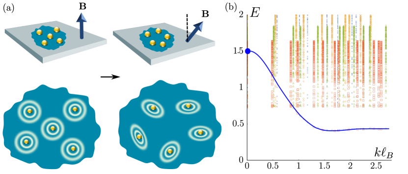
Figure 1: (a) Geometric quench protocol: instantaneous tilt of the magnetic field induces dynamics of the intrinsic metric, which describes the shape of particle-flux composites that form an FQH state. (b) The excitation spectrum of the $\nu=1/3$ Laughlin state, obtained by exact diagonalization of its $V_{1}$ parent Hamiltonian, in systems with $N=7-10$ electrons. Blue line traces out the SMA collective mode Girvin et al. (1985), which transforms into an emergent graviton excitation in the $k\to 0$ limit (around energy $E\approx 1.5$). It will be shown in Sec. V that geometric quench induces oscillatory dynamics of the $k\to 0$ limit of the graviton mode. Note that this mode is formed by excited states in the continuum of the energy spectrum.

Beside the non-commutative constraint, geometry appears in an FQH problem in three distinct guises. First, the interaction potential $\bar{V}_{\mathbf{q}}=V_{\mathbf{q}}|F_{m}(\mathbf{q})|^{2}$ is a function of two independent tensors $g_{m}$ and $g_{i}$ Haldane (2011), where $F_{m}(\mathbf{q})=\exp(-g_{m}^{ab}q_{a}q_{b}\ell_{B}^{2}/4)$ is the (lowest) LL form factor and $V_{\mathbf{q}}$ in general depends on $\sqrt{g_{i}^{ab}q_{a}q_{b}}$ (for the Coulomb interaction, $V_{\mathbf{q}}=2\pi/\sqrt{g_{i}^{ab}q_{a}q_{b}}$). These two tensors are imposed by extrinsic experimental conditions, such as the direction of the magnetic field and properties of the underlying solid-state material. $g_{m}$ has physical origin in the band mass tensor and can be conveniently parametrized by a $2\times 2$ unimodular matrix (${\rm det}g_{m}=1$)

$$g_{m}=\left(\begin{array}[]{cc}\cosh Q+\cos\phi\sinh Q&\sin\phi\sinh Q\\ \sin\phi\sinh Q&\cosh Q-\cos\phi\sinh Q\\ \end{array}\right),\;\;\;\;\;$$ (4)

where $Q$ and $\phi$ are real numbers that parametrize a stretch or rotation of the tensor. On the other hand, $g_{i}$ is in general different from $g_{m}$. In the case of Coulomb interaction, $g_{i}$ originates from the dielectric tensor of the material that hosts the FQH system. Note that both $g_{m}$ and $g_{i}$ define the shape of a circle: $g_{m}$ enters the single-particle wave function thus defining the shape of LL orbitals, while $g_{i}$ determines the shape of the interaction equipotentials. They hence effectively measure the distance from the “circle center,” and in this sense we alternatively refer to them as extrinsic metrics Haldane (2011).

Subject to these two extrinsic metrics, an FQH state develops a third, intrinsic geometric degree of freedom. As a many-body property of the system, this intrinsic degree of freedom defines the shape of particle-flux composite droplets in FQH ground states and can also be thought of as a metric $\hat{g}$ parametrized by the same matrix as in Eq. (4). If the extrinsic metrics are equal ($g_{m}=g_{i}$), but not necessarily isotropic ($\neq{\hbox{1\kern-1.49994pt\vrule width=0.8pt,depth=-0.5pt}}$), the intrinsic metric is equal to them ($\hat{g}=g_{m}=g_{i}$) and the physical state is isotropic in a transformed coordinate frame. More generally, when $g_{m}\neq g_{i}$, $\hat{g}$ is determined from energetic compromise between $g_{m}$ and $g_{i}$, and is in general different from both of them Yang et al. (2012b); Wang et al. (2012a). The intrinsic metric, as an emergent many-body property of the system, will be the main focus of the quench dynamics in this paper.

The dynamics of $\hat{g}$ can in principle be induced by changing the mass tensor $g_{m}$. While this might be feasible in materials such as AlAs Gokmen et al. (2010), a much more practical way is to tilt the magnetic field [Fig. 1(a)]. Semiclassically, the particles still prefer to make circular orbits around the tilted direction, but because they are confined to a narrow sample, their orbits deform into ellipses in the plane of the FQH system, hence giving rise to an effective mass anisotropy. In fact, assuming a parabolic confining potential in the perpendicular direction, tilt can be exactly represented as a $2\times 2$ anisotropic mass tensor Yang et al. (2012b); Papić (2013); Yang et al. (2017b). Hence, to an excellent approximation, we can model the effect of a tilt by an anisotropic mass tensor like in Eq. (4) Papić (2013).

Our quench protocol can now be defined as follows: (i) prepare a Laughlin state $|\psi_{0}\rangle$ as the ground state of $H$ with mass tensor $g_{m}$; (ii) instantaneously change $g_{m}\to g_{m}^{\prime}$; (iii) evolve in time assuming the system is closed, i.e., $|\psi(t)\rangle=\exp(-iH^{\prime}t)|\psi_{0}\rangle$, and measure the intrinsic metric as a function of time, $\hat{g}(t)$. This protocol is the minimal theoretical model for an experiment where the magnetic field is suddenly tilted. At considerable computational expense, the model can be made more realistic by directly including a parallel field (instead of approximating it by mass anisotropy), relaxing the assumption of a closed system, etc. In later sections of the paper, we will consider some generalizations of the protocol where the quench cannot be described in terms of a $2\times 2$ metric (Sec. VI) or when it is not applied instantaneously (Appendix C).

The intuition behind the geometric quench is the following. In a purely perpendicular field, an FQH state is a low-entangled state of composite objects – particles surrounded by correlation holes of certain size. For example, in the $\nu=1/3$ Laughlin state, we can view them as electrons in an area corresponding to three magnetic flux quanta [Fig. 1(a)]. These objects have a finite area (fixed by the electron density and total flux through the system), but their shape can vary and is determined by the intrinsic metric $\hat{g}$ of the FQH state Johri et al. (2016), or equivalently by two real parameters, $Q$ and $\phi$, as in Eq. (4). For a adiabatic quench that keeps the system within the Laughlin phase, these droplets are expected to fluctuate and our goal is to determine the equations of motion for $Q$ and $\phi$. This is, however, a non-trivial problem because the representation of a state in Fig. 1(a) is merely a cartoon (e.g., the operators projected onto the droplets do not commute with one another).

As emphasized earlier, the key to understanding dynamics are the excited eigenstates in the spectrum of $H^{\prime}$. Such a spectrum for the Laughlin $\nu=1/3$ state, obtained by diagonalization of its parent Hamiltonian – the $V_{1}$ Haldane pseudopotential Haldane (1983)– is shown in Fig. 1(b). The low-energy spectrum is dominated by a collective mode known as the Girvin-MacDonald-Platzman (GMP) mode or “magnetoroton” Girvin et al. (1985, 1986). This mode is accurately described by the single-mode approximation (SMA), and intuitively represents a density modulation on top of the ground state given by $\bar{\rho}_{\mathbf{k}}|\psi_{0}\rangle$. Such SMA trial wavefunctions were shown to give an excellent description of the actual collective excitation for momenta smaller than the magnetoroton minimum Repellin et al. (2014), both for the exact Laughlin state and the Coulomb ground state. Generalizations of the SMA, based on Jack polynomials, have been shown to be microscopically accurate at all values of momenta accessible in finite systems Yang et al. (2012a).

Since the SMA dominates the low-energy physics of an FQH state, it could be expected that it also plays a crucial role in the quench dynamics. However, this becomes less clear if one notices that our quench protocol preserves the translation symmetry of the initial state, hence all dynamics takes place in the $\mathbf{k}=0$ sector of the Hilbert space that contains the uniform Laughlin state. The $k\to 0$ limit of the SMA mode, i.e., the spin-$2$ graviton Yang et al. (2012a), lies inside the 2 quasiparticle-2 quasihole continuum of states [Fig. 1(b)], hence it is far from obvious that quench dynamics can be modelled by this single degree of freedom (although in some cases the $k\to 0$ limit of the SMA mode appears to be below the continuum of the energy spectrum Jolicoeur (2017)). In the following section, we present the results of our exact numerical simulations of the quench dynamics in finite-size systems. These results will show that the simplest type of geometric quench described by Eq. (4), indeed, gives rise to coherent oscillations of the geometric spin-2 degree of freedom for the Laughlin state. We note, however, that more general types of quenches are also possible, which cannot be mapped to a simple modification of the mass tensor. These quenches, which will be considered in Sec. VI, excite the tower of higher spin modes in the spectrum of an FQH state, giving rise to non-trivial dynamics, which is not captured by the simple graviton oscillation.

III Method

We model the quench by performing numerically exact time evolution with the Hamiltonian in Eq. (1) defined for $N$ particles and $N_{\Phi}$ flux quanta on a square torus [Fig. 2(a)]. Magnetic translation symmetry Haldane (1985) is used to reduce the complexity of the calculation and to classify the many-body eigenstates. We focus on the Laughlin states of bosons and fermions, corresponding to filling factors $\nu=1/2$ and $\nu=1/3$, respectively.

We consider two types of interaction potentials. In the first case, we assume a model (short-range) interaction for which the Laughlin state is the unique (and the densest) zero-energy state Haldane (1983). This interaction is a simple contact repulsion for bosons, $V_{\mathbf{q}}=1$, and for fermions it is $V_{\mathbf{q}}=L_{1}(g_{m}^{ab}q_{a}q_{b})$, where $L_{1}$ is the first Laguerre polynomial. As customary in the literature Haldane (2011), in the model interaction, we have assumed that the interaction metric $g_{i}$ coincides with the Landau orbit metric $g_{m}$. In the second case, we consider the Coulomb interaction, for which $g_{i}$ is kept isotropic, i.e., $V_{\mathbf{q}}=2\pi/\sqrt{q_{x}^{2}+q_{y}^{2}}$, but the mass tensor $g_{m}$ is allowed to be non-isotropic.

For both types of interaction, the quench is implemented by switching $g_{m}$ to $g_{m}^{\prime}$ at time $t=0$, where both $g_{m}$ and $g_{m}^{\prime}$, for simplicity, are taken to be diagonal, like in Eq. (15) below. For small system sizes, the subsequent time evolution is performed by obtaining all energy eigenvalues $\epsilon_{n}$ and the corresponding eigenvectors $|n\rangle$ of the quench Hamiltonian $H^{\prime}$, and then evaluating $|\psi(t)\rangle=\sum_{n}\exp(-i\epsilon_{n}t)\langle n|\psi_{0}\rangle|n\rangle$. By restricting the sum to a subset of eigenstates, one can conveniently project the dynamics onto a desired energy shell. At larger system sizes, we use time-dependent Lanczos methods to iteratively compute $|\psi(t)\rangle$.

We use the same parametrization for the intrinsic metric $\hat{g}$ as in Eq. (4). Due to its invariance under $Q\rightarrow-Q$ and $\phi\rightarrow\phi+\pi$, we focus on $Q\geq 0$. For a given state $|\psi(t)\rangle$, $\hat{g}$ is determined by brute force search over a large set of (precomputed) trial states $|\psi_{\rm{trial}}\rangle$, i.e., model Laughlin states parametrized by $Q\in\left[0,Q_{\max}\right]$ and $\phi\in\left[-\pi,\pi\right]$, such that the overlap $|\langle\psi_{\rm{trial}}|\psi(t)\rangle|$ is maximized. For adiabatic quenches, we found it sufficient to restrict to $Q_{\max}=1$ and $\phi\in[-\pi/2,\pi/2]$. The confidence in the result is quantified by the maximum overlap achieved: if this overlap is not close to 1 (like in the case of strong quench), none of the trial states appropriately describes the system and the intrinsic metric should be determined via some other means, for example, via minimization of the total energy or momentum polarization Gromov et al. (2017).

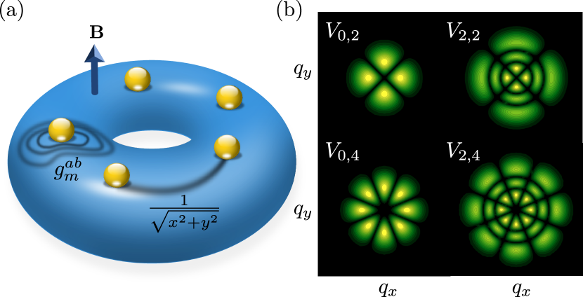
Figure 2: (a) An FQH system on the surface of a torus threaded by a perpendicular magnetic field. The mass tensor $g_{m}$ determines the metric of the Landau level orbitals and is used to drive a quench, while the Coulomb potential is assumed to be isotropic. (b) Contours in momentum space of the leading order anisotropic pseudopotentials for bosons Yang et al. (2017a) with quadrupolar ($V_{0,2}$, $V_{2,2}$) and octupolar ($V_{0,4}$, $V_{2,4}$) structure.

Finally, in order to identify states corresponding to the spin-$n$ excitation, we use the recently developed formalism of anisotropic pseudopotentials Yang et al. (2017a). In Ref. Yang et al. (2017a) it was shown that any two-particle interaction, including cases where metrics $g_{m}$ and $g_{i}$ are different, can be expanded into an orthonormal basis of generalized pseudopotentials. These operators maintain translation invariance, but break rotation symmetry to a discrete subgroup. Up to normalization prefactors, the generalized pseudopotentials are given by Yang et al. (2017a)

$$V_{m,n}\left(g_{p};q_{x},q_{y}\right)=L_{m}^{n}\left(g_{p}^{ab}q_{a}q_{b}\right)\textbf{q}^{n}+{\rm c.c.},$$ (5)

where $m$, $n$ are even integers (for bosons). When $n=0$, these reduce to the usual (isotropic) Haldane pseudopotentials Haldane (1983). $V_{m,n}$ explicitly depends on the metric $g_{p}$ through the argument of the Laguerre polynomial, as well as the vector $\mathbf{q}$. For simplicity, we fix $g_{p}={\hbox{1\kern-1.49994pt\vrule width=0.8pt,depth=-0.5pt}}$ and $\mathbf{q}=\frac{1}{\sqrt{2}}(q_{x}+iq_{y})$ in our numerics.

Contours of leading-order $V_{m,n}$ for bosons are depicted in Fig. 2(b). In particular, we can observe that the dominant pseudopotential $V_{0,2}$ has a clear quadrupolar structure in momentum space, indicating that $\hat{V}_{0,2}$ carries angular momentum $L_{z}=2$. Based on this, we use $\hat{V}_{0,n}$ as a spectroscopic probe to identify many-body eigenstates, which are part of the effective spin-$n$ excitation. To that end, we introduce the following “spectral function”:

$$I_{m,n}(\omega)=\sum_{j}\delta(\omega-\epsilon_{j})|\langle j|\hat{V}_{m,n}|0\rangle|^{2},$$ (6)

where $\epsilon_{j}$ and $|j\rangle$ are the eigen-energy and eigenstate of Eq. (1). This is a generalization of the spectral function that describes an acoustic wave absorption experiment Yang (2016). The peaks of $I_{m,n}$ can be used to obtain the frequencies of different spin modes in the quench dynamics. In the following section, we investigate in detail $I_{0,2}$ and show that it indeed yields the frequency of the graviton mode.

IV Results

Here, we present our numerical results for adiabatic quenches, where the mass tensor is instantaneously changed from $g_{m}={\rm diag}(e^{A_{0}},e^{-A_{0}})$ to $g_{m}^{\prime}={\rm diag}(e^{A_{1}},e^{-A_{1}})$ with $A_{0}$ and $A_{1}$ close to $0$. By “adiabatic” quench we mean that the system remains in the Laughlin phase. Note that this does not imply that we restrict to an infinitesimal variation of the parameters in the Hamiltonian. Indeed, the parameters of our quenched Hamiltonian differ by a finite amount from the original Hamiltonian, which allows the dynamics to explore a finite density of excitations.

In the following, we focus on the dynamics of $\hat{g}$ for $\nu=1/2$ bosons in detail, while similar results for $\nu=1/3$ fermions are given in Appendix D. In all numerical data below, time is given in units of inverse energy [$e^{2}/(\epsilon\ell_{B})$ in the case of Coulomb interaction], with $\hbar=1$.

IV.1 Isotropic-to-anisotropic quench

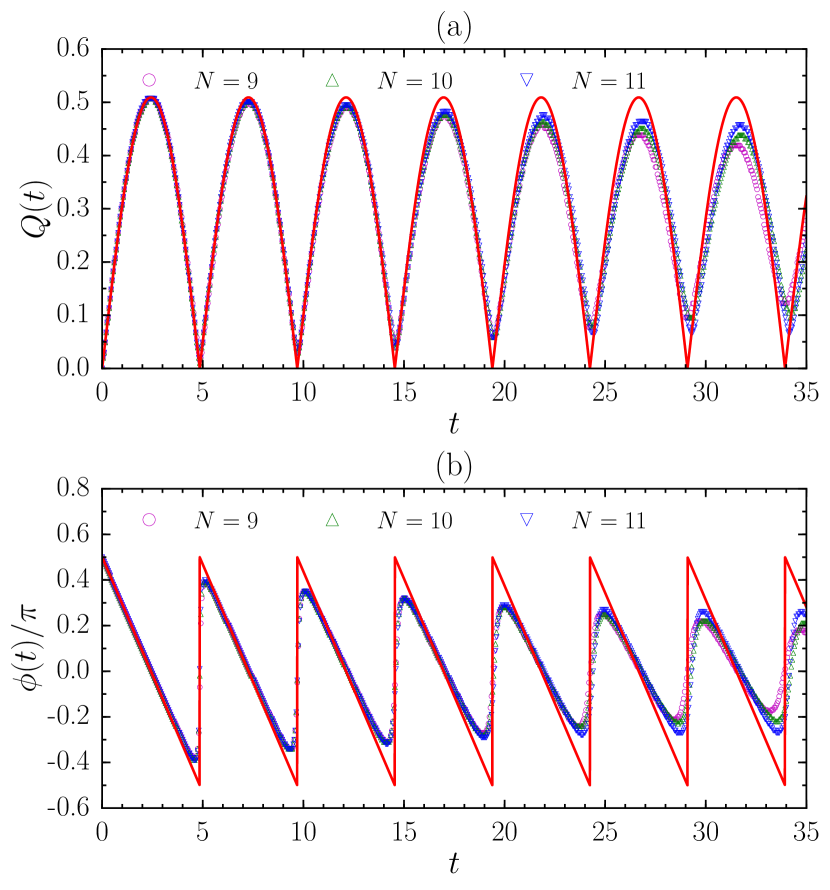
Figure 3: Exact dynamics of (a) $Q$ and (b) $\phi$ for $N=9-11$ bosons at $\nu=1/2$ with the contact interaction. The quench is driven by choosing $A_{0}=0$ and $A_{1}=\ln 1.3$. The red curves are fits to Eqs. (7) and (8), which coincide with the predictions of the bimetric theory, discussed in Sec. V.

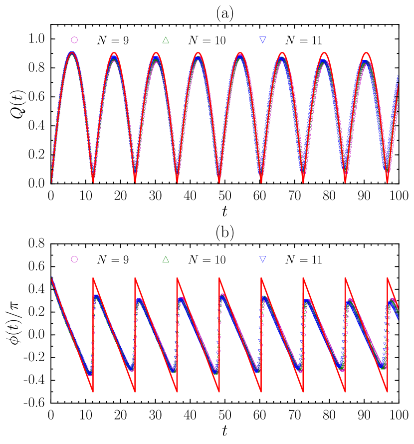
Figure 4: Exact dynamics of (a) $Q$ and (b) $\phi$ for $N=9-11$ bosons at $\nu=1/2$ with the Coulomb interaction. The quench is driven by choosing $A_{0}=0$ and $A_{1}=\ln 2.0$. The red curves are fits to Eqs. (7) and (8), which coincide with the predictions of the bimetric theory, discussed in Sec. V.

We start with the simple case of $A_{0}=0,A_{1}>0$, where the initial state is the isotropic Laughlin state. As representative examples, we choose $A_{1}=\ln 1.3$ and $A_{1}=\ln 2.0$ for quenches driven by contact and Coulomb interactions, respectively. The intrinsic metric $\hat{g}$ of the post-quench state is determined by the maximum of the overlap between the post-quench state and a trial set of anisotropic Laughlin states. The regime of adiabatic quench corresponds to the maximum of this overlap being close to unity. The exact dynamics of $\hat{g}$ up to moderate times is shown in Figs. 3 and 4 for the two types of interactions. We observe that both $Q$ and $\phi$ oscillate with a well-defined frequency (and in particular, $\phi$ appears to be a linear function of time). This is rather surprising because the induced change in the microscopic structure of the FQH state is by no means small: for the above choices of $A_{1}$ in Figs. 3 and 4, we find the maximum anisotropy $e^{Q}$ of the post-quench state to be larger than the initial (isotropic) state by a factor $1.5-2.5$.

Assuming a single harmonic, we might guess that the oscillations in Figs. 3 and 4 are well described by

$$Q(t) = 2A\sin\left(\frac{E_{\gamma}t}{2}\right),\;\;\;\phi(t)=\frac{\pi}{2}-\frac{E_{\gamma}t}{2},$$ (7)

$$Q(t) = -2A\sin\left(\frac{E_{\gamma}t}{2}\right),\;\;\;\phi(t)=\frac{3\pi}{2}-\frac{E_{\gamma}t}{2},$$ (8)

where $Q$ obeys harmonic motion and $\phi$ has a simple linear dependence on time. Note that only one of these two solutions is independent because the system is invariant under $Q\rightarrow-Q$ and $\phi\rightarrow\phi+\pi$. Thus, we can focus on the $Q\geq 0$ part and consider $\phi\;{\rm mod}\;2\pi$. By inspection of $Q(t)$, we see the solution will alternate between the two branches, which doubles the frequency from $E_{\gamma}/2$ to $E_{\gamma}$. The overall prefactor (written as $2A$) is expected to be proportional to the intrinsic anisotropy of the state.

Fitting the first one or two oscillations in Figs. 3 and 4 against Eq. (7) yields a remarkably accurate agreement with the full dynamics across the entire time interval. What sets the frequency, $E_{\gamma}$, of the oscillations? From the fits, we obtain $E_{\gamma}\approx 1.296$ and $0.520$ for the cases of contact and Coulomb interactions, respectively. These values do not match the spectral gap in the $\mathbf{k}=0$ momentum sector, which can be much smaller (see Fig. 1). Instead, as shown below, they agree with the graviton gap very well, which we independently estimate to be $\approx 1.3$ for the contact interaction and $0.52$ for the Coulomb interaction.

In order to justify the identification of $E_{\gamma}$ with the graviton gap, we use $I_{0,2}(\omega)$ spectral function defined in Eq. (6) to detect the states that carry spin-2. We expect peaks of $I_{0,2}(\omega)$ at energies corresponding to the spin-$2$ excitations that comprise the graviton mode. In Fig. 5, we show $I_{0,2}(\omega)$ [normalized by $\int I_{0,2}(\omega)d\omega$] for contact and Coulomb interactions in isotropic systems (similar data are obtained for weakly anisotropic systems). In the case of contact interaction, we observe sharply pronounced peaks of $I_{0,2}(\omega)$ around $\omega=1.3$ for various system sizes [Fig. 5(a)], which means that spin-$2$ eigenstates concentrate in this narrow energy window, corresponding to the graviton gap $E_{\gamma}\approx 1.3$. For Coulomb interacting systems, a pronounced peak in $I_{0,2}(\omega)$ also exists, but at a lower energy $\omega\approx 0.55$ [Fig. 5(b)]. As an independent estimate of the graviton gap, we use the discrete Fourier transform of $Q$ (see insets of Fig. 5). This Fourier transform also shows a sharp peak around the same energy as that in $I_{0,2}(\omega)$, which further confirms that the dynamics of the intrinsic metric is indeed caused by the graviton oscillation.

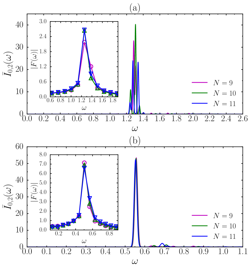
Figure 5: Normalized spectral function ${\bar{I}}_{0,2}(\omega)=I_{0,2}(\omega)/\int I_{0,2}(\omega)d\omega$ for isotropic systems of $N=9-11$ bosons at $\nu=1/2$ with (a) contact and (b) Coulomb interactions. The insets show the discrete Fourier transform $|F(\omega)|$ of $Q$ in Figs. 3 and 4. Markers in insets and curves in main figures with the same color refer to the same system size.

IV.2 States contributing to dynamics

The agreement between the oscillation frequency in the exact dynamics of $\hat{g}$ and the graviton gap strongly implies that the dynamics is dominated by spin-$2$ eigenstates of $H^{\prime}$. We now scrutinize this conjecture by quantifying how well the full dynamics can be reproduced by an explicit projection to the subset of eigenstates centered around the energy of the spin-$2$ mode.

The projected subspace is defined by the eigenstates $|n\rangle$ of $H^{\prime}$ with dominant matrix elements $|\langle n|\hat{V}_{0,2}|0\rangle|^{2}$. The weight of this projection is measured by

$$f=\left(\sum_{n=0}^{M-1}|\langle n|\hat{V}_{0,2}|0\rangle|^{2}\right)/\left(\sum_{n=0}^{D-1}|\langle n|\hat{V}_{0,2}|0\rangle|^{2}\right),$$ (9)

where $|n\rangle$ have been sorted in descending order according to $|\langle n|\hat{V}_{0,2}|0\rangle|^{2}$. Here $M$ is the number of kept states and $D$ is the total number of eigenstates that we can obtain from exact diagonalization of $H^{\prime}$, i.e., $D$ is equal to the Hilbert space dimension in the ${\bf k}=0$ sector for $N\leq 9$, while for practical reasons we kept $D=200$ for larger systems ($N=10-12$). Remarkably, the number of states we need to saturate the total weight $f$ is significantly smaller than the Hilbert space dimension. Fixing $f=99\%$, the finite-size scaling of the required $M$ clearly indicates that only an exponentially small fraction of the whole Hilbert space carries spin-$2$, as seen in Fig. 6.

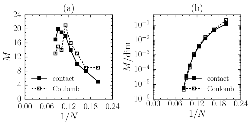
Figure 6: Finite-size scaling of the number of spin-$2$ states in the ${\bf k}=0$ Hilbert space for $N=5-12$ bosons at $\nu=1/2$. $M$ represents the number of states which contain $f=99\%$ of the total $|\langle n|\hat{V}_{0,2}|0\rangle|^{2}$. We consider both contact and Coulomb quench Hamiltonians, with $A_{1}=\ln 1.3$ and $A_{1}=\ln 2.0$, respectively. The plots show (a) $M$ and (b) $M/{\rm dim}$, where ${\rm dim}$ is the ${\bf k}=0$ Hilbert space dimension.

While the exponentially decaying ratio of $M$ to the Hilbert space dimension might not be entirely surprising (since it still does not preclude $M$ being exponentially large in the system size), it can also be shown that, in absolute terms, only a very small number of states $M$ yields a very accurate approximation to the exact dynamics. In Appendix B, we perform the above projection, based on the $|\langle n|\hat{V}_{0,2}|0\rangle|^{2}$ matrix elements, for the dynamics of $N=11$ bosons driven by the isotropic-to-anisotropic quench (Fig. 10). Remarkably, the main features of the exact dynamics are already accurately reproduced for $M$ less than $10$, even if there are as many as $533160$ eigenstates in the entire ${\bf k}=0$ Hilbert space. Such an excellent approximation of the exact dynamics by an exponentially small fraction of states in the Hilbert space is further evidence for the picture of graviton oscillation.

V Adiabatic geometric quench in bimetric theory

In the previous Section, we have established that quenching the mass tensor, Eq. (4), in the Laughlin phase gives rise to dynamics which is supported over a vanishingly small fraction of states that carry spin-2. Thus we expect that our results in Sec. IV can be used to test the validity of the bimetric theory Gromov and Son (2017). Here, we generalize the bimetric theory to anisotropic quantum Hall states, and derive an analytical description of the dynamics of the intrinsic metric $\hat{g}$ after a quench exciting spin-$2$ states. We find that this analytical prediction agrees remarkably well with the exact numerics of geometric quench in Sec. IV, which supports the validity of the bimetric theory. Despite of its agreement with the bimetric theory in special quenches exciting spin-$2$ states, we should emphasize that geometric quench is a logically independent method and contains much new physics beyond the bimetric theory (see Sec. VI).

V.1 Lagrangian for the isotropic case

The bimetric theory describes the gapped dynamics of a single spin-$2$ degree of freedom in an FQH system, interacting with an external electro-magnetic field and ambient geometry. The dynamical degree of freedom is the vielbein $\hat{e}^{\alpha}_{i}$ Carroll (2004) that “squares” to the dynamic, unimodular metric $\hat{g}_{ij}=\hat{e}^{\alpha}_{i}\hat{e}^{\beta}_{j}\delta_{\alpha\beta}$, or simply $\hat{g}=\hat{e}\cdot\hat{e}^{T}$. Here, $\hat{g}$ corresponds to the intrinsic metric of the FQH state mentioned in Sec. II. The inverse metric is given by $\hat{G}^{ij}=\hat{E}_{\alpha}^{i}\hat{E}_{\beta}^{j}\delta^{\alpha\beta}$, where $\hat{E}_{\alpha}^{i}$ is the inverse vielbein Carroll (2004), satisfying $\hat{E}^{i}_{\alpha}\hat{e}_{j}^{\alpha}=\delta^{i}_{j}$. The unimodular condition on $\hat{g}_{ij}$ takes form $\sqrt{g}=\sqrt{\hat{g}}$, where $\sqrt{g}$ is the determinant of the ambient metric $g_{ij}=\delta_{AB}e^{A}_{i}e^{B}_{j}$ and $e^{A}_{i}$ is the ambient vielbein. Thus, in flat ambient space (that is, when $g_{ij}=\delta_{ij}$), $\sqrt{\hat{g}}=1$.

In the absence of an external electric field, and when the magnetic field is homogeneous, the Lagrangian takes the form Gromov and Son (2017)

$$\mathcal{L}=\frac{\nu\varsigma}{2\pi\ell_{B}^{2}}\hat{\omega}_{0}-\frac{m}{2}\left[\frac{1}{2}\hat{g}_{ij}g^{ij}-\gamma\right]^{2}=\mathcal{L}_{\rm top}+\mathcal{L}_{\rm pot}\,,$$ (10)

where $\hat{\omega}_{0}$ is the temporal component of the (dynamic) Levi-Civita spin connection, given by

$$\hat{\omega}_{0}=\frac{1}{2}\epsilon_{\alpha}{}^{\beta}\hat{E}^{i}_{\beta}\partial_{0}\hat{e}_{i}^{\alpha}\,.$$ (11)

The phenomenological coefficient $m$ sets the energy scale that determines the gap of the spin-$2$ mode. The quantized coefficient $\varsigma$ is determined by the “shift” $\mathcal{S}$ Gromov and Son (2017) and takes the value $|\varsigma|=\frac{|\mathcal{S}-1|}{2}$. The phenomenological parameter $\gamma$ is used to tune the theory close to the nematic phase transition, where the SMA is exact, in the gapped phase $\gamma<1$. Further details on the bimetric Rieman-Cartan geometry can be found in Refs. Gromov and Son (2017); Gromov et al. (2017). We will utilize it to introduce anisotropy into the problem.

V.2 Anisotropy in bimetric theory

To introduce the quadrupolar anisotropy from a non-trivial mass tensor or other sources, we take the inspiration from Ref. Gromov et al. (2017), where quadrupolar anisotropy was described in geometric terms. More concretely, we introduce a unimodular matrix $\mathrm{m}_{AB}$, and construct a rank-2 tensor from it according to

$$g^{(\mathrm{m})}_{ij}=\mathrm{m}_{AB}e^{A}_{i}e^{B}_{j}\,,$$ (12)

where $e^{A}_{i}$ are the vielbeins that describe the ambient geometry. We now generalize Eq. (10) to the anisotropic case. To do so, we simply replace $g_{ij}$ by $g^{(\mathrm{m})}_{ij}$ in Eq. (10).

To analyze the theory further, we make the following simplifying assumptions: (i) the ambient space is assumed to be flat, $e^{A}_{i}=\delta^{A}_{i}$, and (ii) we assume a particular parametrization of $g^{(\mathrm{m})}_{ij}$, given by

$$g_{ij}^{(\mathrm{m})}=\left(\begin{array}[]{cc}e^{A}&0\\ 0&e^{-A}\\ \end{array}\right)\,,$$ (15)

where $A$ is a real parameter that defines the effective anisotropy in the FQH system, which is a compromise between two extrinsic metrics $g_{m}$ and $g_{i}$ as discussed in Sec. II. The abrupt change of the mass tensor $g_{m}$ in our quench protocol will lead to the change of $A$ in Eq. (15).

In order to compute the dynamics of $\hat{g}_{ij}$, we parametrize it in terms of $Q$ and $\phi$ as in Eq. (4). Both $Q$ and $\phi$ are functions of time, but not space, since the problem we will consider is homogeneous (i.e., the quench is global). The two terms in the Lagrangian take the form

$$\mathcal{L}_{\rm top} = \frac{\varsigma\bar{\rho}}{2}\left(1-\cosh Q\right)\dot{\phi}\,,$$ (16)

$$\mathcal{L}_{\rm pot} = -\frac{m}{2}\left(\gamma+\sinh A\sinh Q\cos\phi-\cosh A\cosh Q\right)^{2}\;.\;\;\;\;\;\;$$ (17)

The equations of motion are found from

$$\frac{\delta S}{\delta\phi}=0\,,\qquad\frac{\delta S}{\delta Q}=0\,,$$ (18)

where $S=\int d^{3}x\,\mathcal{L}$ is the action. The equation for $\phi(t)$ takes the form

$$\dot{\phi}\sinh Q=-2\Omega\left(\sinh A\cosh Q\cos\phi-\cosh A\sinh Q\right)\left(\gamma+\sinh A\sinh Q\cos\phi-\cosh A\cosh Q\right)\,,$$ (19)

and for $Q(t)$ we find

$$\dot{Q}\sinh Q=-2\Omega\sin\phi\sinh Q\sinh A\left(\gamma+\sinh A\sinh Q\cos\phi-\cosh A\cosh Q\right)\,,$$ (20)

where we have introduced the energy scale $\Omega=\frac{m}{\bar{\rho}\varsigma}$. Equations (19) and (20) are the central result of this section.

V.3 Isotropic limit

In the isotropic case we must take $A\rightarrow 0$. We find

$$\dot{Q}=0\,,\qquad\dot{\phi}=2\Omega\left(\gamma-\cosh Q\right)\,.$$ (21)

Choosing the solution $Q=0$ of the first equation, the second equation reads

$$\dot{\phi}=-2\Omega(1-\gamma)\equiv-E_{\gamma}\,\quad\Rightarrow\quad\phi(t)=\phi(0)-E_{\gamma}t\,,$$ (22)

from where we interpret $E_{\gamma}=2\Omega(1-\gamma)=\frac{2m(1-\gamma)}{\bar{\rho}\varsigma}$ as the gap of the spin-$2$ part of the GMP mode at $\mathbf{k}=0$ Gromov and Son (2017). When $\gamma\rightarrow 1$, the gap closes and the FQH state undergoes a nematic phase transition Gromov and Son (2017). The dynamical metric evaluated on this solution takes the form

$$\hat{g}_{ij}=\left(\begin{array}[]{cc}1&0\\ 0&1\\ \end{array}\right)\,,$$ (23)

consequently the dynamics of $\phi(t)$ is not visible in the fluctuations of the dynamical metric. Formally speaking, this happens because $Q=0$. When $Q$ is different from $0$ the metric will be sensitive to the dynamics of $\phi$. This is what happens in the case of weak anisotropy discussed next.

V.4 Adiabatic geometric quench in bimetric theory

In order to perform the quench, we have to phrase it in terms of Eqs. (19) and (20). Taking inspiration from Ref. Franchini et al. (2015), we perform the quench in two steps. First, we need to fix the initial condition $Q(0),\phi(0)$ for Eqs. (19) and (20), which should be determined by the intrinsic metric of the initial Laughlin state $|\psi_{0}\rangle$. Second, to obtain the quench dynamics, we solve Eqs. (19) and (20) under such initial condition, with the value of $A$ determined by the effective anisotropy of $H^{\prime}$ (or equivalently, by the intrinsic metric of the ground state of $H^{\prime}$).

When anisotropy is weak, we can assume both $A$ and $Q$ are close to $0$. Taylor expansion of Eqs. (19) and (20) in $A$ and $Q$ leads to the following system of linear equations

$$\dot{\phi}Q=E_{\gamma}\left(A\cos\phi-Q\right)\,,$$ (24)

$$\dot{Q}=E_{\gamma}A\sin\phi\,,$$ (25)

for which analytical solutions exist under suitable initial conditions. In particular, for $Q(0)=0$, it can be verified by direct substitution that our earlier Eqs. (7)-(8), which were used to fit the numerical data in Sec. IV, are exact solutions.

As long as the quench is adiabatic, the linearized Eqs. (24) and (25) provide a very accurate approximation to the full non-linear dynamics. Fig. 7 shows the comparison of the numerical solutions of non-linear Eqs. (19) and (20) satisfying $Q(0)=0$ against their linearized counterparts, Eqs. (7) and (8), where we focus on the $Q\geq 0$ part and consider $\phi\;{\rm mod}\;2\pi$. Red solid lines in Fig. 7 result from a combination of Eqs. (7) and (8), which gives us $Q$ and $\phi$ as periodic functions with frequency $E_{\gamma}$. Mathematically, it is rather surprising that Eqs. (7)-(8) display such close agreement with the solutions of Eqs. (19) and (20), since the latter appear to be strongly non-linear.

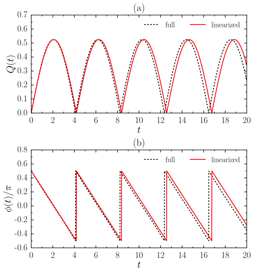
Figure 7: Predictions of the bimetric theory for (a) $Q$ and (b) $\phi$ under the initial condition $Q(0)=0$. Black dashed lines indicate the numerical solution of the full equations, Eqs. (19) and (20). Red solid lines indicate the analytical solution (7) and (8) of the linearized system, Eqs. (24) and (25). Here, we focus on the $Q\geq 0$ solution. The parameters are fixed at $\Omega=1.5/4$, $\gamma=-1$, $A=\ln 1.3$.

V.5 Agreement between bimetric theory and exact dynamics

Since Eqs. (24)-(25) are an accurate approximation of Eqs. (19)-(20) in the adiabatic quench regime, we were justified in fitting our exact results in Sec. IV against simple harmonic oscillation in Eqs. (7)-(8). The fits allow us to extract the values of $A$ and $E_{\gamma}$, which we can now interpret as the intrinsic anisotropy and graviton gap in the bimetric theory.

By extracting $E_{\gamma}$ from the fitting of quench data for various initial parameters, we indeed find that the obtained $E_{\gamma}$ is insensitive to the precise values of $A_{0}$ and $A_{1}$, as long as we are in the adiabatic quench regime. On the other hand, $A$ quantifies the intrinsic anisotropy in the ground state of $H^{\prime}$, which is a compromise between $g_{m}^{\prime}$ and $g_{i}^{\prime}$. Since we do the same modification for $g_{m}$ and $g_{i}$ in the quench driven by the contact interaction, we expect $A=A_{1}$ in this case. Indeed, we get $A\approx 0.255$ from the fit in Fig. 3, which is very close to $A_{1}=\ln 1.3\approx 0.262$. However, in the quench driven by the Coulomb interaction, we keep isotropic $g_{i}$ and only change $g_{m}$, so the intrinsic anisotropy in the ground state of $H^{\prime}$ is expected to be weaker than $g_{m}^{\prime}$. The fit in Fig. 4 gives $A\approx 0.454$, which is indeed between $0$ and $A_{1}=\ln 2.0\approx 0.693$.

In summary, we find that adiabatic isotropic-anisotropic mass anisotropy quenches in the Laughlin phase can be described as harmonic motion of a single spin-$2$ degree of freedom, in agreement with the bimetric theory. Minor deviations from harmonic motion can be observed in Figs. 3 and 4 at longer times. These deviations generally have two manifestations: as a decay in amplitude while maintaining the overall oscillation structure, or as a total departure from the oscillation. The former is mainly the case for isotropic-to-anisotropic quenches considered in Figs. 3 and 4, while the latter can be observed in the more general case of anisotropic-to-anisotropic quench considered in Appendix A as well as in some fermionic data in Appendix D.

There are several possible explanations for the discrepancy with the bimetric theory. First, in finite systems a “fragmentation” of the spin-$2$ graviton mode into several states with large matrix element $|\langle n|\hat{V}_{0,2}|0\rangle|^{2}$ (as seen in Fig. 5) induces several close frequencies in the dynamics. With the available data for system sizes up to $N=12$, there is no clear indication that this fragmentation disappears in the thermodynamic limit, even though a “sharp” spin-$2$ mode is theoretically anticipated in large systems. This suggests that finite size effects, to the zeroth order, do not seem to be the explanation for the fragmentation. Note that the fragmentation for the Coulomb interaction is much weaker than that for the contact interaction (Fig. 5), reflecting a more isolated graviton mode in the Coulomb case. A more likely source of “finite-time” errors in the dynamics could be due to an effective Lieb-Robinson Lieb and Robinson (1972) “light cone” exceeding the finite size of the system. Finally, the discrepancy could arise due to the contribution of higher-spin modes to the dynamics. In the following section, we design more complex type of quenches to probe such modes. These quenches lead to non-trivial dynamics which is not accounted for in the bimetric theory or its direct extensions in Eqs. (7)-(8).

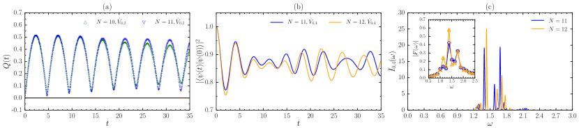
Figure 8: (a) Exact dynamics of $Q$ for the quench with $\hat{V}_{0}\rightarrow\hat{V}_{0}+0.1\hat{V}_{0,2}$ (color symbol) and $\hat{V}_{0}\rightarrow\hat{V}_{0}+0.1\hat{V}_{0,4}$ (black solid line). A complete absence of dynamics of $\hat{g}$ can be noticed in the case of the perturbation by $\hat{V}_{0,4}$. (b) Dynamics of quantum fidelity, $|\langle\psi(t)|\psi(0)\rangle|^{2}$, for the quench with $\hat{V}_{0}\rightarrow\hat{V}_{0}+0.1\hat{V}_{0,4}$. (c) Normalized spectral function ${\bar{I}}_{0,4}(\omega)=I_{0,4}(\omega)/\int I_{0,4}(\omega)d\omega$ for isotropic systems of $N=11$ and $12$ bosons at $\nu=1/2$ with contact interaction. The inset shows the discrete Fourier transform $|F(\omega)|$ of $|\langle\psi(t)|\psi(0)\rangle|^{2}$. Markers in insets and curves in main figures with the same color refer to the same system size.

VI Higher-spin modes

VI.1 $W_{\infty}$ algebra in the lowest Landau level

It has been realized a long time ago that the lowest Landau level admits an action of the (infinite-dimentional) algebra of area-preserving diffeomorphisms (APD), $W_{\infty}$ Girvin et al. (1986); Cappelli et al. (1993). The action of this algebra can be interpreted as area-preserving distortions of FQH droplets, illustrated in Fig. 1. These distortions, however, cost finite energy since the interaction potential, Eq. (1), is not invariant under these transformations Girvin et al. (1986); Haldane (2011). Consequently, the gapped spin-$2$ mode discussed in the previous section can be viewed as a particular, quadrupolar, APD of the droplet. This fact is reflected in the bimetric theory, in the form of hidden $sl(2,\mathbb{R})$ (which is the largest finite-dimensional subalgebra of $W_{\infty}$) symmetry Gromov and Son (2017). The topological part of the action in Eq. (10) is invariant under the action of $sl(2,\mathbb{R})$, while the Hamiltonian explicitly breaks it down to $so(2)\subset sl(2,\mathbb{R})$. Thus the application of the (broken) shear generators of $sl(2,\mathbb{R})$, represented by the off-diagonal components of the emergent metric $\hat{g}_{ij}$, leads to the creation of an excited spin-$2$ state.

Naturally, one may expect that higher angular momentum distortion of the fluid will correspond to independent collective modes, at least at long wavelengths Cappelli and Randellini (2016); Golkar et al. (2016b). The construction of an effective theory describing the infinite number of interacting higher spin fields is not an easy task, and has been an outstanding problem for a long time. A significant advance in solving this problem in $(2+1)D$ was made in Blencowe (1989); Bergshoeff et al. (1990), where Chern-Simons-type action for higher spin gravity was constructed. Presently, it is not understood how these ideas can be applied to the FQH problem.

The algebra of APDs made multiple appearances in the FQH problem: non-commutative Chern-Simons theory Susskind (2001), matrix models Polychronakos (2001); Hellerman and Raamsdonk (2001), bosonization of the LLL problem Iso et al. (1992), manifestly LLL-projected description of the CFL-type state of bosons at $\nu=1$ Read (1998). Higher-spin degrees of freedom naturally appear in the composite fermion approach to the Jain series at filling $\nu=\frac{n}{2n+1}$, at large values of $n$ (i.e., close to half-filling) Golkar et al. (2016b); Nguyen et al. . Those theories describe free massive higher spin fields with a quadratic action. Consequently, the (inherently non-linear) $W_{\infty}$ structure is invisible. In what follows we provide evidence, obtained directly from the microscopic quench dynamics, that at long distances the electrons forming an FQH fluid support collective modes of higher spin. The evidence is obtained by designing a quench protocol that selectively excites the higher-spin collective modes.

VI.2 Higher-spin quench

Tuning the anisotropy of the mass tensor is an experimentally relevant mechanism for changing the metric in the interaction. However, this also leads to the modification of the entire set of coefficients $c_{m,n}$ of the generalized Haldane pseudopotentials $\hat{V}_{m,n}$ [Eq. (5)], which uniquely characterize the interaction:

$$\bar{V}_{\mathbf{q}}=\sum_{m,n}c_{m,n}V_{m,n}(\mathbf{q}).$$ (26)

Modifying individual coefficients $c_{m,n}$, one at a time, is a much more controlled way to drive a quench. While this may not be easily achievable in experiment, this new quench protocol allows for more control in probing different types of dynamics. As we show below, reformulating the quench protocol in this way not only includes the former scenario of changing the mass tensor, but also reveals new types of dynamics, which lie beyond the single mode approximation and the bimetric theory.

To perform the quench, we prepare a state annihilated by the Hamiltonian with $c_{m,n}=\delta_{n,0}\delta_{m,0}$. Then, a nonzero $c_{0,2}=0.1$ is introduced at $t=0^{+}$. This corresponds to the modification of the interaction $\hat{V}_{0}\to\hat{V}_{0}+0.1\hat{V}_{0,2}$. Since $\hat{V}_{0,2}$ carries angular momentum $L_{z}=2$, we expect that its presence will drive a quench dominated by the spin-$2$ mode. Indeed, we find that the consequent exact dynamics of $\hat{g}$ behaves according to the description based on the spin-$2$ graviton oscillation [Fig. 8(a)], and is very similar to that obtained by changing the mass tensor in Fig. 3.

Next, we consider a quench driven by adding a small amount of $\hat{V}_{0,4}$ component ($c_{0,4}=0.1$) such that the interaction changes according to $\hat{V}_{0}\to\hat{V}_{0}+0.1\hat{V}_{0,4}$ at $t=0^{+}$. This type of quench can be realized in systems whose Fermi contours are not simple ellipses, e.g., where the band dispersion has the form $\epsilon(\mathbf{k})=k^{N}\cos(N\theta)$ Haldane and Shen ; Ippoliti et al. (2017). As shown in Ref. Ippoliti et al. (2017), when $N=4$, the dominant anisotropic pseudopotential is $V_{0,4}$. Surprisingly, we find $Q(t)\equiv 0$ during the entire measured time interval [see the black solid line in Fig. 8(a)], which suggests that the spin-$2$ collective mode is not excited. However, the system does respond to the perturbation by $\hat{V}_{0,4}$, and we conjecture that this happens by exciting the higher-spin collective modes, which cannot be described by the bimetric theory. While we cannot describe the dynamics of higher-spin modes analytically, we can measure the dynamics of quantum fidelity, $|\langle\psi(t)|\psi(0)\rangle|^{2}$, shown in Fig. 8(b). Clear oscillations in the fidelity are a signature of the non-trivial microscopic dynamics taking place. We note that in the case of $\hat{V}_{0,2}$ quench, fidelity also oscillates, with the same frequency as $\hat{g}$. Moreover, we emphasize that our choice of measuring fidelity was merely a convenience; indeed, observables like entanglement entropy also display quantitatively similar oscillations.

The failure of the bimetric theory to capture the quench dynamics driven by $\hat{V}_{0,4}$ strongly suggests that the $\hat{V}_{0,4}$ quench is dominated by a higher-spin collective mode rather than the spin-$2$ one. Indeed, unlike the quadrupolar $\hat{V}_{0,2}$, $\hat{V}_{0,4}$ has octupolar structure in momentum space [Fig. 2(b)], which implies that it would couple the ground state to higher-spin excitations. In our case, this is a spin-4 excitation because the odd-spin ones vanish due to inversion symmetry, which is a generic symmetry of LLL-projected FQH Hamiltonians. The spin-4 character of the mode is explicitly confirmed by evaluating the spectral function $\bar{I}_{0,4}(\omega)$ in Fig. 8(c) (with identical results obtained for the discrete Fourier transform, shown in the inset of the same figure). The spectral function shows two peaks, one of which corresponds to the graviton energy and an additional one at higher energy, $\omega\sim 1.7$, which we identify with spin-4 mode. This provides an unambiguous example in which the $2\times 2$ unimodular metric in Eq. (4) is inadequate to capture the dynamics of the Laughlin state, motivating the generalization of the geometrical description of the fractional quantum Hall states and the effective field theory.

VII Conclusions and outlook

In the present manuscript we have laid out the theoretical foundation for studying the nonequilibrium dynamics of FQH states. We have proposed and numerically simulated the geometric quench protocol that excites neutral collective degrees of freedom of FQH liquids, such as the Laughlin states of bosons at $\nu=1/2$ and of fermions at $\nu=1/3$. In all the cases, for the simplest types of quenches, which are driven by modifying the mass tensor, we have established that the short-time dynamics after the quench is dominated by the spin-$2$ graviton mode and accurately agrees with the bimetric theory. Furthermore, we have demonstrated that the geometric quench protocol admits a generalization that allows one to excite higher-spin collective degrees of freedom, whose dynamics cannot be described by the currently available geometric theories of the FQH effect. We believe that the present work will motivate a more detailed study of the geometric degrees of freedom in various strongly correlated systems, and below we highlight several directions that open up for future investigations.

The immediate question that arises is the experimental applicability of our results. Even though the quench protocol can in principle be directly implemented with the available technology, the main challenge is observing coherent dynamics in solid-state materials that currently support FQH states. Assuming typical magnetic fields $10$T, we estimate the required time scales for observing the graviton oscillation to be $\sim 10^{-14}$s, which is prohibitively small. The second challenge is how to measure the intrinsic metric in gapped FQH states. Recent experiments have successfully measured the anisotropy of the composite fermion Fermi surface induced by tilting the magnetic field Kamburov et al. (2013, 2014). Similar measurements were also performed for hole systems Mueed et al. (2015). However, such experiments still need to be generalized to gapped FQH states (we note that acoustic wave absorption has been theoretically proposed as an alternative spectroscopic probe of the graviton Yang (2016)). Given the smallness of time scales in solid state FQH materials, a more versatile platform to observe geometric quench could be their analogs in lattice systems – the fractional Chern insulators (FCIs) Parameswaran et al. (2013); Bergholtz and Liu (2013); Neupert et al. (2015); Spanton et al. (2018). As we demonstrate in Appendix E, a geometric quench that excites a spin-2 mode can be straightforwardly implemented in an FCI, resulting in the same type of dynamics described by the bimetric theory in the long-wavelength limit. The tunability of parameters in FCIs allows one to observe time scales on the order of $\sim 10^{-5}$s (assuming the interaction strength in cold-atom settings is in the order of $2\pi\hbar\times 10$kHz), which is well within the limits of recent experiments Bernien et al. (2017).

New dynamical phenomena will likely arise in Abelian FQH states with more complicated internal structure, such as bi-layer states and Jain states. These states host multiple collective modes which would all contribute to the dynamics. Multi-layer systems feature rich phase diagrams that can be explored by tuning the interaction strength between the layers Gir (2007); Eisenstein (2014). It would be interesting to map out the dynamical counterparts of such equilibrium phase diagrams by studying the geometric quench in different interaction regimes.

Even in the simplest models of Laughlin states, our study has focused on the linear regime of adiabatic quench. The non-linear regime should become relevant for strong quenches or quenches in the vicinity of the nematic phase transition. The present quench protocol could be used as a complementary tool for probing the nematic transition, which has recently been studied in Ref. Regnault et al. (2017).

When a “higher-spin” pseudopotential drives the quench, the system undergoes non-trivial dynamics which cannot be described within the bimetric theory or by anisotropic trial states Qiu et al. (2012). In these cases, a richer set of trial states is needed to fully describe the dynamics. This set of states should be parametrized by higher-spin cousins of the intrinsic metric $\hat{g}$. Similar conclusions were reached in Ref. Gromov and Son (2017) (see also Ref. Cappelli and Randellini (2016)) where the bimetric theory was argued to be a low-energy approximation to a putative higher-spin theory, and in Ref. Nguyen et al. where the linearized bimetric for the Jain series at $\nu=n/(2n+1)$ was derived from the Dirac composite Fermi liquid (CFL) theory at large $n$. In the latter approach the higher-spin modes naturally emerge as collective distortions of the composite Fermi surface. In fact, when the CFL state forms, all of the higher-spin degrees of freedom become gapless, and should be equally important for the dynamics. In these systems, the geometric quench described in the present manuscript, as well as its “higher-spin” cousins, will provide an interesting probe of the collective dynamics of the composite fermion Fermi surface.

The geometric quench also presents an enticing possibility of probing the non-Abelian fractional quantum Hall states, such as the Moore-Read state Moore and Read (1991) – a candidate for the observed $\nu=5/2$ plateau Willett et al. (1987). Numerical works Bonderson et al. (2011); Möller et al. (2011) have shown that the Moore-Read state hosts a neutral fermionic mode, in addition to the SMA (bosonic) mode. The neutral fermion mode is expected to have angular momentum $3/2$ and is not present in the bimetric theory. It would be very interesting to design the effective theory and numerical probes of this mode at long wavelengths.

Finally, FCIs exhibit much of the same phenomenology as the continuum FQH states (see the recent reviews Refs. Parameswaran et al. (2013); Bergholtz and Liu (2013); Neupert et al. (2015) and references therein). For example, the FCIs also feature the GMP algebra Scaffidi and Simon (2014); Roy (2014), and they naturally correspond to anisotropic FQH states Harper et al. (2014); Yang et al. (2017a). On the other hand, the FCI states in higher Chern number bands Liu et al. (2012); Wang et al. (2012b); Sterdyniak et al. (2013) do not have the usual continuum FQH states as their counterparts Wu et al. (2013). Given that the quench driven by anisotropy in hopping has been studied for integer Chern insulators Killi and Paramekanti (2012); Killi et al. (2012), it would be interesting to investigate more systematically the quenches for FCIs, starting from the basic method that we have presented in Appendix E.

Appendix A Anisotropic-to-anisotropic quench

As an immediate generalization of the isotropic-to-anisotropic quench studied in Sec. IV.1, we now discuss the more general case of a quench with $A_{1}>A_{0}>0$, for which the initial state is already anisotropic. In this case, a simple analytical solution does not exist under the general initial conditions $Q(0)>0,\phi(0)=0$ even for the linearized systems (24) and (25). However, by numerically solving the coupled differential equations, we find that the bimetric theory still accurately describes the short-time dynamics of $Q$ and $\phi$, and also captures the oscillatory dynamics very well up to moderate times.

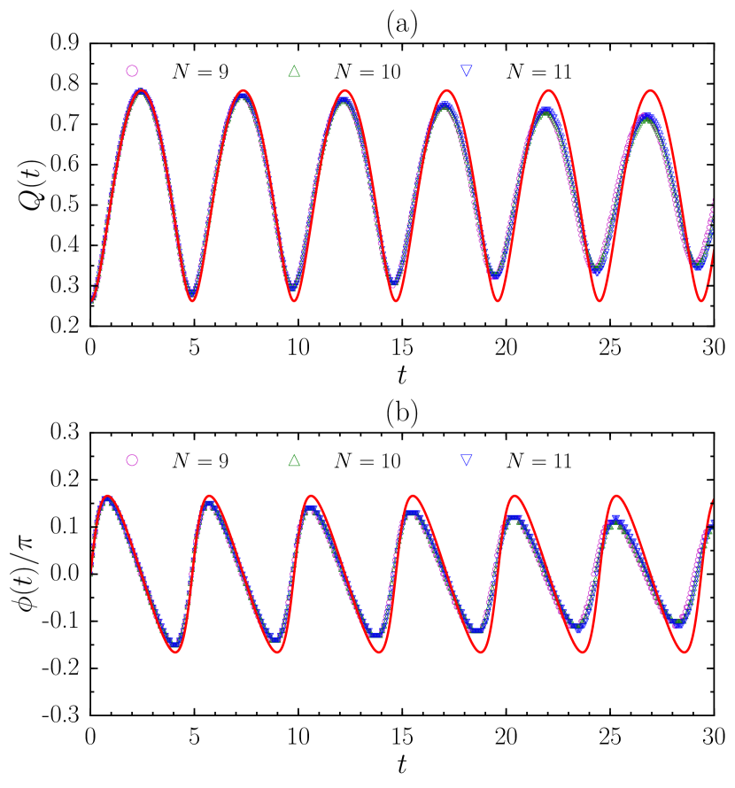
Figure 9: Exact dynamics of (a) $Q$ and (b) $\phi$ for $N=9-11$ bosons at $\nu=1/2$ with the contact interaction. The adiabatic geometric quench is driven by choosing $A_{0}=\ln 1.3$ and $A_{1}=\ln 1.7$. The red solid curve is the solution of linearized equations (24) and (25) under the initial condition $Q(0)=A_{0},\phi(0)=0$, with $A\approx 0.523$ and $E_{\gamma}\approx 1.283$. These two parameters are obtained by fitting the first oscillation of $Q$ of $N=11$ against the solution.

In Fig. 9, we choose $A_{0}=\ln 1.3$ and $A_{1}=\ln 1.7$, and show the exact dynamics for the quench driven by the contact interaction. Since the initial state is a Laughlin model state with $\hat{g}(0)=g_{m}$, the bimetric theory predicts the post-quench dynamics of $\hat{g}$ is governed by the solution of Eqs. (24) and (25) with initial condition $Q(0)=A_{0},\phi(0)=0$. Indeed, the numerical data in the first two periods again lie on top of such a solution with fitting parameters $A\approx 0.523$ and $E_{\gamma}\approx 1.283$. The value of $A$ is close to $A_{1}=\ln 1.7\approx 0.531$, as expected, and $E_{\gamma}\approx 1.283$ is consistent with the graviton gap estimated from both the $I_{0,2}(\omega)$ spectral function and the previous fit in Fig. 3.

As discussed in Sec. IV.1, apart from generally good agreement, we can also observe some discrepancy between the exact dynamics and the equations of the bimetric theory in Fig. 9. This discrepancy is likely caused by the mentioned finite-size effect (the splitting of the spin-$2$ mode into several states and the Lieb-Robinson light cone) and the possible contribution of higher-spin modes. Compared to isotropic-to-anisotropic quench, stronger finite-size effects in the present case are not surprising because anisotropy effectively reduces the length of the system along one of the spatial directions.

Appendix B Projected dynamics

In the main text, we have shown that the number of spin-$2$ eigenstates of $H^{\prime}$ is exponentially smaller than the full Hilbert space dimension. The number of spin-2 eigenstates was determined by the matrix element of $\hat{V}_{0,2}$ generalized pseudopotential. Here we investigate how accurately the quench dynamics in Sec. IV.1 can be reproduced by projecting to this set of states.

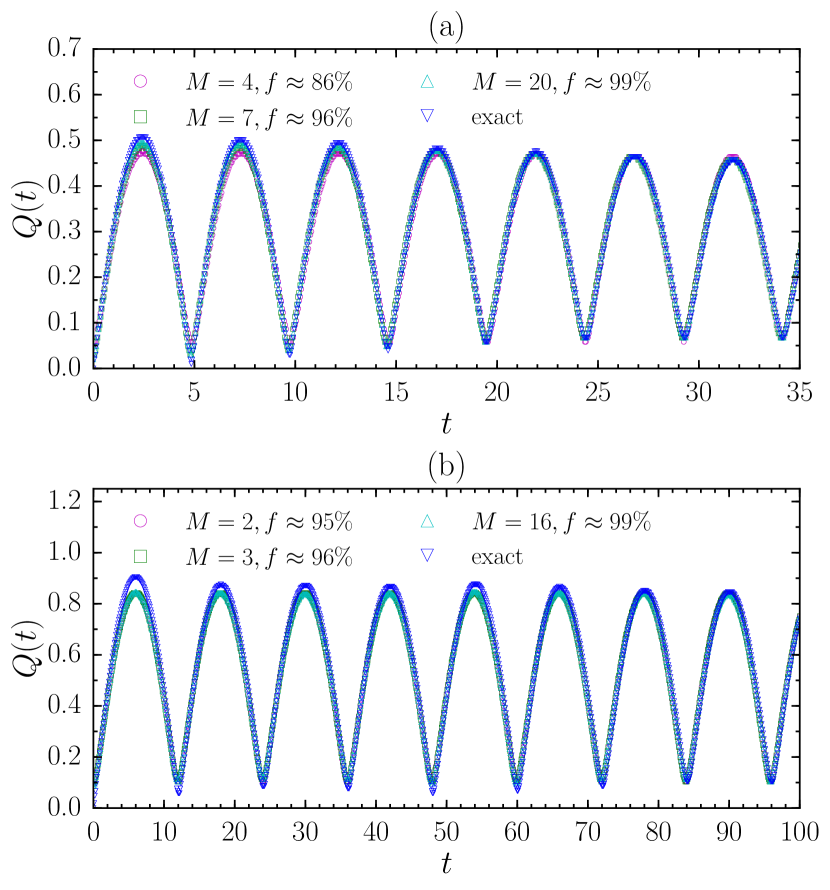
Figure 10: Dynamics of $Q$ projected to $M$ eigenstates of $H^{\prime}$ with dominant $|\langle n|\hat{V}_{0,2}|0\rangle|^{2}$. We consider $N=11$ bosons at $\nu=1/2$ with (a) contact and (b) Coulomb interactions. The quench parameters $A_{0}$ and $A_{1}$ are the same as those in Figs. 3 and 4, respectively.

We perform the projection explicitly, i.e., we calculate the post-quench state as $|\tilde{\psi}(t)\rangle=\frac{1}{\mathcal{N}}\sum_{n\in\mathcal{S}}\exp(-i\epsilon_{n}t)\langle n|\psi_{0}\rangle|n\rangle$, where $\mathcal{S}$ contains the first $M$ eigenstates with the largest $|\langle n|\hat{V}_{0,2}|0\rangle|^{2}$ matrix elements and $\mathcal{N}$ is the normalization factor. The dynamics of the intrinsic metric of $|\tilde{\psi}(t)\rangle$ after an isotropic-anisotropic quench is shown in Fig. 10 for $N=11$ bosons, together with exact dynamics without the projection. As expected, the projected dynamics approaches the exact dynamics with increasing $M$. However, for both contact and Coulomb interactions, the main feature in exact dynamics has been accurately reproduced by $M$ less than $10$, even if the whole Hilbert space in this case is more than four orders of magnitude larger. Such an excellent approximation of the exact dynamics by a tiny spin-$2$ fraction of the whole Hilbert space is an evidence for the picture of graviton oscillation and the bimetric theory.

Appendix C Non-instantaneous quench

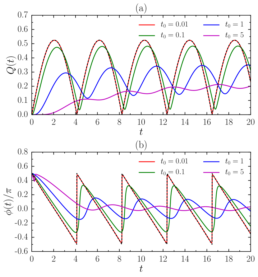
Figure 11: Solutions of the full equations [Eqs. (19) and (20)] for the non-instantaneous quench with $A(t)=A_{1}\exp{(-t_{0}/t)}$, under the initial condition $Q(0)=0$. Here we focus on the $Q\geq 0$ solution. We choose $\Omega=1.5/4,\gamma=-1,A_{1}=\ln 1.3$, and consider several different $t_{0}=0.01$, $0.1$, $1$ and $5$. For comparison, we also give solutions for the instantaneous quench as black dashed lines.

Instantaneous quench is the minimal theoretical model that describes sudden tilt of the magnetic field. However, since any experimental manipulation takes finite time, we now generalize our discussions to more realistic, non-instantaneous quenches. To be specific, we consider isotropic-anisotropic quenches driven by a time-dependent ramp of the mass tensor, i.e., $g_{m}={\rm diag}(e^{A(t)},e^{-A(t)})$ with

$$A(t)=A_{1}\exp(-t_{0}/t),$$ (27)

such that $A(0)=0$ and $A(+\infty)=A_{1}$. The slope of the ramp depends on some characteristic time, $t_{0}$. When $t_{0}=0$, we recover the instantaneous quench studied in Sec. IV.1. We thus expect that differences between the non-instantaneous quench and the instantaneous one are negligible when $t_{0}$ is small, while some qualitative changes may happen for large enough $t_{0}$.

As a representative example, we choose $A_{1}=\ln 1.3$ (adiabatic quench) and show the predicted behavior of $Q$ and $\phi$ in the bimetric theory, i.e., the solutions of the full equations [Eqs. (19) and (20)], for different $t_{0}$ in Fig. 11. We indeed find that the solutions in the non-instantaneous case agree with their instantaneous limit up to $t_{0}\lesssim 10^{-2}$. The effect of the ramp starts to appear when $t_{0}\sim 10^{-1}$, which leads to gradual deviations of both the amplitude and frequency in the dynamics from the instantaneous case. Finally, for very large $t_{0}\gtrsim 1$, we observe strongly distorted oscillation patterns in $Q$ and $\phi$, revealing very different dynamics between the fast-quench and slow-quench regimes.

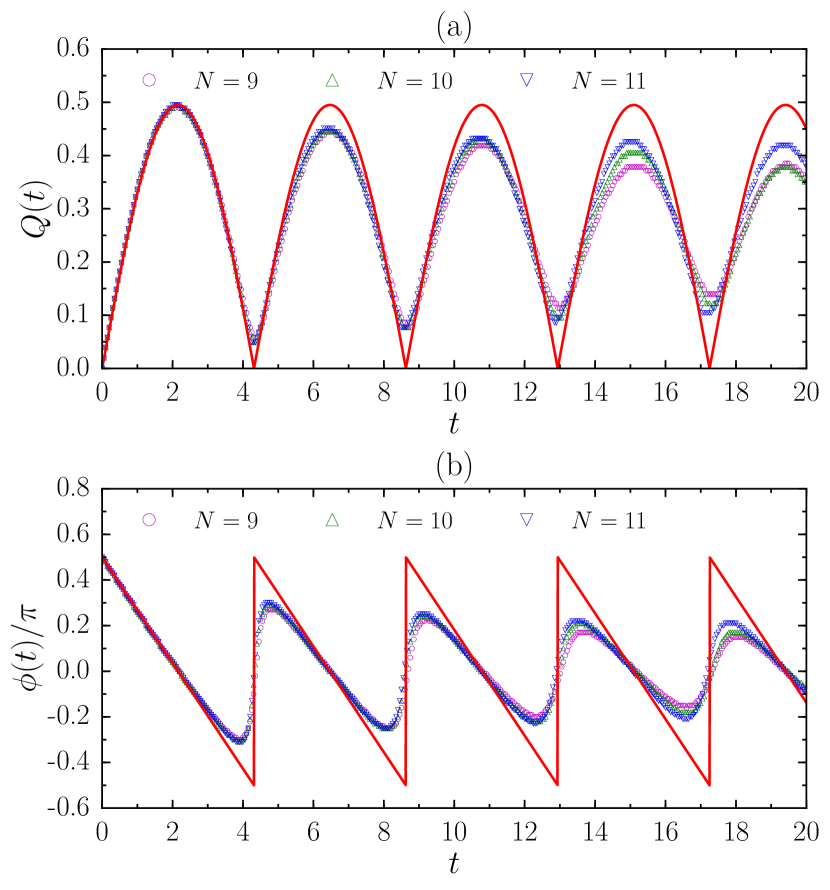
Figure 12: Exact dynamics of (a) $Q$ and (b) $\phi$ for $N=9-11$ fermions at $\nu=1/3$ with the $V_{1}$ interaction. The adiabatic geometric quench is driven by choosing $A_{0}=0$ and $A_{1}=\ln 1.3$. The red solid curve is the $Q\geq 0$ part of Eqs. (7) and (8), with $A\approx 0.248$ and $E_{\gamma}\approx 1.457$. These two parameters are obtained by fitting the first oscillation of $Q$ of $N=11$ against the solution.

It would be interesting to compare the exact dynamics of finite systems with the predictions of the bimetric theory also for non-instantaneous quenches, as we have done for the instantaneous case in Sec. IV. Due to the time-dependent nature of the non-instantaneous quench, the many-body numerical simulation in this case is more complicated and will be presented in future work. However, because the instantaneous quench corresponds to a stronger perturbation of the system, we expect similar or better agreement between theory and numerics for the case of non-instantaneous quenches.

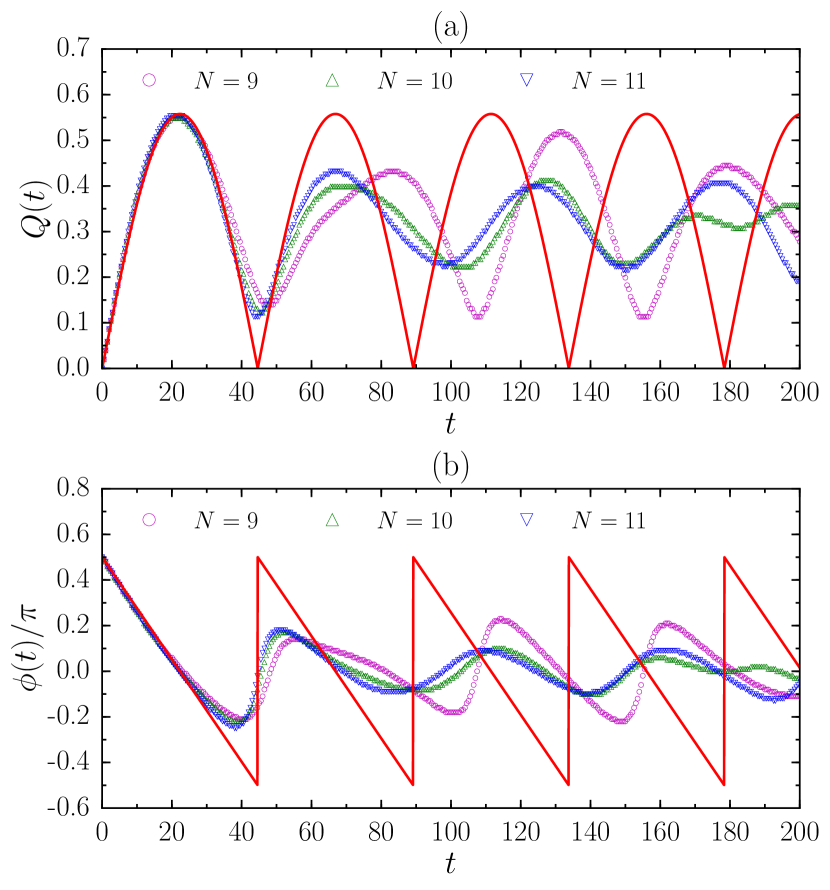
Figure 13: Exact dynamics of (a) $Q$ and (b) $\phi$ for $N=9-11$ fermions at $\nu=1/3$ with the Coulomb interaction. The adiabatic geometric quench is driven by choosing $A_{0}=0$ and $A_{1}=\ln 2.0$. The red solid curve is the $Q\geq 0$ part of Eqs. (7) and (8), with $A\approx 0.279$ and $E_{\gamma}\approx 0.141$. These two parameters are obtained by fitting the first oscillation of $Q$ of $N=11$ against the solution.

Appendix D Adiabatic geometric quench for $\nu=1/3$ fermions

Here we show the numerical results of the exact dynamics of $\hat{g}$ after a mass anisotropy quench for $\nu=1/3$ fermions. As representative examples, we focus on adiabatic isotropic-anisotropic quenches with $A_{0}=0$ and $A_{1}>0$, where we choose $A_{1}=\ln 1.3$ and $A_{1}=\ln 2.0$ for quenches driven by $V_{1}$ and Coulomb interactions, respectively. Exact dynamics of $\hat{g}$ up to moderate times is shown in Figs. 12 and 13 for these two types of interactions.

Similar to $\nu=1/2$ bosons, the short-time dynamics of adiabatic quenches for $\nu=1/3$ fermions fully agrees with the bimetric theory. We can thus extract parameters $A$ and $E_{\gamma}$ by fitting the numerical data against Eqs. (7) and (8), whose values are given in the captions of Figs. 12 and 13. The value of $A$, which quantifies the anisotropy in the interaction, is again close to $A_{1}$ (between $0$ and $A_{1}$) for the $V_{1}$ (Coulomb) interaction as expected. The value of $E_{\gamma}$ estimates the graviton gap as $1.46$ and $0.14$ for $V_{1}$ and Coulomb interactions, respectively. Note that the graviton gap of the Coulomb interaction that we extract from the quench dynamics precisely matches the value given by other methods in the context of single-mode approximation Girvin et al. (1985, 1986).

Like in the bosonic case, we also observe deviations from the bimetric theory at longer times for $\nu=1/3$ fermions. However, these deviations are more serious and appear earlier than those for $\nu=1/2$ bosons. For quenches driven by the $V_{1}$ interaction, while the overall oscillation structure is maintained up to moderate times, the oscillating amplitude already visibly decays after the first oscillation (Fig. 12). The situation is even worse for quenches driven by the Coulomb interaction, as expected. In that case, the behavior of $Q$ and $\phi$ totally departs from simple oscillations after the first period and the curves of different system sizes are no longer on top of each other (Fig. 13). Compared with $\nu=1/2$ bosons, our numerical results clearly demonstrate that the dynamics of $\nu=1/3$ fermions suffers more from finite-size effects in the excitations and the participation of higher-spin modes.

Appendix E Fractional Chern insulators

Here we generalize the geometric quench from continuum FQH states to their lattice analogs – the fractional Chern insulators (FCIs) Parameswaran et al. (2013); Bergholtz and Liu (2013); Neupert et al. (2015). Contrary to conventional FQH states, FCIs do not require an external magnetic field Sun et al. (2011); Neupert et al. (2011) and may potentially persist at higher temperatures Tang et al. (2011). Considering the recent experimental progress on quantum many-body dynamics in optical lattices Langen et al. (2015), FCIs realized by cold atoms in optical lattices could be a promising platform to observe the dynamics after a geometric quench on much longer time scales than possible in semiconductor FQH systems. In the following, we will describe a quench protocol for FCIs and demonstrate that our main results directly apply to this type of system. As FCIs are inherently anisotropic, the quenches in FCI belong to the anisotropic-anisotropic case discussed in Appendix A.

For concreteness, we consider $N$ bosons in a two-dimensional Ruby lattice Hu et al. (2011) of $N_{1}\times N_{2}$ unit cells. The system is in $xy$ plane with periodic boundary conditions. We adopt the same tight-binding parameters and lattice configurations as in Ref. Wu et al. (2012), for which the lowest Bloch band is flat and has Chern number $C=1$. We assume that bosons interact via onsite and dipolar potentials. If all dipoles are polarized in $xz$ plane with an angle $\alpha$ to the $+z$ direction, the interaction Hamiltonian can be written as

$$H_{\rm int}=\sum_{i}n_{i}(n_{i}-1)+\sum_{i<j}\frac{r_{ij}^{2}-3x_{ij}^{2}\sin^{2}\alpha}{r_{ij}^{5}}n_{i}n_{j},$$

(28)

where $n_{i}$ is the occupation on lattice site $i$, and $r_{ij}=(x_{ij},y_{ij})$ is the distance between lattice site $i$ and $j$. We project the interaction to the lowest band and verify that the ground state at band filling $\nu=N/(N_{1}N_{2})=1/2$ is the $\nu=1/2$ bosonic Laughlin FCI for a finite range of $\alpha$, characterized by a robust two-fold topological degeneracy. In order to keep the lattice aspect ratio close to $1$ and for the two degenerate FCI states to be located in different momentum sectors, we focus on two system sizes below: $N=6,N_{1}=3,N_{2}=4$ and $N=10,N_{1}=4,N_{2}=5$.

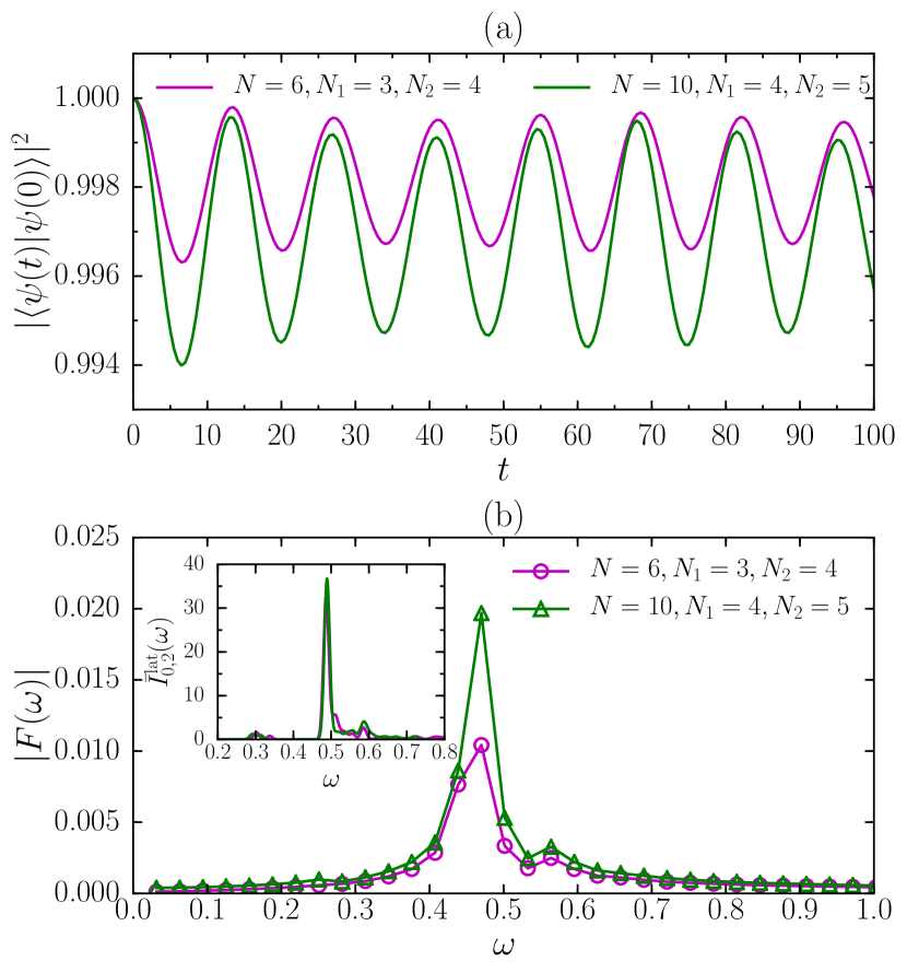
Figure 14: (a) Dynamics of fidelity, $|\langle\psi(t)|\psi(0)\rangle|^{2}$, and (b) its discrete Fourier transform for $\nu=1/2$ bosonic Laughlin FCIs. The adiabatic quench is driven by $\alpha^{\prime}=15^{\circ}$. The inset of (b) shows the normalized spectral function ${\bar{I}}_{0,2}^{\rm lat}(\omega)=I_{0,2}^{\rm lat}(\omega)/\int I_{0,2}^{\rm lat}(\omega)d\omega$ for the isotropic case with $\alpha=0$. Markers in insets and curves in main figures with the same color refer to the same system size.

While the interaction is isotropic for $\alpha=0$, tuning $\alpha$ away from $0$ adds anisotropy, which can be experimentally achieved by changing the direction of the polarizing magnetic field Baier et al. (2016). We prepare the initial state as the ground state with momentum ${\bf K}={\bf 0}$, then drive the quench by suddenly changing $\alpha$ from $0$ to a small but finite $\alpha^{\prime}$ (adiabatic quench). Tuning $\alpha$ is not a direct lattice analog of changing the geometry of continuum Landau level orbitals, but it is also expected to excite a geometric degree of freedom in FCIs because it adds quadrupolar anistropy in the system. In order to confirm this, we track the dynamics of fidelity $|\langle\psi(t)|\psi(0)\rangle|^{2}$, and compare its dominant frequency with the energy of FCI graviton mode which can be probed by a suitable lattice analog of the $\hat{V}_{0,2}$ pseudopotential. A detailed study of intrinsic metric is also feasible for FCIs by the FCI-FQH mapping Wu et al. (2013) and will be presented in a future work.

In Fig. 14, we show the fidelity and its discrete Fourier transform for $\alpha^{\prime}=15^{\circ}$. One can see that the dynamics of fidelity is dominated by a single frequency, characterized by the pronounced peak at $\omega\approx 0.47$ in the discrete Fourier transform [Fig. 14(b)]. In order to estimate the graviton energy on the lattice, we define the operator

$$\hat{V}_{0,2}^{\rm lat}=\sum_{{\bf q}}(\cos q_{1}-\cos q_{2}){\bar{\rho}_{\bf q}}^{\rm lat}\bar{\rho}_{-{\bf q}}^{\rm lat},$$ (29)

where $q_{i}={\bf q}\cdot{\bf b}_{i}$ with ${\bf b}_{i}$’s the two basic lattice direction vectors, ${\bf q}$ is in the first Brillouin zone, and $\bar{\rho}_{\bf q}^{\rm lat}$ is the density operator $e^{i{\bf q}\cdot\hat{{\bf r}}}$ projected to the lowest Bloch band (see Refs. Parameswaran et al. (2012); Bernevig and Regnault (2012); Wu et al. (2013); Repellin et al. (2014) for the explicit form of $\bar{\rho}_{\bf q}^{\rm lat}$). Similar to the continuum $\hat{V}_{0,2}$ pseudopotential, $\hat{V}_{0,2}^{\rm lat}$ effectively carries angular momentum $L_{z}=2$ to probe spin-$2$ states on the lattice, because the ${\bf q}$-dependent term $\cos q_{1}-\cos q_{2}$ takes a $d$-wave form $q_{1}^{2}-q_{2}^{2}$ at small $|{\bf q}|$. Indeed, its spectral function

$$I_{0,2}^{\rm lat}(\omega)=\sum_{j}\delta(\omega-\epsilon_{j})|\langle j|\hat{V}_{0,2}^{\rm lat}|0\rangle|^{2}$$ (30)

shows sharply pronounced peaks [inset of Fig. 14(b)], where $\epsilon_{j}$ and $|j\rangle$ are the eigen-energy and eigenstate of the projected interaction (28). Since these peaks appear around the same energy as that in the discrete Fourier transform of fidelity, our quench protocol indeed excites the geometric degree of freedom of FCI that corresponds to the spin-$2$ graviton mode on a lattice. The similarity of the FCI results to the continuum FQH is rather surprising, in light of the fact that there are no quantitative arguments that support the relation between the bimetric theory and FCIs (beyond the intuition mentioned in Ref. Gromov and Son (2017)).

References

- Laughlin (1983) R. B. Laughlin, Phys. Rev. Lett. 50, 1395 (1983).
- Wen (1990) X. G. Wen, Int. J. Mod. Phys. B 04, 239 (1990).
- Halperin (1982) B. I. Halperin, Phys. Rev. B 25, 2185 (1982).
- Wen (1991) X. Wen, Modern Physics Letters B 05, 39 (1991).
- Prange and Girvin (1987) R. E. Prange and S. M. Girvin, The Quantum Hall effect (Springer-Verlag, 1987).
- Tsui et al. (1982) D. C. Tsui, H. L. Stormer, and A. C. Gossard, Phys. Rev. Lett. 48, 1559 (1982).
- Jain (1989) J. K. Jain, Phys. Rev. Lett. 63, 199 (1989).
- Moore and Read (1991) G. Moore and N. Read, Nuclear Physics B 360, 362 (1991).
- Read and Rezayi (1999) N. Read and E. Rezayi, Phys. Rev. B 59, 8084 (1999).
- Zhang et al. (1989) S. C. Zhang, T. H. Hansson, and S. Kivelson, Phys. Rev. Lett. 62, 82 (1989).
- Wen and Zee (1992a) X. G. Wen and A. Zee, Phys. Rev. Lett. 69, 953 (1992a).
- Gromov et al. (2015) A. Gromov, G. Y. Cho, Y. You, A. G. Abanov, and E. Fradkin, Phys. Rev. Lett. 114, 016805 (2015).
- Leinaas and Myrheim (1977) J. M. Leinaas and J. Myrheim, Nuovo Cimento B Serie 37, 1 (1977).
- Wilczek (1982) F. Wilczek, Physical Review Letters 49, 957 (1982).
- Wen and Zee (1992b) X. G. Wen and A. Zee, Phys. Rev. B 46, 2290 (1992b).
- Haldane and Rezayi (1985a) F. D. M. Haldane and E. H. Rezayi, Phys. Rev. B 31, 2529 (1985a).
- Haldane and Rezayi (1985b) F. D. M. Haldane and E. H. Rezayi, Phys. Rev. Lett. 54, 237 (1985b).
- Jain (2007) J. K. Jain, Composite Fermions (Cambridge University Press, 2007).
- Essler and Fagotti (2016) F. H. L. Essler and M. Fagotti, Journal of Statistical Mechanics: Theory and Experiment 2016, 064002 (2016).
- Kinoshita et al. (2006) T. Kinoshita, T. Wenger, and D. S. Weiss, Nature 440, 900 (2006).
- Calabrese and Cardy (2016) P. Calabrese and J. Cardy, Journal of Statistical Mechanics: Theory and Experiment 2016, 064003 (2016).
- Nozaki et al. (2013) M. Nozaki, T. Numasawa, and T. Takayanagi, Journal of High Energy Physics 2013, 80 (2013).
- Heidrich-Meisner et al. (2008) F. Heidrich-Meisner, M. Rigol, A. Muramatsu, A. E. Feiguin, and E. Dagotto, Phys. Rev. A 78, 013620 (2008).
- Buljan et al. (2008) H. Buljan, R. Pezer, and T. Gasenzer, Phys. Rev. Lett. 100, 080406 (2008).
- Mossel et al. (2010) J. Mossel, G. Palacios, and J.-S. Caux, Journal of Statistical Mechanics: Theory and Experiment 2010, L09001 (2010).
- Alba and Heidrich-Meisner (2014) V. Alba and F. Heidrich-Meisner, Phys. Rev. B 90, 075144 (2014).
- Eisenstein et al. (1988) J. P. Eisenstein, R. Willett, H. L. Stormer, D. C. Tsui, A. C. Gossard, and J. H. English, Phys. Rev. Lett. 61, 997 (1988).
- Kamburov et al. (2013) D. Kamburov, Y. Liu, M. Shayegan, L. N. Pfeiffer, K. W. West, and K. W. Baldwin, Phys. Rev. Lett. 110, 206801 (2013).
- Avron et al. (1995) J. E. Avron, R. Seiler, and P. G. Zograf, Phys. Rev. Lett. 75, 697 (1995).
- Read (2009) N. Read, Phys. Rev. B 79, 045308 (2009).
- (31) F. D. M. Haldane, arXiv:0906.1854 .
- Maciejko et al. (2013) J. Maciejko, B. Hsu, S. A. Kivelson, Y. Park, and S. L. Sondhi, Phys. Rev. B 88, 125137 (2013).
- You et al. (2014) Y. You, G. Y. Cho, and E. Fradkin, Phys. Rev. X 4, 041050 (2014).
- Ferrari and Klevtsov (2014) F. Ferrari and S. Klevtsov, Journal of High Energy Physics 2014, 86 (2014).
- Abanov and Gromov (2014) A. G. Abanov and A. Gromov, Phys. Rev. B 90, 014435 (2014).
- Douglas and Klevtsov (2009) M. R. Douglas and S. Klevtsov, Communications in Mathematical Physics 293, 205 (2009).
- Bradlyn and Read (2015) B. Bradlyn and N. Read, Phys. Rev. B 91, 125303 (2015).
- Can et al. (2014) T. Can, M. Laskin, and P. Wiegmann, Phys. Rev. Lett. 113, 046803 (2014).
- Klevtsov and Wiegmann (2015) S. Klevtsov and P. Wiegmann, Phys. Rev. Lett. 115, 086801 (2015).
- Hughes et al. (2011) T. L. Hughes, R. G. Leigh, and E. Fradkin, Phys. Rev. Lett. 107, 075502 (2011).
- Gromov and Abanov (2014) A. Gromov and A. G. Abanov, Phys. Rev. Lett. 113, 266802 (2014).
- Haldane (2011) F. D. M. Haldane, Phys. Rev. Lett. 107, 116801 (2011).
- Gromov and Son (2017) A. Gromov and D. T. Son, Phys. Rev. X 7, 041032 (2017).
- Wiegmann (2018) P. Wiegmann, Phys. Rev. Lett. 120, 086601 (2018).
- (45) F. D. M. Haldane, arXiv:1112.0990 .
- Yang et al. (2012a) B. Yang, Z.-X. Hu, Z. Papić, and F. D. M. Haldane, Phys. Rev. Lett. 108, 256807 (2012a).
- Golkar et al. (2016a) S. Golkar, D. X. Nguyen, and D. T. Son, Journal of High Energy Physics 2016, 21 (2016a).
- Bergshoeff et al. (2013) E. A. Bergshoeff, S. de Haan, O. Hohm, W. Merbis, and P. K. Townsend, Phys. Rev. Lett. 111, 111102 (2013).
- Bergshoeff et al. (2018) E. A. Bergshoeff, J. Rosseel, and P. K. Townsend, Phys. Rev. Lett. 120, 141601 (2018).
- (50) D. X. Nguyen, A. Gromov, and D. Thanh Son, arXiv:1712.08169 .
- Yang et al. (2017a) B. Yang, Z.-X. Hu, C. H. Lee, and Z. Papić, Phys. Rev. Lett. 118, 146403 (2017a).
- Dhar et al. (1992) A. Dhar, G. Mandal, and S. R. Wadia, Modern Physics Letters A 07, 3129 (1992).
- Jevicki and Sakita (1993) A. Jevicki and B. Sakita, in The Large N Expansion In Quantum Field Theory And Statistical Physics: From Spin Systems to 2-Dimensional Gravity (World Scientific, 1993) pp. 402–418.
- Giombi et al. (2014) S. Giombi, I. R. Klebanov, and A. A. Tseytlin, Phys. Rev. D 90, 024048 (2014).
- Goldin et al. (1987) G. A. Goldin, R. Menikoff, and D. H. Sharp, Phys. Rev. Lett. 58, 2162 (1987).
- Arnold and Khesin (1992) V. I. Arnold and B. A. Khesin, Annual Review of Fluid Mechanics 24, 145 (1992).
- Bars (1990) I. Bars, Physics Letters B 245, 35 (1990).
- Cooper et al. (2001) N. R. Cooper, N. K. Wilkin, and J. M. F. Gunn, Phys. Rev. Lett. 87, 120405 (2001).
- Regnault and Jolicoeur (2003) N. Regnault and T. Jolicoeur, Phys. Rev. Lett. 91, 030402 (2003).
- Girvin et al. (1985) S. M. Girvin, A. H. MacDonald, and P. M. Platzman, Phys. Rev. Lett. 54, 581 (1985).
- Yang et al. (2012b) B. Yang, Z. Papić, E. H. Rezayi, R. N. Bhatt, and F. D. M. Haldane, Phys. Rev. B 85, 165318 (2012b).
- Wang et al. (2012a) H. Wang, R. Narayanan, X. Wan, and F. Zhang, Phys. Rev. B 86, 035122 (2012a).
- Gokmen et al. (2010) T. Gokmen, M. Padmanabhan, and M. Shayegan, Nature Physics 6, 621 EP (2010).
- Papić (2013) Z. Papić, Phys. Rev. B 87, 245315 (2013).
- Yang et al. (2017b) B. Yang, C. H. Lee, C. Zhang, and Z.-X. Hu, Phys. Rev. B 96, 195140 (2017b).
- Johri et al. (2016) S. Johri, Z. Papić, P. Schmitteckert, R. N. Bhatt, and F. D. M. Haldane, New Journal of Physics 18, 025011 (2016).
- Haldane (1983) F. D. M. Haldane, Phys. Rev. Lett. 51, 605 (1983).
- Girvin et al. (1986) S. M. Girvin, A. H. MacDonald, and P. M. Platzman, Phys. Rev. B 33, 2481 (1986).
- Repellin et al. (2014) C. Repellin, T. Neupert, Z. Papić, and N. Regnault, Phys. Rev. B 90, 045114 (2014).
- Jolicoeur (2017) T. Jolicoeur, Phys. Rev. B 95, 075201 (2017).
- Haldane (1985) F. D. M. Haldane, Phys. Rev. Lett. 55, 2095 (1985).
- Gromov et al. (2017) A. Gromov, S. D. Geraedts, and B. Bradlyn, Phys. Rev. Lett. 119, 146602 (2017).
- Yang (2016) K. Yang, Phys. Rev. B 93, 161302 (2016).
- Carroll (2004) S. M. Carroll, Spacetime and geometry. An introduction to general relativity (2004).
- Franchini et al. (2015) F. Franchini, A. Gromov, M. Kulkarni, and A. Trombettoni, Journal of Physics A: Mathematical and Theoretical 48, 28FT01 (2015).
- Lieb and Robinson (1972) E. H. Lieb and D. W. Robinson, Comm. Math. Phys. 28, 251 (1972).
- Cappelli et al. (1993) A. Cappelli, C. A. Trugenberger, and G. R. Zemba, Nuclear Physics B 396, 465 (1993).
- Cappelli and Randellini (2016) A. Cappelli and E. Randellini, Journal of High Energy Physics 2016, 105 (2016).
- Golkar et al. (2016b) S. Golkar, D. X. Nguyen, M. M. Roberts, and D. T. Son, Phys. Rev. Lett. 117, 216403 (2016b).
- Blencowe (1989) M. P. Blencowe, Classical and Quantum Gravity 6, 443 (1989).
- Bergshoeff et al. (1990) E. Bergshoeff, M. P. Blencowe, and K. S. Stelle, Comm. Math. Phys. 128, 213 (1990).
- Susskind (2001) L. Susskind, (2001), arXiv:hep-th/0101029 .
- Polychronakos (2001) A. P. Polychronakos, Journal of High Energy Physics 2001, 011 (2001).
- Hellerman and Raamsdonk (2001) S. Hellerman and M. V. Raamsdonk, Journal of High Energy Physics 2001, 039 (2001).
- Iso et al. (1992) S. Iso, D. Karabali, and B. Sakita, Physics Letters B 296, 143 (1992).
- Read (1998) N. Read, Phys. Rev. B 58, 16262 (1998).
- (87) F. D. M. Haldane and Y. Shen, arXiv:1512.04502 .
- Ippoliti et al. (2017) M. Ippoliti, S. D. Geraedts, and R. N. Bhatt, Phys. Rev. B 96, 115151 (2017).
- Kamburov et al. (2014) D. Kamburov, M. A. Mueed, M. Shayegan, L. N. Pfeiffer, K. W. West, K. W. Baldwin, J. J. D. Lee, and R. Winkler, Phys. Rev. B 89, 085304 (2014).
- Mueed et al. (2015) M. A. Mueed, D. Kamburov, Y. Liu, M. Shayegan, L. N. Pfeiffer, K. W. West, K. W. Baldwin, and R. Winkler, Phys. Rev. Lett. 114, 176805 (2015).
- Parameswaran et al. (2013) S. A. Parameswaran, R. Roy, and S. L. Sondhi, Comptes Rendus Physique 14, 816 (2013).
- Bergholtz and Liu (2013) E. J. Bergholtz and Z. Liu, International Journal of Modern Physics B 27, 1330017 (2013).
- Neupert et al. (2015) T. Neupert, C. Chamon, T. Iadecola, L. H. Santos, and C. Mudry, Physica Scripta 2015, 014005 (2015).
- Spanton et al. (2018) E. M. Spanton, A. A. Zibrov, H. Zhou, T. Taniguchi, K. Watanabe, M. P. Zaletel, and A. F. Young, Science 360, 62 (2018).
- Bernien et al. (2017) H. Bernien, S. Schwartz, A. Keesling, H. Levine, A. Omran, H. Pichler, S. Choi, A. S. Zibrov, M. Endres, M. Greiner, V. Vuletic, and M. D. Lukin, Nature 551, 579 EP (2017), article.
- Gir (2007) “Multicomponent quantum hall systems: The sum of their parts and more,” in Perspectives in Quantum Hall Effects (Wiley-VCH Verlag GmbH, 2007) pp. 161–224.
- Eisenstein (2014) J. Eisenstein, Annual Review of Condensed Matter Physics 5, 159 (2014).
- Regnault et al. (2017) N. Regnault, J. Maciejko, S. A. Kivelson, and S. L. Sondhi, Phys. Rev. B 96, 035150 (2017).
- Qiu et al. (2012) R.-Z. Qiu, F. D. M. Haldane, X. Wan, K. Yang, and S. Yi, Phys. Rev. B 85, 115308 (2012).
- Willett et al. (1987) R. Willett, J. P. Eisenstein, H. L. Störmer, D. C. Tsui, A. C. Gossard, and J. H. English, Phys. Rev. Lett. 59, 1776 (1987).
- Bonderson et al. (2011) P. Bonderson, A. E. Feiguin, and C. Nayak, Phys. Rev. Lett. 106, 186802 (2011).
- Möller et al. (2011) G. Möller, A. Wójs, and N. R. Cooper, Phys. Rev. Lett. 107, 036803 (2011).
- Scaffidi and Simon (2014) T. Scaffidi and S. H. Simon, Phys. Rev. B 90, 115132 (2014).
- Roy (2014) R. Roy, Phys. Rev. B 90, 165139 (2014).
- Harper et al. (2014) F. Harper, S. H. Simon, and R. Roy, Phys. Rev. B 90, 075104 (2014).
- Liu et al. (2012) Z. Liu, E. J. Bergholtz, H. Fan, and A. M. Läuchli, Phys. Rev. Lett. 109, 186805 (2012).
- Wang et al. (2012b) Y.-F. Wang, H. Yao, C.-D. Gong, and D. N. Sheng, Phys. Rev. B 86, 201101 (2012b).
- Sterdyniak et al. (2013) A. Sterdyniak, C. Repellin, B. A. Bernevig, and N. Regnault, Phys. Rev. B 87, 205137 (2013).
- Wu et al. (2013) Y.-L. Wu, N. Regnault, and B. A. Bernevig, Phys. Rev. Lett. 110, 106802 (2013).
- Killi and Paramekanti (2012) M. Killi and A. Paramekanti, Phys. Rev. A 85, 061606 (2012).
- Killi et al. (2012) M. Killi, S. Trotzky, and A. Paramekanti, Phys. Rev. A 86, 063632 (2012).
- Sun et al. (2011) K. Sun, Z. Gu, H. Katsura, and S. Das Sarma, Phys. Rev. Lett. 106, 236803 (2011).
- Neupert et al. (2011) T. Neupert, L. Santos, C. Chamon, and C. Mudry, Phys. Rev. Lett. 106, 236804 (2011).
- Tang et al. (2011) E. Tang, J.-W. Mei, and X.-G. Wen, Phys. Rev. Lett. 106, 236802 (2011).
- Langen et al. (2015) T. Langen, R. Geiger, and J. Schmiedmayer, Annual Review of Condensed Matter Physics 6, 201 (2015).
- Hu et al. (2011) X. Hu, M. Kargarian, and G. A. Fiete, Phys. Rev. B 84, 155116 (2011).
- Wu et al. (2012) Y.-L. Wu, B. A. Bernevig, and N. Regnault, Phys. Rev. B 85, 075116 (2012).
- Baier et al. (2016) S. Baier, M. J. Mark, D. Petter, K. Aikawa, L. Chomaz, Z. Cai, M. Baranov, P. Zoller, and F. Ferlaino, Science 352, 201 (2016).
- Parameswaran et al. (2012) S. A. Parameswaran, R. Roy, and S. L. Sondhi, Phys. Rev. B 85, 241308 (2012).
- Bernevig and Regnault (2012) B. A. Bernevig and N. Regnault, Phys. Rev. B 85, 075128 (2012).