Abstract A new hyperelastic material model is proposed for graphene-based structures, such as graphene, carbon nanotubes (CNTs) and carbon nanocones (CNC). The proposed model is based on a set of invariants obtained from the right surface Cauchy-Green strain tensor and a structural tensor. The model is fully nonlinear and can simulate buckling and postbuckling behavior. It is calibrated from existing quantum data. It is implemented within a rotation-free isogeometric shell formulation. The speedup of the model is 1.5 relative to the finite element model of Ghaffari et al. [1], which is based on the logarithmic strain formulation of Kumar and Parks [2]. The material behavior is verified by testing uniaxial tension and pure shear. The performance of the material model is illustrated by several numerical examples. The examples include bending, twisting, and wall contact of CNTs and CNCs. The wall contact is modeled with a coarse grained contact model based on the Lennard-Jones potential. The buckling and post-buckling behavior is captured in the examples. The results are compared with reference results from the literature and there is good agreement.

Keywords: Anisotropic hyperelastic material models; buckling and post-buckling; carbon nanotube and nanocones; isogeometric finite elements; Kirchhoff-Love shell theory.

 

1 Introduction

Graphene and graphene-based structures such as carbon nanotubes (CNT) and carbon nanocones (CNC) [3, 4, 5, 6, 7, 8] have unique mechanical [9, 10, 11], thermal [12, 13, 14, 15] and electrical [16, 17, 18, 19] properties. They can be used in sensors [20], energy storage devices [21], healthcare [22] and as a coating against corrosion [23]. They are used to improve mechanical, thermal and electrical properties of composites [24, 25, 26, 27, 28]. CNTs and CNCs can be obtained by rolling of a graphene sheet [29, 30]. Robust and efficient analysis methods should be developed in order to reduce the time and cost of design and production.
There are several different approaches in the literature for modeling graphene. One is based on the Cauchy-Born rule applied to intermolecular potentials. Arroyo and Belytschko [31] propose an exponential Cauchy-Born rule to simulate the mechanical behavior of CNTs. Guo et al. [32] and Wang et al. [33] use a higher order Cauchy-Born rule to model CNTs. Yan et al. [34] use a higher order gradient continuum theory and the Tersoff-–Brenner potential to obtain the properties of single-walled CNCs. A second approach is based on the quasi-continuum method [35]. Yan et al. [36] apply the quasi-continuum to simulate buckling and post-buckling of CNCs. A temperature-related quasi-continuum model is proposed by Wang et al. [37] to model the behavior of CNCs under axial compression. A third approach is based on classical continuum material models. Those are popular for graphene in the context of isotropic linear material models. Firouz-Abadi et al. [38] obtain the natural frequencies of nanocones by using a nonlocal continuum theory and linear elasticity assumptions. Their work is extended to the stability analysis under external pressure and axial loads by Firouz-Abadi et al. [39] and the stability analysis of CNCs conveying fluid by Gandomani et al. [40]. Lee and Lee [29] use the finite element (FE) method to obtain the natural frequencies of CNTs and CNCs. The interaction of carbon atoms is modeled as continuum frame elements. Graphene has an anisotropic behavior under large strains. There are several continuum material models for anisotropic behavior of graphene. Sfyris et al. [41] and Sfyris et al. [42] use Taylor expansion and a set of invariants to propose strain energy functionals for graphene based on its lattice structure. Delfani et al. [43] and Delfani and Shodja [44, 45] use a similar Taylor expansion for the strain energy and apply symmetry operators to the elasticity tensors in order to reduce the number of independent variables. Nonlinear membrane material models are proposed by Xu et al. [46] and Kumar and Parks [2]. They use ab-initio results to calibrate their models. The model of Kumar and Parks [2] is based on the logarithmic strain and the symmetry group of the graphene lattice [47, 48, 49]. This symmetry group reduces the number of parameters in the model of Xu et al. [46] by a half. The membrane model of Kumar and Parks [2] is extended by Ghaffari et al. [1] to a FE shell model by adding a bending energy term. Such FE models tend to be much more efficient than all-atom models: Ghaffari et al. [1] study the indentation of a square sheet with length 550 nm and found that the FE model requires 122,412 nodes, while the corresponding atomistic system has about 12 million atoms, i.e. about 100 times more. Ghaffari and Sauer [50] conduct a modal analysis of graphene sheets and CNTs under various nonlinearities. A finite thickness for graphene is considered in the most of the mentioned works. Thus, an integration through the thickness needs be conducted to obtain the bending stiffness. The finite thickness assumption can be avoided by writing the strain energy density per unit area of the surface as in Xu et al. [46], Kumar and Parks [2], Ghaffari et al. [1] and Ghaffari and Sauer [50].
The material model of Ghaffari et al. [1] and the proposed new material model in the current paper are implemented in the rotation-free isogeometric finite shell element formulation of Sauer et al. [51], Sauer and Duong [52] and Duong et al. [53]. This formulation is based on displacement degree of freedoms (DOFs) and avoids rotation DOFs through the use of Kirchhoff-Love kinematics and NURBS discretization [54]. The avoidance of rotational DOFs increases efficiency and simplifies the formulation [55]. A material model based on continuum mechanics is necessary for the development of a shell formulation. The model of Ghaffari et al. [1] is quite complicated and computationally expensive. It is based on a logarithmic strain formulations, which requires using chain rule and summation over fourth and sixth order tensors (see Sec. 2 for more details). This high computational cost is avoided in the new proposed material model.
In summary, the novelties of the current work are:

• It can be used both in curvilinear and Cartesian shell formulations.

• It is simpler to implement and thus 1.5 faster than the model of Ghaffari et al. [1].

• It is fully nonlinear and can capture buckling and post-buckling behavior.

• It is suitable to simulate and study carbon nanocones under large deformations.

• It is applied to simulate contact of CNTs and CNCs with a Lennard-Jones wall.

• The latter example demonstrates that CNCs are ideal candidates for AFM tips.

The remainder of this paper is organized as follows: In Sec. 2 the finite element formulation is summarized and the development of a new material model is motivated. In Sec. 3, a new hyperelastic shell material model for graphene-based structures is proposed. In Sec. 4, the model is verified and compared with the model of Ghaffari et al. [1] considering various test cases. Sec. 5 presents several numerical examples involving buckling and contact of CNTs and CNCs. The behavior is compared with molecular dynamics and quasi-continuum results from the literature. The paper is concluded in Sec. 6.

2 Finite element formulation for Kirchhoff-Love shells

It this section, the discretized weak form is summarized and the development of a new material model is motivated. The Cauchy stress tensor of Kirchhoff-Love shell theory can be written as [52]

$$\begin{array}[]{lll}\mbox{\boldmath$\sigma$}_{\text{KL}}\!\!\!&=&\!\!\!N^{\alpha\beta}\,\boldsymbol{a}_{\alpha}\otimes\boldsymbol{a}_{\beta}+S^{\alpha}\,\boldsymbol{a}_{\alpha}\otimes\boldsymbol{n}~{},\end{array}$$ (1)

where

$$\begin{array}[]{lll}N^{\alpha\beta}\!\!\!&=&\!\!\!\displaystyle\sigma^{\alpha\beta}+b_{\gamma}^{\beta}\,M^{\gamma\alpha}{}\end{array}$$ (2)

and

$$\begin{array}[]{lll}S^{\alpha}\!\!\!&=&\!\!\!\displaystyle-M_{;\beta}^{\beta\alpha}\end{array}$$ (3)

are the components of the membrane stress and out-of-plane shear. Here, “;” denotes the co-variant derivative, and $\boldsymbol{a}_{\alpha}$ and $\boldsymbol{n}$ are the tangent and normal vectors of the shell surface in the current configuration, see A. For hyperelastic materials, $\sigma^{\alpha\beta}$ and $M^{\alpha\beta}$ are given by

$$\begin{array}[]{l}\sigma^{\alpha\beta}=\tau^{\alpha\beta}/J~{},\quad\tau^{\alpha\beta}=\displaystyle\frac{\partial{W}}{\partial{a_{\alpha\beta}}}~{},\end{array}$$ (4)

$$\begin{array}[]{l}M^{\alpha\beta}=M_{0}^{\alpha\beta}/J~{},\quad M_{0}^{\alpha\beta}=\displaystyle\frac{\partial{W}}{\partial{b_{\alpha\beta}}}~{},\end{array}$$ (5)

where $W$ is the strain energy density per unit area of the initial configuration, and $a_{\alpha\beta}$ and $b_{\alpha\beta}$ are the covariant components of the metric and curvature tensor [52]. $b_{\alpha}^{\beta}$ in Eq. (2) are the mixed components of the curvature tensor (see A). The discretized weak form for Kirchhoff-Love shells can be written as [53]

$$\begin{array}[]{l}\displaystyle\sum\limits_{e=1}^{n_{\text{el}}}{(G_{\text{int}}^{e}+G_{\text{c}}^{e}-G_{\text{ext}}^{e})}=0~{},\forall~{}\delta\mathbf{x}_{e}\in\mathcal{V}~{},\end{array}$$ (6)

where $\delta\mathbf{x}_{e}$ is the variation of the element nodes, $n_{\text{el}}$ is the number of elements and $\mathcal{V}$ is the space of admissible variations. $G_{\mathrm{c}}^{e}$ and $G_{\text{ext}}^{e}$ are related to contact and external forces [1]. $G_{\text{int}}^{e}$ is the internal virtual work of element $\Omega^{e}_{0}$ defined as

$$\begin{array}[]{llll}G_{\text{int}}^{e}:=\delta\mathbf{x}_{e}^{\text{T}}\,(\mathbf{f}_{\text{int}\tau}^{e}+\mathbf{f}_{\text{int}M}^{e})~{},\end{array}$$ (7)

with

$$\begin{array}[]{lll}\displaystyle\mathbf{f}_{\text{int}\tau}^{e}\!\!\!&=&\!\!\!\displaystyle\int\limits_{\Omega^{e}_{0}}{\tau^{\alpha\beta}\,\mathbf{N}_{,\alpha}^{\text{T}}\,\boldsymbol{a}_{\beta}~{}\mathrm{d}A}~{},\\[8.53581pt] \displaystyle\mathbf{f}_{\text{int}M}^{e}\!\!\!&=&\!\!\!\displaystyle\displaystyle\int\limits_{\Omega^{e}_{0}}{M_{0}^{\alpha\beta}\,\tilde{\mathbf{N}}_{;\alpha\beta}^{\text{T}}\,\boldsymbol{n}~{}\mathrm{d}A}~{},\end{array}$$ (8)

where $\mathbf{N}$ , $\mathbf{N}_{,\alpha}$ and $\tilde{\mathbf{N}}_{;\alpha\beta}$ are the shape function arrays of the element that are defined as

$$\begin{array}[]{lll}\mathbf{N}\!\!\!&:=&\!\!\![N_{1}\,\boldsymbol{1},N_{2}\,\boldsymbol{1},\ldots,N_{n_{e}}\,\boldsymbol{1}]~{},\\[2.84526pt] \mathbf{N}_{,\alpha}\!\!\!&:=&\!\!\![N_{1,\alpha}\,\boldsymbol{1},N_{2,\alpha}\,\boldsymbol{1},\ldots,N_{n_{e},\alpha}\,\boldsymbol{1}]~{},\\[2.84526pt] \tilde{\mathbf{N}}_{;\alpha\beta}\!\!\!&:=&\!\!\!\mathbf{N}_{,\alpha\beta}-\Gamma_{\alpha\beta}^{\gamma}\,\mathbf{N}_{,\gamma}~{},\\[2.84526pt] \mathbf{N}_{,\alpha\beta}\!\!\!&:=&\!\!\![N_{1,\alpha\beta}\,\boldsymbol{1},N_{2,\alpha\beta}\,\boldsymbol{1},\ldots,N_{n_{e},\alpha\beta}\,\boldsymbol{1}]~{}.\end{array}$$ (9)

Here, “$\bullet,\alpha$” denotes the parametric derivative $\partial{\bullet}/\partial\xi^{\alpha}$, and $\boldsymbol{1}$ and $N_{i}$ are the three dimensional identity tensor and the NURBS shape functions [54]. $\tau^{\alpha\beta}$ and $M^{\alpha\beta}_{0}$ need to be specified for the finite element implementation through Eq. (4) and (5). $\tau^{\alpha\beta}$ corresponds to the components of the in-plane Kirchhoff stress tensor $\mbox{\boldmath$\tau$}=J\mbox{\boldmath$\sigma$}$. They are equal to the components $S^{\alpha\beta}$ of the in-plane second Piola-Kirchhoff (2.PK) stress $\boldsymbol{S}=S^{\alpha\beta}\,\boldsymbol{A}_{\alpha}\otimes\boldsymbol{A}_{\beta}$ since

$$\begin{array}[]{l}\tau^{\alpha\beta}=\boldsymbol{a}^{\alpha}\cdot\mbox{\boldmath$\tau$}\boldsymbol{a}^{\beta}=\boldsymbol{A}^{\alpha}\cdot\boldsymbol{S}\boldsymbol{A}^{\beta}=S^{\alpha\beta}~{},\end{array}$$ (10)

due to $\mbox{\boldmath$\tau$}=\boldsymbol{F}\,\boldsymbol{S}\,\boldsymbol{F}^{\text{T}}$ and $\boldsymbol{a}^{\alpha}=\boldsymbol{F}^{-\text{T}}\boldsymbol{A}^{\alpha}$. Here $\boldsymbol{F}=\boldsymbol{a}_{\alpha}\otimes\boldsymbol{A}^{\alpha}$ is the surface deformation gradient. $\boldsymbol{A}_{\alpha}$ ($\boldsymbol{a}_{\alpha}$) and $\boldsymbol{A}^{\alpha}$ ($\boldsymbol{a}^{\alpha}$) are the tangent and dual vectors in the reference (current) configuration (see A). Following Eq. (4), the 2.PK stress $\boldsymbol{S}$ can also be written as

$$\begin{array}[]{lll}\boldsymbol{S}\!\!\!&=&\!\!\!\displaystyle 2\frac{\partial{W}}{\partial{\boldsymbol{C}}}~{},\end{array}$$ (11)

where $\boldsymbol{C}=\boldsymbol{F}^{\text{T}}\,\boldsymbol{F}$ is the right surface Cauchy-Green deformation tensor. $\boldsymbol{S}$ can be computed by using Eq. (11). However, if the model is developed based on the logarithmic strain, $\boldsymbol{S}$ can not be directly computed and $\boldsymbol{S}$ needs to connected to the logarithmic strain $\boldsymbol{E}^{(0)}:=1/2\ln(\boldsymbol{C})$. Using Eq. (11), $\boldsymbol{S}$ can be then obtained as

$$\begin{array}[]{lll}\displaystyle\boldsymbol{S}\!\!\!&=&\!\!\!\displaystyle 2\frac{\partial{W}}{\partial{\boldsymbol{E}^{(0)}}}:\mathcal{L}^{1}~{},\end{array}$$ (12)

where

$$\begin{array}[]{lll}\displaystyle\mathcal{L}^{1}\!\!\!&:=&\!\!\!\displaystyle\frac{\partial{\boldsymbol{E}^{(0)}}}{\partial{\boldsymbol{C}}}~{}.\end{array}$$ (13)

$\mathcal{L}^{1}$ and $\mathcal{L}^{2}:=\partial^{2}\boldsymbol{E}^{(0)}/\partial\boldsymbol{C}\otimes\partial\boldsymbol{C}$ are needed for the calculation of $\boldsymbol{S}$ and its corresponding elasticity tensor, which appears in the FE stiffness matrix. There is a high computational cost for the calculation of $\mathcal{L}^{1}$ and $\mathcal{L}^{2}$ [56, 57, 58, 2, 1] due to double and quadruple contraction with the logarithmic stress $\boldsymbol{S}^{(0)}:=\partial W/\partial\boldsymbol{E}^{(0)}$ and its tangent $\partial\boldsymbol{S}^{(0)}/\partial\boldsymbol{E}^{(0)}$ (see Kumar and Parks [2]). This computational cost can be reduced for isotropic material models [59, 60] but this is not possible for anisotropic material models. It is convenient to use $\boldsymbol{E}^{(0)}$, since it simplifies the formulation of the strain energy density (see B). But $\boldsymbol{S}^{(0)}$ and its corresponding elasticity tensor need to be transformed to the 2.PK stress tensor and its corresponding elasticity tensor to be used in a classical FE formulation. This approach is used by Ghaffari et al. [1]. The algebraic strain and deformation measures, like $\boldsymbol{C}$ and $\boldsymbol{F}$, can directly be linearized, discretized and used in a classical FE formulation. So, the linearization and implementation are more efficient if the material model can be formulated based on $\boldsymbol{C}$. The 2.PK stress tensor and its corresponding elasticity tensor can be obtained directly as the first and second partial derivative of $W$ with respect to $\boldsymbol{C}$. In the next section, the strain energy density $W(\boldsymbol{E}^{(0)})$ of Kumar and Parks [2] is rewritten based on $\boldsymbol{C}$ and thus the performance of the model is increased by a factor of 1.5.

3 Material model

In this section, a nonlinear constitutive law for graphene is proposed. Experimentally measured strains up to $12.5\%$ [61], $20\%$ [62] and even $25\%$ [63, 64] have been reported for graphene. This is consistent with atomistic simulations [65, 66, 67] and first principle simulations [68, 69, 2, 70]. See also Galiotis et al. [71] and Akinwande et al. [72] for reviews on the matter. Up to those strains, the deformation is elastic and reversible, and so hyperelastic material models can be used. Those are based on the surface strain energy density $W$. It can be decomposed into the membrane and bending parts $W_{\text{m}}$ and $W_{\text{b}}$ as [1]

$$\begin{array}[]{lll}W\!\!\!&=&\!\!\!W_{\text{m}}(\boldsymbol{C})+W_{\text{b}}(\boldsymbol{C},\,b_{\alpha\beta})~{}.\end{array}$$ (14)

Models based on a Taylor expansion of the elasticity tensor have many parameters. Many experiments, and multidimensional optimization should be conducted in order to calibrate these parameters [43, 44, 45]. On the other hand, models based on a set of invariants are more simple [2]. This is the case for the membrane model of Kumar and Parks [2] and the bending model of Canham [73], which are used here. A possible set of invariants for $\boldsymbol{C}$ and the structural tensor $\mathbb{H}$ are (see B)

$$\begin{array}[]{lll}\displaystyle\mathcal{J}_{1\boldsymbol{C}}\!\!\!&:=&\!\!\!\displaystyle\sqrt{\det(\boldsymbol{C})}=J~{},\\ \displaystyle\mathcal{J}_{2\boldsymbol{C}}\!\!\!&:=&\!\!\!\displaystyle\frac{1}{2}\bar{\boldsymbol{C}}^{\bot}:\bar{\boldsymbol{C}}^{\bot}=\frac{1}{4}\left(\frac{\Lambda_{1}}{\Lambda_{2}}+\frac{\Lambda_{2}}{\Lambda_{1}}-2\right)~{},\\ \displaystyle\mathcal{J}_{3\boldsymbol{C}}\!\!\!&:=&\!\!\!\displaystyle\frac{1}{8}\mathbb{H}(\bar{\boldsymbol{C}},\bar{\boldsymbol{C}},\bar{\boldsymbol{C}})=\frac{1}{8}\left[(\hat{\boldsymbol{M}}:\bar{\boldsymbol{C}})^{3}-3(\hat{\boldsymbol{M}}:\bar{\boldsymbol{C}})(\hat{\boldsymbol{N}}:\bar{\boldsymbol{C}})^{2}\right]=\frac{1}{8}\left(\frac{\lambda_{1}}{\lambda_{2}}-\frac{\lambda_{2}}{\lambda_{1}}\right)^{3}\,\cos(6\theta)~{},\end{array}$$ (15)

where $J=\det{\boldsymbol{F}}$, $\bar{\boldsymbol{C}}$ is the area-invariant part of $\boldsymbol{C}$, and $\bar{\boldsymbol{C}}^{\bot}$ is traceless part of $\bar{\boldsymbol{C}}$. The latter are defined based on the area-invariant surface deformation gradient $\bar{\boldsymbol{F}}$ as

$$\begin{array}[]{lll}\bar{\boldsymbol{F}}\!\!\!&:=&\!\!\!\displaystyle J^{-\frac{1}{2}}\boldsymbol{F}~{},\\[8.53581pt] \bar{\boldsymbol{C}}\!\!\!&:=&\!\!\!\displaystyle\bar{\boldsymbol{F}}^{\text{T}}\,\bar{\boldsymbol{F}}=\frac{1}{J}\boldsymbol{C}~{},\\[8.53581pt] \bar{\boldsymbol{C}}^{\bot}\!\!\!&:=&\!\!\!\displaystyle\frac{1}{J}\left(\boldsymbol{C}-\frac{1}{2}\mathrm{tr}\,(\boldsymbol{C})\,\boldsymbol{I}\right)~{}.\end{array}$$ (16)

$\hat{\boldsymbol{M}}$ and $\hat{\boldsymbol{N}}$ are two traceless tensors that are related to the lattice direction and $\mathbb{H}$ (see Eqs. (65) and (66)). $\lambda_{\alpha}$ and $\Lambda_{\alpha}=\lambda^{2}_{\alpha}$ ($\alpha=1,2$) are the two eigenvalues of the right surface stretch tensor $\boldsymbol{U}$ and $\boldsymbol{C}$, respectively. $\theta$ is the maximum stretch angle relative to the armchair direction $\hat{\boldsymbol{x}}$ and defined as (see Fig. 1)

$$\begin{array}[]{lll}\theta\!\!\!&=&\!\!\!\arccos{(\boldsymbol{Y}_{\!1}\cdot\hat{\boldsymbol{x}})}~{},\end{array}$$ (17)

where $\boldsymbol{Y}_{\!1}$ is the direction of the maximum stretch. Using the spectral decomposition, $\boldsymbol{U}$ and $\boldsymbol{C}$ can be written as

$$\begin{array}[]{lll}\boldsymbol{U}\!\!\!&=&\!\!\!\displaystyle\sum_{\alpha=1}^{2}{\lambda_{\alpha}}\,\boldsymbol{Y}_{\!\alpha}\otimes\boldsymbol{Y}_{\!\alpha}~{},\\[14.22636pt] \boldsymbol{C}\!\!\!&=&\!\!\!\displaystyle\sum_{\alpha=1}^{2}{\Lambda_{\alpha}}\,\boldsymbol{Y}_{\!\alpha}\otimes\boldsymbol{Y}_{\!\alpha}~{}.\end{array}$$ (18)

Figure 1: Anisotropy of the material: Orthonormal vectors characterize the graphene lattice. $\hat{\boldsymbol{x}}$ and $\hat{\boldsymbol{y}}$ are the armchair and zigzag directions [1].

The first and second invariants, $\mathcal{J}_{1\boldsymbol{C}}$ and $\mathcal{J}_{2\boldsymbol{C}}$, model material behavior under pure dilatation and shear, the third one, $\mathcal{J}_{3\boldsymbol{C}}$, models anisotropic behavior. The derivative of these invariants with respect to $\boldsymbol{C}$ can be easily determined (see Eq. (79)) and used to obtain stress and elasticity tensors without any transformation. The material model can be developed based on additive or multiplicative combinations of the invariants. This can complicate the development of material models and many combinations should be tested to find the best choice in terms of model accuracy and computational efficiency. Kumar and Parks [2] show that the logarithmic surface strain $\boldsymbol{E}^{(0)}$ and its invariants can model the nonlinear hyperelastic response of graphene very well. The invariants of $\boldsymbol{E}^{(0)}$ can be approximated by the invariants of $\boldsymbol{C}$. This approximation is sufficient to model the material behavior in the full range of deformation for which the original material model is valid. So, the exact value of the logarithmic strain is not needed anymore. This ensures the accuracy and efficiency of the model. The second and third invariant of $\boldsymbol{E}^{(0)}$ (see B) can be approximated as

$$\begin{array}[]{lll}\mathcal{J}_{2\boldsymbol{E}^{(0)}}\approx f_{1}=e_{1}\,\mathcal{J}_{2\boldsymbol{C}}-e_{2}\,\mathcal{J}_{2\boldsymbol{C}}^{2}~{},\\[5.69054pt] \mathcal{J}_{3\boldsymbol{E}^{(0)}}\approx f_{2}=\mathcal{J}_{3\boldsymbol{C}}(g_{1}-g_{2}\,\mathcal{J}_{2\boldsymbol{C}})~{},\end{array}$$ (19)

where $e_{\alpha}$ and $g_{\alpha}$ are constants (see Tab. 1) that are independent of the material response and computed from the kinematics of the strains. The error of this approximation is less than 0.02%.

$e_{1}$	$e_{2}$	$g_{1}$	$g_{2}$
0.25	0.0811	0.125	0.06057

Table 1: Constants for the Taylor expansion of the invariants of the logarithmic strain.

$f_{1}$ is based on the second order Taylor series expansion of $\mathcal{J}_{2\boldsymbol{C}}$, while $f_{2}$ is based on the second order expansion of $\mathcal{J}_{2\boldsymbol{C}}$ and $\mathcal{J}_{3\boldsymbol{C}}$ omitting the monomials $\mathcal{J}_{2\boldsymbol{C}}$, $\mathcal{J}_{2\boldsymbol{C}}^{2}$ and $\mathcal{J}_{3\boldsymbol{C}}^{2}$ for the following reasons: $\mathcal{J}_{3\boldsymbol{C}}^{2}$ results in $\cos(12\,\theta)$, which has too high periodicity, while $\mathcal{J}_{2\boldsymbol{C}}$ and $\mathcal{J}_{2\boldsymbol{C}}^{2}$ do not have periodicity of $60^{\circ}$.
Using Eq. (19), the membrane energy of Kumar and Parks [2] can be modified into

$$\begin{array}[]{lll}W_{\text{m}}(\mathcal{J}_{1\boldsymbol{C}},\mathcal{J}_{2\boldsymbol{C}},\mathcal{J}_{3\boldsymbol{C}})\!\!\!&=&\!\!\!\varepsilon\big{[}1-(1+\hat{\alpha}\,\ln(\mathcal{J}_{1\boldsymbol{C}}))\,\exp(-\hat{\alpha}\,\ln(\mathcal{J}_{1\boldsymbol{C}}))\big{]}+2\,\mu\,f_{1}+\eta\,f_{2}~{},\end{array}$$ (20)

where $\mu$ and $\eta$ are defined as [2]

$$\begin{array}[]{lll}\mu\!\!\!&:=&\!\!\!\mu_{0}-\mu_{1}\,(\mathcal{J}_{1\boldsymbol{C}})^{\hat{\beta}}~{},\\[5.69054pt] \eta\!\!\!&:=&\!\!\!\eta_{0}-\eta_{1}\,(\ln\,\mathcal{J}_{1\boldsymbol{C}})^{2}~{}.\end{array}$$ (21)

The Canham bending strain energy density is [73]

$$\begin{array}[]{lll}\displaystyle W_{\mathrm{b}}\!\!\!&:=&\!\!\!\displaystyle J\frac{c}{2}\left(\kappa_{1}^{2}+\kappa_{2}^{2}\right)~{},\end{array}$$ (22)

where $\kappa_{\alpha}$ are the principal surface curvatures (see A). The membrane and bending material parameters are given in Tabs. 2 and 3.

	$\hat{\alpha}$	$\varepsilon~{}[\textnormal{N/m}]$	$\mu_{0}~{}[\textnormal{N/m}]$	$\mu_{1}~{}[\textnormal{N/m}]$	$\hat{\beta}$	$\eta_{0}~{}[\textnormal{N/m}]$	$\eta_{1}~{}[\textnormal{N/m}]$
GGA	1.53	93.84	172.18	27.03	5.16	94.65	4393.26
LDA	1.38	116.43	164.17	17.31	6.22	$86.9{}^{\text{a}}$	$3611.5{}^{\text{a}}$

Table 2: Material constants of graphene [2]. GGA = generalized gradient approximation; LDA = local density approximation. GGA and LDA are two approximations in the density functional theory. These material parameters can be obtained by fitting $W_{\text{m}}$ to the quantum data of pure dilatation and uniaxial tension. ${}^{\text{a}}$ See correction of Kumar and Parks [74].

	FGBP	SGBP	QM
$c$ [nN$\cdot$nm]	0.133	0.225	0.238

Table 3: Bending stiffness according to various atomistic models [65, 75]. FGBP = first generation Brenner potential; SGBP = second generation Brenner potential; QM = quantum mechanics. The QM parameter is used in all simulations. It is obtained by fitting $W_{\text{b}}$ to the quantum data of bending.

The second Piola-Kirchhoff stress tensor (related to the membrane strain energy density) follows from Eq. (20) as

$$\begin{array}[]{lll}\boldsymbol{S}_{\text{m}}\!\!\!&:=&\!\!\!\displaystyle 2\frac{\partial{W_{\text{m}}}}{\partial{\boldsymbol{C}}}=2\frac{\partial{W_{\text{m}}}}{\partial{\mathcal{J}_{1\boldsymbol{C}}}}\frac{\partial{\mathcal{J}_{1\boldsymbol{C}}}}{\partial{\boldsymbol{C}}}+2\frac{\partial{W_{\text{m}}}}{\partial{\mathcal{J}_{2\boldsymbol{C}}}}\frac{\partial{\mathcal{J}_{2\boldsymbol{C}}}}{\partial{\boldsymbol{C}}}+2\frac{\partial{W_{\text{m}}}}{\partial{\mathcal{J}_{3\boldsymbol{C}}}}\frac{\partial{\mathcal{J}_{3\boldsymbol{C}}}}{\partial{\boldsymbol{C}}}~{},\end{array}$$ (23)

which becomes

$$\begin{array}[]{lll}\boldsymbol{S}_{\text{m}}\!\!\!&=&\!\!\!\displaystyle H_{1}\boldsymbol{C}^{-1}+\frac{H_{2}}{J}\bar{\boldsymbol{C}}^{\bot}+\frac{H_{3}}{4J}(a_{\hat{\boldsymbol{M}}}\hat{\boldsymbol{M}}+a_{\hat{\boldsymbol{N}}}\hat{\boldsymbol{N}})~{},\end{array}$$ (24)

where $\partial\mathcal{J}_{i\boldsymbol{C}}\,/\partial\boldsymbol{C}$, $H_{i}$, $a_{\hat{\boldsymbol{M}}}$ and $a_{\hat{\boldsymbol{N}}}$ are given in C. The elasticity tensor (related to the membrane strain energy density) is defined as

$$\begin{array}[]{lll}\displaystyle\mathbb{C}_{\text{m}}\!\!\!&:=&\!\!\!\displaystyle\frac{\partial^{2}{W_{\text{m}}}}{\partial{\boldsymbol{C}}\otimes\partial{\boldsymbol{C}}}=\frac{\partial^{2}{W_{\text{m}}}}{\partial{C_{\alpha\beta}}\,\partial{C_{\gamma\delta}}}\,\boldsymbol{A}_{\alpha}\otimes\boldsymbol{A}_{\beta}\otimes\boldsymbol{A}_{\gamma}\otimes\boldsymbol{A}_{\delta}~{},\end{array}$$ (25)

which, for the proposed membrane strain energy density, is (see C)

$$\begin{array}[]{lll}\displaystyle\mathbb{C}_{\text{m}}\!\!\!&=&\!\!\!2\biggl{\{}\displaystyle\left(\frac{J}{2}\frac{\partial{H_{1}}}{\partial{\mathcal{J}_{1\boldsymbol{C}}}}-\mathcal{J}_{2\boldsymbol{C}}\frac{\partial{H_{1}}}{\partial{\mathcal{J}_{2\boldsymbol{C}}}}-\frac{3}{2}\mathcal{J}_{3\boldsymbol{C}}\,\frac{\partial{H_{1}}}{\partial{\mathcal{J}_{3\boldsymbol{C}}}}\right)\,\boldsymbol{C}^{-1}\otimes\boldsymbol{C}^{-1}+\frac{1}{J^{2}}\frac{\partial{H_{2}}}{\partial{\mathcal{J}_{2}}}\,\bar{\boldsymbol{C}}^{\bot}\otimes\,\bar{\boldsymbol{C}}^{\bot}\\[11.38109pt] \!\!\!&+&\!\!\!\displaystyle\frac{2}{J}\frac{\partial{H_{1}}}{\partial{\mathcal{J}_{2}}}\,\left[\boldsymbol{C}^{-1}\otimes\bar{\boldsymbol{C}}^{\bot}\right]^{\text{S}}+\frac{1}{4J}\,\frac{\partial{H_{1}}}{\partial{\mathcal{J}_{3}}}\,\left[\boldsymbol{C}^{-1}\otimes\boldsymbol{Z}\right]^{\text{S}}+\displaystyle\frac{1}{2J^{2}}\frac{\partial{H_{3}}}{\partial{\mathcal{J}_{2}}}\left[\boldsymbol{Z}\otimes\bar{\boldsymbol{C}}^{\bot}\right]^{\text{S}}\\[11.38109pt] \!\!\!&-&\!\!\!\displaystyle\frac{1}{2}H_{1}\,(\boldsymbol{C}^{-1}\boxtimes\boldsymbol{C}^{-1}+\boldsymbol{C}^{-1}\oplus\boldsymbol{C}^{-1})+\displaystyle\frac{H_{2}}{2J^{2}}\,(\boldsymbol{I}\boxtimes\boldsymbol{I}+\boldsymbol{I}\oplus\boldsymbol{I}-\boldsymbol{I}\otimes\boldsymbol{I})\\[11.38109pt] \!\!\!&+&\!\!\!\displaystyle\frac{3H_{3}}{2J^{2}}\,\left[(\hat{\boldsymbol{M}}:\bar{\boldsymbol{C}})\,(\hat{\boldsymbol{M}}\otimes\hat{\boldsymbol{M}}-\hat{\boldsymbol{N}}\otimes\hat{\boldsymbol{N}})-(\hat{\boldsymbol{N}}:\bar{\boldsymbol{C}})(\hat{\boldsymbol{M}}\otimes\,\hat{\boldsymbol{N}}+\hat{\boldsymbol{N}}\otimes\,\hat{\boldsymbol{M}})\right]\biggr{\}}~{},\end{array}$$ (26)

with

$$\begin{array}[]{lll}\boldsymbol{Z}\!\!\!&:=&\!\!\!\displaystyle a_{\hat{\boldsymbol{M}}}\,\hat{\boldsymbol{M}}+a_{\hat{\boldsymbol{N}}}\,\hat{\boldsymbol{N}}~{},\end{array}$$ (27)

$$\begin{array}[]{lll}\displaystyle(\boldsymbol{A}\otimes\boldsymbol{B})^{\text{S}}\!\!\!&:=&\!\!\!\displaystyle\frac{1}{2}(\boldsymbol{A}\otimes\boldsymbol{B}+\boldsymbol{B}\otimes\boldsymbol{A})~{}.\end{array}$$ (28)

The multiplication operators $\otimes$ , $\oplus$ and $\boxtimes$ are defined for two second order tensors of $\boldsymbol{A}$ and $\boldsymbol{B}$ as

$$\begin{array}[]{lll}\boldsymbol{A}\otimes\boldsymbol{B}\!\!\!&=&\!\!\!A^{\alpha\beta}\,B^{\gamma\delta}\,\boldsymbol{A}_{\alpha}\otimes\boldsymbol{A}_{\beta}\otimes\boldsymbol{A}_{\gamma}\otimes\boldsymbol{A}_{\delta}~{},\\ \boldsymbol{A}\oplus\boldsymbol{B}\!\!\!&=&\!\!\!A^{\alpha\beta}\,B^{\gamma\delta}\,\boldsymbol{A}_{\alpha}\otimes\boldsymbol{A}_{\gamma}\otimes\boldsymbol{A}_{\delta}\otimes\boldsymbol{A}_{\beta}=A^{\alpha\delta}\,B^{\beta\gamma}\,\boldsymbol{A}_{\alpha}\otimes\boldsymbol{A}_{\beta}\otimes\boldsymbol{A}_{\gamma}\otimes\boldsymbol{A}_{\delta}~{},\\ \boldsymbol{A}\boxtimes\boldsymbol{B}\!\!\!&=&\!\!\!A^{\alpha\beta}\,B^{\gamma\delta}\,\boldsymbol{A}_{\alpha}\otimes\boldsymbol{A}_{\gamma}\otimes\boldsymbol{A}_{\beta}\otimes\boldsymbol{A}_{\delta}=A^{\alpha\gamma}\,B^{\beta\delta}\,\boldsymbol{A}_{\alpha}\otimes\boldsymbol{A}_{\beta}\otimes\boldsymbol{A}_{\gamma}\otimes\boldsymbol{A}_{\delta}~{}.\end{array}$$ (29)

The tensorial form of $\boldsymbol{S}$ and $\mathbb{C}_{\text{m}}$ in Eqs. (24) and (26) can also be used in non-curvilinear, e.g. Cartesian, shell formulations. The constitutive law needs to be written in curvilinear coordinates to be used in the shell formulation of Duong et al. [53]. $\boldsymbol{C}$, $\boldsymbol{C}^{-1}$, $\hat{\boldsymbol{M}}$, $\hat{\boldsymbol{N}}$ and $\boldsymbol{I}$ can be written in the curvilinear coordinate basis as

$$\begin{array}[]{lll}\boldsymbol{C}\!\!\!&=&\!\!\!\displaystyle A^{\alpha\gamma}\,a_{\gamma\delta}\,A^{\delta\beta}\,\boldsymbol{A}_{\alpha}\otimes\boldsymbol{A}_{\beta}~{},\\ \boldsymbol{C}^{-1}\!\!\!&=&\!\!\!\displaystyle a^{\alpha\beta}\,\boldsymbol{A}_{\alpha}\otimes\boldsymbol{A}_{\beta}~{},\\ \boldsymbol{I}\!\!\!&=&\!\!\!A^{\alpha\beta}\,\boldsymbol{A}_{\alpha}\otimes\boldsymbol{A}_{\beta}~{},\\ \hat{\boldsymbol{M}}\!\!\!&=&\!\!\!\hat{M}_{\alpha\beta}\,\boldsymbol{A}^{\alpha}\otimes\boldsymbol{A}^{\beta}=\hat{M}^{\alpha\beta}\,\boldsymbol{A}_{\alpha}\otimes\boldsymbol{A}_{\beta}~{},\\ \hat{\boldsymbol{N}}\!\!\!&=&\!\!\!\hat{N}_{\alpha\beta}\,\boldsymbol{A}^{\alpha}\otimes\boldsymbol{A}^{\beta}=\hat{N}^{\alpha\beta}\,\boldsymbol{A}_{\alpha}\otimes\boldsymbol{A}_{\beta}~{},\end{array}$$ (30)

where $A_{\alpha\beta}$ ($a_{\alpha\beta}$) and $A^{\alpha\beta}$ ($a^{\alpha\beta}$) are the covariant and contra-variant components of the metric tensors in the reference configuration (current configuration), see A. Here, $\hat{M}_{\alpha\beta}$ , $\hat{M}^{\alpha\beta}$, $\hat{N}_{\alpha\beta}$ and $\hat{N}^{\alpha\beta}$ are given by

$$\begin{array}[]{lll}\hat{M}_{\alpha\beta}\!\!\!&=&\!\!\!\boldsymbol{A}_{\alpha}\cdot\hat{\boldsymbol{M}}\cdot\boldsymbol{A}_{\beta}~{};~{}\hat{M}^{\alpha\beta}=\boldsymbol{A}^{\alpha}\cdot\hat{\boldsymbol{M}}\cdot\boldsymbol{A}^{\beta},\\ \hat{N}_{\alpha\beta}\!\!\!&=&\!\!\!\boldsymbol{A}_{\alpha}\cdot\hat{\boldsymbol{N}}\cdot\boldsymbol{A}_{\beta}~{};~{}\hat{N}^{\alpha\beta}=\boldsymbol{A}^{\alpha}\cdot\hat{\boldsymbol{N}}\cdot\boldsymbol{A}^{\beta}~{}.\end{array}$$ (31)

In addition, $\mathbb{C}_{\text{m}}$ can be written as

$$\begin{array}[]{lll}\mathbb{C}_{\text{m}}\!\!\!&:=&\!\!\!\displaystyle C^{\alpha\beta\gamma\delta}_{\text{m}}\,\boldsymbol{A}_{\alpha}\otimes\boldsymbol{A}_{\beta}\otimes\boldsymbol{A}_{\gamma}\otimes\boldsymbol{A}_{\delta}~{},\end{array}$$ (32)

where $C^{\alpha\gamma\delta\beta}_{\text{m}}$ is given by

$$\begin{array}[]{lll}C^{\alpha\beta\gamma\delta}_{\text{m}}\!\!\!&=&\!\!\!\boldsymbol{A}^{\alpha}\otimes\boldsymbol{A}^{\beta}:\mathbb{C}_{\text{m}}:\boldsymbol{A}^{\gamma}\otimes\boldsymbol{A}^{\delta}~{}.\end{array}$$ (33)

$S_{\text{m}}^{\alpha\beta}$ and $C^{\alpha\beta\gamma\delta}_{\text{m}}$ can be obtained analytically by substitution of Eq. (30) into Eqs. (24) and (26), and factorization of $\boldsymbol{A}_{\alpha}\otimes\boldsymbol{A}_{\beta}$ and $\boldsymbol{A}_{\alpha}\otimes\boldsymbol{A}_{\beta}\otimes\boldsymbol{A}_{\gamma}\otimes\boldsymbol{A}_{\delta}$. The 2.PK stress components $S^{\alpha\beta}$ are equal to the Kirchhoff stress components $\tau^{\alpha\beta}$, as was shown in Sec. 2, Eq. (10). Likewise $c^{\alpha\beta\gamma\delta}_{\text{m}}={\color[rgb]{0.0,.0,0}\boldsymbol{a}^{\alpha}\otimes\boldsymbol{a}^{\beta}:\mathbb{c}_{\text{m}}:\boldsymbol{a}^{\gamma}\otimes\boldsymbol{a}^{\delta}}=C^{\alpha\beta\gamma\delta}_{\text{m}}$, where $\mathbb{c}$ is the material tangent corresponding to $\tau$ and is used in the FE formulation of Duong et al. [53]. For $\tau^{\alpha\beta}_{\text{m}}$ thus follows

$$\begin{array}[]{lll}\tau^{\alpha\beta}_{\text{m}}\!\!\!&=&\!\!\!\displaystyle\displaystyle H_{1}a^{\alpha\beta}+\frac{H_{2}}{J^{2}}\left(A^{\alpha\gamma}\,a_{\gamma\delta}\,A^{\delta\beta}-\frac{1}{2}\mathrm{tr}\,(\boldsymbol{C})A^{\alpha\beta}\right)+\frac{H_{3}}{4J}\left(a_{\hat{\boldsymbol{M}}}\hat{M}^{\alpha\beta}+a_{\hat{\boldsymbol{N}}}\hat{N}^{\alpha\beta}\right)~{},\end{array}$$ (34)

where $\mathrm{tr}\,(\boldsymbol{C})$ can be written in curvilinear coordinates as

$$\begin{array}[]{lll}\mathrm{tr}\,(\boldsymbol{C})\!\!\!&=&\!\!\!\boldsymbol{C}:\boldsymbol{I}=a_{\alpha\beta}\,\boldsymbol{A}^{\alpha}\otimes\boldsymbol{A}^{\beta}:A^{\gamma\delta}\,\boldsymbol{A}_{\gamma}\otimes\boldsymbol{A}_{\delta}=a_{\alpha\beta}\,A^{\alpha\beta}~{}.\end{array}$$ (35)

The proposed relation for $\tau^{\alpha\beta}_{\text{m}}$ is simpler and has lower computational cost then the one by Ghaffari et al. [1]. For the bending energy given in Eq. (22), the stress and moment components are derived in [1, 52], i.e.

$$\begin{array}[]{lll}\tau^{\alpha\beta}_{\text{b}}\!\!\!&:=&\!\!\!\displaystyle 2\frac{\partial{W_{\text{b}}}}{\partial{a_{\alpha\beta}}}=J\,\left[c\,(2H^{2}+\kappa)a^{\alpha\beta}-4c\,H\,b^{\alpha\beta}\right]~{},\end{array}$$ (36)

$$\begin{array}[]{lll}M^{\alpha\beta}_{0}\!\!\!&:=&\!\!\!\displaystyle\frac{\partial{W_{\text{b}}}}{\partial{b_{\alpha\beta}}}=c\,J\,b^{\alpha\beta}~{}.\end{array}$$ (37)

Here, $b^{\alpha\beta}$ is the contra-variant components of the curvature tensor (see A). In addition, the elasticity tensors for bending are given as [52]

$$\begin{array}[]{lll}{c}^{\alpha\beta\gamma\delta}_{\text{b}}\!\!\!&:=&\!\!\!\displaystyle 4\frac{\partial^{2}{W_{\text{b}}}}{\partial{a_{\alpha\beta}}\,\partial{a_{\gamma\delta}}}=c_{aa}\,a^{\alpha\beta}\,a^{\gamma\delta}+c_{a}\,{a}^{\alpha\beta\gamma\delta}+c_{bb}\,b^{\alpha\beta}\,b^{\gamma\delta}+c_{ab}\left(a^{\alpha\beta}\,b^{\gamma\delta}+b^{\alpha\beta}\,a^{\gamma\delta}\right)~{},\\[8.53581pt] {d}^{\alpha\beta\gamma\delta}\!\!\!&:=&\!\!\!\displaystyle 2\frac{\partial^{2}{W_{\text{b}}}}{\partial{a_{\alpha\beta}}\,\partial{b_{\gamma\delta}}}=d_{aa}\,a^{\alpha\beta}\,a^{\gamma\delta}+d_{a}\,{a}^{\alpha\beta\gamma\delta}+d_{ab}\,a^{\alpha\beta}\,b^{\gamma\delta}+d_{ba}b^{\alpha\beta}\,a^{\gamma\delta}~{},\\[8.53581pt] {e}^{\alpha\beta\gamma\delta}\!\!\!&:=&\!\!\!\displaystyle 2\frac{\partial^{2}{W_{\text{b}}}}{\partial{b_{\alpha\beta}}\,\partial{a_{\gamma\delta}}}=d^{\gamma\delta\alpha\beta}~{},\\[8.53581pt] {f}^{\alpha\beta\gamma\delta}\!\!\!&:=&\!\!\!\displaystyle\frac{\partial^{2}{W_{\text{b}}}}{\partial{b_{\alpha\beta}}\,\partial{b_{\gamma\delta}}}=f_{a}\,{a}^{\alpha\beta\gamma\delta}~{},\end{array}$$ (38)

with

$$\begin{array}[]{lll}c_{aa}\!\!\!&=&\!\!\!-J\left(14H^{2}+c\kappa\right)~{},\\ c_{a}\!\!\!&=&\!\!\!2J\left(-6c\,H^{2}+c\,\kappa\right)~{},\\ c_{bb}\!\!\!&=&\!\!\!4c\,J~{},\\ c_{ab}\!\!\!&=&\!\!\!c_{ba}=4c\,J\,H~{},\\ d_{aa}\!\!\!&=&\!\!\!4J\,c\,H~{},\\ d_{a}\!\!\!&=&\!\!\!4J\,c\,H~{},\\ d_{ab}\!\!\!&=&\!\!\!-J\,c~{},\\ d_{ba}\!\!\!&=&\!\!\!-2J\,c~{},\\ f_{a}\!\!\!&=&\!\!\!-J\,c~{}.\end{array}$$ (39)

4 Elementary model behavior

In this section, the new material model and its FE implementation are verified by testing the behavior of a graphene sheet under uniaxial stretch and pure shear. The performance of the proposed metric model is investigated and compared with the logarithmic model (log model) of Ghaffari et al. [1].
For uniaxial stretch, the sheet is stretched in the armchair and zigzag direction and fixed in the perpendicular direction. The Cartesian components of the stresses in the pulled direction, $\sigma_{11}$, and perpendicular direction, $\sigma_{22}$, are presented in Figs. 2(a) and 2(b) for pulling along the armchair direction, and 3(a) and 3(b) for pulling in the zigzag direction. The new results are compared with Ghaffari et al. [1] for both parameter sets following from GGA and LDA, which are two approximations of density functional theory. The stresses are nonlinear and have a distinct maximum. The maximum stress is larger if it is stretched along the zigzag direction. Also the stiffness is higher in this direction.

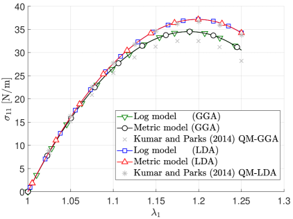
(a)

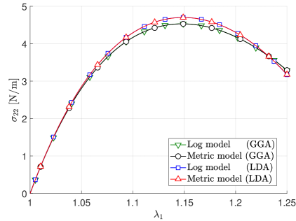
(b)

Figure 2: Uniaxial stretch in the armchair direction: Comparison of the log model [1] and the metric model (proposed here): (2(a)) Stress in the stretched direction; (2(b)) stress in the perpendicular direction. The maximum relative error for $\sigma_{11}$ and $\sigma_{22}$ are 0.019 and 0.199 percent. The quantum mechanical results are taken from Kumar and Parks [2].

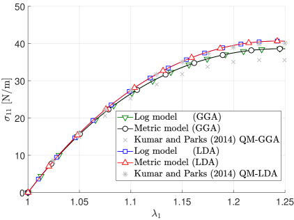
(a)

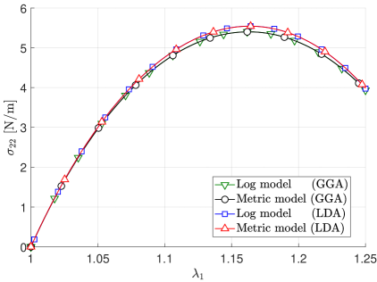
(b)

Figure 3: Uniaxial stretch in the zigzag direction: Comparison of the log model [1] and the metric model (proposed here): (3(a)) Stress in the stretched direction; (3(b)) stress in the perpendicular direction. The maximum relative error for $\sigma_{11}$ and $\sigma_{22}$ are 0.019 and 0.194 percent. The quantum mechanical results are taken from Kumar and Parks [2].

For pure shear, the sheet is pulled in one direction and compressed in the perpendicular direction. The Cartesian components of the stress in the pulled direction, $\sigma_{11}$, and compressed direction, $\sigma_{22}$, are presented in Figs. 4(a) and 4(b) for the GGA parameter set, and in Figs. 5(a) and 5(b) for the LDA parameter set. The stress in the pulled and compressed directions are monolithically increasing or decreasing. The boundary conditions and loads are discussed in more detail in Ghaffari et al. [1].
The results of the metric model for all tests in Figs. 2-5 are in excellent agreement with the log model of Ghaffari et al. [1]. The metric model has the same pure dilatation and bending strain energy density terms as the log model of Ghaffari et al. [1], so there is no need to verify pure dilatation and bending. Note that in general, graphene sheets can wrinkle under uniaxial stretching and shearing, which is avoided here by constraining the out-of-plane deformation.

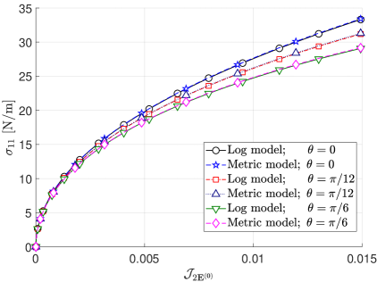
(a)

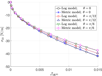
(b)

Figure 4: Pure shear based on the GGA material parameters (see Tab. 2): Comparison of the log model [1] and the metric model (proposed here): (4(a)) Stress in the pull direction; (4(b)) stress in the compression direction. The maximum relative error for $\sigma_{11}$ and $\sigma_{22}$ are 0.35 and 0.42 percent. $\theta$ denotes the direction of pulling relative to the armchair direction.

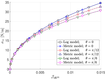
(a)

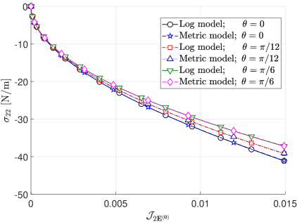
(b)

Figure 5: Pure shear based on the LDA material parameters (see Tab. 2): Comparison of the log model [1] and the metric model (proposed here): (5(a)) Stress in the pull direction; (5(b)) stress in the compression direction. The maximum relative error for $\sigma_{11}$ and $\sigma_{22}$ are 0.12 and 0.22 percent. $\theta$ denotes the direction of pulling relative to the armchair direction.

5 Numerical examples

In this section, the performance of the model is investigated by several examples. The examples are contact of a CNT and CNC with a Lennard-Jones wall and bending and twisting of CNTs and CNCs. Before applying these deformations, the CNT and CNC need to be relaxed, since they can contain residual stresses coming from the rolling of graphene. The strain energy and internal stresses of CNTs and CNCs are minimized initially, before applying the loading. In all examples, the buckling and post-buckling behavior of the structures is computed and the point of buckling can be either determined by examining the ratio of the membrane energy to the total energy or it can be determined from sharp variations in the reaction forces. The modified arc-length method of Ghaffari et al. [78] and a line-search [79, 59, 80, 81] are used to obtain convergence around the buckling point and capture the jump in the energy and force. The simulations will not converge without these methods even when using very small load steps. In the following examples the error is defined by

$$\begin{array}[]{lll}\text{error}\!\!\!&=&\!\!\!\displaystyle\frac{\|q-q_{\text{ref}}\|}{\|q_{\text{ref}}\|}{}\end{array}$$ (40)

where $q$ can be a force or an energy, and $q_{\text{ref}}$ is a corresponding reference value. For comparison of log and metric models, the log model is considered as $q_{\text{ref}}$, and for other examples the metric model with the finest mesh is used as reference. The current formulation does not use any special treatment against locking. Instead, sufficiently fine quadratic NURBS meshes are used.

5.1 Carbon nanotubes

CNT($n,m$) can be generated by rolling a graphene sheet perpendicular to the lattice vector of ($n,m$), where $n$ and $m$ are the chirality parameters [29]. In this section, bending, twisting of CNTs and contact a CNT with a Lennard-Lones wall is considered, and their buckling and postbuckling behavior are simulated. The buckling point can be determined accurately by examining the ratio of the membrane energy to the total energy. At the bucking point membrane energy is converted to bending energy. These points have been obtained for bending and twisting of CNTs in Ghaffari et al. [1].

5.1.1 CNT bending

First, bending of a CNT is considered as shown in Fig. 6(a). The end faces of the CNT are assumed to be rigid and remain planar, and the CNT is allowed to deform in the axial direction in order to avoid a net axial force. The bending angle $\theta$ is applied at both faces of the CNT equally. The variation of the strain energy per atom with the bending angle is shown in Fig. 6(b) and compared with the results of the log model of Ghaffari et al. [1] for perfect and imperfect structures. The imperfection is applied as a small torque in the middle of the CNT. The results of the metric and log models match perfectly. $200\times 200$ quadratic NURBS elements are used in this study. This discretization has an energy error of less than 0.1% as the convergence study in Ghaffari et al. [1] shows.

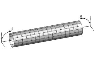
(a)

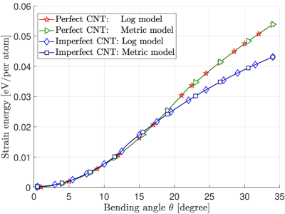
(b)

Figure 6: CNT bending: (6(a)) boundary conditions; (6(b)) strain energy per atom. CNT(10,10) with the length 10 nm is selected. Using Eq. (40), the maximum error relative to the logarithmic model is $7.6500\times 10^{-4}$ percent.

5.1.2 CNT twisting

Next, twisting of a CNT is considered by applying a twisting angle at both faces of the CNT (Fig. 7(a)). The variation of the strain energy per atom with the twisting angle is shown in Fig. 7(b) and compared with the results of the log model of Ghaffari et al. [1].

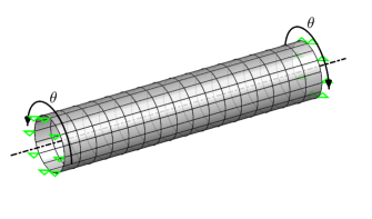
(a)

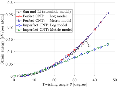
(b)

Figure 7: CNT twisting: (7(a)) boundary conditions (length in the axially direction is fixed); (7(b)) strain energy per atom. CNT(12,6) with the length 6.74 nm is used. The atomistic results are taken from Sun and Li [82]. Using Eq. (40), the maximum error relative to logarithmic model is 0.002 percent.

The results of the metric and log models match up to 0.002%. $100\times 100$ quadratic NURBS elements are used in this study. This discretization has an energy error of less than 0.01% as the convergence study in [1] shows.

5.1.3 CNT contact

Finally, the contact of a CNT with a Lennard-Jones wall is simulated. This is interesting, since a CNT can be used as a tip of an atomic force microscope (AFM). CNTs can have a set of discrete chiralities and radii so they can be mass-produced with a precise radius and length while silicon and silicon nitride tips can not be produced with an identical geometry [83]. This unique feature of CNT-based AFMs guarantees the reproducibility of measurements and experiments with different AFMs [84, 85, 86, 87, 88]. In addition, CNTs-based AFMs have a higher resolution relative to AFMs with silicon or silicon nitride tips [89]. However, the measurement with the AFM is not reliable after buckling and hence buckling should be avoided. A CNT with a larger radius is more stable, but the precision and resolution of the AFM decrease.
Here we study contact and buckling of a CNT with a rigid wall using the setup shown in Fig. 8(a). The wall is modeled with a coarse grained contact model (CGCM) [90, 91, 92, 93, 78]. Within this model, an equivalent half space potential is used at each contact point. This potential can be written as [1]

$$\begin{array}[]{lll}\Psi_{\text{(VdW)h}}\!\!\!&=&\!\!\!\displaystyle-\Gamma\left[\frac{3}{2}\left(\frac{h_{0}}{r}\right)^{3}-\frac{1}{2}\left(\frac{h_{0}}{r}\right)^{9}\right]~{},\end{array}$$ (41)

where $h_{0}=0.34~{}\text{nm}$, $\Gamma=0.14~{}\text{N/m}$ and $r$ are the equilibrium distance, the interfacial adhesion energy per unit area and the normal distance of a surface point to the wall. The wall is moved in the axial direction toward the CNT (during loading) and away from it (during unloading). The results converge with mesh refinement as the error plot based on Eq. (40) in Fig. 8(b) shows. Quadratic NURBS meshes with $32\times 12$, $80\times 30$, $160\times 60$ and $320\times 120$ elements are used for the convergence study. The difference in the wall reaction between the finest and second finest mesh is $7.45\%$.

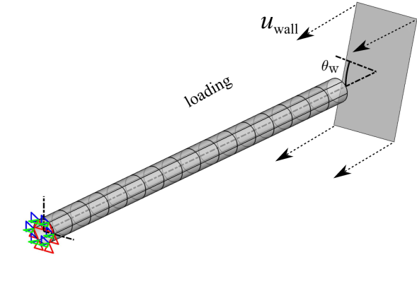
(a)

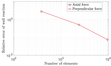
(b)

Figure 8: Contact of a CNT with a Lennard-Jones wall: (8(a)) boundary conditions; (8(b)) Error of the reaction force relative to the finest mesh ($320\times 120$ quadratic NURBS elements). CNT(15,15) with the length 38.19 nm and the contact angle $\theta_{\text{w}}=17.45^{\circ}$ is used.

The contact force is compared with the atomistic results of Schmidt et al. [94] in Fig. 9a. The contact force is also compared to an analytical solution (see D). The extremum of the axial and perpendicular forces are $1.21$ nN and –0.38 nN, respectively. The CNT buckles during loading which leads to a sharp drop in the contact force. This discontinuity is captured by using the arc-length method of Ghaffari et al. [78] in conjugation with a line-search method. During unloading, the reaction force is different than during loading. Note that there are two instabilities 1. buckling / unbuckling (at point B & C in Fig. 9(b)) 2. jump-to- / jump-off-contact (at point A & D in Fig. 9(b)). The second is also common to other adhesive systems at small length scales [95, 96]. The deformed CNT is shown before and after buckling and jump-to / jump-off-contact in Fig. 10.

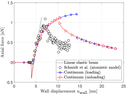
(a)

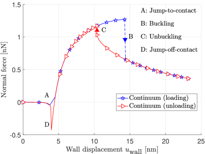
(b)

Figure 9: Contact of a CNT with a the Lennard-Jones wall: Reaction force of the wall in the (9(a)) undeformed axial direction of the CNT (9(b)) normal direction of the wall. CNT(15,15) with the length 38.19 nm and the contact angle $\theta_{\text{w}}=17.45^{\circ}$ is used. The atomistic results are taken from Schmidt et al. [94]${}^{\text{a}}$. The atomistic simulation is conducted at finite temperature but thermal effects are not considered in the continuum model. The relation between axial force $F_{\text{A}}$ and normal force $F_{\text{N}}$ is $F_{\text{N}}=F_{\text{A}}/\cos(\theta_{\text{w}})$. The data between markers is continuous. ${}^{\text{a}}$ The force unit in Schmidt et al. [94] should be nN instead of eV/$\AA$.

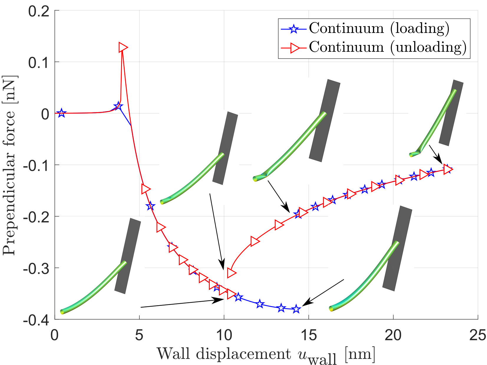
Figure 10: Contact of a CNT with a Lennard-Jones wall: Deformed geometries during loading and unloading.

5.2 Carbon nanocones

A CNC($\theta_{\text{apex}}$) can be generated by rolling a sector of a graphene sheet. It is described with an apex angle $\theta_{\text{apex}}$ and length $L$ (see Fig. 11(a)). A zigzag (or armchair) line can only be matched with another zigzag (or armchair) line to create a CNC (see Fig. 11b). A CNC can be generated from a sector of a graphene sheet that is cut with the declination angle $d_{\theta}$ of $60^{\circ}$, $120^{\circ}$, $180^{\circ}$, $240^{\circ}$ and $300^{\circ}$. Thus $\theta_{\text{apex}}$ can have the discrete values [29, 97]

$$\begin{array}[]{lll}\theta_{\text{apex}}\!\!\!&=&\!\!\!2\,\arcsin(1-d_{\theta}/360)~{}.\end{array}$$ (42)

(a)

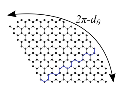
(b)

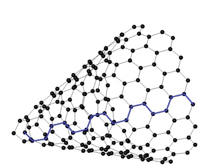
(c)

Figure 11: CNC geometry and lattice: (11(a)) CNC dimensions; (11(b)) flat graphene sheet; (11(c)) rolled graphene sheet. The armchair direction is shown by a blue line.

Similar to the preceding CNT examples, bending, twisting and wall contact of CNCs are considered in the following. It is seen that CNCs buckle without applying an imperfection due to the variation of the chirality along the different tangential coordinates.

5.2.1 CNC bending

The first example considers CNC bending. The boundary conditions for CNC bending are shown in Fig. 12(a). The end faces of the CNC are kept rigid and the bending angle is applied to them equally. Here, the CNC can deform in the axial direction to avoid net axial loading. Fig. 12(b) demonstrates the FE convergence under mesh refinement by examining the error from Eq. (40), where $q_{\text{ref}}$ is the result from the finest mesh. Quadratic NURBS meshes with $m\times m$ elements, for $m$ = 10, 20, 40, 60, 80, 100, 120, are used for the convergence study. The energy difference between the finest and second finest mesh is below $0.38\%$.

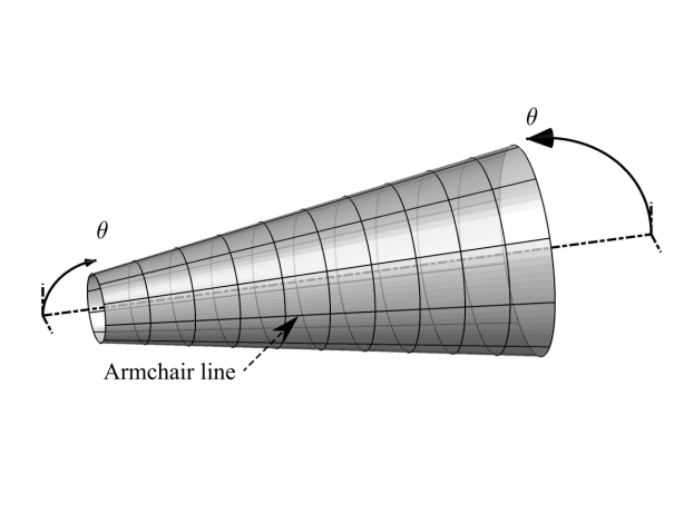
(a)

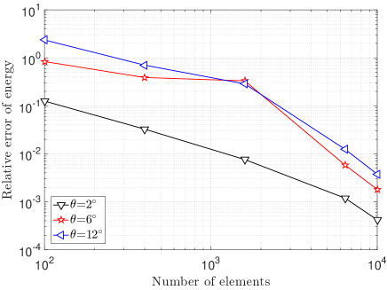
(b)

Figure 12: CNC bending: (12(a)) boundary conditions; (12(b)) Error of strain energy relative to the finest mesh (using $120\times 120$ quadratic NURBS elements). CNC($19.2^{\circ}$) with the length and tip radius 12.04 nm and 1 nm is used.

The strain energy per atom and the ratio of the membrane energy to the total energy as a function of the bending angle are given in Figs. 13(a) and 13(b). The structure buckles at two loading levels: At $\theta=3.48^{\circ}$ the CNC buckles at the tip, and at $\theta=3.9^{\circ}$ the CNC buckles at end. These buckling points can be precisely obtained from the ratio of the membrane energy to the total energy (see Fig. 13(b)). Fig. 14 shows the deformation and stress invariant $\mathrm{tr}\,(\mbox{\boldmath$\sigma$}_{\text{KL}})=\mbox{\boldmath$\sigma$}_{\text{KL}}:\boldsymbol{1}$ following from Eq. (1) at different bending angles.

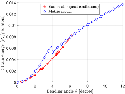
(a)

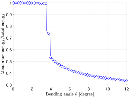
(b)

Figure 13: CNC bending: (13(a)) Comparison of strain energy per atom for the proposed metric model and the quasi-continuum model of Yan et al. [36]; (13(b)) the ratio of the membrane energy to the total energy for the metric model. CNC($19.2^{\circ}$) with the length and tip radius 12.04 nm and 1 nm is used.

Figure 14: CNC bending: Comparison of $\mathrm{tr}\,(\mbox{\boldmath$\sigma$}_{\text{KL}})$ [N/m] at the bending angles (a) $\theta=2^{\circ}$, (b) $\theta=3.5^{\circ}$, (c) $\theta=4^{\circ}$ and (d) $\theta=6^{\circ}$, (e) $\theta=8^{\circ}$, (f) $\theta=12^{\circ}$. CNC($19.2^{\circ}$) with the length and tip radius 12.04 nm and 1 nm is used.

5.2.2 CNC twisting

The second example considers CNC twisting. The boundary conditions of twisting are shown in Fig. 15(a). The end faces of the CNC is kept rigid, the torsion angle is applied to them equally and its length is kept fix. Fig. 15(b) demonstrates the FE convergence under mesh refinement examining the error measure of Eq. (40). Quadratic NURBS meshes with $m\times m$ elements, for m = 10, 20, 40, 80, 100, 120, 140, 160, 200, are used for the convergence study. The energy difference between the finest and second finest mesh is about $0.01\%$.

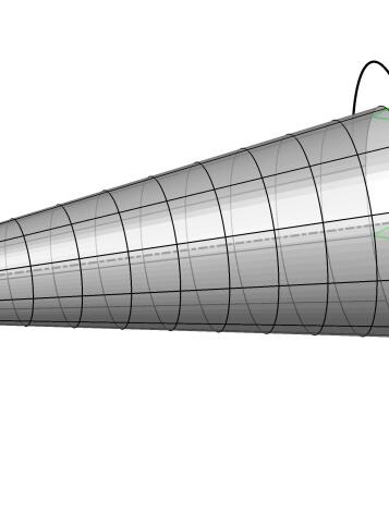
(a)

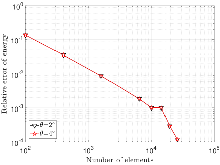
(b)

Figure 15: CNC twisting: (15(a)) boundary conditions; (15(b)) Error of strain energy relative to the finest mesh (using $180\times 180$ quadratic NURBS elements). CNC($19.2^{\circ}$) with the length and tip radius 12.04 nm and 1 nm is used.

The strain energy per atom and the ratio of the membrane energy to the total energy as a function of the twisting angle are given in Figs. 16(a) and 16(b). The structure buckles around $\theta=7^{\circ}$ and $\theta=9.85^{\circ}$, and these points can be precisely obtained from the ratio of the membrane energy to the total energy (see Fig. 16(b)). Two stable paths appear after the second buckling point and the path with the lower level of energy is more favorable (see Wriggers [81] for a discussion of bifurcation in FE analysis). The deformation follows one of the two paths depending on the load step and arclength parameter. Thermal fluctuations at finite temperatures should be sufficient to provide the model with enough energy to overcome the energy barrier between the two paths and go from the higher energy level to the lower one. $\mathrm{tr}\,(\mbox{\boldmath$\sigma$}_{\text{K}})$ is shown at different twisting angles in side and front views in Figs. 17 and 18, respectively. The buckling geometry has rotational symmetry of 180^∘ at low twisting angle (below $\theta=10^{\circ}$) and 120^∘ at high twisting angle (above $\theta=10^{\circ}$) (see Fig. 18c-d).

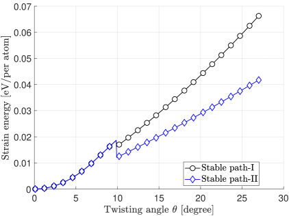
(a)

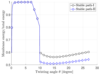
(b)

Figure 16: CNC twisting: (16(a)) Strain energy per atom; (16(b)) the ratio of the membrane energy to the total energy. CNC($19.2^{\circ}$) with the length and tip radius 12.04 nm and 1 nm is used.

Figure 17: CNC twisting: Comparison of tr($\mbox{\boldmath$\sigma$}_{\text{KL}}$) [N/m] at the twisting angles (side view) (a) $\theta=4^{\circ}$, (b) $\theta=7.5^{\circ}$, (c) $\theta=9^{\circ}$ and (d) $\theta=15^{\circ}$, (e) $\theta=20^{\circ}$, (f) $\theta=28.35^{\circ}$. CNC($19.2^{\circ}$) with the length 12.04 nm is used.

Figure 18: CNC twisting: Comparison of tr($\mbox{\boldmath$\sigma$}_{\text{KL}}$) [N/m] at the twisting angles (front view) (a) $\theta=4^{\circ}$, (b) $\theta=7.5^{\circ}$, (c) $\theta=9^{\circ}$ and (d) $\theta=15^{\circ}$, (e) $\theta=20^{\circ}$, (f) $\theta=28.35^{\circ}$. CNC($19.2^{\circ}$) with the length and tip radius 12.04 nm and 1 nm is used.

5.2.3 CNC contact

CNTs are good candidates for AFM tips, but they buckle fast due to their high aspect ratio. Therefore, CNCs are better candidates for AFM tips [98, 99]. To illustrate this point, contact between a CNC and a rigid wall is considered here. In order to compare CNC and CNT, the length and tip radius $r_{\text{tip}}$ of the CNC are selected such that they are equal to the length and radius of the CNT used before. In this case they would be able to measure with the same resolution. The boundary conditions and the deformed geometry of the CNC are shown in Figs. 19(a) and 19(b), respectively. The CNC is simply supported and the wall is rigid and moves in the axial direction of the CNC. The normal contact force is given in Fig. 20. It reaches about 23.41 nN at the buckling point. The buckling force of the CNC is several times larger than the buckling force of the CNT (see Tab. 4). The contact force decreases sharply after the buckling point. Then, it decreases smoothly to a local minimum and begins to increase after that minimum. The buckling force of the CNC is 18.44 times larger than for the CNT. $250\times 150$ quadratic NURBS elements are used in this study.

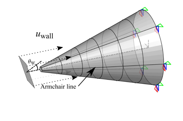
(a)

(b)

Figure 19: Contact of a CNC with a Lennard-Jones wall: (19(a)) boundary conditions; (19(b)) deformed geometry colored with tr($\mbox{\boldmath$\sigma$}_{\text{KL}}$) [N/m]. CNC($38.94^{\circ}$) with the length 38.19 nm and the contact angle $\theta_{\text{w}}=17.45^{\circ}$ are used.

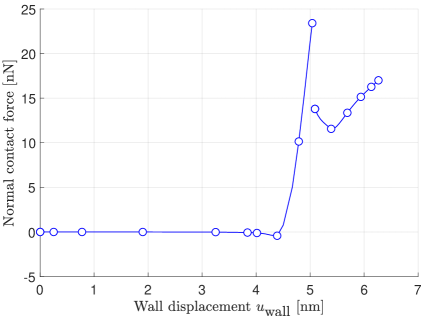
Figure 20: Contact of a CNC with a Lennard-Jones wall: Normal contact force of the wall. CNC($38.94^{\circ}$) with the length 38.19 nm and $\theta_{\text{w}}=17.45^{\circ}$ is used. The data between markers is continuous.

	CNT	CNCs
Normal contact force [nN]	1.27	23.40

Table 4: Comparison of the buckling force for the CNT and CNC considered in Secs. 5.1.3 and 5.2.3 (see Fig. 9 and Fig. 20), respectively.

6 Conclusion

A new hyperelastic material model is proposed for graphene-based structures. The symmetry group and the structural tensor of graphene are used to obtain a set of invariants. These invariants are directly based on the right surface Cauchy-Green deformation tensor $\boldsymbol{C}$, so its derivatives with respect to $\boldsymbol{C}$ can be taken easily. The first and second invariants capture pure dilatation and shear, while the third one captures anisotropic behavior. This model is based on existing quantum data [75, 2]. The speedup of the model is 1.5 compared to the earlier model of Ghaffari et al. [1]. Further, it is simpler to implement than the model of Ghaffari et al. [1]. The material model is formulated such that it can be easily implemented within the rotation-free isogeometric shell formulation of Duong et al. [53]. The elementary behavior of the new model is validated by uniaxial tension and pure shear tests. The strain energy of CNTs and CNCs under bending and twisting are computed. The buckling points are calculated by examining the ratio of membrane energy to total energy. The postbuckling behavior of CNTs and CNCs are simulated. The modified arclength method of Ghaffari et al. [78] and a line search method are used to obtain convergence, and the finite element formulation fails to converge for some of the examples without these methods. CNCs buckle even without applying an imperfection due to inherent anisotropy along the different tangential coordinates. CNTs and CNCs can be used for an atomic force microscope (AFM) tip. Contact of a CNT and CNC with a Lennard-Jones wall is simulated. The reaction forces are computed and it is shown that loading and unloading paths are different for contact of the CNT with the Lennard-Jones wall. A CNT and CNC with the same tip radius are selected so they would have the same measurement precision. It is shown that the buckling force of the CNC is 18.44 times larger than the buckling force of the CNT. Hence, CNCs are much better candidates for AFM tips than CNTs.
The proposed model is obtained from recent ab-intio results and is thus very accurate. MD and multiscale methods based on the first and second Brenner potential on the other hand usually underestimate the elastic modulus by one-third (see Cao [67] and Ghaffari et al. [1] for a comparison of elastic moduli obtained from different potentials). More accurate potentials such as MM3 and REBO+LJ should be used to resolve this inaccuracy. This will be considered in future work.

Appendix A Kinematics of deforming surfaces

Here, the curvilinear description of deforming surfaces is summarized following [52]. The surface in the reference and the current configuration can be written as

$$\begin{array}[]{l}\boldsymbol{X}=\displaystyle\boldsymbol{X}(\xi^{\alpha})~{},\end{array}$$ (43)

$$\begin{array}[]{l}\boldsymbol{x}=\displaystyle\boldsymbol{x}(\xi^{\alpha})~{},\end{array}$$ (44)

where $\xi^{\alpha}$ ($\alpha=1,2$) are the parametric coordinates. The tangent vectors of the reference and current configuration are

$$\begin{array}[]{l}\boldsymbol{A}_{\alpha}=\displaystyle\frac{\partial{\boldsymbol{X}}}{\partial{\xi^{\alpha}}}~{},\end{array}$$ (45)

$$\begin{array}[]{l}\boldsymbol{a}_{\alpha}=\displaystyle\frac{\partial{\boldsymbol{x}}}{\partial{\xi^{\alpha}}}~{}.\end{array}$$ (46)

The co-variant components of the metric tensors are defined by using the inner product as

$$\begin{array}[]{l}A_{\alpha\beta}=\boldsymbol{A}_{\alpha}\cdot\boldsymbol{A}_{\beta}~{},\end{array}$$ (47)

$$\begin{array}[]{l}a_{\alpha\beta}=\boldsymbol{a}_{\alpha}\cdot\boldsymbol{a}_{\beta}~{}.\end{array}$$ (48)

The contra-variant components of the metric tensors are defined as

$$\begin{array}[]{l}[A^{\alpha\beta}]=[A_{\alpha\beta}]^{-1}~{},\end{array}$$ (49)

$$\begin{array}[]{l}[a^{\alpha\beta}]=[a_{\alpha\beta}]^{-1}~{}.\end{array}$$ (50)

The dual tangent vectors can then be defined as

$$\begin{array}[]{lll}\boldsymbol{A}^{\alpha}\!\!\!&:=&\!\!\!A^{\alpha\beta}\,\boldsymbol{A}_{\beta}~{},\end{array}$$ (51)

$$\begin{array}[]{lll}\boldsymbol{a}^{\alpha}\!\!\!&:=&\!\!\!a^{\alpha\beta}\,\boldsymbol{a}_{\beta}~{}.\end{array}$$ (52)

The normal unit vector of the surface in the reference and current configuration can be obtained by using the cross product of the tangent vectors as

$$\begin{array}[]{l}\boldsymbol{N}=\displaystyle\frac{\boldsymbol{A}_{1}\times\boldsymbol{A}_{2}}{\|\boldsymbol{A}_{1}\times\boldsymbol{A}_{2}\|}~{},\end{array}$$ (53)

$$\begin{array}[]{l}\boldsymbol{n}=\displaystyle\frac{\boldsymbol{a}_{1}\times\boldsymbol{a}_{2}}{\|\boldsymbol{a}_{1}\times\boldsymbol{a}_{2}\|}~{}.\end{array}$$ (54)

The 3D identity tensor $\boldsymbol{1}$ can be then written as

$$\begin{array}[]{l}\boldsymbol{1}=\boldsymbol{I}+\boldsymbol{N}\otimes\boldsymbol{N}=\boldsymbol{i}+\boldsymbol{n}\otimes\boldsymbol{n}~{},\end{array}$$ (55)

where $\boldsymbol{I}$ and $\boldsymbol{i}$ are the surface identity tensor in the reference and current configuration. They are

$$\begin{array}[]{l}\boldsymbol{I}=\boldsymbol{A}_{\alpha}\otimes\boldsymbol{A}^{\alpha}=A_{\alpha\beta}\,\boldsymbol{A}^{\alpha}\otimes\boldsymbol{A}^{\beta}=A^{\alpha\beta}\,\boldsymbol{A}_{\alpha}\otimes\boldsymbol{A}_{\beta}~{},\end{array}$$ (56)

$$\begin{array}[]{l}\boldsymbol{i}=\boldsymbol{a}_{\alpha}\otimes\boldsymbol{a}^{\alpha}=a_{\alpha\beta}\,\boldsymbol{a}^{\alpha}\otimes\boldsymbol{a}^{\beta}=a^{\alpha\beta}\,\boldsymbol{a}_{\alpha}\otimes\boldsymbol{a}_{\beta}~{}.\end{array}$$ (57)

The co-variant components of the curvature tensor are defined as

$$\begin{array}[]{l}b_{\alpha\beta}:=\boldsymbol{n}\cdot\boldsymbol{a}_{\alpha,\beta}=\boldsymbol{n}\cdot\boldsymbol{a}_{\alpha;\beta}~{},\end{array}$$ (58)

where $\boldsymbol{a}_{\alpha,\beta}$ and $\boldsymbol{a}_{\alpha;\beta}$ are the parametric and co-variant derivatives of the tangent vectors. They are connected by

$$\begin{array}[]{l}\boldsymbol{a}_{\alpha;\beta}=\boldsymbol{a}_{\alpha,\beta}-\Gamma^{\gamma}_{\alpha\beta}\,\boldsymbol{a}_{\gamma}~{},\end{array}$$ (59)

where $\Gamma^{\gamma}_{\alpha\beta}$ is the Christoffel symbol of the second kind. It is defined as

$$\begin{array}[]{lll}\Gamma^{\gamma}_{\alpha\beta}\ \!\!\!&:=&\!\!\!\boldsymbol{a}_{\alpha,\beta}\cdot\boldsymbol{a}^{\gamma}~{}.\end{array}$$ (60)

The mixed and contra-variant components of the curvature tensor, $b_{\alpha}^{\beta}$ and $b^{\alpha\beta}$, are defined as

$$\begin{array}[]{lll}b_{\alpha}^{\beta}\!\!\!&=&\!\!\!b_{\alpha\gamma}\,a^{\gamma\beta}~{},\\[8.53581pt] b^{\alpha\beta}\!\!\!&:=&\!\!\!a^{\alpha\gamma}\,b_{\gamma\delta}\,a^{\delta\beta}~{}.\end{array}$$ (61)

The mean and Gaussian curvatures are defined as

$$\begin{array}[]{l}H:=\displaystyle\frac{1}{2}b^{\alpha}_{\alpha}=\frac{1}{2}(\kappa_{1}+\kappa_{2})~{},\end{array}$$ (62)

$$\begin{array}[]{l}\kappa:=\displaystyle\frac{\det[b_{\alpha\beta}]}{\det[a_{\gamma\delta}]}=\kappa_{1}\,\kappa_{2}~{},\end{array}$$ (63)

where $\kappa_{\alpha}$ are the principal curvatures that follow as the eigenvalues of matrix $\left[b_{\alpha}^{\beta}\right]$.

Appendix B Symmetry group and material invariants

In this section, the structural tensor for structures with $n$-fold rotational symmetry are reviewed. Two set of invariants are introduced by using the introduced structural tensor. They are based on the logarithmic strain tensor, following Kumar and Parks [2], and a new set based on the right Cauchy-Green deformation tensor.

B.1 Structural tensor of $C_{nv}$

A 2D structure can be modeled based on its lattice structure and symmetry group. A symmetry group is a certain type of operations that leave the lattice indistinguishable from its initial configuration [100]. The usual operations are identity mapping, inversion, rotation and reflection. They can be used to formulate structural tensors for the modeling of anisotropic materials [47]. The structural tensors of a lattice with symmetry group of $n$-fold rotational symmetry and additional reflection plane $C_{nv}$ are given as [47]

$$\begin{array}[]{lll}\displaystyle\mathbb{H}_{n}\!\!\!&:=&\!\!\!\Re\left[(\hat{\boldsymbol{x}}+i\hat{\boldsymbol{y}})^{(n)}\right]=\left\{{\begin{array}[]{*{20}{l}}{\Re\left[\left(\hat{\boldsymbol{M}}+i\hat{\boldsymbol{N}}\right)^{(m)}\right];~{}~{}n=2m}~{},\\[14.22636pt] {\Re\left[\left(\hat{\boldsymbol{x}}+i\hat{\boldsymbol{y}}\right)\otimes\left(\hat{\boldsymbol{M}}+i\hat{\boldsymbol{N}}\right)^{(m)}\right];~{}~{}n=2m+1~{},}\end{array}}\right.\end{array}$$ (64)

where $\hat{\boldsymbol{x}}$ and $\hat{\boldsymbol{y}}$ are two orthonormal vectors (see Fig. 1) and at least one of them is in the crystal symmetry plane, $i$ is the imaginary unit number, $(\bullet)^{(n)}:=(\bullet)\otimes(\bullet)...(\bullet)$ is the tensor product of $n$ times, $m$ is a integer number, $\Re$ indicates real part of its argument, and $\hat{\boldsymbol{M}}$ and $\hat{\boldsymbol{N}}$ are defined as

$$\begin{array}[]{lll}\hat{\boldsymbol{M}}\!\!\!&:=&\!\!\!\hat{\boldsymbol{x}}\,\otimes\,\hat{\boldsymbol{x}}-\hat{\boldsymbol{y}}\,\otimes\,\hat{\boldsymbol{y}}~{},\\[5.69054pt] \hat{\boldsymbol{N}}\!\!\!&:=&\!\!\!\hat{\boldsymbol{x}}\,\otimes\,\hat{\boldsymbol{y}}+\hat{\boldsymbol{y}}\,\otimes\,\hat{\boldsymbol{x}}~{}.\end{array}$$ (65)

Graphene has a hexagonal lattice and its structure repeats after $60^{\circ}$ of rotation. This lattice relates to the symmetry group of $C_{nv}$ and has 14 symmetry operations, which are an identity mapping, an inversion, six mirror planes and six rotations. $\hat{\boldsymbol{x}}$ taken in the armchair direction (see Fig. 1) and $n=6$ for graphene. Directions of $\hat{\boldsymbol{x}}$ and $\hat{\boldsymbol{y}}$ can be transformed to $\hat{\boldsymbol{x}}^{\diamond}$ and $\hat{\boldsymbol{y}}^{\diamond}$ by a rotation of $\theta$ in the counter-clock-wise direction such that

$$\begin{array}[]{lll}\displaystyle\hat{\boldsymbol{x}}^{\diamond}+i\,\hat{\boldsymbol{y}}^{\diamond}\!\!\!&=&\!\!\!e^{-i\,\theta}\left(\hat{\bf{x}}+i\,\hat{\bf{y}}\right)~{},\\[5.69054pt] \hat{\boldsymbol{M}}^{\diamond}+i\,\hat{\boldsymbol{N}}^{\diamond}\!\!\!&=&\!\!\!\displaystyle e^{-2\,i\,\theta}\left(\hat{\boldsymbol{M}}+i\,\hat{\boldsymbol{N}}\right)~{},\\[5.69054pt] \displaystyle\mathbb{H}_{n}\!\!\!&=&\!\!\!\displaystyle\left[\hat{\boldsymbol{M}}\,\otimes\,\hat{\boldsymbol{M}}\,\otimes\,\hat{\boldsymbol{M}}-\left(\hat{\boldsymbol{M}}\,\otimes\,\hat{\boldsymbol{N}}\,\otimes\,\hat{\boldsymbol{N}}+\hat{\boldsymbol{N}}\,\otimes\,\hat{\boldsymbol{M}}\,\otimes\,\hat{\boldsymbol{N}}+\hat{\boldsymbol{N}}\,\otimes\,\hat{\boldsymbol{N}}\,\otimes\,\hat{\boldsymbol{M}}\right)\right]\\[5.69054pt] \!\!\!&=&\!\!\!\displaystyle\Re\left[{e^{i\,n\,\theta}\left(\hat{\boldsymbol{x}}^{\diamond}+i\hat{\boldsymbol{y}}^{\diamond}\right)^{(n)}}\right]~{}.\end{array}$$ (66)

The invariants of a symmetric surface tensor of rank 2 $\boldsymbol{A}$ $\in\mathbb{R}^{3}\times\mathbb{R}^{3}$ can be written as [47, 48]

$$\begin{array}[]{lll}\displaystyle\mathcal{J}_{1\boldsymbol{A}}^{\vdash}\!\!\!&=&\!\!\!\displaystyle\mathrm{tr}\,(\boldsymbol{A})~{},\\[5.69054pt] \displaystyle\bar{\mathcal{J}}_{2\boldsymbol{A}}^{\vdash}\!\!\!&=&\!\!\!\displaystyle\frac{1}{2}\,\mathrm{tr}\,\left(\boldsymbol{A}^{2}\right)~{},\\[5.69054pt] \mathcal{J}_{3\boldsymbol{A}}^{\vdash}\!\!\!&=&\!\!\!\displaystyle\frac{1}{8}\mathrm{tr}\,\left(\Pi^{\boldsymbol{A}}_{n}\,\boldsymbol{A}\right)=\frac{1}{8}\Pi^{\boldsymbol{A}}_{n}:\boldsymbol{A}~{},\end{array}$$ (67)

where $\Pi^{\boldsymbol{A}}_{n}$ is defined as

$$\begin{array}[]{lll}\Pi^{\boldsymbol{A}}_{n}\!\!\!&:=&\!\!\!A^{m-1}\,\Re\left[e^{i\,n\,\theta+i\,(m-1)\,\theta_{\boldsymbol{A}}}\left(\hat{\boldsymbol{M}}^{\diamond}+i\,\hat{\boldsymbol{N}}^{\diamond}\right)\right]~{}\text{with}~{}n=2m~{},~{}m=1,2,3,...~{},\end{array}$$ (68)

and $\theta_{\boldsymbol{A}}$ and $A$ can be obtained from

$$\begin{array}[]{lll}2\boldsymbol{A}\!\!\!&=&\!\!\!\mathrm{tr}\,(\boldsymbol{A})\,\boldsymbol{I}+A\,\left[\cos(\theta_{\boldsymbol{A}})\,\hat{\boldsymbol{M}}^{\diamond}+\sin(\theta_{\boldsymbol{A}})\hat{\boldsymbol{N}}^{\diamond}\right]~{}.\end{array}$$ (69)

$\theta_{\boldsymbol{A}}$ and $A$ can be easily obtained by using the spectral decomposition of $\boldsymbol{A}$, i.e

$$\begin{array}[]{lll}\boldsymbol{A}\!\!\!&=&\!\!\!\displaystyle\sum_{\alpha=1}^{2}{\lambda_{\alpha\boldsymbol{A}}\boldsymbol{Y}_{\!\alpha\boldsymbol{A}}\otimes\boldsymbol{Y}_{\!\alpha\boldsymbol{A}}}~{},\end{array}$$ (70)

where $\lambda_{\alpha\boldsymbol{A}}$ and $\boldsymbol{Y}_{\!\alpha\boldsymbol{A}}$ are the eigenvalues and eigenvectors of $\boldsymbol{A}$. If $\theta$ selected such that $\hat{\boldsymbol{x}}^{\diamond}$ and $\boldsymbol{Y}_{\!1\boldsymbol{A}}$ are in the same direction, then $A=\lambda_{1\boldsymbol{A}}-\lambda_{2\boldsymbol{A}};(\lambda_{1\boldsymbol{A}}>\lambda_{2\boldsymbol{A}})$ and $\theta_{\boldsymbol{A}}=0$.

B.2 Invariants based on the logarithmic strain

The logarithmic strain is a good candidate for the development of material models. It can be used to additively decompose finite strains into volumetric/deviatoric and elastic/plastic strains. This additive decomposition simplifies the formulation of constitutive laws. In addition, it can capture micro-mechanical behavior of materials very well [101, 102, 103, 104]. Using Eq. (67), the invariant of the logarithmic strain $\boldsymbol{E}^{(0)}=\ln(\boldsymbol{U})$ can be obtained by taking $\boldsymbol{A}=\boldsymbol{E}^{(0)}$ as

$$\begin{array}[]{lll}\displaystyle\mathcal{J}_{1\boldsymbol{E}^{(0)}}\!\!\!&=&\!\!\!\mathrm{tr}\,\left(\boldsymbol{E}^{(0)}\right)=\ln(\lambda_{1}\,\lambda_{2})=\ln(J)~{},\\[5.69054pt] \displaystyle\mathcal{J}_{2\boldsymbol{E}^{(0)}}^{\vdash}\!\!\!&=&\!\!\!\displaystyle\frac{1}{2}\,\mathrm{tr}\,\left(\left(\boldsymbol{E}^{(0)}\right)^{2}\right)=\frac{1}{2}\,\left(\frac{1}{2}\ln(J)\boldsymbol{I}+\boldsymbol{E}^{(0)}_{\text{dev}}\right):\left(\frac{1}{2}\ln(J)\boldsymbol{I}+\boldsymbol{E}^{(0)}_{\text{dev}}\right)\\[11.38109pt] \!\!\!&=&\!\!\!\displaystyle\frac{1}{4}\ln(J)+\frac{1}{2}\boldsymbol{E}^{(0)}_{\text{dev}}:\boldsymbol{E}^{(0)}_{\text{dev}}~{},\\[5.69054pt] \displaystyle\mathcal{J}_{3\boldsymbol{E}^{(0)}}\!\!\!&=&\!\!\!\displaystyle\frac{1}{8}\mathbb{H}\left(\boldsymbol{E}^{(0)},\boldsymbol{E}^{(0)},\boldsymbol{E}^{(0)}\right)=\left(E^{(0)}\right)^{3}\,\cos(6\theta)=\left(\ln\left(\frac{\lambda_{1}}{\lambda_{2}}\right)\right)^{3}\,\cos(6\theta)~{},\end{array}$$ (71)

where $\lambda_{\alpha}$ are the eigenvalues of the surface stretch tensor and $\boldsymbol{E}^{(0)}_{\text{dev}}=\boldsymbol{E}^{(0)}-1/2\ln(J)\boldsymbol{I}$ is deviatoric part of the strain. These set of invariants can be simplified by eliminating the first invariant from the second invariant as

$$\begin{array}[]{lll}\displaystyle\mathcal{J}_{1\boldsymbol{E}^{(0)}}=\displaystyle\ln(J)~{},\\[5.69054pt] \displaystyle\mathcal{J}_{2\boldsymbol{E}^{(0)}}=\displaystyle\frac{1}{2}\boldsymbol{E}^{(0)}_{\text{dev}}:\boldsymbol{E}^{(0)}_{\text{dev}}=(\ln(\lambda))^{2}~{},\\[5.69054pt] \displaystyle\mathcal{J}_{3\boldsymbol{E}^{(0)}}=\displaystyle\frac{1}{8}\mathbb{H}\left(\boldsymbol{E}^{(0)},\boldsymbol{E}^{(0)},\boldsymbol{E}^{(0)}\right)=(\ln(\lambda))^{3}\,\cos(6\theta)~{},\end{array}$$ (72)

with $\displaystyle\lambda=\sqrt{\frac{\lambda_{1}}{\lambda_{2}}};\lambda_{1}>\lambda_{2}$.

B.3 Invariants based on the right Cauchy-Green tensor

The logarithmic strain facilitates the development of material models and strain energy densities. But for the classical numerical description and FE implementation, derivatives of the strain energy density with respect to $\boldsymbol{C}$ are needed. So, the chain rule should be utilized for material models based on $\boldsymbol{E}^{(0)}$. The first and second derivative are the stress and elasticity tensor. These tensors can be directly obtained for isotropic materials that are developed based on $\boldsymbol{E}^{(0)}$ without using the chain rule [59], but it is not the case for anisotropic materials. Using Eq. (67), a set of invariants based on $\boldsymbol{C}$ can be written as

$$\begin{array}[]{lll}\displaystyle\mathcal{J}_{1\boldsymbol{C}}^{\vdash}\!\!\!&=&\!\!\!\displaystyle\mathrm{tr}\,(\boldsymbol{C})~{},\\[5.69054pt] \displaystyle\mathcal{J}_{2\boldsymbol{C}}^{\vdash}\!\!\!&=&\!\!\!\displaystyle\frac{1}{2}\boldsymbol{C}:\boldsymbol{C}=\frac{1}{2}\left(\Lambda_{1}^{2}+\Lambda_{2}^{2}\right)~{},\\[5.69054pt] \displaystyle\mathcal{J}_{3\boldsymbol{C}}^{\vdash}\!\!\!&=&\!\!\!\displaystyle\frac{1}{8}\mathbb{H}(\boldsymbol{C},\boldsymbol{C},\boldsymbol{C})=\frac{1}{8}\left(\Lambda_{1}-\Lambda_{2}\right)^{3}\,\cos(6\theta)~{}.\end{array}$$ (73)

The material model will be simplified by using a set of invariants which correspond to area-changing and area-invariant deformations. So, $J$ is assumed to be an additional invariant and the set of invariants will be

$$\begin{array}[]{lll}\displaystyle\bar{\mathcal{J}}_{1\boldsymbol{C}}^{\vdash}\!\!\!&=&\!\!\!\displaystyle\mathrm{tr}\,(\bar{\boldsymbol{C}})~{},\\[5.69054pt] \displaystyle\bar{\mathcal{J}}_{2\boldsymbol{C}}^{\vdash}\!\!\!&=&\!\!\!\displaystyle\frac{1}{2}\bar{\boldsymbol{C}}:\bar{\boldsymbol{C}}=\frac{1}{2}\left(\frac{\Lambda_{1}}{\Lambda_{2}}+\frac{\Lambda_{2}}{\Lambda_{1}}\right)~{},\\[5.69054pt] \displaystyle\bar{\mathcal{J}}_{3\boldsymbol{C}}^{\vdash}\!\!\!&=&\!\!\!\displaystyle\frac{1}{8}\mathbb{H}(\bar{\boldsymbol{C}},\bar{\boldsymbol{C}},\bar{\boldsymbol{C}})=\frac{1}{8}\left(\frac{\lambda_{1}}{\lambda_{2}}-\frac{\lambda_{2}}{\lambda_{1}}\right)^{3}\,\cos(6\theta)~{},\\ \bar{\mathcal{J}}_{4\boldsymbol{C}}^{\vdash}\!\!\!&=&\!\!\!J~{},\end{array}$$ (74)

where $\bar{\boldsymbol{C}}$ is the area-invariant part of $\boldsymbol{C}$ which is defined based on the area-invariant deformation gradient $\bar{\boldsymbol{F}}$ (see Eq. (16)). The material model will be more simple, if the set of the invariants are irreducible. $\bar{\mathcal{J}}_{1\boldsymbol{C}}^{\vdash}$ can be written based on $\bar{\mathcal{J}}_{2\boldsymbol{C}}^{\vdash}$ as

$$\begin{array}[]{lll}(\bar{\mathcal{J}}_{1\boldsymbol{C}}^{\vdash})^{2}\!\!\!&=&\!\!\!\displaystyle\frac{1}{2}\bar{\mathcal{J}}_{2\boldsymbol{C}}^{\vdash}+2~{}.\end{array}$$ (75)

So, $\bar{\mathcal{J}}_{1\boldsymbol{C}}^{\vdash}$ is dependent on $\bar{\mathcal{J}}_{2\boldsymbol{C}}^{\vdash}$ and can be excluded from the list of invariants. In addition, $\bar{\mathcal{J}}_{2\boldsymbol{C}}$ can be written as

$$\begin{array}[]{lll}\bar{\mathcal{J}}_{2\boldsymbol{C}}^{\vdash}\!\!\!&=&\!\!\!2\mathcal{J}_{2\boldsymbol{C}}+1~{},\end{array}$$ (76)

where $\mathcal{J}_{2\boldsymbol{C}}$ and the final form of the other invariants are given in Eq. (15).

B.4 Invariants based on the right Cauchy-Green and curvature tensors

A surface can be described by the first and second fundamental forms of the surface, which are the metric and curvature tensors. Hence, the curvature tensor $\boldsymbol{\kappa}$ can be considered as the second tensorial object next to $\boldsymbol{C}$. A set of nine invariants based on $\boldsymbol{C}$ and $\boldsymbol{\kappa}$ can be obtained as

$$\begin{array}[]{lll}\displaystyle\mathcal{J}_{1\boldsymbol{C}}\!\!\!&=&\!\!\!\displaystyle\sqrt{\det(\boldsymbol{C})}=J~{},\\[5.69054pt] \displaystyle\mathcal{J}_{2\boldsymbol{C}}\!\!\!&=&\!\!\!\displaystyle\frac{1}{2}\bar{\boldsymbol{C}}^{\bot}:\bar{\boldsymbol{C}}^{\bot}~{},\\[5.69054pt] \displaystyle\mathcal{J}_{3\boldsymbol{C}}\!\!\!&=&\!\!\!\displaystyle\frac{1}{8}\mathbb{H}\left(\bar{\boldsymbol{C}},\bar{\boldsymbol{C}},\bar{\boldsymbol{C}}\right)=\frac{1}{8}\left(\frac{\lambda_{1}}{\lambda_{2}}-\frac{\lambda_{2}}{\lambda_{1}}\right)^{3}\cos(6\varphi_{\boldsymbol{C}})~{},\\[5.69054pt] \displaystyle\mathcal{J}_{4\boldsymbol{\kappa}}\!\!\!&=&\!\!\!\displaystyle\frac{1}{2}\mathrm{tr}\,(\boldsymbol{\kappa})=H~{},\\[5.69054pt] \mathcal{J}_{5\boldsymbol{\kappa}}\!\!\!&=&\!\!\!\displaystyle\kappa~{},\\[5.69054pt] \mathcal{J}_{6\boldsymbol{\kappa}}\!\!\!&=&\!\!\!\displaystyle\frac{1}{8}\mathbb{H}(\boldsymbol{\kappa},\boldsymbol{\kappa},\boldsymbol{\kappa})=\frac{1}{8}(\kappa_{1}-\kappa_{2})^{3}\cos(6\varphi_{\boldsymbol{\kappa}})~{},\\[5.69054pt] \displaystyle\mathcal{J}_{7\boldsymbol{C}\,\boldsymbol{\kappa}}\!\!\!&=&\!\!\!\displaystyle\frac{1}{2}\bar{\boldsymbol{C}}:\boldsymbol{\kappa}~{},\\[5.69054pt] \displaystyle\mathcal{J}_{8\boldsymbol{C}\,\boldsymbol{\kappa}}\!\!\!&=&\!\!\!\displaystyle\frac{1}{8}\mathbb{H}\left(\bar{\boldsymbol{C}},\bar{\boldsymbol{C}},\boldsymbol{\kappa}\right)=\frac{1}{8}\left(\frac{\lambda_{1}}{\lambda_{2}}-\frac{\lambda_{2}}{\lambda_{1}}\right)^{2}(\kappa_{1}-\kappa_{2})\cos(4\varphi_{\boldsymbol{C}}+2\varphi_{\boldsymbol{\kappa}})~{},\\[5.69054pt] \displaystyle\mathcal{J}_{9\boldsymbol{C}\,\boldsymbol{\kappa}}\!\!\!&=&\!\!\!\displaystyle\frac{1}{8}\mathbb{H}\left(\boldsymbol{\kappa},\boldsymbol{\kappa},\bar{\boldsymbol{C}}\right)=\frac{1}{8}\left(\frac{\lambda_{1}}{\lambda_{2}}-\frac{\lambda_{2}}{\lambda_{1}}\right)(\kappa_{1}-\kappa_{2})^{2}\cos(2\varphi_{\boldsymbol{C}}+4\varphi_{\boldsymbol{\kappa}})~{},\end{array}$$ (77)

where $H$ and $\kappa$ are the mean and Gaussian curvatures and $\kappa_{\alpha}$ are the eigenvalues of the curvature tensor such that $\kappa_{1}>\kappa_{2}$. $\varphi_{\boldsymbol{C}}$ and $\varphi_{\boldsymbol{\kappa}}$ are the angles between the eigenvectors of $\boldsymbol{C}$ and $\boldsymbol{\kappa}$ relative to $\hat{\boldsymbol{x}}$ and are defined as

$$\begin{array}[]{lll}\cos(\varphi_{\boldsymbol{\kappa}})\!\!\!&:=&\!\!\!\hat{\boldsymbol{x}}\cdot\boldsymbol{Y}_{\!1\boldsymbol{\kappa}}~{},\\ \cos(\varphi_{\boldsymbol{C}})\!\!\!&:=&\!\!\!\hat{\boldsymbol{x}}\cdot\boldsymbol{Y}_{\!1\boldsymbol{C}}~{},\end{array}$$ (78)

where $\boldsymbol{Y}_{\!1\boldsymbol{\kappa}}$ and $\boldsymbol{Y}_{\!1\boldsymbol{C}}$ are the eigenvectors of $\boldsymbol{C}$ and $\boldsymbol{\kappa}$ corresponding to the largest eigenvalue. In the current model, the bending energy is assumed to be isotropic.

Appendix C Various derivatives

The derivatives of the invariants of $\boldsymbol{C}=\boldsymbol{F}^{\text{T}}\,\boldsymbol{F}$ can be written as

$$\begin{array}[]{lll}\displaystyle\frac{\partial{\mathcal{J}_{1\boldsymbol{C}}}}{\partial{\boldsymbol{C}}}\!\!\!&=&\!\!\!\displaystyle\frac{1}{2}J\,\boldsymbol{C}^{-1}~{},\\[8.53581pt] \displaystyle\frac{\partial{\mathcal{J}_{2\boldsymbol{C}}}}{\partial{\boldsymbol{C}}}\!\!\!&=&\!\!\!\displaystyle\frac{1}{J}\bar{\boldsymbol{C}}^{\bot}-\mathcal{J}_{2\boldsymbol{C}}\,\boldsymbol{C}^{-1}~{},\\[8.53581pt] \displaystyle\frac{\partial{\mathcal{J}_{3\boldsymbol{C}}}}{\partial{\boldsymbol{C}}}\!\!\!&=&\!\!\!\displaystyle-\frac{3}{2}\mathcal{J}_{3\boldsymbol{C}}\,\boldsymbol{C}^{-1}+\frac{1}{8J}\left[a_{\hat{\boldsymbol{M}}}\,\hat{\boldsymbol{M}}+a_{\hat{\boldsymbol{N}}}\,\hat{\boldsymbol{N}}\right]~{},\end{array}$$ (79)

and derivative of strain energy density as

$$\begin{array}[]{lll}\displaystyle\frac{\partial{W}}{\partial{\mathcal{J}_{1\boldsymbol{C}}}}\!\!\!&=&\!\!\!\displaystyle\frac{\varepsilon}{J}\,\hat{\alpha}^{2}\ln(J)e^{-\hat{\alpha}\ln(J)}+2\mu^{\prime}f_{1}+\eta^{\prime}f_{2}~{},\\[11.38109pt] \displaystyle\frac{\partial{W}}{\partial{\mathcal{J}_{2\boldsymbol{C}}}}\!\!\!&=&\!\!\!\displaystyle 2\mu(e_{1}-2e_{2}\,\mathcal{J}_{2\boldsymbol{C}})-g_{2}\,\eta\,\mathcal{J}_{3\boldsymbol{C}}~{},\\[11.38109pt] \displaystyle\frac{\partial{W}}{\partial{\mathcal{J}_{3\boldsymbol{C}}}}\!\!\!&=&\!\!\!\displaystyle\eta(g_{1}-g_{2}\,\mathcal{J}_{2\boldsymbol{C}})~{},\end{array}$$ (80)

where $\mu^{\prime}$ and $\eta^{\prime}$ are

$$\begin{array}[]{lll}\mu^{\prime}\!\!\!&:=&\!\!\!\displaystyle-\mu_{1}\,\hat{\beta}\,J^{\hat{\beta}-1}~{},\\[5.69054pt] \eta^{\prime}\!\!\!&:=&\!\!\!\displaystyle-2\frac{\eta_{1}}{J}\ln(J)~{}.\end{array}$$ (81)

$H_{i}$ are needed in the computation of the 2.PK stress and its corresponding elasticity tensor, see Eqs. (25) and (26). They are defined as

$$\begin{array}[]{lll}H_{1}\!\!\!&:=&\!\!\!\displaystyle\varepsilon\,\hat{\alpha}^{2}\ln(J)\,e^{-\hat{\alpha}\ln(J)}-2\mu_{1}\,\hat{\beta}\,J^{\hat{\beta}}\,f_{1}-2\eta_{1}\ln(J)\,f_{2}-H_{2}\,\mathcal{J}_{2\boldsymbol{C}}-3H_{3}\,\mathcal{J}_{3\boldsymbol{C}}~{},\\[5.69054pt] H_{2}\!\!\!&:=&\!\!\!\displaystyle 2\left(2\mu(e_{1}-2e_{2}\,\mathcal{J}_{2\boldsymbol{C}})-g_{2}\,\eta\,\mathcal{J}_{3\boldsymbol{C}}\right)~{},\\[5.69054pt] H_{3}\!\!\!&:=&\!\!\!\displaystyle\eta(g_{1}-g_{2}\,\mathcal{J}_{2\boldsymbol{C}})~{},\end{array}$$ (82)

and their derivatives w.r.t. the invariants of $\boldsymbol{C}$ are

$$\begin{array}[]{lll}\displaystyle\frac{\partial{H_{1}}}{\partial{\mathcal{J}_{1\boldsymbol{C}}}}\!\!\!&=&\!\!\!\displaystyle\frac{\varepsilon\,\hat{\alpha}^{2}}{J}\,(1-\hat{\alpha}\,\ln(J))\,e^{-\hat{\alpha}\,\ln(J)}-2\mu_{1}\,\hat{\beta}^{2}\,J^{\hat{\beta}-1}\,f_{1}-2\frac{\eta_{1}}{J}\,f_{2}-\frac{\partial{H_{2}}}{\partial{\mathcal{J}_{1\boldsymbol{C}}}}\mathcal{J}_{2\boldsymbol{C}}-3\frac{\partial{H_{3}}}{\partial{\mathcal{J}_{1\boldsymbol{C}}}}\,\mathcal{J}_{3\boldsymbol{C}}~{},\\[11.38109pt] \displaystyle\frac{\partial{H_{2}}}{\partial{\mathcal{J}_{1\boldsymbol{C}}}}\!\!\!&=&\!\!\!\displaystyle 2\left[2\left(-\mu_{1}\,\hat{\beta}\,J^{\hat{\beta}-1}(e_{1}-2\,e_{2}\,\mathcal{J}_{2\boldsymbol{C}})\right)+2\frac{g_{2}\,\eta_{1}}{J}\,\ln(J)\,\mathcal{J}_{3\boldsymbol{C}}\right]~{},\\[11.38109pt] \displaystyle\frac{\partial{H_{3}}}{\partial{\mathcal{J}_{1\boldsymbol{C}}}}\!\!\!&=&\!\!\!\displaystyle-2\frac{\eta_{1}}{J}\ln(J)\,(g_{1}-g_{2}\,\mathcal{J}_{2\boldsymbol{C}})~{},\end{array}$$ (83)

$$\begin{array}[]{lll}\displaystyle\frac{\partial{H_{1}}}{\partial{\mathcal{J}_{2}}}\!\!\!&=&\!\!\!\displaystyle-2\mu_{1}\,\hat{\beta}\,J^{\hat{\beta}}\,(e_{1}-2\,e_{2}\,\mathcal{J}_{2\boldsymbol{C}})+2g_{2}\,\eta_{1}\,\ln(J)\,\mathcal{J}_{3\boldsymbol{C}}-H_{2}-\frac{\partial{H_{2}}}{\partial{\mathcal{J}_{2\boldsymbol{C}}}}\mathcal{J}_{2\boldsymbol{C}}-3\mathcal{J}_{3\boldsymbol{C}}\,\frac{\partial{H_{3}}}{\partial{\mathcal{J}_{2\boldsymbol{C}}}}~{},\\[11.38109pt] \displaystyle\frac{\partial{H_{2}}}{\partial{\mathcal{J}_{2\boldsymbol{C}}}}\!\!\!&=&\!\!\!\displaystyle-8\mu\,e_{2}~{},\\[11.38109pt] \displaystyle\frac{\partial{H_{3}}}{\partial{\mathcal{J}_{2\boldsymbol{C}}}}\!\!\!&=&\!\!\!\displaystyle-\eta\,g_{2}~{},\end{array}$$ (84)

and

$$\begin{array}[]{lll}\displaystyle\frac{\partial{H_{1}}}{\partial{\mathcal{J}_{3\boldsymbol{C}}}}\!\!\!&=&\!\!\!\displaystyle-2\eta_{1}\,(g_{1}-g_{2}\,\mathcal{J}_{2\boldsymbol{C}})\,\ln(J)-\frac{\partial{H_{2}}}{\partial{\mathcal{J}_{3\boldsymbol{C}}}}\,\mathcal{J}_{2\boldsymbol{C}}-3\,H_{3}~{},\\[11.38109pt] \displaystyle\frac{\partial{H_{2}}}{\partial{\mathcal{J}_{3\boldsymbol{C}}}}\!\!\!&=&\!\!\!\displaystyle-2g_{2}\,\eta~{}.\end{array}$$ (85)

Furthermore, $a_{\hat{\boldsymbol{M}}}$ and $a_{\hat{\boldsymbol{N}}}$ and their derivatives, and derivative of $\boldsymbol{C}^{-1}$ and $\bar{\boldsymbol{C}}^{\bot}$ w.r.t $\boldsymbol{C}$ are needed in the computation of the 2.PK stress and its elasticity tensor. They are

$$\begin{array}[]{lll}a_{\hat{\boldsymbol{M}}}\!\!\!&=&\!\!\!3\left[\left(\hat{\boldsymbol{M}}:\bar{\boldsymbol{C}}\right)^{2}-\left(\hat{\boldsymbol{N}}:\bar{\boldsymbol{C}}\right)^{2}\right]~{},\\[11.38109pt] a_{\hat{\boldsymbol{N}}}\!\!\!&=&\!\!\!-6\left[\left(\hat{\boldsymbol{M}}:\bar{\boldsymbol{C}}\right)\left(\hat{\boldsymbol{N}}:\bar{\boldsymbol{C}}\right)\right]~{},\end{array}$$ (86)

$$\begin{array}[]{lll}\displaystyle\frac{\partial{a_{\hat{\boldsymbol{M}}}}}{\partial{\boldsymbol{C}}}\!\!\!&=&\!\!\!\displaystyle\frac{6}{J}\,\left[\left(\hat{\boldsymbol{M}}:\bar{\boldsymbol{C}}\right)\,\hat{\boldsymbol{M}}-\left(\hat{\boldsymbol{N}}:\bar{\boldsymbol{C}}\right)\,\hat{\boldsymbol{N}}\right]-a_{\hat{\boldsymbol{M}}}\,\boldsymbol{C}^{-1}~{},\\[11.38109pt] \displaystyle\frac{\partial{a_{\hat{\boldsymbol{N}}}}}{\partial{\boldsymbol{C}}}\!\!\!&=&\!\!\!\displaystyle-\frac{6}{J}\,\left[\left(\hat{\boldsymbol{M}}:\bar{\boldsymbol{C}}\right)\,\hat{\boldsymbol{N}}+\left(\hat{\boldsymbol{N}}:\bar{\boldsymbol{C}}\right)\,\hat{\boldsymbol{M}}\right]-a_{\hat{\boldsymbol{N}}}\,\boldsymbol{C}^{-1}~{}.\end{array}$$ (87)

and

$$\begin{array}[]{lll}\displaystyle\frac{\partial\boldsymbol{C}^{-1}}{\oplus\partial\boldsymbol{C}}\!\!\!&=&\!\!\!\displaystyle-\frac{1}{2}(\boldsymbol{I}\otimes\boldsymbol{I}+\boldsymbol{I}\boxtimes\boldsymbol{I})~{},\\[8.53581pt] \displaystyle\frac{\partial\bar{\boldsymbol{C}}^{\bot}}{\oplus\partial\boldsymbol{C}}\!\!\!&=&\!\!\!\displaystyle-\frac{1}{2}\,\bar{\boldsymbol{C}}^{\bot}\oplus\boldsymbol{C}^{-1}+\frac{1}{2J}(\boldsymbol{I}\otimes\boldsymbol{I}+\boldsymbol{I}\boxtimes\boldsymbol{I}-\boldsymbol{I}\oplus\boldsymbol{I})~{},\end{array}$$ (88)

where $\partial\hat{\bullet}/\oplus\partial\hat{\bullet}$ is defined as

$$\begin{array}[]{lll}\displaystyle\frac{\partial\boldsymbol{A}}{\oplus\partial\boldsymbol{B}}\!\!\!&:=&\!\!\!\displaystyle\frac{\partial A^{\alpha\beta}}{\partial B_{\gamma\delta}}\,\boldsymbol{A}_{\alpha}\otimes\boldsymbol{A}_{\gamma}\otimes\boldsymbol{A}_{\delta}\otimes\boldsymbol{A}_{\beta}~{}.\end{array}$$ (89)

The chain rule of Kintzel and Başar [76] and Kintzel [77] simplifies and expedites the derivation of elasticity tensors. They define the elasticity tensor (related to the membrane strain energy density) as

$$\begin{array}[]{lll}\displaystyle\mathbb{C}^{\mathrm{L}}_{\text{m}}\!\!\!&:=&\!\!\!\displaystyle\frac{\partial^{2}{W_{\text{m}}}}{\partial{\boldsymbol{C}}\oplus\partial{\boldsymbol{C}}}=\frac{\partial^{2}{W_{\text{m}}}}{\partial{C_{\alpha\beta}}\partial{C_{\gamma\delta}}}\,\boldsymbol{A}_{\alpha}\otimes\boldsymbol{A}_{\gamma}\otimes\boldsymbol{A}_{\delta}\otimes\boldsymbol{A}_{\beta}~{},\end{array}$$ (90)

which, for the proposed membrane strain energy density, is

$$\begin{array}[]{lll}\displaystyle\mathbb{C}^{\mathrm{L}}_{\text{m}}\!\!\!&=&\!\!\!2\biggl{\{}\displaystyle\left(\frac{J}{2}\frac{\partial{H_{1}}}{\partial{\mathcal{J}_{1\boldsymbol{C}}}}-\mathcal{J}_{2\boldsymbol{C}}\frac{\partial{H_{1}}}{\partial{\mathcal{J}_{2\boldsymbol{C}}}}-\frac{3}{2}\mathcal{J}_{3\boldsymbol{C}}\,\frac{\partial{H_{1}}}{\partial{\mathcal{J}_{3\boldsymbol{C}}}}\right)\,\boldsymbol{C}^{-1}\oplus\boldsymbol{C}^{-1}+\frac{1}{J^{2}}\frac{\partial{H_{2}}}{\partial{\mathcal{J}_{2}}}\,\bar{\boldsymbol{C}}^{\bot}\oplus\,\bar{\boldsymbol{C}}^{\bot}\\[11.38109pt] \!\!\!&+&\!\!\!\displaystyle\frac{2}{J}\frac{\partial{H_{1}}}{\partial{\mathcal{J}_{2}}}\,\left[\boldsymbol{C}^{-1}\oplus\bar{\boldsymbol{C}}^{\bot}\right]^{\text{S}}+\frac{1}{4J}\,\frac{\partial{H_{1}}}{\partial{\mathcal{J}_{3}}}\,\left[\boldsymbol{C}^{-1}\oplus\boldsymbol{Z}\right]^{\text{S}}+\displaystyle\frac{1}{2J^{2}}\frac{\partial{H_{3}}}{\partial{\mathcal{J}_{2}}}\left[\boldsymbol{Z}\oplus\bar{\boldsymbol{C}}^{\bot}\right]^{\text{S}}\\[11.38109pt] \!\!\!&-&\!\!\!\displaystyle\frac{1}{2}H_{1}\,(\boldsymbol{C}^{-1}\otimes\boldsymbol{C}^{-1}+\boldsymbol{C}^{-1}\boxtimes\boldsymbol{C}^{-1})+\displaystyle\frac{H_{2}}{2J^{2}}\,(\boldsymbol{I}\otimes\boldsymbol{I}+\boldsymbol{I}\boxtimes\boldsymbol{I}-\boldsymbol{I}\oplus\boldsymbol{I})\\[11.38109pt] \!\!\!&+&\!\!\!\displaystyle\frac{3H_{3}}{2J^{2}}\,\left[(\hat{\boldsymbol{M}}:\bar{\boldsymbol{C}})\,(\hat{\boldsymbol{M}}\oplus\hat{\boldsymbol{M}}-\hat{\boldsymbol{N}}\oplus\hat{\boldsymbol{N}})-(\hat{\boldsymbol{N}}:\bar{\boldsymbol{C}})(\hat{\boldsymbol{M}}\oplus\,\hat{\boldsymbol{N}}+\hat{\boldsymbol{N}}\oplus\,\hat{\boldsymbol{M}})\right]\biggr{\}}~{},\end{array}$$ (91)

with

$$\begin{array}[]{lll}\boldsymbol{Z}\!\!\!&:=&\!\!\!\displaystyle a_{\hat{\boldsymbol{M}}}\,\hat{\boldsymbol{M}}+a_{\hat{\boldsymbol{N}}}\,\hat{\boldsymbol{N}}~{},\end{array}$$ (92)

$$\begin{array}[]{lll}\displaystyle(\boldsymbol{A}\oplus\boldsymbol{B})^{\text{S}}\!\!\!&:=&\!\!\!\displaystyle\frac{1}{2}(\boldsymbol{A}\oplus\boldsymbol{B}+\boldsymbol{B}\oplus\boldsymbol{A})~{}.\end{array}$$ (93)

The components of $\mathbb{C}^{\mathrm{L}}_{\text{m}}$ should be rearranged for a FE implementation (see Kintzel and Başar [76] and Kintzel [77]). This rearrangement can be written as

$$\begin{array}[]{lll}\mathbb{C}_{\text{m}}\!\!\!&:=&\!\!\!\displaystyle\bigl{(}\mathbb{C}^{\mathrm{L}}_{\text{m}}\bigr{)}^{\text{R}}=\bigl{(}C^{\mathrm{L}~{}\alpha\beta\gamma\delta}_{\text{m}}\,\boldsymbol{A}_{\alpha}\otimes\boldsymbol{A}_{\beta}\otimes\boldsymbol{A}_{\gamma}\otimes\boldsymbol{A}_{\delta}\bigr{)}^{\text{R}}=C^{\mathrm{L}~{}\alpha\gamma\delta\beta}_{\text{m}}\,\boldsymbol{A}_{\alpha}\otimes\boldsymbol{A}_{\beta}\otimes\boldsymbol{A}_{\gamma}\otimes\boldsymbol{A}_{\delta}~{},\end{array}$$ (94)

where $C^{\mathrm{L}~{}\alpha\gamma\delta\beta}_{\text{m}}$ can be written as

$$\begin{array}[]{lll}C^{\mathrm{L}~{}\alpha\gamma\delta\beta}_{\text{m}}\!\!\!&=&\!\!\!{\color[rgb]{0.0,.0,0}\boldsymbol{A}^{\alpha}\otimes\boldsymbol{A}^{\beta}:\mathbb{C}_{\text{m}}:\boldsymbol{A}^{\gamma}\otimes\boldsymbol{A}^{\delta}}~{}.\end{array}$$ (95)

This rearrangement can be written for two second order tensors of $\boldsymbol{A}$ and $\boldsymbol{B}$ as

$$\begin{array}[]{lll}(\boldsymbol{A}\oplus\boldsymbol{B})^{\text{R}}\!\!\!&=&\!\!\!\boldsymbol{A}\otimes\boldsymbol{B}~{},\\[5.69054pt] (\boldsymbol{A}\otimes\boldsymbol{B})^{\text{R}}\!\!\!&=&\!\!\!\boldsymbol{A}\boxtimes\boldsymbol{B}^{\text{T}}~{},\\[5.69054pt] (\boldsymbol{A}\boxtimes\boldsymbol{B})^{\text{R}}\!\!\!&=&\!\!\!\boldsymbol{A}\oplus\boldsymbol{B}^{\text{T}}~{},\\[5.69054pt] \left[(\bullet)^{\text{R}}\right]^{\text{L}}=\left[(\bullet)^{\text{L}}\right]^{\text{R}}\!\!\!&=&\!\!\!(\bullet)~{}.\end{array}$$ (96)

Appendix D Analytical solution of for bending a cylindrical thin beam

An analytical solution based on linear Euler–Bernoulli beam theory of thin structures is given in this section. The considered beam is a hollow cylinder with inner and outer radii, thickness and length of $r_{\text{i}}$ and $r_{\text{o}}$, $t$ and $L$, respectively. The polar moment of inertia of a thin ring is

$$\begin{array}[]{lll}\tilde{I}_{\text{p}}\!\!\!&=&\!\!\!\displaystyle 2\pi\,r_{\text{m}}^{3}\,t~{},\end{array}$$ (97)

where $r_{\text{m}}$ is

$$\begin{array}[]{lll}r_{\text{m}}\!\!\!&=&\!\!\!\displaystyle\frac{r_{\text{i}}+r_{\text{o}}}{2}~{}.\end{array}$$ (98)

Exploiting the symmetry, the moment of inertia is

$$\begin{array}[]{lll}\tilde{I}_{w}\!\!\!&=&\!\!\!\displaystyle\frac{\tilde{I}_{\text{p}}}{2}=\pi\,r_{\text{m}}^{3}\,t~{}.\end{array}$$ (99)

The analytical solution for a cantilever beam with a concentrate force $F_{w}$ at its tip can be written as [105]

$$\begin{array}[]{lll}F_{w}\!\!\!&=&\!\!\!\displaystyle\frac{3\tilde{E}\,\tilde{I}_{w}}{L^{3}}\,w~{},\end{array}$$ (100)

where $\tilde{E}$ is 3D elastic modulus with unit of $\text{N/m}^{2}$. The 2D elastic modulus $E$ [2] and moment of inertia $I_{w}$ can be written as

$$\begin{array}[]{lll}E\!\!\!&=&\!\!\!\tilde{E}\,t~{},\\[8.53581pt] I_{\text{y}}\!\!\!&=&\!\!\!\displaystyle\pi\,r_{\text{m}}^{3}~{}.\end{array}$$ (101)

$w$ and the axial displacement of the wall can be connected as

$$\begin{array}[]{lll}w\!\!\!&=&\!\!\!\displaystyle\tan\left(\frac{\pi}{2}-\theta_{\text{w}}\right)\,\Delta L_{\text{axial}}~{},\end{array}$$ (102)

and the final perpendicular force-displacement relation is

$$\begin{array}[]{lll}F_{w}\!\!\!&=&\!\!\!\displaystyle\frac{3E\,I_{w}}{L^{3}}\,\tan\left(\frac{\pi}{2}-\theta_{\text{w}}\right)\,\Delta L_{\text{axial}}~{}.\end{array}$$ (103)

The axial force $F_{\text{A}}$ can be related to $F_{w}$ as

$$\begin{array}[]{lll}\displaystyle{\color[rgb]{0.0,.0,0}F_{\text{A}}}\!\!\!&=&\!\!\!\displaystyle{\color[rgb]{0.0,.0,0}F_{w}\,\tan\left(\frac{\pi}{2}-\theta_{\text{w}}\right)~{}.}\end{array}$$ (104)

References

- Ghaffari et al. [2018] R. Ghaffari, T. X. Duong, R. A. Sauer, A new shell formulation for graphene structures based on existing ab-initio data, Int. J. Solids Struct. 135 (2018) 37–60.
- Kumar and Parks [2014] S. Kumar, D. M. Parks, On the hyperelastic softening and elastic instabilities in graphene, Proc. Royal Soc. Lond. A: Math. Phys. Eng. Sci. 471 (2014). DOI: 10.1098/rspa.2014.0567.
- Merkulov et al. [2001] V. I. Merkulov, M. A. Guillorn, D. H. Lowndes, M. L. Simpson, E. Voelkl, Shaping carbon nanostructures by controlling the synthesis process, Appl. Phys. Lett. 79 (2001) 1178–1180.
- Geim and Novoselov [2007] A. K. Geim, K. S. Novoselov, The rise of graphene, Nat. Mater. 6 (2007) 183–191.
- Yudasaka et al. [2008] M. Yudasaka, S. Iijima, V. H. Crespi, Single-Wall Carbon Nanohorns and Nanocones, Springer Berlin Heidelberg, Berlin, Heidelberg, 2008, pp. 605–629.
- Naess et al. [2009] S. N. Naess, A. Elgsaeter, G. Helgesen, K. D. Knudsen, Carbon nanocones: Wall structure and morphology, Sci. Technol. Adv. Mater. 10 (2009) 065002. TSTA11660880[PII].
- Ovidko [2012] I. Ovidko, Review on grain boundaries in graphene. Curved poly-and nanocrystalline graphene structures as new carbon allotropes, Rev. Adv. Mater. Sci 30 (2012) 201–224.
- Alwarappan and Kumar [2013] S. Alwarappan, A. Kumar, Graphene-Based Materials: Science and Technology, CRC Press, 2013.
- Mokashi et al. [2007] V. V. Mokashi, D. Qian, Y. Liu, A study on the tensile response and fracture in carbon nanotube-based composites using molecular mechanics, Compos. Sci. Technol. 67 (2007) 530–540.
- Javvaji et al. [2016] B. Javvaji, P. Budarapu, V. Sutrakar, D. R. Mahapatra, M. Paggi, G. Zi, T. Rabczuk, Mechanical properties of graphene: Molecular dynamics simulations correlated to continuum based scaling laws, Comput. Mater. Sci. 125 (2016) 319–327.
- Khoei and Khorrami [2016] A. R. Khoei, M. S. Khorrami, Mechanical properties of graphene oxide: A molecular dynamics study, Fuller. Nanotub. Car. N. 24 (2016) 594–603.
- Balandin [2011] A. A. Balandin, Thermal properties of graphene and nanostructured carbon materials, Nat. Mater. 10 (2011) 569–581.
- Pop et al. [2012] E. Pop, V. Varshney, A. K. Roy, Thermal properties of graphene: Fundamentals and applications, MRS Bulletin 37 (2012) 1273–1281.
- Kim et al. [2016] T. Y. Kim, C.-H. Park, N. Marzari, The electronic thermal conductivity of graphene, Nano Lett. 16 (2016) 2439–2443. PMID: 26907524.
- Fan et al. [2017] Z. Fan, L. F. C. Pereira, P. Hirvonen, M. M. Ervasti, K. R. Elder, D. Donadio, T. Ala-Nissila, A. Harju, Thermal conductivity decomposition in two-dimensional materials: Application to graphene, Phys. Rev. B 95 (2017) 144309.
- Castro Neto et al. [2009] A. H. Castro Neto, F. Guinea, N. M. R. Peres, K. S. Novoselov, A. K. Geim, The electronic properties of graphene, Rev. Mod. Phys. 81 (2009) 109–162.
- Ulloa et al. [2013] P. Ulloa, A. Latgé, L. E. Oliveira, M. Pacheco, Cone-like graphene nanostructures: Electronic and optical properties, Nanoscale Res. Lett. 8 (2013) 384–384. 1556-276X-8-384[PII].
- Qian [2013] D. Qian, A multiscale approach to the influence of geometry and deformation on the electronic properties of carbon nanotubes, in: A. Cocks, J. Wang (Eds.), IUTAM Symposium on Surface Effects in the Mechanics of Nanomaterials and Heterostructures: Proceedings of the IUTAM Symposium held in Beijing, China, 8-12 August, 2010, Springer Netherlands, Dordrecht, 2013, pp. 247–255.
- Baringhaus et al. [2014] J. Baringhaus, M. Ruan, F. Edler, A. Tejeda, M. Sicot, A. Taleb-Ibrahimi, A.-P. Li, Z. Jiang, E. H. Conrad, C. Berger, C. Tegenkamp, W. A. de Heer, Exceptional ballistic transport in epitaxial graphene nanoribbons, Nature 506 (2014) 349–354. Letter.
- Natsuki [2015] T. Natsuki, Theoretical Analysis of Vibration Frequency of Graphene Sheets Used as Nanomechanical Mass Sensor, Electronics 4 (2015) 723–738.
- Liu [2014] J. Liu, Charging graphene for energy, Nat. Nanotechnol. 9 (2014) 739–741. Feature.
- Kostarelos and Novoselov [2014] K. Kostarelos, K. S. Novoselov, Graphene devices for life, Nat. Nanotechnol. 9 (2014) 744–745. Feature.
- Bohm [2014] S. Bohm, Graphene against corrosion, Nat. Nanotechnol. 9 (2014) 741–742.
- Marinho et al. [2012] B. Marinho, M. Ghislandi, E. Tkalya, C. E. Koning, G. de With, Electrical conductivity of compacts of graphene, multi-wall carbon nanotubes, carbon black, and graphite powder, Powder Technol. 221 (2012) 351–358. Selected papers from 2010 AIChE Annual Meeting.
- Galindo et al. [2014] B. Galindo, S. G. Alcolea, J. Gómez, A. Navas, A. O. Murguialday, M. P. Fernandez, R. C. Puelles, Effect of the number of layers of graphene on the electrical properties of tpu polymers, IOP Conf. Ser.: Mater. Sci. Eng. 64 (2014) 012008.
- Spanos et al. [2015] K. Spanos, S. Georgantzinos, N. Anifantis, Mechanical properties of graphene nanocomposites: A multiscale finite element prediction, Compos. Struct. 132 (2015) 536–544.
- Atif et al. [2016] R. Atif, I. Shyha, F. Inam, Mechanical, thermal, and electrical properties of graphene-epoxy nanocomposites—a review, Polymers 8 (2016).
- Xia et al. [2017] X. Xia, J. Hao, Y. Wang, Z. Zhong, G. J. Weng, Theory of electrical conductivity and dielectric permittivity of highly aligned graphene-based nanocomposites, J. Phys.: Condens. Matter 29 (2017) 205702.
- Lee and Lee [2012] J. Lee, B. Lee, Modal analysis of carbon nanotubes and nanocones using FEM, Comput. Mater. Sci. 51 (2012) 30–42.
- Zhou et al. [2012] Z. Zhou, D. Qian, V. K. Vasudevan, R. S. Ruoff, Folding mechanics of bi-layer graphene sheet, Nano LIFE 02 (2012) 1240007.
- Arroyo and Belytschko [2004] M. Arroyo, T. Belytschko, Finite crystal elasticity of carbon nanotubes based on the exponential Cauchy-Born rule, Phys. Rev. B 69 (2004) 115415.
- Guo et al. [2006] X. Guo, J. Wang, H. Zhang, Mechanical properties of single-walled carbon nanotubes based on higher order Cauchy-Born rule, Int. J. Solids Struct. 43 (2006) 1276–1290.
- Wang et al. [2006] J. B. Wang, X. Guo, H. W. Zhang, L. Wang, J. B. Liao, Energy and mechanical properties of single-walled carbon nanotubes predicted using the higher order Cauchy-Born rule, Phys. Rev. B 73 (2006) 115428.
- Yan et al. [2012] J. Yan, K. Liew, L. He, Predicting mechanical properties of single-walled carbon nanocones using a higher-order gradient continuum computational framework, Compos. Struct. 94 (2012) 3271–3277.
- Shenoy et al. [1999] V. Shenoy, R. Miller, E. Tadmor, D. Rodney, R. Phillips, M. Ortiz, An adaptive finite element approach to atomic-scale mechanics—the quasicontinuum method, J. Mech. Phys. Solids 47 (1999) 611 – 642.
- Yan et al. [2013] J. Yan, K. Liew, L. He, Buckling and post-buckling of single-wall carbon nanocones upon bending, Compos. Struct. 106 (2013) 793–798.
- Wang et al. [2016] X. Wang, J. Wang, X. Guo, Finite deformation of single-walled carbon nanocones under axial compression using a temperature-related multiscale quasi-continuum model, Comput. Mater. Sci. 114 (2016) 244–253.
- Firouz-Abadi et al. [2011] R. Firouz-Abadi, M. Fotouhi, H. Haddadpour, Free vibration analysis of nanocones using a nonlocal continuum model, Phys. Lett. A 375 (2011) 3593–3598.
- Firouz-Abadi et al. [2012] R. Firouz-Abadi, M. Fotouhi, H. Haddadpour, Stability analysis of nanocones under external pressure and axial compression using a nonlocal shell model, Physica E 44 (2012) 1832–1837.
- Gandomani et al. [2016] M. R. Gandomani, M. Noorian, H. Haddadpour, M. Fotouhi, Dynamic stability analysis of single walled carbon nanocone conveying fluid, Comput. Mater. Sci. 113 (2016) 123–132.
- Sfyris et al. [2014a] D. Sfyris, G. Sfyris, C. Galiotis, Curvature dependent surface energy for free standing monolayer graphene: Geometrical and material linearization with closed form solutions, Int. J. Eng. Sci. 85 (2014a) 224–233.
- Sfyris et al. [2014b] D. Sfyris, G. Sfyris, C. Galiotis, Curvature dependent surface energy for a free standing monolayer graphene: Some closed form solutions of the non-linear theory, Int. J. Non Linear Mech. 67 (2014b) 186–197.
- Delfani et al. [2013] M. Delfani, H. Shodja, F. Ojaghnezhad, Mechanics and morphology of single-walled carbon nanotubes: from graphene to the elastica, Philos. Mag. 93 (2013) 2057–2088.
- Delfani and Shodja [2015] M. Delfani, H. Shodja, An exact analysis for the hoop elasticity and pressure-induced twist of CNT-nanovessels and CNT-nanopipes, Mech. Mater. 82 (2015) 47–62.
- Delfani and Shodja [2016] M. Delfani, H. Shodja, A large-deformation thin plate theory with application to one-atom-thick layers, J. Mech. Phys. Solids 87 (2016) 65–85.
- Xu et al. [2012] M. Xu, J. T. Paci, J. Oswald, T. Belytschko, A constitutive equation for graphene based on density functional theory, Int. J. Solids Struct. 49 (2012) 2582–2589.
- Zheng [1993] Q.-S. Zheng, Two-dimensional tensor function representation for all kinds of material symmetry, Proc. R. Soc. A 443 (1993) 127–138.
- Zheng [1994] Q.-S. Zheng, Theory of Representations for Tensor Functions: A Unified Invariant Approach to Constitutive Equations, Appl. Mech. Rev. 47 (1994) 545–587.
- Zheng and Boehler [1994] Q. S. Zheng, J. P. Boehler, The description, classification, and reality of material and physical symmetries, Acta Mech. 102 (1994) 73–89.
- Ghaffari and Sauer [2018] R. Ghaffari, R. A. Sauer, Modal analysis of graphene-based structures for large deformations, contact and material nonlinearities, J. Sound Vib. 423 (2018) 161–179.
- Sauer et al. [2014] R. A. Sauer, T. X. Duong, C. J. Corbett, A computational formulation for constrained solid and liquid membranes considering isogeometric finite elements, Comput. Methods in Appl. Mech. Eng. 271 (2014) 48–68.
- Sauer and Duong [2017] R. A. Sauer, T. X. Duong, On the theoretical foundations of thin solid and liquid shells, Math. Mech. Solids 22 (2017) 343–371.
- Duong et al. [2017] T. X. Duong, F. Roohbakhshan, R. A. Sauer, A new rotation-free isogeometric thin shell formulation and a corresponding continuity constraint for patch boundaries, Comput. Methods in Appl. Mech. Eng. 316 (2017) 43–83. Special Issue on Isogeometric Analysis: Progress and Challenges.
- Hughes et al. [2005] T. J. Hughes, J. A. Cottrell, Y. Bazilevs, Isogeometric analysis: Cad, finite elements, nurbs, exact geometry and mesh refinement, Comput. methods appl. mech. eng. 194 (2005) 4135–4195.
- Simo and Fox [1989] J. Simo, D. Fox, On a stress resultant geometrically exact shell model. Part I: Formulation and optimal parametrization, Comput. Methods in Appl. Mech. Eng. 72 (1989) 267–304.
- Asghari and Naghdabadi [2007] M. Asghari, R. Naghdabadi, Conjugate stresses to two-point deformation tensors, Int. J. Solids. Struct. 44 (2007) 7457–7467.
- Germain et al. [2010] S. Germain, M. Scherer, P. Steinmann, On inverse form finding for anisotropic hyperelasticity in logarithmic strain space, Int. J. Struct. Changes Sol. 2 (2010) 1–16.
- Miehe et al. [2011] C. Miehe, J. M. Diez, S. Göktepe, L.-M. Schänzel, Coupled thermoviscoplasticity of glassy polymers in the logarithmic strain space based on the free volume theory, Int. J. Solids. Struct. 48 (2011) 1799–1817.
- Bonet and Wood [2008] J. Bonet, R. Wood, Nonlinear Continuum Mechanics for Finite Element Analysis, second ed., Cambridge University Press, 2008.
- Arghavani et al. [2011] J. Arghavani, F. Auricchio, R. Naghdabadi, A finite strain kinematic hardening constitutive model based on hencky strain: General framework, solution algorithm and application to shape memory alloys, Int. J. Plast. 27 (2011) 940–961.
- Pérez-Garza et al. [2014] H. H. Pérez-Garza, E. W. Kievit, G. F. Schneider, U. Staufer, Highly strained graphene samples of varying thickness and comparison of their behaviour, Nanotechnology 25 (2014) 465708.
- Tomori et al. [2011] H. Tomori, A. Kanda, H. Goto, Y. Ootuka, K. Tsukagoshi, S. Moriyama, E. Watanabe, D. Tsuya, Introducing nonuniform strain to graphene using dielectric nanopillars, Appl. Phys. Express 4 (2011) 075102.
- Lee et al. [2008] C. Lee, X. Wei, J. W. Kysar, J. Hone, Measurement of the elastic properties and intrinsic strength of monolayer graphene, Science 321 (2008) 385–388.
- Kim et al. [2009] K. S. Kim, Y. Zhao, H. Jang, S. Y. Lee, J. M. Kim, K. S. Kim, J.-H. Ahn, P. Kim, J.-Y. Choi, B. H. Hong, Large-scale pattern growth of graphene films for stretchable transparent electrodes, nature 457 (2009) 706–710.
- Lu et al. [2009] Q. Lu, M. Arroyo, R. Huang, Elastic bending modulus of monolayer graphene, J. Phys. D: Appl. Phys. 42 (2009) 102002.
- Lu et al. [2011] Q. Lu, W. Gao, R. Huang, Atomistic simulation and continuum modeling of graphene nanoribbons under uniaxial tension, Model. Simul. Mater. Sci. Eng. 19 (2011) 054006.
- Cao [2014] G. Cao, Atomistic studies of mechanical properties of graphene, Polymers 6 (2014) 2404.
- Wei et al. [2009] X. Wei, B. Fragneaud, C. A. Marianetti, J. W. Kysar, Nonlinear elastic behavior of graphene: Ab initio calculations to continuum description, Phys. Rev. B 80 (2009) 205407.
- Xu et al. [2012] M. Xu, J. T. Paci, J. Oswald, T. Belytschko, A constitutive equation for graphene based on density functional theory, Int. J. Solids Struct. 49 (2012) 2582–2589.
- Shodja et al. [2017] H. M. Shodja, F. Ojaghnezhad, A. Etehadieh, M. Tabatabaei, Elastic moduli tensors, ideal strength, and morphology of stanene based on an enhanced continuum model and first principles, Mech. Mater. 110 (2017) 1–15.
- Galiotis et al. [2015] C. Galiotis, O. Frank, E. N. Koukaras, D. Sfyris, Graphene mechanics: Current status and perspectives, Annu. Rev. Chem. Biomol. Eng. 6 (2015) 121–140.
- Akinwande et al. [2017] D. Akinwande, C. J. Brennan, J. S. Bunch, P. Egberts, J. R. Felts, H. Gao, R. Huang, J.-S. Kim, T. Li, Y. Li, K. M. Liechti, N. Lu, H. S. Park, E. J. Reed, P. Wang, B. I. Yakobson, T. Zhang, Y.-W. Zhang, Y. Zhou, Y. Zhu, A review on mechanics and mechanical properties of 2D materials–Graphene and beyond, Extreme Mech. Lett. 13 (2017) 42–77.
- Canham [1970] P. Canham, The minimum energy of bending as a possible explanation of the biconcave shape of the human red blood cell, J. Theor. Biol. 26 (1970) 61–81.
- Kumar and Parks [2016] S. Kumar, D. M. Parks, Correction to ‘on the hyperelastic softening and elastic instabilities in graphene’, Proceedings of the Royal Society of London A: Mathematical, Physical and Engineering Sciences 472 (2016).
- Kudin et al. [2001] K. N. Kudin, G. E. Scuseria, B. I. Yakobson, BN, and C nanoshell elasticity from ab initio computations, Phys. Rev. B 64 (2001) 235406.
- Kintzel and Başar [2006] O. Kintzel, Y. Başar, Fourth-order tensors – tensor differentiation with applications to continuum mechanics. Part I: Classical tensor analysis, ZAMM - J. Appl. Math. Mech. / Zeitschrift fur Angewandte Math. Mech. 86 (2006) 291–311.
- Kintzel [2006] O. Kintzel, Fourth-order tensors – tensor differentiation with applications to continuum mechanics. Part II: Tensor analysis on manifolds, ZAMM - J. Appl. Math. Mech. / Zeitschrift fur Angewandte Math. Mech. 86 (2006) 312–334.
- Ghaffari et al. [2015] R. Ghaffari, K. Alipour, S. Solgi, S. Irani, H. Haddadpour, Investigation of surface stress effect in 3D complex nano parts using FEM and modified boundary Cauchy-Born method, J. Comput. Sci. 10 (2015) 1–12.
- Rodríguez Ferran [1996] A. Rodríguez Ferran, Arbitrary lagrangian-eulerian formulation of quasistatic nonlinear problems, Ph.D. thesis, Universitat Politécnica de Catalunya. Departament de Matemática Aplicada III, 1996.
- de Souza Neto et al. [2008] E. A. de Souza Neto, D. Periè, D. R. J. Owen, Computational Methods for Plasticity: Theory and Applications, Wiley, 2008.
- Wriggers [2008] P. Wriggers, Nonlinear Finite Element Methods, Springer Berlin Heidelberg, 2008.
- Sun and Li [2011] F. Sun, H. Li, Torsional strain energy evolution of carbon nanotubes and their stability with encapsulated helical copper nanowires, Carbon 49 (2011) 1408–1415.
- Cheung et al. [2000] C. L. Cheung, J. H. Hafner, C. M. Lieber, Carbon nanotube atomic force microscopy tips: Direct growth by chemical vapor deposition and application to high-resolution imaging, Proceedings of the National Academy of Sciences 97 (2000) 3809–3813.
- Dai et al. [1996] H. Dai, J. H. Hafner, A. G. Rinzler, D. T. Colbert, R. E. Smalley, Nanotubes as nanoprobes in scanning probe microscopy, Nature 384 (1996) 147–150.
- Hafner et al. [2001a] J. Hafner, C.-L. Cheung, A. Woolley, C. Lieber, Structural and functional imaging with carbon nanotube afm probes, Prog. Biophys. Mol. Biol. 77 (2001a) 73–110. Single Molecule Biochemistry and Molecular Biology, Part II.
- Hafner et al. [2001b] J. H. Hafner, C.-L. Cheung, T. H. Oosterkamp, C. M. Lieber, High-yield assembly of individual single-walled carbon nanotube tips for scanning probe microscopies, J. Phys. Chem. B 105 (2001b) 743–746.
- Stevens [2009] R. M. Stevens, New carbon nanotube afm probe technology, Mater. Today 12 (2009) 42–45.
- Wilson and Macpherson [2009] N. R. Wilson, J. V. Macpherson, Carbon nanotube tips for atomic force microscopy, Nat. Nanotechnol. 4 (2009) 483–491.
- Choi et al. [2016] J. Choi, B. C. Park, S. J. Ahn, D.-H. Kim, J. Lyou, R. G. Dixson, N. G. Orji, J. Fu, T. V. Vorburger, Evaluation of carbon nanotube probes in critical dimension atomic force microscopes, J. Micro. Nanolithogr. MEMS MOEMS 15 (2016) 034005.
- Sauer [2006] R. A. Sauer, An atomic interaction based continuum model for computational multiscale contact mechanics., Ph.D. thesis, University of California at Berkeley, 2006.
- Sauer and Li [2007a] R. A. Sauer, S. Li, A contact mechanics model for quasi-continua, Int. J. Numer. Methods Eng. 71 (2007a) 931–962.
- Sauer and Li [2007b] R. A. Sauer, S. Li, An atomic interaction-based continuum model for adhesive contact mechanics, Finite Elem. Anal. Des. 43 (2007b) 384–396. The Eighteenth Robert J. Melosh Competition.
- Sauer and Wriggers [2009] R. A. Sauer, P. Wriggers, Formulation and analysis of a three-dimensional finite element implementation for adhesive contact at the nanoscale, Comput. Methods in Appl. Mech. Eng. 198 (2009) 3871–3883.
- Schmidt et al. [2015] M. G. Schmidt, A. E. Ismail, R. A. Sauer, A continuum mechanical surrogate model for atomic beam structures, Int. J. Multiscale Comput. Eng. 13 (2015) 413–442.
- Sauer [2009] R. A. Sauer, Multiscale modelling and simulation of the deformation and adhesion of a single gecko seta, Comput. Methods Biomech. Biomed. Engin. 12 (2009) 627–640. PMID: 19319703.
- Raj et al. [2018] A. Raj, A. Mokhalingam, S. S. Gupta, Instabilities in carbon nanocone stacks, Carbon 127 (2018) 404–411.
- Ansari et al. [2014] R. Ansari, A. Momen, S. Rouhi, S. Ajori, On the vibration of single-walled carbon nanocones: Molecular mechanics approach versus molecular dynamics simulations, Shock and Vibration 2014 (2014).
- Chen et al. [2006] I.-C. Chen, L.-H. Chen, X.-R. Ye, C. Daraio, S. Jin, C. A. Orme, A. Quist, R. Lal, Extremely sharp carbon nanocone probes for atomic force microscopy imaging, Appl. Phys. Lett. 88 (2006) 153102.
- Huang et al. [2016] W. Huang, J. Xu, X. Lu, Tapered carbon nanocone tips obtained by dynamic oxidation in air, RSC Adv. 6 (2016) 25541–25548.
- Tadmor and Miller [2011] E. Tadmor, R. Miller, Modeling Materials: Continuum, Atomistic and Multiscale Techniques, Cambridge University Press, 2011.
- Neff et al. [2013] P. Neff, B. Eidel, F. Osterbrink, R. Martin, The Hencky strain energy measures the geodesic distance of the deformation gradient to SO(n) in the canonical left-invariant riemannian metric on GL (n), PAMM 13 (2013) 369–370.
- Neff et al. [2015a] P. Neff, I.-D. Ghiba, J. Lankeit, The exponentiated Hencky-logarithmic strain energy. Part I: constitutive issues and rank-one convexity, J. Elast. 121 (2015a) 143–234.
- Neff et al. [2015b] P. Neff, J. Lankeit, I.-D. Ghiba, R. Martin, D. Steigmann, The exponentiated Hencky-logarithmic strain energy. Part II: Coercivity, planar polyconvexity and existence of minimizers, Zeitschrift angewandte Math. Physik 66 (2015b) 1671–1693.
- Neff and Ghiba [2016] P. Neff, I.-D. Ghiba, The exponentiated Hencky-logarithmic strain energy: Part III coupling with idealized multiplicative isotropic finite strain plasticity, Continuum Mech. Thermodyn. 28 (2016) 477–487.
- Beer et al. [2014] F. Beer, E. Johnston, J. DeWolf, D. Mazurek, Mechanics of Materials, Mechanics of Materials, 7th ed., McGraw-Hill Education, 2014.