Numerical relativity in spherical coordinates with the Einstein Toolkit

Abstract

Numerical relativity codes that do not make assumptions on spatial symmetries most commonly adopt Cartesian coordinates. While these coordinates have many attractive features, spherical coordinates are much better suited to take advantage of approximate symmetries in a number of astrophysical objects, including single stars, black holes and accretion disks. While the appearance of coordinate singularities often spoils numerical relativity simulations in spherical coordinates, especially in the absence of any symmetry assumptions, it has recently been demonstrated that these problems can be avoided if the coordinate singularities are handled analytically. This is possible with the help of a reference-metric version of the Baumgarte-Shapiro-Shibata-Nakamura formulation together with a proper rescaling of tensorial quantities. In this paper we report on an implementation of this formalism in the Einstein Toolkit. We adapt the Einstein Toolkit infrastructure, originally designed for Cartesian coordinates, to handle spherical coordinates, by providing appropriate boundary conditions at both inner and outer boundaries. We perform numerical simulations for a disturbed Kerr black hole, extract the gravitational wave signal, and demonstrate that the noise in these signals is orders of magnitude smaller when computed on spherical grids rather than Cartesian grids. With the public release of our new Einstein Toolkit thorns, our methods for numerical relativity in spherical coordinates will become available to the entire numerical relativity community.

I Introduction

LIGO Abramovici et al. (1992); Harry and the LIGO Scientific Collaboration (2010) and Virgo’s Bradaschia et al. (1990); Accadia et al. (2012) first direct detections of gravitational waves (GWs) from both binary black hole (BBH) and binary neutron star (BNS) mergers Abbott et al. (2016a, b, 2017a, 2017b, 2017c, 2017d) open a new window for observations of the Universe. Moreover, the simultaneous detection of GWs and electromagnetic (EM) radiation from the BNS merger GW170817 has launched the new field of EM-GW multi-messenger astronomy Abbott et al. (2017e). Ever since the breakthrough simulations of BBHs in numerical relativity about a decade ago Pretorius (2005); Campanelli et al. (2006); Baker et al. (2006), increasingly more accurate models of BBH merger waveforms across the source parameter space have been generated Mroué et al. (2013); Jani et al. (2016); Healy et al. (2017). Together with approximate gravitational wave-form models (see, e.g., Hannam et al. (2014); Schmidt et al. (2015); Khan et al. (2016); Taracchini et al. (2014); Pan et al. (2013); Babak et al. (2017)), these numerical relativity simulations played a crucial role in the parameter estimation of GWs Aasi et al. (2014) by LIGO-VIRGO Healy et al. (2017); Lovelace et al. (2016); Lange et al. (2017).

Among the missions of current and future GW detectors are tests of General Relativity (GR) Abbott et al. (2016c). While the remnant black hole (BH) mass and spin can be estimated from the inspiral phase Lousto et al. (2010), measuring the quasinormal ringdown Teukolsky and Press (1974); Chandrasekhar and Detweiler (1975); Nollert (1999); Berti et al. (2009) of the remnant BH in the GW signal will provide an independent measurement of its mass and spin Echeverria (1989), as well as tests of the no-hair theorem and GR Dreyer et al. (2004); Gossan et al. (2012). Accurate modeling of the ringdown of a highly distorted remnant Kerr BH after merger is only possible using numerical relativity simulations of BBH coalescence through merger.

Arguably, one of the most widely used evolution schemes for these type of simulations is the Baumgarte-Shapiro-Shibata-Nakamura (BSSN) formulation Shibata and Nakamura (1995); Baumgarte and Shapiro (1999). It is based on the Arnowitt-Deser-Misner (ADM) formulation of Einstein’s equations Dirac (1949); Arnowitt et al. (1962, 2008), and, like the ADM formulation, adopts a $3+1$ foliation of spacetime Darmois (1927). Unlike the ADM formulation it also introduces a conformal-traceless decomposition as well as conformal connection functions (see also Baumgarte and Shapiro (2010) for a textbook introduction).

To date, most numerical codes that adopt the BSSN formulation use finite differencing as well as Cartesian coordinates. While Cartesian coordinates offer distinct advantages (most importantly, they are regular everywhere and do not feature any coordinate singularities), there are also several shortcomings: BHs, neutron stars, accretion disks, etc., are often approximately spherical or axisymmetric, and Cartesian coordinates are not well suited to take advantage of these approximate symmetries. Furthermore, Cartesian coordinates over-resolve angular directions at large distances, which leads to the necessity of employing box-in-box mesh refinement.

In large part, the main target of vacuum numerical relativity simulations are BBH mergers, whose remnants are Kerr Kerr (1963) BHs. Being axisymmetric or nearly axisymmetric, these merger remnants are prime targets for evolutions in spherical coordinates. In Montero and Cordero-Carrión (2012), the authors implemented the BSSN equations in spherical coordinates without regularization in spherical symmetry. An important ingredient in obtaining stability was the use of the partially implicit Runge-Kutta methods developed in Cordero-Carrion and Cerda-Duran (2012), even though it became clear later that stability can also be achieved with higher-order fully explicit Runge-Kutta methods Cordero-Carrión and Cerdá-Durán (2014). In Baumgarte et al. (2013), the authors extended the evolution system described in Montero and Cordero-Carrión (2012) to full 3D and performed the first numerical relativity simulations in spherical coordinates without the assumption of any symmetries. The key idea in this approach is to handle the coordinate singularities at the origin and on the axis analytically, rather than numerically, which can be achieved with the help of a reference-metric formulation of the BSSN equations Bonazzola et al. (2004); Shibata et al. (2004); Brown (2009); Gourgoulhon (2012); Montero and Cordero-Carrión (2012) together with a proper rescaling of all tensorial variables. The same methods can also be applied to relativistic hydrodynamics Montero et al. (2014). Several examples of vacuum and hydrodynamics simulations in spherical coordinates, including an off-center BH head-on collision, can be found in Baumgarte et al. (2015), and simulations of critical collapse in the absence of spherical symmetry in Baumgarte and Montero (2015); Baumgarte and Gundlach (2016); Gundlach and Baumgarte (2016, 2017). This approach has been generalized in the SENR/NRPy+ code Ruchlin et al. (2018); SEN for various other curvilinear coordinate systems.

The use of spherical coordinates has clear advantages. Most importantly, the grid can take advantage of the approximate symmetries of the astrophysical objects to be simulated. Also, the number of angular grid points is independent of radius, while in Cartesian coordinates the number of points per great circle grows with distance from the origin. The unigrid (i.e. single computational domain without mesh refinement) character of a spherical mesh does not produce short-wavelength noise as is the case for simulations with mesh refinement boundaries Zlochower et al. (2012). From a computational standpoint, our unigrid implementation in the Einstein Toolkit offers another advantage: It is well documented that mesh refinement codes do not scale as well as unigrid codes (see Schnetter (2013) for comparing scaling properties of unigrid and mesh refinement in the Einstein Toolkit).

However, these advantages compared to Cartesian coordinates come at a price: Spherical coordinates have a well know limitation in the form of severely shorter time steps due to the Courant-Friedrichs-Lewy (CFL) condition, as the cell volumes are not constant, but decrease with increasing latitude towards the pole and decreasing radius towards the origin. A related issue is that the coordinate system becomes singular both at the origin and the polar axis, where coordinate values become multivalued.

An approach to combine the best of both worlds is the use of multipatch computational domains, in which the domain is broken up into several overlapping patches locally adapted to the underlying symmetries of the physical system and free of coordinate singularities and the time step limitations of spherical unigrid meshes Ronchi et al. (1996); Zink et al. (2008); Fragile et al. (2009); Reisswig et al. (2013); Kageyama and Sato (2004); Wongwathanarat et al. (2010); Melson et al. (2015); Shiokawa et al. (2017). The SpeC code SpE uses such a multipatch grid structure Szilagyi et al. (2009), but in the context of a pseudospectral evolution scheme. Other techniques in numerical relativity codes for dealing with the polar singularities are the use of stereographic angular coordinates, coupled to the eth formalism Gomez et al. (1997), as is done in the PITT Null code Bishop et al. (1997), and the use of cubed spheres, as is done in the Llama infrastructure Pollney et al. (2011). The use of multipatch grids, however, is not free of caveats either: Interpatch boundaries require interpolation of fields in ghost zones which might introduce similar numerical noise as Cartesian mesh-refinement boundaries.

In this work, we report on an implementation of the BSSN equations in spherical coordinates described in Baumgarte et al. (2013) as a thorn called SphericalBSSN in the publicly available Einstein Toolkit ET ; Löffler et al. (2012), using code for the BSSN equations provided by Ruchlin et al. (2018). The Einstein Toolkit was designed with Cartesian coordinates in mind, so that we had to adapt our implementation of spherical coordinates to its infrastructure in some regards. We first identify the $x$, $y$ and $z$ coordinates defined in the Einstein Toolkit with $r$, $\theta$ and $\varphi$. The Einstein Toolkit uses a vertex-centered grid for finite differencing, meaning that grid points are placed on the edges of the physical domain. This is not desirable in spherical coordinates, because grid points at the origin or on the axis would be singular. We therefore move both the $r$ and $\theta$ axes by half a grid point, so that, effectively, we implement a cell-centered grid in these directions (compare Fig. 1 in Baumgarte et al. (2013)). While, in Cartesian coordinates, the domain boundaries in $x$, $y$ and $z$ all correspond to outer boundaries, only the upper $r$ domain boundary corresponds to an outer boundary in spherical coordinates. All other boundary conditions are “inner” boundary conditions. For the $\varphi$ coordinate, these boundary conditions result from periodicity, while for the $\theta$ direction as well as at $r=0$, the boundary conditions result from parity across the pole or the origin. For all inner boundaries, the ghost zones are filled in using properly identified interior grid points (see again Fig. 1 in Baumgarte et al. (2013) for an illustration), taking into account the parity of tensorial quantities.

In MPI-parallelized domain decompositions, the inner boundary conditions can require information from different processes and are therefore more difficult to implement than in the context of OpenMP-parallelized, single-domain implementations. Using the Slab thorn Löffler et al. (2012), we have implemented the inner boundary conditions in an MPI-parallelized way, allowing for arbitrary MPI domain decompositions. We also made several changes to existing diagnostics in the Einstein Toolkit so that they can be used for evolutions in spherical coordinates, specifically the apparent horizon (AH) finder Thornburg (2004); Schnetter et al. (2005) and a thorn that computes quasilocal quantities Dreyer et al. (2003); Schnetter et al. (2006) on AHs. We test the new thorn, together with the changes in the existing diagnostics, for a single Bowen-York spinning BH Bowen and York (1980), which is equivalent to a Kerr BH with an axisymmetric Brill wave.

Throughout this paper we use units in which $c=G=1$, Latin indices run from 1 to 3, and the Einstein summation convention is used.

II Implementation in the Einstein Toolkit

The Einstein Toolkit is an open source code suite for relativistic astrophysics simulations. It uses the modular Cactus framework Cac (consisting of general modules called “thorns”) and provides adaptive mesh refinement (AMR) via the Carpet driver Car ; Goodale et al. (2003); Schnetter et al. (2004). Here we describe the implementation of the BSSN evolution code in spherical coordinates within the Toolkit. All codes mentioned here are either publicly available already, or are in the process of being released.

II.1 Evolution system

As outlined in Montero and Cordero-Carrión (2012); Baumgarte et al. (2013, 2015), the key idea in allowing stable evolutions of the BSSN Nakamura et al. (1987); Shibata and Nakamura (1995); Baumgarte and Shapiro (1999) equations in spherical coordinates is to treat the coordinate singularities analytically rather than numerically. Specifically, the equations contain terms that diverge with ${\cal O}(r^{-2})$ close to the origin and ${\cal O}(\sin^{-2}\theta)$ close to the axis. Adopting a reference-metric formulation of the BSSN equations Bonazzola et al. (2004); Shibata et al. (2004); Brown (2009); Gourgoulhon (2012); Montero and Cordero-Carrión (2012) together with a proper rescaling of all tensorial quantities, these terms can be differentiated analytically, and, for regular spacetimes, all code variables remain finite. We also assume absence of conical singularities, which is sometimes referred to as  “elementary flatness” Stephani et al. (2004). This approach has been generalized in Ruchlin et al. (2018) for a larger number of curvilinear coordinate systems, such as spherical coordinates with a $\sinh(r)$ radial coordinate and cylindrical coordinates, among others. We give a summary of the evolution system below, and refer the reader to the full details in Baumgarte et al. (2013, 2015); Ruchlin et al. (2018).

Central to the method is the conformally related spatial metric

$$\bar{\gamma}_{ij}=e^{-4\phi}\gamma_{ij},$$ (1)

where $\gamma_{ij}$ is the physical spatial metric, and $\phi$ the conformal factor

$$e^{4\phi}=(\gamma/\bar{\gamma})^{1/3},$$ (2)

where $\gamma$ and $\bar{\gamma}$ are the determinants of the physical and conformally related metric, respectively. In order to make the conformal rescaling unique, we adopt Brown’s “Lagrangian” choice Brown (2009)

$$\partial_{t}\bar{\gamma}=0,$$ (3)

fixing $\bar{\gamma}$ to its initial value throughout the evolution. Similarly, the conformally related extrinsic curvature is defined as

$$\bar{A}_{ij}=e^{-4\phi}\left(K_{ij}-\frac{1}{3}\gamma_{ij}K\right),$$ (4)

where $K_{ij}$ is the physical extrinsic curvature and $K=\gamma^{ab}K_{ab}$ its trace.

The main idea is to write the conformally related metric as the sum of the flat background metric plus perturbations (which need not be small)

$$\bar{\gamma}_{ij}=\hat{\gamma}_{ij}+\epsilon_{ij},$$ (5)

where $\hat{\gamma}_{ij}$ is the reference metric in spherical coordinates,

$$\hat{\gamma}_{ij}=\begin{pmatrix}1&0&0\\ 0&r^{2}&0\\ 0&0&r^{2}{\rm sin}^{2}\theta\end{pmatrix},$$ (6)

and the corrections $\epsilon_{ij}$ are given by

$$\epsilon_{ij}=\begin{pmatrix}h_{rr}&r\,h_{r\theta}&r\,{\rm sin}\theta\,h_{r\varphi}\\ r\,h_{r\theta}&r^{2}\,h_{\theta\theta}&r^{2}\,{\rm sin}\theta\,h_{\theta\varphi}\\ r\,{\rm sin}\theta\,h_{r\varphi}&r^{2}\,{\rm sin}\theta\,h_{\theta\varphi}&r^{2}\,{\rm sin}^{2}\theta\,h_{\varphi\varphi}\end{pmatrix},$$ (7)

where $h_{ij}$ is the rescaled evolved metric. This idea is similar to bimetric formalisms Rosen (1963); Cornish (1964); Rosen (1973); Nahmad-Achar and Schutz (1987); Katz (1985); Katz et al. (1988); Katz and Ori (1990) in GR, in which reference metrics are employed to give physical meaning to pseudotensors in curvilinear coordinates, or in the integration of the Ricci scalar on a hypersurface Gourgoulhon and Bonazzola (1994). The evolved conformally rescaled extrinsic curvature $a_{ij}$ is similarly related to the conformally related extrinsic curvature $\bar{A}_{ij}$

$$\bar{A}_{ij}=\begin{pmatrix}a_{rr}&r\,a_{r\theta}&r\,{\rm sin}\theta\,a_{r\varphi}\\ r\,a_{r\theta}&r^{2}\,a_{\theta\theta}&r^{2}\,{\rm sin}\theta\,a_{\theta\varphi}\\ r\,{\rm sin}\theta\,a_{r\varphi}&r^{2}\,{\rm sin}\theta\,a_{\theta\varphi}&r^{2}\,{\rm sin}^{2}\theta\,a_{\varphi\varphi}\end{pmatrix}.$$ (8)

The conformal connection coefficients $\bar{\Lambda}^{i}$ are treated as independent variables that satisfy the initial constraint

$$\bar{\Lambda}^{i}-\Delta^{i}=0.$$ (9)

Here

$$\Delta^{i}\equiv\bar{\gamma}^{ab}\Delta^{i}_{ab}$$ (10)

and $\Delta^{i}_{jk}$ is the difference between the Christoffel symbols of the conformally rescaled and flat reference metric,

$$\Delta^{i}_{jk}\equiv\bar{\Gamma}^{i}_{jk}-\hat{\Gamma}^{i}_{jk}.$$ (11)

The conformal connection coefficients $\bar{\Lambda}^{i}$ therefore transform like vectors in the reference-metric formalism. Similar to our treatment of the metric and the extrinsic curvature we write

$$\bar{\Lambda}^{i}=\begin{pmatrix}\lambda^{r}\\ \lambda^{\theta}/r\\ \lambda^{\varphi}/(r\sin\theta)\end{pmatrix}$$ (12)

and evolve the variables $\lambda^{i}$ in our code. We refer the reader to Baumgarte et al. (2013, 2015); Ruchlin et al. (2018) for the full details of the evolution system.

The physical metric $\gamma_{ij}$ and the physical extrinsic curvature $K_{ij}$ can be reconstructed from the evolved variables $h_{ij}$ and $a_{ij}$ as follows:

$$\gamma_{ij}=e^{4\phi}\begin{pmatrix}1+h_{rr}&r\,h_{r\theta}&r\,{\rm sin}\theta\,h_{r\varphi}\\ r\,h_{r\theta}&r^{2}\,(1+h_{\theta\theta})&r^{2}\,{\rm sin}\theta\,h_{\theta\varphi}\\ r\,{\rm sin}\theta\,h_{r\varphi}&r^{2}\,{\rm sin}\theta\,h_{\theta\varphi}&r^{2}\,{\rm sin}^{2}\theta\,(1+h_{\varphi\varphi})\end{pmatrix},$$ (13)

and

$$K_{ij}=e^{4\phi}\bar{A}_{ij}+\frac{1}{3}\gamma_{ij}K.$$ (14)

Together with the lapse $\alpha$ and the shift $\beta^{i}$, this set of the $3+1$ variables $\{\alpha,\beta^{i},\gamma_{ij},K_{ij}\}$, expressed in spherical coordinates, is stored in the thorn ADMBase to interface with existing diagnostics in the Einstein Toolkit ET ; Löffler et al. (2012).

Numerical code for the evolution system is provided by the SENR/NRPy+ code, and the time integration is performed with the method of lines as implemented in the MoL ET ; Löffler et al. (2012) thorn.

II.2 Spherical parity boundary conditions

There is no global and regular one-to-one map from spherical to Cartesian coordinates. Instead, at least two charts are needed to cover an entire sphere of a given radius. Ultimately, this is due to the fact that $\theta$ and $\varphi$ are multivalued at the coordinate origin, and $\varphi$ is multivalued at the polar axis. As a result, the Jacobian from spherical to Cartesian coordinates diverges both at the origin and polar axis. In our implementation in the Einstein Toolkit we use the existing Cartesian grid infrastructure as spherical coordinates by implementing the internal boundary conditions in a way that uses the underlying topologically Cartesian grid.

As explained already in the Introduction, we start by identifying the internal $(x,y,z)$ coordinate representation used in Carpet with the spherical coordinates $(r,\theta,\varphi)$. Carpet uses a vertex-centered grid structure, meaning that grid points exist on the edges of the physical domains. This is not desirable in spherical coordinates, because of the coordinate singularities at the origin, $r=0$, and the poles at $\theta=0$ and $\theta=\pi$. We therefore shift both the $r$ and $\theta$ axes by half a grid point. Therefore, the physical 3D domain has the following extents:

$$r \in \left[\frac{dr}{2},r_{\rm max}\right],$$ (15)

$$\theta \in \left[\frac{d\theta}{2},\pi-\frac{d\theta}{2}\right],$$ (16)

$$\varphi \in \,\left[0,2\pi-d\varphi\right].$$ (17)

Effectively, we therefore adopt a cell-centered grid in the $r$ and $\theta$ directions, but maintain a vertex-centered grid in the $\varphi$ direction.

Cartesian coordinates are topologically $\mathbf{R}^{3}$, and all domain boundaries for large or small values of the coordinates $x$, $y$ or $z$ correspond to outer boundaries. In spherical coordinates, on the other hand, only $r_{\rm max}$ corresponds to an outer boundary, while all other domain boundaries represent “inner boundaries”. At $r=0$, for example, a radial grid line can be extended to negative values of $r$. We allow for $n_{\rm gzr}$ ghost zone grid points at negative $r$; these ghost zone grid points correspond to interior grid points with positive $r$ for some other values of the angles $\theta$ and $\varphi$ (see Fig. 1 in Baumgarte et al. (2013) for an illustration). Specifically, we identify ghost zones at the origin with interior grid points at the coordinate locations

$$r \to -r$$ (18)

$$\theta \to \pi-\theta,$$ (19)

$$\varphi \to \varphi+\pi.$$ (20)

We can then fill these ghost zones by applying internal parity boundary conditions, which we explain in more detail below. Similarly, meridians, i.e., great circles of constant $\varphi$, can be extended across the pole, and the ghost zones there can again be identified with internal grid points. For $\theta_{\rm min}=0$ we have

$$\theta \to -\theta,$$ (21)

$$\varphi \to \varphi+\pi,$$ (22)

and for $\theta_{\rm max}=\pi$

$$\theta \to \pi-\theta,$$ (23)

$$\varphi \to \varphi+\pi.$$ (24)

We also introduce ghost zones for $\varphi$, which can be filled by imposing periodicity. We note that application of this scheme requires an even number of grid points in the $\varphi$ direction.

For scalar quantities, field values at interior grid points can be copied directly into the corresponding ghost zone grid points. For tensorial quantities, however, we have to take into account the fact that the direction of unit vectors changes when crossing the origin or pole (see Baumgarte et al. (2013); Ruchlin et al. (2018) for more details). This observation leads to parity factors that arise in the application of the inner boundary conditions. We list these factors in Table 1.

By using the cell-centered grid in $r$ and $\theta$, and using the described internal boundary conditions, we are able to have a one-to-one mapping of the internal Cartesian coordinates in the Einstein Toolkit, which are topologically $\mathbf{R}^{3}$, with the spherical coordinates used in the evolution.

	Origin	Axis
$V_{r}$	–	+
$V_{\theta}$	+	–
$V_{\varphi}$	–	–
$T_{rr}$	+	+
$T_{r\theta}$	–	–
$T_{r\varphi}$	+	–
$T_{\theta\theta}$	+	+
$T_{\theta\varphi}$	–	+
$T_{\varphi\varphi}$	+	+

Table 1: Table showing the spherical parity factors for vectors and tensors (see Table I in Baumgarte et al. (2013)).

Allowing for arbitrary MPI domain decompositions requires communication across processes, as a given process might not be in possession of the point that is mapped to a ghost zone in its domain. We have implemented these boundary conditions using the Slab thorn, which provides MPI-parallelized infrastructure to take 3D subarrays (“slabs”) of the 3D domain, manipulate them and then broadcast the manipulated slabs back to all processors that contain a part of it. In what follows, we show how the internal boundary conditions are implemented as slab transfers using the SLAB thorn (see Figs. 1 and 2).

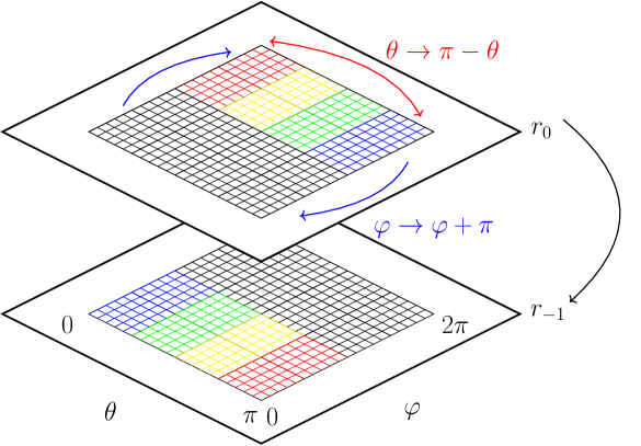
Figure 1: Diagram depicting the slab transfers involved in the $r_{\rm min}$ boundary condition.

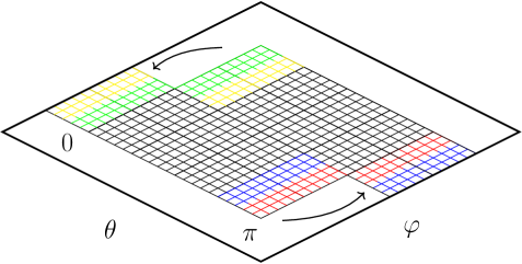
Figure 2: Diagram showing the slab transfers involved in the $\theta_{\min}$ and $\theta_{\rm max}$ boundary conditions.

The source slab for the boundary condition at the origin contains the first $n_{\rm gzr}$ physical points in $r$, where, again, $n_{\rm gzr}$ is the number of ghost zones in the $r$ direction, and all physical points in $\theta$ and $\varphi$. The operation $\theta\to\pi-\theta$ is performed by inverting the slab in the $\theta$ direction, while the $\varphi\to\varphi+\pi$ operation corresponds to moving all points from $[0,\pi]\to[\pi,2\pi]$ and, taking into account the periodicity in $\varphi$, all points from $[\pi,2\pi]\to[0,\pi]$. The $\varphi$ part of the operation is achieved using two separate calls to the slab transfer. Finally, the source slab is inverted in $r$ and the resulting slabs transferred into the ghost zones of the domain. This is illustrated in Fig. 1. Note that the procedure only fills ghost zones that correspond to physical points in $\theta$ and $\varphi$, while “double” and “triple” ghost zones on the edges and corners of the computational grid need to be filled by subsequent internal boundary conditions.

We then proceed by imposing the $\theta$ boundary conditions in a similar manner (see schematic in Fig. 2), followed by applying periodic boundary conditions in $\varphi$ using an existing thorn in the Einstein Toolkit. This order ensures that all ghost zones that need to be specified by internal parity boundaries are filled correctly.

In future applications that include magnetohydrodynamics and/or other matter fields, the same parity boundary conditions will apply to the matter fields as well. We have therefore implemented these boundary conditions in a separate thorn, SphericalBC, so that they are available for all evolved quantities, and not only for the spacetime evolution.

II.3 Time Step considerations

It is well known that the time integration of hyperbolic PDEs in spherical coordinates suffers from severe CFL time step restrictions, as the cell sizes become smaller and smaller with increasing latitude from the equator towards the poles, and decreasing distance from the origin. In a spherical unigrid in flat spacetimes, the time step due to the CFL condition is given by Baumgarte et al. (2013):

$$dt=\mathcal{C}\,{\rm min}\left[dr,\frac{dr}{2}d\theta,\frac{dr}{2}\sin(\frac{d\theta}{2})d\varphi\right],$$ (25)

where the CFL factor $\mathcal{C}$ is chosen between 0 and 1. The time step is therefore limited by the azimuthal distance between cells at the origin and polar axis. Compared with Cartesian coordinates, where $dt\approx dx$ (when the same spatial resolution $dx$ is used in all three coordinates), the time step in spherical coordinates varies as $dt\approx dr\,d\theta\,d\varphi$. Thus high angular resolution will impose severe time step restrictions in spherical coordinates.

When using a high number of azimuthal cells, the CFL restriction might render the numerical integration computationally unfeasible. There are several approaches to mitigate this problem (for an introduction, see e.g. Boyd (2001)), from various multipatch approaches Ronchi et al. (1996); Gomez et al. (1997); Bishop et al. (1997); Zink et al. (2008); Fragile et al. (2009); Reisswig et al. (2013); Kageyama and Sato (2004); Wongwathanarat et al. (2010); Melson et al. (2015); Shiokawa et al. (2017) to reducing the number of azimuthal cells at high latitudes as mesh coarsening in the azimuthal direction Liska et al. (2018), focusing resolution of the polar angle at the equator Korobkin et al. (2011); Noble et al. (2012), or the use of filters Shapiro (1970); Gent and Cane (1989); Jablonowski (2004); Müller (2015), to name a few.

To circumvent the severe time step limitation in cases when evolving BHs centered at the coordinate origin, we have devised a simple excision strategy in order to enlarge time steps in these evolutions. Specifically, we employ a radial extrapolation of all evolved variables deep inside the AH during the evolution, which essentially amounts to excising parts of the BH interior. Similar strategies have been employed and shown to work in the context of puncture BH Etienne et al. (2007); Brown et al. (2007, 2009). Within a fixed number of radial points the BSSN variables are not evolved but rather linearly extrapolated inwards radially from the first evolved points. When using this technique, we get a dramatic increase in time step, which is now given by:

$$dt=\mathcal{C}\,{\rm min}\left[dr,Adrd\theta,Adr\sin(\frac{d\theta}{2})d\varphi\right],$$ (26)

where $A\equiv n_{\rm Ex}-1+\frac{1}{2}$ and $n_{\rm Ex}$ is the number of “excised” radial grid points. In the simulations presented in Sec. III below, we choose this parameter such that $n_{\rm Ex}dr\approx r_{\rm AH}/2$ initially, and a CFL factor $\mathcal{C}=0.4$. We emphasize that we employ this excision for the purposes of speeding up the simulation only – it is not needed for stability. In Fig. 5 below we compare simulations with and without this excision; we also note that the simulations in Baumgarte et al. (2013, 2015); Baumgarte and Montero (2015); Baumgarte and Gundlach (2016); Gundlach and Baumgarte (2016, 2017); Ruchlin et al. (2018) did not use such an excision.

II.4 Diagnostics

We use the AHFinderDirect thorn Thornburg (2004); Schnetter et al. (2005) to find AHs Thornburg (2007) and the QuasiLocalMeasures thorn Dreyer et al. (2003); Schnetter et al. (2006) to calculate the angular momentum of the apparent horizon during the evolution. The BH spin is measured using the flat space rotational Killing vector method Campanelli et al. (2007) that was shown to be equivalent to the Komar angular momentum Komar (1959) in foliations adapted to the axisymmetry of the spacetime Mewes et al. (2015). Both thorns were written explicitly for the Cartesian coordinates employed in Carpet — interpolating entirely in the Cartesian basis both the ADMBase variables $\{\gamma_{ij},K_{ij},\alpha,\beta^{i}\}$ and the partial derivatives of the spatial metric and extrinsic curvature. As indicated in Sec. II.1 above, the ADMBase variables in the SphericalBSSN thorn are the physical metric, extrinsic curvature, lapse and shift in spherical coordinates, which means we need to transform the ADMBase variables and their partial derivatives to Cartesian coordinates after interpolation. This is required because AHFinderDirect expects the computational domain to have Cartesian topology (i.e., any surface with constant $r$, will not appear to be closed to AHFinderDirect). In its original form, AHFinderDirect interacts with the rest of the Toolkit by requesting the interpolation of the metric functions, and their derivatives, at various points in Cartesian coordinates. To make this work with SphericalBSSN, we modify this behavior by transforming the Cartesian coordinates to spherical (the necessary Jacobians are provided by aliased functions defined in SphericalBSSN), and then after the interpolation step, transforming the metric functions from spherical to Cartesian coordinates using the Jacobian $J^{a}{}_{i}\equiv\frac{\partial x^{a}}{\partial x^{i}}$ from spherical to Cartesian coordinates according to

$$\gamma_{ij} = J^{a}{}_{i}\,J^{b}{}_{j}\,\gamma_{ab},$$

$$\gamma_{ij,k} = J^{a}{}_{i,c}\,J^{b}{}_{j}\,J^{c}{}_{k}\,\gamma_{ab},$$

$$+ J^{a}{}_{i}\,J^{b}{}_{j,c}\,J^{c}{}_{k}\,\gamma_{ab},$$

$$+ J^{a}{}_{i}\,J^{b}{}_{j}\,J^{c}{}_{k}\,\gamma_{ab,c},$$

$$K_{ij} = J^{a}{}_{i}\,J^{b}{}_{j}\,K_{ab},$$

$$K_{ij,k} = J^{a}{}_{i,c}\,J^{b}{}_{j}\,J^{c}{}_{k}\,K_{ab},$$

$$+ J^{a}{}_{i}\,J^{b}{}_{j,c}\,J^{c}{}_{k}\,K_{ab},$$

$$+ J^{a}{}_{i}\,J^{b}{}_{j}\,J^{c}{}_{k}\,K_{ab,c},$$

$$\beta^{i} = J^{i}{}_{a}\,\beta^{a},$$ (27)

where we adopt the convention that indices $a$ and $b$ refer to spherical coordinates $r$, $\theta$ and $\varphi$, and indices $i$ and $j$ to the Cartesian coordinates $x$, $y$ and $z$ in coordinate transformations, and a comma indicates ordinary partial differentiation. When the origin of the AHFinderDirect internal six-patch system coincides with the coordinate origin, we add a small offset in $\theta$ at points located on the $z$-axis, as the Jacobian diverges at those points.

We extract GWs by computing the Weyl scalar $\Psi_{4}$ using the electric and magnetic parts of the Weyl tensor and constructing the numerical tetrad as described in Baker et al. (2002) in spherical coordinates. The calculation of $\Psi_{4}$ and the remaining Weyl scalars is contained in a new thorn called SphericalWeylScal. The multipole expansion of the real and imaginary parts of $\Psi_{4}$ in spin-weighted spherical harmonics Thorne (1980) is performed on the spherical grid used in the evolution. SphericalWeylScal performs the multipole expansion after the calculation of the Weyl scalars.

While the Jacobian for spherical coordinates is simple to implement directly into the analysis thorns, we coded our modification to AHFinderDirect and QuasiLocalMeasures so that they call aliased functions. In this way, both codes can now work with arbitrary coordinate systems, as the calculation of the Jacobians, etc., are handled by auxiliary routines.

II.5 Initial Data

As a demonstration of our methods we show in Sec. III below an evolution of a spinning Bowen-York BH Bowen and York (1980), which describes a perturbed Kerr BH Kerr (1963).

Bowen-York data are conformally flat, so that $h_{ij}=0$ identically, as well as $\bar{\Lambda}^{i}=0$. The data are also maximally sliced, so that $K=0$. The momentum constraint can then be solved analytically for the conformally rescaled extrinsic curvature; for rotating Bowen-York BHs, the only non-vanishing component is the $r\varphi$ component. Given the analytical solution for this extrinsic curvature, the Hamiltonian constraint can then be solved numerically for the conformal factor $e^{\phi}$. The only non-vanishing component of the extrinsic curvature variables $a_{ij}$ defined in (8) is then

$$a_{r\varphi}=\frac{3e^{-6\phi}J\sin\theta}{r^{3}},$$ (28)

where $J$ is the magnitude of the BH’s angular momentum (see also exercise 3.11 in Baumgarte and Shapiro (2010)).

In order to allow for future applications with more general sets of initial data that may have been prepared in Cartesian coordinates, we do not implement the above results directly, but instead use the TwoPunctures thorn Ansorg et al. (2004) to set up the data. This thorn uses spectral methods to solve the Einstein constraints, and interpolates the Cartesian ADMBase variables onto the computational mesh used in the simulation. We have adapted the thorn to interpolate the Cartesian ADMBase variables onto the spherical grid points instead. Upon the completion of the interpolation, the metric $\gamma_{ij}$ and extrinsic curvature $K_{ij}$ are transformed from Cartesian to spherical coordinates as described in Section II.4 above. The evolved metric variables $h_{ij}$ are then computed from

$$h_{ij}=e^{-4\phi}{\gamma}_{ij}\,\odot\,\begin{pmatrix}1&1/r&1/(r\,{\rm sin}\theta)\\ 1/r&1/r^{2}&1/(r^{2}\,{\rm sin}\theta)\\ 1/(r\,{\rm sin}\theta)&1/(r^{2}\,{\rm sin}\theta)&1/(r^{2}\,{\rm sin}^{2}\theta)\end{pmatrix}-\mathbbm{1},$$ (29)

where $\odot$ indicates the Hadamard product (element-wise matrix multiplication) and $\mathbbm{1}$ the identity matrix, while the evolved extrinsic curvature variables $a_{ij}$ are

$$\begin{split}a_{ij}=&e^{-4\phi}(K_{ij}-\frac{1}{3}{\gamma}_{ij}K)\\ &\odot\,\begin{pmatrix}1&1/r&1/(r\,{\rm sin}\theta)\\ 1/r&1/r^{2}&1/(r^{2}\,{\rm sin}\theta)\\ 1/(r\,{\rm sin}\theta)&1/(r^{2}\,{\rm sin}\theta)&1/(r^{2}\,{\rm sin}^{2}\theta)\end{pmatrix}.\end{split}$$ (30)

We confirmed that these variables agree with the values listed above to within truncation error.

We complete the specification of the initial data with choices for the initial lapse and shift. We choose an initial shift $\beta^{i}=0$ and an initial lapse $\alpha=e^{-2\phi}$ for the SphericalBSSN runs and $\beta^{i}=0$, $\alpha=2r/(M+2r)$ for the comparison Einstein Toolkit runs.

III Results

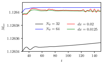
Figure 3: Comparison of the evolution of the irreducible mass of the BH for SphericalBSSN and McLachlan at two different resolutions each.

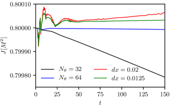
Figure 4: Comparison of the evolution of the AH angular momentum for SphericalBSSN and McLachlan at two different resolutions each.

	SphericalBSSN	McLachlan
Resolution	$dr=0.02$, $d\theta=\pi/32~{}(\pi/64)$, $d\varphi=2\pi/4$	$dx=dy=dz=0.02~{}(0.0125)$
Mesh refinement	unigrid	10 refinement levels Car
Outer boundary	200 (500)	512
Outer boundary condition	Sommerfeld BC Alcubierre et al. (2000)	Sommerfeld BC
FD order	4th order centered finite differencing	4th order centered finite differencing
Upwinding	4th order upwinding on shift advection terms	4th order upwinding on shift advection terms
Kreiss-Oliger dissipation	5th order dissipation	5th order dissipation
Dissipation strength	$\epsilon=0.1$	$\epsilon=0.1$
Time integration	Method of lines with RK4	Method of lines with RK4
CFL factor $\mathcal{C}$	0.4	0.4
Prolongation	none	5th order spatial, 2nd order temporal prolongation
Lapse evolution	1+log slicing Bona et al. (1995)	1+log slicing
Lapse advection	yes	yes
Shift evolution	$\Gamma$-driver Alcubierre et al. (2003), $\eta=1.0$	$\Gamma$-driver, $\eta=2.0$
Shift advection	yes	yes
Evolved conformal factor	$W=e^{-2\phi}$  Marronetti et al. (2008)	$W=e^{-2\phi}$
Gravitational wave extraction	$\Psi_{4}$ with SphericalWeylScal	$\Psi_{4}$ with WeylScal4 thorn Hinder et al. (2011)
GW extraction radii	20, 60, 100, 140, 180	20, 60, 100, 140, 180

Table 2: Summarizing the main parameters of the simulations performed with SphericalBSSN and the McLachlan thorn.

We perform simulations of a single, spinning, and initially conformally flat BH (the Bowen-York solution Bowen and York (1980)), with the initial data prepared as described in Section II.5 above. Since the Kerr Kerr (1963) spacetime is not conformally flat, these initial data represent a spinning BH with gravitational wave content that will be radiated away Gleiser et al. (1998), allowing the BH to settle to the Kerr solution. In all results presented here, dimensionful quantities are reported in terms of $M=1$. The BH has an initial spin $J=0.8M^{2}$ and an ADM mass Arnowitt et al. (1962, 2008) of $M_{\rm BH}=1.18112M$, giving a Kerr parameter $a\equiv J/M_{\rm BH}=0.677M$. We perform simulations of these initial data using our SphericalBSSN implementation. For comparison, we evolve the same initial data in Cartesian coordinates using the McLachlan Brown et al. (2009); Reisswig et al. (2011) thorn. McLachlan is a finite difference code generated using Kranc Husa et al. (2006) that solves the BSSN equations as part of the Einstein Toolkit. For our comparisons here we use 4th-order spatial finite differences in both codes, but we note that SENR/NRPy+ and McLachlan are capable of providing finite-difference stencils for the BSSN equations at arbitrary order. We summarize the details of the relevant simulation parameters in Table 2.

III.1 BH mass and spin

In Figs. 3 and 4 we plot the evolution of the irreducible mass of the BH and its angular momentum, respectively. During the first $35M$ of the evolution the BH mass increases due to the absorption of some of the GW content in the spacetime (see Fig. 5 below). We omit this initial time in Fig. 3, and instead show the long-term behavior after the BH has settled down. We show results for two different $\theta$ resolutions ($N_{\theta}=32$ and $64$) with SphericalBSSN and two resolutions ($dx=0.0125$ and $0.02$ on the finest mesh) using the Einstein Toolkit in Cartesian coordinates with box-in-box mesh refinement. The radial resolution in both evolutions ($dr=0.02$ and $dx=0.02$ on the finest Cartesian mesh which covers the AH) gives approximately 25 radial points across the minimum diameter (0.25) of the AH initially. For the irreducible mass shown in Fig. 3, the results obtained with the higher resolution SphericalBSSN and the two Cartesian runs agree well, while the lower resolution SphericalBSSN run appears to be under-resolved, showing a linear growth in the irreducible mass that is unphysical. There is a notable absence of oscillations in the higher resolution SphericalBSSN run, which can be seen in both Cartesian runs (converging away with increasing resolution).

The evolution of the angular momentum of the AH, shown in Fig. 4, exhibits a similar behavior. The two high-resolution runs with McLachlan and SphericalBSSN perform similarly, while the lower resolution runs show linear drifts in both Cartesian and spherical coordinates. The Cartesian simulations show larger initial oscillations that do not seem to converge away with increasing resolution, likely due to reflections of short-wavelength modes across mesh boundaries Zlochower et al. (2012); Etienne et al. (2014). Just as for the irreducible mass, the high-resolution SphericalBSSN simulations performs best.

To test the effect of the excision described in Section II.3, we plot the initial evolution of the irreducible mass for a run with, and one without, our excision procedure in Fig. 5. Evidently, the excision procedure does not have any visible effect on the accuracy or stability of our method.

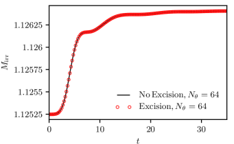
Figure 5: Comparing the evolution of the BH irreducible mass for two SphericalBSSN runs, with and without the excision algorithm described in Sec. II.3.

III.2 Gravitational waves

In Fig. 6, we plot the absolute value of the multipole expansion in spin-weighted spherical harmonics ${}_{-2}Y_{lm}$ of the Weyl scalar $\Psi_{4}$, extracted at a radius of $r=180$, for the even $l=2$ through 8, $m=0$ multipoles (by symmetry, only the $m=0$ modes are non-zero). The plot shows the Cartesian simulation with $dx=0.02$ and two different $\theta$-resolutions for the spherical simulations. There are notable differences between the Cartesian and spherical evolutions: In the spherical simulations, there is an absence of initial noise pulse before the radiation reaches it peak value, and the decay after the peak value proceeds much cleaner and to orders of magnitude below the values attained in the Cartesian simulation. The reason for this difference in behavior is the fact that there are partial reflections of the outgoing wave at each Cartesian mesh refinement boundary (see, e.g. Zlochower et al. (2012); Etienne et al. (2014)), causing the unphysical excitation of $l\geq 4$ multipole modes, as well as reflections in the initial noise pulse in seen in the $l=2$ mode. These reflections affect strong-field quantities as well, as described in Etienne et al. (2014). Contrary to this, the spherical grid in SphericalBSSN is a single uniform grid, so there is a complete absence of these reflections (apart from reflections from the outer boundary), leading to much cleaner signals especially in the higher-order multipoles.

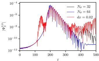
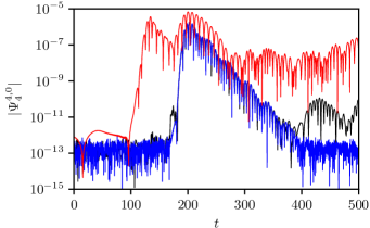
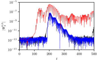
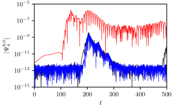
Figure 6: $|\Psi_{4}|$ for the even $l=2$ through 8, $m=0$ modes, computed with both SphericalBSSN (black and blue lines) and McLachlan (red lines).

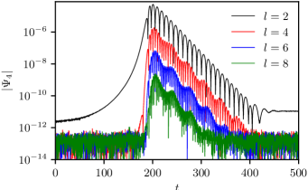
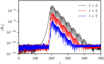
Figure 7: $|\Psi_{4}|$ for the even $l=2$ through 8, $m=0$ modes (left panel), and the odd $l=3$ through 7, $m=0$ modes (right panel), computed with SphericalBSSN.

III.3 Kerr quasinormal modes

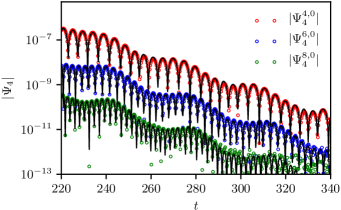
Figure 8: Fits for the QNM ringdown, with even modes $l=2$ through $8$ in the left panel, and odd modes $l=3$ through 7 in the right panel. The solid lines represent the numerical results for $|\Psi_{4}|$ as as computed with SphericalBSSN, while the points are a result of a fit (33) to these numerical data.

Given that the SphericalBSSN simulation provides us with very accurate higher order modes, we turn our attention to an analysis of the BH’s quasinormal modes. As explained in the setup of the initial data, the spinning, initially conformally flat BH should settle down to a Kerr BH via ringdown of its quasinormal modes (QNM) (see Berti et al. (2009) for a review). In Fig. 7, we plot the $l=2$ through 8, $m=0$ modes of $|\Psi_{4}|$ for the high resolution $N_{\theta}=64$ simulation alone. We note that even (odd) $l$-modes contain only the real (imaginary) part of $\Psi_{4}$. The $l=2$ mode follows a clear exponential decay, but the higher-order modes exhibit a beating modulation on top of the exponential decay. The reason for this behavior is that the quasinormal modes for Kerr are defined in terms of spheroidal harmonics, ${}_{s}{S}_{lm}$, while we decompose the waveform in terms of spin-weighted spherical harmonics ${}_{s}Y_{lm}$. Following Teukolsky (1972), we can decompose $\Psi_{4}$ in terms of spin-weighted spheroidal harmonics ${}_{s}S_{l^{\prime}m}$ with $s=-2$ according to

$$\Psi_{4}=\sum_{l^{\prime},m^{\prime},n^{\prime}}A_{l^{\prime}m^{\prime}n^{\prime}}\,{}_{s}S_{l^{\prime}m^{\prime}}e^{-\alpha_{l^{\prime}m^{\prime}n^{\prime}}t}e^{i\omega_{l^{\prime}m^{\prime}n^{\prime}}t}$$ (31)

where $n$ is the overtone number of each mode, $\alpha_{l^{\prime}mn}$ is its the decay rate, $\omega_{l^{\prime}mn}$ its frequency, and the coefficients $A_{l^{\prime}mn}$ are the amplitudes of the individual modes. In particular, we see that each mode oscillates and decays at well-defined rates. In practice, however, $\Psi_{4}$ is projected into the spin-weighted spherical harmonics ${}_{s}Y_{lm}$, i.e.

$$\Psi_{4}^{lm} = \int\Psi_{4}{}_{s}Y^{*}_{lm}d\Omega$$ (32)

$$= \sum_{l^{\prime},m^{\prime},n^{\prime}}A_{l^{\prime}m^{\prime}n^{\prime}}e^{-\alpha_{l^{\prime}m^{\prime}n^{\prime}}t}e^{i\omega_{l^{\prime}m^{\prime}n^{\prime}}t}\int{}_{s}S_{l^{\prime}m^{\prime}}{}_{s}Y^{*}_{lm}d\Omega$$

$$= \sum_{l^{\prime},m^{\prime},n^{\prime}}A_{l^{\prime}m^{\prime}n^{\prime}}e^{-\alpha_{l^{\prime}m^{\prime}n^{\prime}}t}e^{i\omega_{l^{\prime}m^{\prime}n^{\prime}}t}\mu^{*}_{mll^{\prime}n^{\prime}}(a)\delta_{mm^{\prime}}$$

$$= \sum_{l^{\prime},n^{\prime}}A_{l^{\prime}mn^{\prime}}e^{-\alpha_{l^{\prime}mn^{\prime}}t}e^{i\omega_{l^{\prime}mn^{\prime}}t}\mu^{*}_{mll^{\prime}n^{\prime}}(a).$$

Here the coefficients $\mu^{*}_{mll^{\prime}n^{\prime}}(a)$ describe the mixing between spin-weighted spheroidal and spherical harmonics; they are defined in eq. (5) of Berti and Klein (2014) and depend on the black hole Kerr parameter $a$.

Ignoring higher-order overtone modes with $n^{\prime}>0$, which decay faster than the fundamental modes, we fit the $l=3$ through 8, $m=0$ spherical harmonic modes computed from our numerical data to the form

$$\Psi^{l0}_{4}(t)\approx~{}\sum_{l^{\prime}=2}^{l^{\prime}=10}A_{l^{\prime}0}e^{(-\alpha_{l^{\prime}00}t)}{\rm sin}(\omega_{l^{\prime}00}t+\phi_{l^{\prime}0}),$$ (33)

where the unknowns $A_{l^{\prime}0}$ and $\phi_{l^{\prime}0}$ serve as 18 parameters corresponding to the amplitudes (including the mixing coefficients) and phases, respectively. We fix the $\alpha_{l^{\prime}00}$ and $\omega_{l^{\prime}00}$ in the fit to be the values of the decay rate and frequency that correspond to the Kerr BH in our simulation ($J/M_{\rm BH}^{2}=0.573$ and $M_{\rm BH}=1.18112$), using the tabulated values and Mathematica notebooks to calculate QNMs Berti et al. (2006, 2009) found at Ber . The results of the fit for the $l=3$ through 8 modes are shown in Fig. 8 for a fitting window of $t=220-340$. The beating of the modes is very well captured by modeling a given $l$ mode as the sum of the expected decay rates and frequencies calculated in spin-weighted spheroidal harmonics, showing that mode mixing is responsible for the observed beating. A similar type of equal $m$ mode mixing has been observed in Kelly and Baker (2013).

IV Discussion

We report on an implementation of the BSSN equations in spherical coordinates in the Einstein Toolkit. While Cartesian coordinates have advantages for many applications, spherical coordinates are much better suited to take advantage of the approximate symmetries in many astrophysical systems. The problems associated with the coordinate singularities that appear in curvilinear coordinates can be avoided if these singularities are treated analytically – which, in turn, is possible with the help of a reference-metric formulation of the BSSN equations Bonazzola et al. (2004); Shibata et al. (2004); Brown (2009); Gourgoulhon (2012); Montero and Cordero-Carrión (2012) and a proper rescaling of all tensorial quantities Montero and Cordero-Carrión (2012); Baumgarte et al. (2013, 2015); Ruchlin et al. (2018). We implement this formalism in the Einstein Toolkit in an effort to make these techniques publicly available to the entire numerical relativity community and beyond.

Specifically, we adapt the Einstein Toolkit infrastructure, which originally was designed for Cartesian coordinates, for spherical coordinates. In contrast to Cartesian coordinates, spherical coordinates feature inner boundary condition, where ghost zones are filled by copying interior data from other parts of the numerical grid, taking into account proper parity conditions. We implemented these boundary conditions, which may require communication across processors, within an MPI-parallelized infrastructure using the Slab thorn. Numerical code for the BSSN equations in spherical coordinates were provided by SENR/NRPy+ Ruchlin et al. (2018); SEN .

In order to test and calibrate our implementation we performed simulations of a single, spinning and initially conformally flat BH, and compared the evolution of BH mass, spin and GWs using our spherical BSSN (SphericalBSSN) and Cartesian AMR BSSN (McLachlan) code with comparable grid resolutions. For sufficiently high resolutions, the evolution on a spherical mesh conserves irreducible mass and angular momentum far better than with Cartesian AMR. In particular, there are no reflections of the initial junk radiation or outgoing initial gauge pulse Etienne et al. (2014); Zlochower et al. (2012) at mesh refinement boundaries, causing the evolution of irreducible mass and spin to be smoother in the unigrid spherical evolution. The advantage of using unigrid spherical coordinates over Cartesian coordinates with box-in-box mesh refinement becomes particularly apparent when analyzing the higher-order $l$-multipoles of the GW wave signal. These signals are affected by partial reflections at mesh refinement boundaries, leading to a contamination of all higher order $l,m$ modes that never fully leaves the computational domain. This effect is completely absent in the simulations using the SphericalBSSN thorn, where the quasinormal ringdown of the Kerr BH is observed to much smaller amplitudes than in the Cartesian simulations. We observe a significant beating of the exponential ringdown of multipoles with $l>2$, which can be explained by spheroidal-spherical multipole mode mixing. The accurate modeling of the ringdown of higher order modes is necessary in order to provide GW detectors with accurate templates Berti et al. (2007), as the measurement of two quasinormal modes is needed to test the “no hair theorem” Dreyer et al. (2004); Berti et al. (2006).

The current SphericalBSSN thorn adopts uniform resolution in radius, which requires a large number of points in order to place the outer boundary sufficiently far away and to avoid contaminating the inner parts of the computational domain with noise from the outer boundary (i.e., to causally disconnect these inner parts from the outer boundary). Possible approaches to improve this is to adopt a non-uniform radial grid, e.g. a logarithmic grid as implemented in Baumgarte and Montero (2015) or Sanchis-Gual et al. (2015), or to use more general radial coordinates. The SENR/NRPy+ code Ruchlin et al. (2018); SEN allows for such generalized radial coordinates – a convenient choice is $\sinh(r)$ – and we plan to port these features into the SphericalBSSN thorn in the future.

We also plan to supplement our current implementation of Einstein’s vacuum equations in spherical coordinates with methods for relativistic hydrodynamics and magnetohydrodynamics as another set of publicly available thorns for the Einstein Toolkit. As shown in Montero et al. (2014); Baumgarte et al. (2015), these equations can be expressed with the help of a reference-metric as well. Further using a rescaling of all tensorial quantities similar to the rescaling of the gravitational field quantities in this paper, the evolution of hydrodynamical variables is unaffected by the coordinate singularities. We hope that with these methods, and possibly implementations of microphysical processes like radiation transport and nuclear reaction chains, the Einstein Toolkit in spherical coordinates will become a powerful and efficient community tool for fully relativistic simulations of a number of different objects, including rotating neutron stars, gravitational collapse, accretion disks, and supernova explosions. We believe that this will result in a new open source state-of-the-art code that will prove to be a valuable resource for a broad range of future simulations.