Fluid-supported elastic sheet under compression: Multifold solutions

Abstract

The properties of a hinged floating elastic sheet of finite length under compression are considered. Numerical continuation is used to compute spatially localized buckled states with many spatially localized folds. Both symmetric and antisymmetric states are computed and the corresponding bifurcation diagrams determined. Weakly nonlinear analysis is used to analyze the transition from periodic wrinkles to single fold and multifold states and to compute their energy. States with the same number of folds have energies that barely differ from each other and the energy gap decreases exponentially as localization increases. The stability properties of the different competing states are established and provide a basis for the study of fold interactions.

I Introduction

Recent experiments (Pocivavsek et al., 2008) have shown that an elastic sheet on the surface of a liquid undergoes a series of transitions when compressed in the longitudinal direction: for small compression the sheet deforms into a periodic array of wrinkles; with increasing compression the deformation of the sheet becomes more and more nonlinear and the deformation spontaneously localizes. This process continues until the sheet makes contact with itself.

These experiments have stimulated several efforts at modeling this sequence of transitions (Diamant and Witten, 2011; Audoly, 2011; Rivetti and Neukirch, 2014; Oshri et al., 2015). The equilibrium configurations are described by a fourth-order equation for the deformation angle as a function of arclength. This equation, as well as others describing post-buckling phenomena of elastic media under compression (Hunt et al., 2000) and torsion (Thompson and Champneys, 1996; Champneys and Thompson, 1996), is of Swift-Hohenberg type and its solutions bear a number of similarities to existing analysis of steady states of the Swift-Hohenberg equation with a quadratic nonlinearity (Champneys and Groves, 1997), or equivalently to the small amplitude behavior of the quadratic-cubic Swift-Hohenberg equation (SH23) as described, for instance, in Refs. (Burke and Knobloch, 2006; Knobloch, 2015). Specifically, on an infinite domain one expects that the primary instability to the wrinkled state is accompanied by the simultaneous appearance of two branches of spatially localized solutions, one characterized by deformation that peaks in the center of the domain and the other that dips in the center. The theory tells us that on an infinite domain these states are described by the normal form for the reversible Hopf bifurcation (in space) with 1:1 spatial resonance (Iooss and Pérouème, 1993). In particular, the branches of localized solutions are initially exponentially close to one another (Kozyreff and Chapman, 2006; Chapman and Kozyreff, 2009; Gaivão and Gelfreich, 2011), but gradually separate as the compression of the sheet increases and the solutions begin to localize.

Of course, in the experiments the sheet is of finite length. In this case existing theory shows that the 1:1 reversible Hopf bifurcation breaks apart into a primary bifurcation to a wrinkled state followed, at small amplitude, by a secondary bifurcation that creates a pair of spatially modulated wrinkled states, one with maxima in the center and the other with minima in the center. This bifurcation is an example of an Eckhaus instability of the periodic wrinkled state and its dependence on the domain length has been studied in detail (Bergeon et al., 2008). In particular, it is known that subsequent secondary bifurcations lead to the so-called multipulse states, i.e., states with more than one localized structure within the available domain (Burke and Knobloch, 2009). However, since the periodically wrinkled state does not exhibit a saddle-node bifurcation the correspondence with SH23 does not extend to larger amplitude states; in particular, homoclinic snaking (Burke and Knobloch, 2006; Knobloch, 2015) is absent.

In this paper we use the similarity between the present problem and the Swift-Hohenberg equation to identify new classes of localized wrinkled structures on finite domains (Peletier and Troy, 2006). We focus on the case of a thin elastic sheet allowing us to neglect its contribution to the gravitational potential energy when its is deformed. In this case the model equation is odd in the dependent variable, a symmetry respected by the hinged boundary conditions we employ. As a consequence the system admits four types of localized states instead of the two mentioned above. two even parity states under spatial reflection and two odd parity states. Of these the even states correspond to deformation that either peaks or dips in the center of the domain while the odd parity states consist of symmetry-related peak-trough combinations. Consequently the system exhibits four branches of spatially localized states, and so its properties in fact resemble more closely those of the small amplitude states in the cubic-quintic Swift-Hohenberg equation (Burke and Knobloch, 2007a, b) rather than those of the quadratic-cubic Swift-Hohenberg equation.

Each of these solutions is a single fold solution, with a fold either in the center of the sheet or split between the two end points. However, the problem also admits a vast array of multifold states consisting of both identical and nonidentical folds at different locations along the sheet. We compute here both single fold and multifold states using numerical continuation techniques that have proved invaluable in the studies of the Swift-Hohenberg equation, as well as weakly nonlinear theory of the type first employed in the present context in (Oshri et al., 2015) and discuss the stability properties of these distinct states.

The paper is organized as follows. In the following subsection we summarize the basic properties of the model we use. We then focus on finite sheets, and discuss in turn periodic structures in sheets with hinged ends and the wrinkle-to-fold transition. The word ’fold’ is here employed to mean a strongly spatially localized deformation. We compute fold solutions with both positive and negative deformation in the center, as well as multifold structures. We also compute the free energy of these structures, and identify structures corresponding to minima of the free energy with the stable states observed in experiments. Our results can be considered to be an extension of the work of Diamant and Witten (2011); Rivetti (2013) to finite domains and extend the analysis in Oshri et al. (2015); Marple et al. (2015) to multifold states.

I.1 Governing equations

Consider an elastic sheet of length $L$ and bending modulus $B$ lying on a semi-infinite fluid substrate of density $\rho$. In static equilibrium under gravity, a compression $\Delta$ in the $x$ direction will deform the sheet in the $y$ direction as shown in Fig. 1. The shape of the sheet can be parametrized in terms of the arclength $s$ and the local angle $\phi(s)$ between the sheet and the horizontal axis. Cartesian coordinates $\left[x(s),y(s)\right]$ are related to this parametrization through $x(s)=\int_{-\frac{L}{2}}^{s}\cos\phi(s)\,\mbox{d}s,\text{\quad}y(s)=\int_{-\frac{L}{2}}^{s}\sin\phi(s)\,\mbox{d}s.$ Accordingly, the total energy stored (per unit of length in the $z$ direction) due to the deformation is

$$E\left[\phi\right]=\int_{-L/2}^{+L/2}\mbox{d}s\,\left(\frac{1}{2}B\dot{\phi}^{2}+\frac{1}{2}\rho gy^{2}\cos\phi\right),$$ (1)

where the dot denotes derivative with respect to $s$ and $g$ is the acceleration due to gravity. The first term is the bending energy while the second represents the gravitational potential energy of the deformed state. The sheet shape is linked to the total compression through

$$\Delta\left[\phi\right]=\int_{-L/2}^{+L/2}\mbox{d}s\,\left(1-\cos\phi\right).$$ (2)

Thus the load $P$ required to keep the system in equilibrium is equal to $dE/d\Delta$.

The natural lengthscale of the system, $\lambda=\left[B/(\rho g)\right]^{1/4}$, can be used to nondimensionalize the quantities $x,y,s,\Delta$ and $L$. Likewise, the energy $E$ can be scaled by $B/\lambda$ and $P$ by $B/\lambda^{2}$. This rescaling leads to a simpler version of Eq. (1) with $B=\rho g=1$.

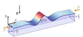
Figure 1: (Color online) Schematic view of the formation of a wrinkled pattern on an elastic sheet over a fluid substrate under compression. The shape of the sheet can be parametrized in terms of the local angle $\phi(s)$ that the sheet forms with the horizontal. The parameter $s$ represents the arclength along the sheet, whose total length $L$ is fixed.

We study quasistatic deformations of an elastic sheet under the following two conditions: (i) a fixed load $P$ (dead loading), or (ii) fixed compression $\Delta$ (rigid loading). An equation for the shape of the sheet, $\phi(s)$, can be derived in both cases using a Lagrangian approach as shown in (Audoly, 2011; Diamant and Witten, 2011). Whether minimizing the functional $E[\phi]$, the energy, for given $\Delta$ (rigid loading) or, equivalently, minimizing the functional $G\left[\phi\right]\equiv E-P\Delta$, the free energy, for given $P$ (dead loading), one finds that $\phi(s)$ satisfies

$$\ddddot{\phi}+\frac{3}{2}\dot{\phi}^{2}\ddot{\phi}+p\ddot{\phi}+\sin\phi=0,$$ (3)

where $p$ depends on the boundary conditions. We adopt here hinged boundary conditions, i.e., the conditions $\left.y\right|_{\pm L/2}=\left.\ddot{y}\right|_{\pm L/2}=0$ (or, equivalently, $\left.\dot{\phi}\right|_{\pm L/2}=\left.\dddot{\phi}\right|_{\pm L/2}=0$), so $p$ is related to the static load $P$ by (Oshri et al., 2015)

$$P=p\cos\phi\left(\pm L/2\right)-\ddot{\phi}\left(\pm L/2\right)\sin\phi\left(\pm L/2\right).$$ (4)

With these boundary conditions the system is invariant under the transformations $\phi\rightarrow-\phi$ and $s\rightarrow-s$, which are linked to invariance with respect to $x\rightarrow-x$ and $y\rightarrow-y$.

Equation (3) conserves the following quantity along the sheet:

$$H\left[\phi\right]=\dddot{\phi}\mbox{$\dot{\phi}$}-\frac{1}{2}\ddot{\phi}^{2}+\frac{3}{8}\dot{\phi}^{4}+\frac{1}{2}p\dot{\phi}^{2}-\cos\phi.$$

For hinged sheets $H=\left.-\frac{1}{2}\ddot{\phi}^{2}\right|_{\pm L/2}-\cos\left.\phi\right|_{\pm L/2}$. Throughout this article both dead and rigid loading approaches will be considered and the results will therefore be represented either in terms of the quantities $\left(P,G\right)$ or $\left(\Delta,E\right)$, as appropriate. The difference between these two approaches is fundamental importance for the stability analysis as discussed in Sec. II.5.

I.2 Exact solutions for an infinite sheet

Despite the presence of nonlinear terms, Eq. (3) admits explicit solutions for the case of an infinite sheet. Two families of spatially localized solutions can be found (Diamant and Witten, 2011): a family of symmetric solutions,

$$\phi_{s}\left(s\right)=4\arctan\left[\frac{\kappa\sin k\left(s-s_{0}\right)}{k\cosh\kappa\left(s-s_{0}\right)}\right]$$ (5)

and a family of antisymmetric solutions:

$$\phi_{a}\left(s\right)=4\arctan\left[\frac{\kappa\text{$\cos$}k\left(s-s_{0}\right)}{k\cosh\kappa\left(s-s_{0}\right)}\right].$$ (6)

Here $s=s_{0}$ corresponds to the symmetry point while $k=\frac{1}{2}\sqrt{2+P}$ and $\kappa=\frac{1}{2}\sqrt{2-P}$, i.e., the solutions exist only for $P<2$. Evaluation in the limit $s\rightarrow\pm\infty$ shows that for this case $P=p$. The extra parameter $s_{0}$ is a result of the invariance of the infinite sheet under transformations of the form $s\rightarrow s+{\rm const}$. In the literature, localized solutions are referred to as folds. These solutions are members of a wider family of solutions, obtained by adding an extra phase to the trigonometric function, i.e.,

$$\phi_{f}\left(s\right)=4\arctan\left[\frac{\kappa\text{$\cos$}\left[k\left(s-s_{0}\right)-\varphi_{f}\right]}{k\cosh\kappa\left(s-s_{0}\right)}\right].$$ (7)

Thus the symmetric and antisymmetric solutions correspond to the particular cases $\varphi_{f}=\pi/2$ and $\varphi_{f}=0$, respectively. The asymmetric family ($\varphi_{f}\neq 0,\pi/2$) has been shown to describe the shape of an elastic sheet when extracted from a fluid bath (Rivetti, 2013).

On the other hand, periodic solutions on an infinite sheet can be found in terms of Jacobi elliptic functions,

$$\phi\left(s\right)=2\arcsin\left[k\,\mathrm{sn}_{k}\left(qs-\vartheta_{0}\right)\right],$$ (8)

or, equivalently,

$$y\left(s\right)=\frac{2k}{q}\,\mathrm{cn}_{k}\left(qs-\vartheta_{0}\right),$$ (9)

and exist for $0<k<1$. The quantity $q$ is related to $k$ and the static load $P$ by the implicit relation

$$P=q^{2}+\left(1-2k^{2}\right)q^{-2}.$$ (10)

Thus $q^{2}-q^{-2}<P<q^{2}+q^{-2}$. The solutions (8) have a period equal to $4K(k)/q$, where $K\left(k\right)$ is the complete elliptic integral of the first kind. Periodic solutions are usually referred to as wrinkles in the literature, cf. (Cerda and Mahadevan, 2003; Brau et al., 2013) and references therein.

I.3 Explicit periodic solutions for finite sheets

Exact periodic solutions of Eq. (3) for finite sheets can easily be found by matching properly both $\vartheta_{0}$ and the period of Eq. (8) with the boundary conditions. For hinged boundary conditions, it follows that

$$\vartheta_{0}=\nu_{n}K(k),\quad q_{n}=\frac{2nK(k)}{L},\quad n=1,2,3...,$$ (11)

where $\nu_{n}=1$ for $n$ odd and $\nu_{n}=0$ for $n$ even (see (Oshri et al., 2015) for details). As expected, the finiteness of the sheet discretizes the parameter $q$ into discrete families $q_{n}(k)$ labeled by the index $n$ (the number of half-periods of the solution). Solutions of this type will be referred to as $\phi_{n}$. Here $k$ quantifies the amplitude of the solution as measured, for example, by the mean compression per unit length $\overline{\Delta}\equiv\Delta/L$:

$$\overline{\Delta}=2I(k).$$ (12)

Here $I(k)\equiv 1-E(k)/K(k)$ and $E(k)$ is the complete elliptic integral of the second kind. Remarkably, this expression does not depend on $n$.

The mean energy per unit length, $\overline{E}\equiv E/L$, is given by

$$\overline{E}=2\left(q_{n}^{2}+q_{n}^{-2}\right)\left[k^{2}-I(k)\right]-\left[a_{k}-b_{k}I(k)\right],$$ (13)

where $a_{k}=8q^{-2}\left(k^{4}+k^{2}\right)/15$ and $b_{k}=16q^{-2}\left(k^{4}-k^{2}+1\right)/15.$ The mean free energy $\overline{G}=\overline{E}-P\overline{\Delta}$ now follows from Eqs. (12)–(13). For a given $n$ and $L$, Eqs. (10)–(13) determine $\left(P,\overline{\Delta},\overline{E},\overline{G}\right)$ in terms of the single continuous parameter $k$. Figure 2 depicts the resulting solution branches in the $\left(\overline{\Delta},\overline{E}\right)$ plane for $L=20\pi$ and different $n$ values.

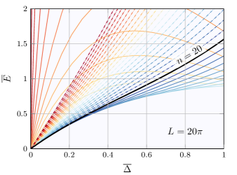
Figure 2: (Color online) Branches of periodic states $\phi_{n}$ in the $(\overline{\Delta},\overline{E})$ plane for a sheet of fixed length $L=20\pi$. Each curve corresponds to a different family $q_{n}(k)$, $n=1,2,...,40$, with $k$ related to $\overline{\Delta}$ by Eq. (12). The branch for $n=20$ has the least energy near the common bifurcation point at the origin. Dash-dotted branches correspond to $n>20$.

Periodic solutions for finite sheets bifurcate from the trivial state $\phi(s)=0$ at $k=0$. Since $E(0)=K(0)=\pi/2$, each periodic branch $\phi_{n}$ bifurcates from the $P$-axis at

$$P_{n}^{*}=q_{n}^{2}+q_{n}^{-2}$$ (14)

and $\Delta_{n}^{*}=0$. Thus $P_{n}^{*}\geq 2$ with equality at $n=L/\pi$. To determine which solution emerges spontaneously when the sheet is compressed, we expand Eqs. (12) and (13) around $k=0$, yielding $\overline{E}\approx\left(q^{2}+q^{-2}\right)k^{2}$ and $\overline{\Delta}\left(k\right)\approx k^{2}.$ It follows that $\overline{E}\approx\left(q^{2}+q^{-2}\right)\overline{\Delta}.$ The branch with minimal energy in the $\left(\overline{\Delta},\overline{E}\right)$ plane near the trivial state is that which minimizes the slope $q_{n}^{2}+q_{n}^{-2}\approx P_{n}^{*}$ of the energy. Hence, the branch bifurcating at the lowest $P_{n}^{*}$ value is the only one that is stable in the vicinity of the primary bifurcation.

The branches $\phi_{n}$ and $\phi_{n+1}$ bifurcate simultaneously from the trivial state whenever $L_{(n,n+1)}=\pi\sqrt{n(n+1)}$ and do so at $P_{(n,n+1)}^{*}=2+\left[n(n+1)\right]^{-1}$. These conditions define the range of $L$ for which the $n$th solution is stable: $L_{(n-1,n)}<L<L_{(n,n+1)}$. As $L\rightarrow\infty$, the width of this range converges to $\pi$ and its center to $\pi n$.

Far from the primary bifurcation, corresponding to $k=0$, other branches may display lower energies than the branch that minimizes $P_{n}^{*}$. This is illustrated in Fig. 2, which shows that the lower $n$ branches eventually cross the $n=20$ branch as $\overline{\Delta}$ increases.

II Folds in Finite Sheets

II.0.1 Numerical continuation of localized patterns

Since no explicit exact localized solutions of Eq. (3) exist for elastic sheets of finite length and hinged boundary conditions, we employ numerical continuation (Doedel et al., 1991a, b) to follow different solution types of this problem through parameter space. For this purpose, we implemented Eq. (3) in the AUTO${}^{\text{©}}$ code (Doedel et al., 2008) with hinged boundary conditions, with the independent variable $s$ transformed so the original half domain $\left[-L/2,0\right]$ becomes $\left[0,1\right]$. Since the quantities $\left(\overline{\Delta},\overline{E},\overline{G},P\right)$ are all functions of the parameters $\left(p,L\right)$ of the system, we plot the results as a function of $P$ instead of $p$, for fixed length $L=l\pi$ ($l\in\mathbb{R}$).

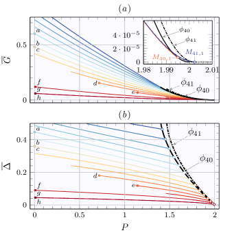
Figure 3: (Color online) Results from numerical continuation of Eq. (3) subject to hinged boundary conditions, showing different solution branches in the form (a) $\overline{G}(P)$ and (b) $\overline{\Delta}(P)$, both for $L=40\pi$. The thick black line represents the periodic state $n=40$, which undergoes several bifurcations as $P$ decreases (see text for details). The other branches represent multifold states. The solutions shown in Fig. 4 correspond to the labeled symbols $\blacksquare$ (b-c and g-h overlap). The inset in (a) shows the region near the origin where the symmetric and antisymmetric fold solutions first appear. Bifurcation points are marked as $\circ$. The $n=41$ periodic branch (dashed line) is also displayed. No discernible difference between the results of the analysis of Sec. II.1 (thin lines) and the numerical continuation results is seen.

Numerical continuation requires an initial guess. Taking advantage of the existence of explicit periodic solutions, we performed continuation on a $128$ point spatial grid starting from solutions (8) for a given $n$ and a high value of $k$, i.e., $\phi_{n}$ far from the trivial state. The code was tuned to detect bifurcation points along this branch as $P$ increases towards the onset value $P^{*}$. Figure 3(a-b) displays the branches $\phi_{40}$ and $\phi_{41}$ in black, both for $L=40\pi$. Each periodic branch displays a set of bifurcation points with decreasing separation as $P$ increases towards $P^{*}$. For $\phi_{40}$ these bifurcation points are shown Fig. 3(b). These bifurcation points will be referred to as $M_{n,m}$, where the integer $n$ specifies the primary periodic state and the integer $m$ counts the bifurcations from this state starting from the primary bifurcation $P_{n}^{*}$. Thus $M_{40,1}$ denotes the secondary bifurcation closest to $P_{40}^{*}$.

At each of the secondary bifurcation points $M_{n,m}$ we switched the branch direction and ran the numerical continuation for decreasing $P$ until $P=0$ was attained. The new branches are also displayed in Fig. 3 but now in color. Some of the solutions far from the bifurcation points $M_{n,m}$ are depicted in Fig. 4. A simple inspection [see inset in Fig. 3(a)] shows that the branch starting at $M_{40,1}$ corresponds to a localized antisymmetric fold while that starting at $M_{41,1}$ is a symmetric fold. The former bifurcation point is located quite far from $P_{40}^{*}$, i.e., at finite amplitude, while the latter lies very close to $P_{41}^{*}$. At this value the $\phi_{41}$ state barely departs from the trivial state. For $L=41\pi$ the situation is the opposite: the symmetric fold is the one that bifurcates at finite amplitude (from the $\phi_{41}$ branch), while the antisymmetric fold bifurcates at a very small amplitude (from the $\phi_{42}$ branch). In any case, the symmetric and antisymmetric branches approach each other very fast as they depart from their respective branch point with decreasing $P$.

Figure 4: (Color online) Antisymmetric solutions ($b$-$h$) from numerical continuation for different values of $m$ defined in the text and $n=40$ computed on a domain of length $L=40\pi$. The location of each solution in parameter space is indicated in Fig. 3. The solutions acquire additional folds as $m$ increases. The symmetric solution $\phi_{41,1}$ (a) bifurcates from the $n=41$ periodic state, and does so very close to the trivial state, as shown in the inset in Fig. 3(a). The periodic solutions $\phi_{40}$ and $\phi_{41}$ at high compression ($\overline{\Delta}=0.55$) are included for reference.

Solutions $\phi_{n,m}$ with $m>1$ represent $m$-fold solutions, i.e., arrays of $m$ equispaced folds. Examples are shown in Fig. 4. Although reported in Marple et al. (2015), these multifold solutions have not been described in detail. Multifold solutions $\phi_{n,m}$ for a fixed $l$ do not exist for arbitrary $n$ and $m$. For instance, for $l=40,$ one-fold solutions ($m=1$) are observed only for $n=40$ and $41$ while two-fold solutions ($m=2$) are only found for $n=39,40,41,42$. In general, $2m+2$ solutions with $m$ folds were detected for $n$ varying from $l-m+1$ to $l+m$.

II.1 Weakly modulated solutions

Multiscale analysis describes successfully several features of this system and, in particular, the wrinkle-to-fold transition (Brau et al., 2010; Audoly, 2011). Herein, we use this approach to understand the emergence of the solutions obtained in Sec. II.0.1. The system is assumed to be subject to hinged boundary conditions and finite. The domain of $s$ is mapped into $s\in\left[0,L\right]$ for the sake of simplicity in the application of the boundary conditions.

We seek multiscale solutions of Eq. (3) in the form

$$y\left(s\right)=\sum_{j=1}^{\infty}\epsilon^{j}u_{j}\left(s,S=\epsilon s\right),$$ (15)

where the functions $u_{j}$ are of $\mathcal{O}\left(1\right)$ and $\epsilon$ is a small parameter measuring the distance from some primary instability threshold, $\epsilon^{2}\equiv p^{*}-p$. Since $\phi\left(s\right)=\arcsin(\partial_{s}y)$ with $\partial_{s}$ now replaced by $\partial_{s}+\epsilon\partial_{S}$, Eq. (3) generates a hierarchy of equations for the functions $u_{j}\left(s,S\right)$. The first three equations are

$$\mathcal{O}\left(\epsilon^{1}\right):\quad\mathcal{L}_{p^{*}}\partial_{s}u_{1} = 0,$$

$$\mathcal{O}\left(\epsilon^{2}\right):\quad\mathcal{L}_{p^{*}}\partial_{s}u_{2} = -\mathcal{L}^{\prime}_{p^{*}}\partial_{s}u_{1},$$ (16)

$$\mathcal{O}\left(\epsilon^{3}\right):\quad\mathcal{L}_{p^{*}}\partial_{s}u_{3} = -\mathcal{L}^{\prime}_{p^{*}}\partial_{s}u_{2}-\mathcal{N}_{p^{*}}\partial_{s}u_{1},$$

where the fourth-order linear operators $\mathcal{L}_{p^{*}}$ and $\mathcal{L}^{\prime}_{p^{*}}$ and the nonlinear operator $\mathcal{N}_{p^{*}}$ are, respectively, defined as

$$\mathcal{L}_{p^{*}}w \equiv \left(\partial_{s}^{4}+p^{*}\partial_{s}^{2}+1\right)w,$$

$$\mathcal{L}^{\prime}_{p^{*}}w \equiv \left(5\partial_{s}^{4}+3p^{*}\partial_{s}^{2}+1\right)w,$$

$$\mathcal{N}_{p^{*}}w \equiv \frac{1}{2}\ddddot{w}w^{2}+10\ddot{w}^{\prime\prime}+\frac{15}{2}\ddot{w}w^{\prime\prime}+3\ddot{w}^{2}w+\ldots$$

$$+4\dddot{w}\dot{w}w-\ddot{w}+p^{*}\left[\frac{1}{2}\ddot{w}w^{2}+3w^{\prime\prime}+\dot{w}w\right].$$

Here the overdots denote derivatives with respect to $s$ while the primes denote derivatives with respect to $S$. At the instability threshold $p^{*}=2$ the linear operators reduce to $\mathcal{L}_{2}\equiv\left(\partial_{s}^{2}+1\right)^{2}$ and $\mathcal{L}_{2}^{\prime}\equiv\left(\partial_{s}^{2}+1\right)\left(5\partial_{s}^{2}+1\right)$ and have a common kernel spanned by the null eigenfunctions of the second order linear operator $\partial_{s}^{2}+1$. In this case the $\mathcal{O}\left(\epsilon^{1}\right)$ solution of (16) is $u_{1}\left(s,S\right)=A\left(S\right)\sin\left(s-\theta\right)$, i.e., the dominant term $u_{1}(s,S)$ is a carrier wave with wave number $q=1$ modulated by a slowly varying envelope $A(\epsilon s)$. It now follows that the right side of the $\mathcal{O}\left(\epsilon^{2}\right)$ equation vanishes, and hence that $u_{2}\equiv 0$. An equation for $A(S)$ is therefore obtained by imposing a solvability condition at $\mathcal{O}\left(\epsilon^{3}\right)$. A straightforward calculation yields

$$A^{\prime\prime}-\frac{1}{4}A+\frac{1}{8}A^{3}=0.$$ (17)

Equation (17) has two solutions given by Jacobi elliptic functions,

$$\epsilon A_{\,\mathrm{dn}}(S) = 4\epsilon\kappa_{\,\mathrm{dn}}\,\mathrm{dn}_{k}\left(\kappa_{\,\mathrm{dn}}S-\vartheta_{\,\mathrm{dn}}\right),$$ (18)

$$\epsilon A_{\,\mathrm{cn}}(S) = 4\epsilon\kappa_{\,\mathrm{cn}}{}^{\frac{1}{2}}k\,\mathrm{cn}_{k}\left(\kappa_{\,\mathrm{cn}}S-\vartheta_{\,\mathrm{cn}}\right),$$ (19)

where $\vartheta$ is an arbitrary phase and

$$\epsilon^{2}\kappa_{\,\mathrm{dn}}^{2} = \frac{1}{4}\left(2-p\right)\left(2-k^{2}\right)^{-1}$$ (20)

$$\epsilon^{2}\kappa_{\,\mathrm{cn}}^{2} = \frac{1}{4}\left(2-p\right)\left(2k^{2}-1\right)^{-1}.$$ (21)

Thus each solution branch is parametrized by $k$, just as for the periodic case in Sec. I.3. The final step is to multiply the expressions for the modulation amplitude $A$ by the carrier wave, $\sin(qs-\theta)$, and match the result to the hinged boundary conditions. Note that both the modulation amplitude and the carrier wave are periodic functions 0f $s$.

II.1.1 Wave number and phase selection

Since the wave number $q=1$, the weakly modulated solutions satisfy hinged boundary conditions only for a simple set of combinations of $\theta,\vartheta,L$ and $\epsilon\kappa$, displayed in Table 1. This set can be identified on realizing that the chosen boundary conditions are satisfied if and only if one of the two periodic functions, either the trigonometric or the elliptic one, has a node (zero) at the boundary while the other has an antinode (local maximum or minimum) at the same location.

		$\theta$		$\vartheta$		$L$		$\epsilon\kappa L$
$y_{\,\mathrm{dn}}\left(s\right)$		$0,\pi$		$0,K\left(k\right)$		$l\pi$		$mK\left(k\right)$
$y_{\,\mathrm{cn}}\left(s\right)$		$0,\pi$		$\pm K\left(k\right)$		$l\pi$		$2mK\left(k\right)$
						$\left(l+\frac{1}{2}\right)\pi$		$2\left(m+\frac{1}{2}\right)K\left(k\right)$
		$\pm\frac{1}{2}\pi$		$0,K\left(k\right)$		$l\pi$		$2mK\left(k\right)$
						$\left(l+\frac{1}{2}\right)\pi$		$2\left(m+\frac{1}{2}\right)K\left(k\right)$

Table 1: Set of combinations of $\theta,\vartheta,L$ and $\epsilon\kappa$ that fulfill hinged boundary conditions. Both $l$ and $m$ are positive integers. The functions $y_{\,\mathrm{dn}}\left(s\right)$ and $y_{\,\mathrm{cn}}\left(s\right)$ are given by the product of $\sin\left(s-\theta\right)$ and $\epsilon A_{\,\mathrm{dn}}$ and $\epsilon A_{\,\mathrm{cn}}$, respectively.

Since both elliptic functions localize as $k\rightarrow 1$, some of the solutions from Table 1 may display asymmetric folds at the boundaries. This happens whenever the trigonometric function has a node at the boundary. These types of solutions were also detected in our numerical continuation. However, in the remainder of this article, and for the sake of simplicity, we restrict our analysis to solutions that do not display folds at the boundaries. The solutions that remain are summarized in Table 2. Solutions related by the symmetries $x\rightarrow-x$, $y\rightarrow-y$ have been omitted.

		$\theta$		$\vartheta$		$L$		$\epsilon\kappa L$
$y_{\,\mathrm{dn}}\left(s\right)$		$0$		$K\left(k\right)$		$l\pi$		$2mK\left(k\right)$
$y_{\,\mathrm{cn}}\left(s\right)$		$\frac{1}{2}\pi$		$K\left(k\right)$		$l\pi$		$2mK\left(k\right)$

Table 2: Subset of the combinations of $\theta,\vartheta,L$ and $\epsilon\kappa$ that fulfill the assumed boundary conditions. Solutions related by the symmetries $x\rightarrow-x$ and $y\rightarrow-y$ have been omitted as have any solutions that develop folds at the boundaries as $k\rightarrow 1$.

II.1.2 Branches in parameter space

The weakly modulated solutions $y(s)=A(\epsilon s)\sin(s-\theta)$ can be used to build expansions for the static load $P$, the mean energy $\overline{E},$ the mean compression $\overline{\Delta}$ and the mean free energy $\overline{G}$ for a sheet of finite length $L$. For a static load $P$ the condition $p=2-\epsilon^{2}$ translates into $P=2-\epsilon^{2}+\mathcal{O}\left(\epsilon^{4}\right)$ using Eq. (4) and the solutions obtained in Sec. II.1.1. Accordingly, $\left(\overline{E},\overline{\Delta},\overline{G}\right)=\sum_{j=1}\epsilon^{j}\left(\overline{E}_{j},\overline{\Delta}_{j},\overline{G}_{j}\right)$. The expressions for $\left(\overline{E}_{j},\overline{\Delta}_{j},\overline{G}_{j}\right)$ can be simplified by averaging over one period of the fast oscillation, e.g., $\int_{0}^{L}\mathrm{d}s\,\sin^{2}\left(s\right)A\left(\epsilon s\right)=\frac{1}{2}\int_{0}^{L}\mathrm{d}s\,A\left(\epsilon s\right)$. As a consequence, the first and third order terms all vanish and the remaining quantities only depend on the envelope $A(S)$. The following expressions for the quantities $P$, $\overline{G}$, $\overline{\Delta}$, $\overline{E}$ to $\mathcal{O}\left(\epsilon^{4}\right)$ are obtained:

$$\begin{array}[]{rcl}P&=&{\displaystyle 2-\epsilon^{2}+\mathcal{O}\left(\epsilon^{4}\right),}\\ \overline{G}&=&{\displaystyle\frac{1}{2}\epsilon^{4}\left[\frac{1}{2}\overline{A^{2}}+2\overline{A^{\prime 2}}-\frac{1}{8}\overline{A^{4}}\right]},\\ \overline{\Delta}&=&{\displaystyle\frac{1}{4}\epsilon^{2}\overline{A^{2}}+\frac{1}{4}\epsilon^{4}\left[\frac{3}{16}\overline{A^{4}}+\overline{A^{\prime 2}}\right]},\\ \overline{E}&=&{\displaystyle\frac{1}{2}\epsilon^{2}\overline{A^{2}}+\frac{1}{2}\epsilon^{4}\left[3\overline{A^{\prime 2}}+\frac{1}{16}\overline{A^{4}}\right]}.\end{array}$$ (22)

The overbars indicate spatial averages. After replacing $A$ by $A_{\,\mathrm{dn}}$ or $A_{\,\mathrm{cn}}$ from Eqs. (18)–(19), all the averaged quantities can be expressed in terms of the complete elliptic integrals $K(k)$ and $I(k)$ (see Appendix A). For our reduced set of solutions, $\epsilon=2mK(k)/(\kappa L)$, where $\kappa$ is either $\kappa_{\,\mathrm{dn}}$ or $\kappa_{\,\mathrm{cn}}$). Hence, all solution branches are fully parametrized in terms of $k$. Inversion of Eqs. (20)–(21) yields an expression for the static load. For $q=1$ we obtain, through $\mathcal{O}\left(\epsilon^{4}\right)$,

$$\left[\begin{array}[]{c}P_{\,\mathrm{dn}}\\ P_{\,\mathrm{cn}}\end{array}\right] = 2-\frac{2^{4}m^{2}}{L^{2}}K^{2}(k)\left[\begin{array}[]{c}2-k^{2}\\ 2k^{2}-1\end{array}\right],$$

$$\left[\begin{array}[]{c}\overline{G}_{\,\mathrm{dn}}\\ \overline{G}_{\,\mathrm{cn}}\end{array}\right] = \frac{2^{8}m^{4}}{3L^{4}}K^{4}(k)\left[\begin{array}[]{c}3-k^{2}-2\left(2-k^{2}\right)I(k)\\ 3k^{4}-k^{2}-2\left(2k^{2}-1\right)I(k)\end{array}\right],$$

$$\left[\begin{array}[]{c}\overline{\Delta}_{\,\mathrm{dn}}\\ \overline{\Delta}_{\,\mathrm{cn}}\end{array}\right] = \frac{2^{4}m^{2}}{L^{2}}K^{2}(k)\left[\begin{array}[]{c}1-I(k)\\ k^{2}-I(k)\end{array}\right]+$$

$$\frac{2^{6}m^{4}}{3L^{4}}K^{4}(k)\left[\begin{array}[]{c}9-2k^{2}-7\left(2-k^{2}\right)I(k)\\ 9k^{4}-2k^{2}-7\left(2k^{2}-1\right)I(k)\end{array}\right],$$

$$\left[\begin{array}[]{c}\overline{E}_{\,\mathrm{dn}}\\ \overline{E}_{\,\mathrm{cn}}\end{array}\right] = \frac{2^{5}m^{2}}{L^{2}}K^{2}(k)\left[\begin{array}[]{c}1-I(k)\\ k^{2}-I(k)\end{array}\right]+$$

$$\frac{2^{7}m^{4}}{3L^{4}}K^{4}(k)\left[\begin{array}[]{c}3+2k^{2}-5\left(2-k^{2}\right)I(k)\\ 3k^{4}+2k^{2}-5\left(2k^{2}-1\right)I(k)\end{array}\right].$$

We use the above expressions to characterize the dnoidal and cnoidal solutions in a bifurcation diagram, and the parameter $k$ as a measure of their amplitude. In particular, the condition $k\rightarrow 0$ determines the threshold for the appearance of each solution type.

II.2 Wrinkle-to-fold transition

Experiments have shown that an elastic sheet over a fluid substrate undergoes a wrinkle-to-fold transition when continuously compressed from its original length (Pocivavsek et al., 2008). The wrinkle-to-fold transition is characterized by the emergence of a localized fold from a periodic pattern. Figure 5 shows the critical loads $P_{n}^{*}$ for the appearance of a periodic state with $n=38,39,...,42$ wavelengths in the domain (solid lines), as well as the secondary bifurcation thresholds $M_{n=l,m=1}^{\,\mathrm{dn}}$ for the appearance of the lowest energy dnoidal states ($m=1$) obtained from the $k\rightarrow 0$ limit of the dnoidal solutions of the previous section (red filled circles). In contrast, the cnoidal solutions bifurcate from the periodic states within an $\mathcal{O}\left(L^{-3}\right)$ neighborhood of $L=L_{(n-1,n+1)}$, the crossing points for like-parity modes $n-1$ and $n+1$. The predicted bifurcation thresholds $M_{n=l,m=1}^{\,\mathrm{cn}}$ (blue open circles) are also obtained from the $k\rightarrow 0$ limit of the corresponding analytical solution. These bifurcation points and the analytical expressions for the small amplitude solutions present nearby were used as an input into a numerical continuation routine and used to extend these thresholds to noninteger values of $L/\pi$ ($M_{n,m=1}$ in Fig. 5). Numerical continuation reveals that the $M_{n,m=1}$ curves resemble parabolas with vertices located in the vicinity of $M_{n=l,m=1}^{\,\mathrm{dn}}$. These parabolas extend between the codimension-two points $L_{(n-2,n)}$ and $L_{(n,n+2)}$ (or approximately, between $M_{n=l-1,m=1}^{\,\mathrm{cn}}$ and $M_{n=l+1,m=1}^{\,\mathrm{cn}}$). Also indicated are the codimension-two points $L=L_{(n,n+1)}$ (open red diamonds) corresponding to the crossing of periodic modes $n$ and $n+1$, i.e., the points at which the primary bifurcation to a symmetric wrinkle state changes to an antisymmetric wrinkle state as $L$ changes. The curves $M_{n,m=1}$ and $P_{n}^{*}$, as well as the predicted locations $M_{n=l,m=1}^{\,\mathrm{dn}}$ and $M_{n=l,m=1}^{\,\mathrm{cn}}$, are all compressed towards the $P=2$ axis as $L$ increases.

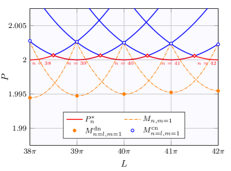
Figure 5: (Color online) Bifurcation thresholds in the $(L,P)$ plane: primary bifurcation thresholds $P_{n}^{*}$ to periodic states $\phi_{n}$ together with secondary bifurcation thresholds $M_{n,m=1}$ to dnoidal states (dash-dotted lines) obtained by numerical continuation, each for $n=38,39,...,42$. The symbol $\diamond$ denotes codimension-two transitions between $n$ and $n+1$ periodic wrinkle states. The red filled (resp. blue open) circles indicate the multiscale analysis predictions of bifurcations to dnoidal (resp. cnoidal) states when $n=l$ (with $l=L/\pi\in\mathbb{Z}^{+}$).

As shown in Fig. 5 the multiscale analysis generates a discrete set of bifurcation points instead of the continuous curves of bifurcation points obtained by numerical continuation. The solid curves for $L\in(l\pi,(l+1)\pi)$, $l\in\mathbb{Z}^{+}$, can only be obtained via numerical continuation. This limitation of the multiscale analysis has its origin in the structure of the equations analyzed in Sec. II.1, which requires $l\in\mathbb{Z}^{+}$ to satisfy simultaneously the boundary conditions and the cancellation of the right-hand side of the $\mathcal{O}\left(\epsilon^{2}\right)$ equation in Eq. (16). If we instead follow (Audoly, 2011; Oshri et al., 2015) and minimize the functional $\overline{G}$ on the assumption that $y(s)=A(S)\cos(qs)$ we obtain Eq. (17) when $q=1$ and a similar equation to Eq. (17) but with $q$-dependent coefficients whenever $q>1$. The latter, however, yields inaccurate solutions, which are an artifact of improper assumption on the $s$-dependence of $y(s)$ when $q>1$.

II.3 The $\pi/2$-shifted localized branch

The exact nonlinear solutions in Eqs. (5)–(6) show that the symmetric and antisymmetric folds on an infinite sheet are equivalent from the energy point of view. Such states are therefore energetically degenerate. However, this is no longer the case on a finite sheet and the question arises whether whether a sheet whose wrinkle-to-fold transition yields a symmetric (antisymmetric) fold may also display an antisymmetric (symmetric) fold. Results from Sec. II.1.2 provide hints about the dynamical features of these two states. For $l\in\mathbb{Z}^{+}$ symmetric and antisymmetric single fold states (i.e., $n=l,m=1$) can be understood in terms of the carrier wave phase $\theta$. The idea is simple: since both Jacobi elliptic functions of the approximate solutions in Table 2 have a maximum at the center of the sheet, the choice of whether $\theta=0$ or $\theta=\pi/2$ determines the symmetry of the central fold. For $n=l$ even (odd), the dnoidal (cnoidal) branch yields the antisymmetric (symmetric) single fold state and the cnoidal (dnoidal) branch the symmetric (antisymmetric) state. However, there is an important difference between these two branches. The cnoidal branch, whose carrier wave is shifted by $\pi/2$ relative to the dnoidal branch, emerges from the trivial state through a primary bifurcation to the right of the primary bifurcation to the periodic state (and half as close to it as the dnoidal branch bifurcation on the left). The resulting predictions of the theory of Sec. II.1.2 are displayed in the inset of Fig. 3(a) and compared there with the corresponding results from numerical continuation. The accuracy of the approach is very good.

The theoretical predictions show that in the limit $L\rightarrow\infty$ both branches merge into a single one in terms of $\left(\Delta,E,G,P\right)$. As $L$ increases, the secondary bifurcation to dnoidal states is pushed downward along the primary periodic branch while the cnoidal bifurcation point is also pushed towards the primary bifurcation point. These two bifurcation points coalesce in the limit $L\rightarrow\infty$. The corresponding large amplitude dnoidal and cnoidal branches become rapidly very close as $P$ decreases, a prediction that is confirmed by numerical continuation to values of $\epsilon$ far beyond $\epsilon=1$, i.e., $P\ll 1$.

II.4 Multifold solutions

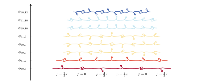
Figure 6: (Color online) A set of spatially modulated periodic solutions from numerical continuation for a sheet of length $L=40\pi$ and different values of $n$ and $m$. In all cases $P=1$. The solutions are composed of distorted folds. While $m$ determines the number of folds, $n$ fixes the shape of each fold (see text for details). For the lowest state, the local phase of the carrier wave, $\varphi_{f}$, is indicated.

The modulation analysis carried out above also provides a clearer picture of the emergence of multifold ($m\geq 2$) solutions for $l\equiv(L/\pi)\in\mathbb{Z}^{+}$. The condition $q=1$ requires that $n=l$, where the labels $n$ and $m$, introduced in Sec. II.0.1, represent the carrier and envelope wave numbers, respectively. The bifurcations for $m\geq 2$ follow the same principle as the branches of localized states when $m=1$, i.e., the dnoidal $m$-branch bifurcates from a periodic state $\phi_{n}$ at finite amplitude while the corresponding cnoidal $m$-branch bifurcates from the periodic state $\phi_{n+m}$ at a very small amplitude, and to the right of the primary bifurcation to $\phi_{n}$ and half as close to it as the bifurcation to the dnoidal branch. For example, when $m=2$ the cnoidal branch in general bifurcates from $\phi_{42}$ and does so very close to the point $P_{42}^{*}$, although it may bifurcate directly from the trivial state but only at the crossing point of $P_{38}^{*}$ and $P_{42}^{*}$. Likewise, the bifurcation points to the $m\geq 2$ dnoidal branches spread out from the primary bifurcation point to the $n$th periodic branch as $m^{2}$. We also used numerical continuation to follow the $M_{n,m}$ bifurcation points as a function of $L$ as done in Sec. II.2 for $M_{n,1}$. Just as the single-fold cnoidal bifurcation point lies in the vicinity of $L_{\left(n-1,n+1\right)}$, the crossing point of the primary bifurcations to the $n-1$ and $n+1$ periodic branches, the $m$-fold cnoidal bifurcation point is located in the vicinity of $L_{\left(n-m,n+m\right)}$, the crossing point of the primary bifurcations to the $n-m$ and $n+m$ periodic branches. Likewise, the $M_{n,m}$ bifurcation curves for noninteger $L/\pi$ resemble parabolas with vertices near $M_{l=n,m}^{\,\mathrm{dn}}$ extending from $L_{(n-2m,n)}$ to $L_{(n,n+2m)}$. The range of existence of the parabola clarifies why the number of $m$-fold states observed is $2m+2$ and which $n$ values are allowed for a given $m$ and $L$.

The analysis also reveals another interesting feature. The choice of $l$ and $m$ determines (a) if the solution consists of an array of symmetric or antisymmetric folds, and (b) the local shape of each fold. The rule for (a) is very simple: these states are allowed if $l$ is divisible by $m$. For the dnoidal solutions, if $l/m$ is even, the solutions will be an array of antisymmetric folds whereas for $l/m$ odd the solution will be an array of symmetric folds with alternating orientation. If folds are allowed at both boundaries, another possible solution, consisting of alternating antisymmetric folds for $l/m$ even, can be observed. For $l=40$, periodic multifold states are observed for $m=2,4,5,8,10,20$, as displayed in Fig. 4 ($m=20$ is not shown). The figure also shows a state with folds at either boundary, for $m=8$, to illustrate the complementary family of periodic solutions.

When $l$ is not divisible by $m$ the folds forming the array become distorted and resemble the family of arbitrary phase folds described in (Rivetti, 2013) for an infinite length sheet. The rule (b) for the local shape of each fold can be understood in terms of the phase $\varphi_{f}$ in Eq. (7), which is now fixed by the carrier wave. The $j$th fold of the dnoidal solutions displays a local phase $\varphi_{f}=-l\pi\left(j-1/2\right)/m$, whereas for the cnoidal solutions $\varphi_{f}=-\pi/2-l\pi\left(j-1/2\right)/m$. Accordingly, the fundamental period of an array of folds in a dnoidal solution is given by $2L/\mbox{GCD}\left(l,2m\right)$ while the fundamental period for cnoidal solutions is $L/\mbox{GCD}\left(l,m\right)$ provided $l$ is divisible by $m$ and $l/\mbox{GCD}\left(l,m\right)$ is odd, or $2L/\mbox{GCD}\left(l,m\right)$ in all other cases. Examples of distorted folds are displayed in Fig. 6 for $L=40\pi$. Solutions which do not satisfy $q=1$, e.g., $\phi_{n=39,m}$ or $\phi_{n=41,m}$ in a $L=40\pi$ domain, obey a similar rule for the local phase as that obtained by swapping the integer $l$ for $n$, i.e., replacing $l$ in $\varphi_{f}$ by $n$ to obtain $\phi_{n\neq l,m}$. Further analysis for this general case is required to understand this feature.

II.5 Discussion

II.5.1 Energy gap

The energy of the dnoidal and cnoidal branches for $l\in\mathbb{Z}^{+}$ and $n=l$ far from the bifurcation can be found by expanding the expressions for $P$, $\overline{G}$, $\overline{\Delta}$ and $\overline{E}$ obtained in Sec. II.1.2 around $k=1$. If we write $k=1-\xi$, $\xi\ll 1$, we obtain

$$g_{m}\equiv\frac{1}{m}G_{m}^{\pm}\left(P\right) = \frac{8}{3}\left(2-P\right)^{3/2}\left(1\mp\frac{3}{2}\xi\right),$$ (29)

$$e_{m}\equiv\frac{1}{m}E_{m}^{\pm}\left(\Delta\right) = 2\delta_{m}-\frac{1}{48}\delta_{m}^{3}\left(1\mp 3\xi\right),$$ (30)

where the $-$ ($+$) corresponds to the dnoidal (cnoidal) branch and $\delta_{m}\equiv\Delta/m$ is a single-fold average compression. Notice that the results are no longer expressed in terms of mean values. At leading order both branches have exactly the same energy. Equation (29) shows that, for fixed $P$ (dead loading), the $G$ spectrum is a set of equispaced free energies, where the quantity $g_{m}\approx\frac{8}{3}\left(2-P\right)^{3/2}$ can be identified with the free energy of a single fold. On the other hand, for fixed compression $\Delta$ (rigid loading), the energy of a single fold is $e_{m}\approx 2\delta-\delta^{3}/48$. The energies display maxima at $\delta_{\max}=2^{5/2}$, with $e_{\max}=2^{9/2}/3$. Numerical continuation shows that this point is related to self-contact of the sheet. A comparison between the numerical results and the analytical approach at leading order is shown in Fig. 7 for $q=1$. The overlap between the numerical continuation results and the analytical approximation is remarkable.

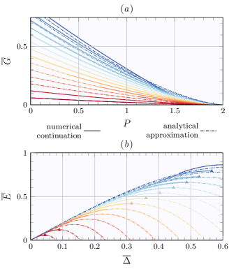
Figure 7: (Color online) Multifold branches for a sheet of length $L=40\pi$ over a fluid substrate in (a) the $\left(P,\overline{G}\right)$ plane and (b) the $\left(\overline{\Delta},\overline{E}\right)$ plane. Solid lines represent the numerical continuation results while the dash-dotted lines indicate the leading order analytical approximation. The numerical continuation was stopped at $P=0$ [indicated by $\blacktriangle$ in (b)] in all cases, although the analytical approach extends beyond this point. The analytical approximation starts to depart from the numerical results only when the number of folds is very high, $m>10$.

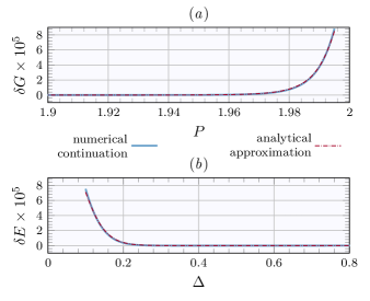
Figure 8: (Color online) Gap between the dnoidal and cnoidal single fold solutions for $L=40\pi$ in (a) the $\left(P,G\right)$ plane and (b) the $\left(\Delta,E\right)$ plane. The analytical approximation (dash-dotted line) once again matches the numerical continuation results (solid line).

Figure 8 shows the difference between the $m=1$ dnoidal and cnoidal branches obtained from numerical continuation and compares the result with a theoretical prediction obtained by inverting the series expansions for either $P$ or $\Delta$ to obtain $\xi$ in terms $P$ or $\Delta$. The final result for the energy gap between the dnoidal and cnoidal branches is

$$\delta g_{m} \equiv g_{m}^{+}-g_{m}^{-}=-64\left(2-P\right)^{\frac{3}{2}}\mathrm{e}^{-\frac{1}{2}l_{m}\left(2-P\right)^{\frac{1}{2}}},$$ (31)

$$\delta e_{m} \equiv e_{m}^{+}-e_{m}^{-}=-\delta_{m}^{3}\mathrm{e}^{-\frac{1}{8}l_{m}\delta_{m}},$$ (32)

where $l_{m}\equiv L/m$ can be identified as the spacing between the folds. The predicted exponential decay in both $\left(P,G\right)$ and $\left(\Delta,E\right)$ planes matches the numerical results almost perfectly. The exponentially small residual difference is a consequence of the finite sheet size and can be understood as the interaction between the exponential tails of localized solutions (Kozyreff and Chapman, 2006).

The general case $q\neq 1$ far from the bifurcation is more complicated and is not well described by the weak modulation approach. Numerical continuation shows that, at leading order, the energies for $q\neq 1$ are in fact exactly the same as those for the $q=1$ branches: the solutions appear to shift their $q$ towards $q=1$ as $k\rightarrow 1$, a feature that is beyond the scope of the approach in Sec. II.1.

II.5.2 Stability analysis

The analysis carried out in the previous sections provides a framework for understanding how single fold and multifold solutions bifurcate from periodic states. However, this type of analysis does not address the stability of the solutions, although we expect solutions with lowest energy such as the single fold solution $\phi_{40,1}$ for $L=40\pi$ to be stable. For example, it may happen that several solutions are stable simultaneously. Thus a stability analysis provides a link between the theoretical predictions and observations in experiments.

To explore the stability properties of the solutions identified above, we carried out a numerical study based on a variational approach. Since the equations of a fluid-supported elastic sheet are static (time-independent), we consider a solution as stable if and only if it corresponds to a local minimum of energy in the space of functions satisfying all the constraints, as well as the boundary and symmetry conditions imposed by the problem formulation. The stability of a solution is thus guaranteed if the energy functional is positive definite in its vicinity, i.e., if and only if $E\left[\phi_{0}+\delta\phi\right]>E\left[\phi_{0}\right],\;\forall\,\delta\phi\,\in\,\mathbb{F}_{\phi}$, where $E$ is defined as in Eq. (1), $\phi_{0}$ is the solution under study, $\delta\phi\neq 0$ is the variation of $\phi_{0}$ and $\mathbb{F}_{\phi}$ is the space of (continuous) functions such that $\phi_{0}+\delta\phi$ satisfies the prescribed constraints (e.g. $\Delta\left[\delta\phi\right]=0$ under rigid loading), and the boundary and symmetry conditions (hinged, symmetric or antisymmetric).

We define the inner product $\left(f,g\right)\equiv\int_{-L/2}^{L/2}f\cdot g\,\mathrm{d}s=\int_{-L/2}^{L/2}f^{\dagger}g\,\mathrm{d}s$. It can be shown (see Appendix B) that the functionals $E,G$ evaluated at $y=y_{0}+\delta y$ can be written as

$$E\left[y\right]= E_{0}+\left(\frac{\delta E}{\delta y},\delta y\right)+\left(\delta y,\frac{\delta^{2}E}{\delta y}\delta y\right)+\mathcal{O}\left(\delta y^{3}\right),$$

$$G\left[y\right]= G_{0}+\left(\frac{\delta G}{\delta y},\delta y\right)+\left(\delta y,\frac{\delta^{2}G}{\delta y}\delta y\right)+\mathcal{O}\left(\delta y^{3}\right),$$

where $E_{0}=E\left[\phi_{0}\right]$, $G_{0}=G\left[\phi_{0}\right]$ and all the functional derivatives are evaluated at $\phi_{0}$ (equivalently, $y=y_{0}$). The variation $\delta y$ is related to the corresponding variation $\delta\phi$ by the geometrical relation $\partial_{s}\left(y+\delta y\right)=\sin\left(\phi+\delta\phi\right)$ (see Appendix B for further details). Similar relations can be written for $P$ and $\Delta$. By construction, the terms in $E$ or $G$ linear in $\delta y$ vanish when $y=y_{0}$ is a solution of the original variational problem. Hence, under dead loading ($P$ fixed) the solution is stable provided

$$\left(\delta y,\frac{\delta^{2}G}{\delta y^{2}}\delta y\right)=\left(\delta y,\left[\frac{\delta^{2}E}{\delta y^{2}}-P_{0}\frac{\delta^{2}\Delta}{\delta y^{2}}\right]\delta y\right)>0.$$

Here $P_{0}=P[y_{0}]$. In the rigid loading case, $P$ is no longer fixed and the stability condition becomes

$$\left(\delta y,\left[\frac{\delta^{2}E}{\delta y^{2}}-P_{0}\frac{\delta^{2}\Delta}{\delta y^{2}}\right]\delta y\right)-\delta P\left(\frac{\delta\Delta}{\delta y},\delta y\right)>0$$

with an extra constraint imposed by the fixed compression:

$$\left(\frac{\delta\Delta}{\delta y},\delta y\right)=0.$$

Since the operator $\delta^{2}G/\delta y^{2}$ in the square brackets is a real symmetric operator, the inner products behave as a quadratic form in function space. Thus, the spectral decomposition of the operator yields a set of eigenvalues and the corresponding eigenfunctions containing information about the stability of the solution.

In practice, we first recovered $\phi_{0}$ and the corresponding $y_{0}$ from the AUTO${}^{\text{©}}$ calculations and resampled them into an $N$ vector. The derivative operators from Eqs. (35)-(37) were likewise discretized into $N\times N$ arrays using Fourier derivative matrices. Using these results, we built a discrete $N\times N$ matrix of the free energy functional $\delta^{2}G/\delta y^{2}$, $\mathbf{G}_{N\times N}$. The stability of solutions in the dead loading case simply depends on the spectral decomposition of $\mathbf{G}_{N\times N}$, that is, on the eigenvalues of the standard eigenvalue problem

$$\mathbf{G}\left[\delta y\right]=\lambda\left[\delta y\right].$$ (33)

The rigid loading case requires further work because of the extra constraint. In this case we discretized the compression condition by introducing a matrix $\Delta_{N\times 1}^{\prime}$ as the discrete version of $\delta\Delta/\delta y$, and the ${\left(N+1\right)\times\left(N+1\right)}$ bordered Hessian matrix $\mathbf{H}$ given by

$$\mathbf{H}\equiv\left[\begin{array}[]{rr}0&-\mathbf{\Delta}_{1\times N}^{\prime}\\ -\mathbf{\Delta}_{N\times 1}^{\prime}&\mathbf{G}_{N\times N}\end{array}\right].$$

As shown in (A. C. Chiang and K. Wainwright, 2013), the stability problem can be studied via the generalized eigenvalue problem

$$\mathbf{H}\left[\begin{array}[]{c}\delta P\\ \delta y\end{array}\right]=\lambda\left[\begin{array}[]{ll}0&\bm{0}_{1\times N}\\ \bm{0}_{N\times 1}&\bm{I}_{N\times N}\end{array}\right]\left[\begin{array}[]{c}\delta P\\ \delta y\end{array}\right].$$ (34)

Thus the stability of a solution under dead or rigid loading can be tested by checking the signs of the eigenvalues of the standard (Eq. 33) or generalized eigenvalue (Eq. 34) problems, respectively. If all the eigenvalues are positive, linear stability is guaranteed.

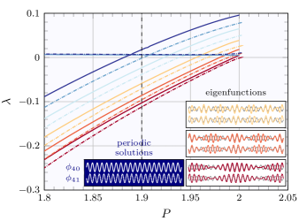
Figure 9: (Color online) Eigenvalues $\lambda$ as a function of the load $P$ for two periodic solutions: $\phi_{40}$ (solid lines) and $\phi_{41}$ (dash-dotted lines). The left inset shows the periodic solutions evaluated at $P=1.9$ (vertical dashed line in main panel). The right insets show the eigenfunctions evaluated at the same value of $P$ using the same color scheme as in the main panel. The $\phi_{40}$ eigenfunctions are displayed at the top (thick lines) and the $\phi_{41}$ eigenfunctions at the bottom (thin lines). The corresponding periodic solutions are plotted in black in the background for reference.

Within this framework, we now proceed to describe the stability properties of the solutions for a $L=40\pi$ sheet. Under dead loading, all the solutions described so far are unstable to amplitude modes, which is as expected as $\partial G/\partial P<0$ for all the branches studied. The rigid loading case is much more interesting, however. In the following section, we describe the stability properties of the periodic solutions $\phi_{40}$ and $\phi_{41}$, the symmetric and asymmetric single fold solutions $\phi_{40,1}$ and $\phi_{41,1}$, and the two-fold solutions $\phi_{39,2}$, $\phi_{40,2}$, $\phi_{41,2}$ and $\phi_{42,2}$. For the sake of completeness, we also examined the stability of solutions displaying half-folds at the boundaries, which we denote by the superscript $b$. For instance, the solution $\phi_{40,1}^{\left(b\right)}$ has half-folds at $s=\pm L/2$, i.e., $\frac{1}{2}$+$\frac{1}{2}$=1 complete fold.

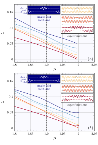
Figure 10: (Color online) Eigenvalues $\lambda$ as a function of the load $P$ for four single fold solutions. (a) Symmetric fold: $\phi_{40,1}$ (solid lines) and $\phi_{40,1}^{\left(b\right)}$ (dash-dotted lines). (b) Antisymmetric fold: $\phi_{41,1}$ (solid lines) and $\phi_{41,1}^{\left(b\right)}$ (dash-dotted lines). As in Fig. 9, the left insets show the solutions evaluated at $P=1.9$ and those on the right show the eigenfunctions. The centered fold eigenfunctions are displayed at the top (solid lines) and the boundary half-fold eigenfunctions at the bottom (dashed lines).

II.5.3 Stability of periodic solutions

Figure 9 shows the six lowest eigenvalues $\lambda$ as a function of the load $P$ for the periodic solutions $\phi_{40}$ (solid lines) and $\phi_{41}$ (dashed lines). The corresponding eigenfunctions evaluated at $P=1.9$ are shown in the right insets following the same color scheme as used for the eigenvalues. The figure indicates that the periodic solution $\phi_{40}$ becomes unstable at $P=1.995$, when its lowest eigenvalue becomes negative. The corresponding eigenfunction represents a buckling mode that leads to either a centered single fold state or a pair of half-folds on the boundaries. We will refer to these eigenfunctions as fold eigenmodes. At $P\approx 1.980,$ a second eigenvalue becomes negative, which buckles the solution into a pair of folds (or a $\frac{1}{2}$+1+$\frac{1}{2}$-fold state); at $P\approx 1.956$, a third instability sets in, buckling the solution into three folds or a $\frac{1}{2}$+1+1+$\frac{1}{2}$-fold state, etc. The points where these solutions cross $\lambda=0$ are consistent with the branch points identified using AUTO${}^{\text{©}}$ as leading to solutions that subsequently evolve into fold solutions. Similar behavior is observed for the periodic solution $\phi_{41}$, with fold eigenvalues crossing $\lambda=0$ sequentially as the number of folds increases. Besides the fold eigenvalues all of which decrease monotonically as $P$ decreases, a second family of eigenvalues is also present. However, these never cross $\lambda=0$ even though they decrease monotonically as $P$ decreases. The associated eigenfunctions do not buckle the solution into localized folds but instead introduce spatial modulation on top of the periodic pattern. We conclude that the periodic solutions are stable with respect to spatial modulation, at least when the wavelength of the periodic state is close to the natural wavelength (no Eckhaus instability).

Figure 12(a) shows the construction of a $n=40$ pseudo-solution arising from the second unstable fold mode. The pseudo-solution is obtained by adding a multiple of the eigenfunction (here the multiple is $\pm 1$) to the periodic state $\phi_{40}$. Panel (a) shows that when the multiple is $+1$ the instability suppresses the oscillations in the center and near the boundaries, leaving a $1+1$ state. When the multiple is $-1$ the result is a state resembling a $\frac{1}{2}$+1+$\frac{1}{2}$ state.

II.5.4 Stability of single fold solutions

The corresponding diagram for single fold solutions is shown in Fig. 10. The four single fold solutions have positive eigenvalues and hence are all stable. The first two solutions $\phi_{40,1}$ and $\phi_{40,1}^{\left(b\right)}$, have identical eigenvalues, a consequence of the fact that $\phi_{40,1}^{\left(b\right)}$ can be obtained through a half-domain translation of $\phi_{40,1}$. This translation respects the boundary conditions at $s=\pm L/2$. The lowest eigenvalue of $\phi_{40,1}$ is inherited from the periodic branch $\phi_{40}$ and represents the amplitude mode of $\phi_{40}$ [Fig. 12(b)]. The second lowest eigenvalue is of particular interest, because its eigenmode is related to the splitting of the central fold into two [Fig. 12(c)]. These eigenmodes, which will be referred to as splitting eigenmodes, represent modulation of a carrier wave that shifts continuously with respect to the base state, with a $\pi$-phase shift at the center of the fold. With increasing amplitude this mode leads to growing separation of the central fold into two adjacent folds, in contrast to the usual fold eigenmodes corresponding to a $0$ or $\pi$ shift. The third eigenvalue is linked to a fold eigenmode which buckles the solution into a $\frac{1}{2}$+$1$+$\frac{1}{2}$ array. Larger eigenvalues show similar behavior involving larger numbers of folds. However, none of these modes is unstable, and so no finite amplitude solutions of this type are present.

The stability behavior the $\phi_{41,1}$ state is similar to that of $\phi_{40,1}$ although there are some important differences. First, the solution $\phi_{41,1}^{\left(b\right)}$ no longer corresponds to a simple half-domain shift of $\phi_{41,1}$: to satisfy symmetry conditions, a $\frac{\pi}{2}$ phase shift of the carrier wave plus an inversion of the solution in one half of the domain is also required. As a result the eigenvalues of $\phi_{41,1}$ and $\phi_{41,1}^{\left(b\right)}$ are no longer identical. The slight difference between them ($\lesssim 10^{-4}$) is due to the presence of a defect in the center of the domain in the latter case. The lowest eigenvalue mode is again related to the periodic solution, $\phi_{41,0}$. The next lowest eigenvalue mode is now a $1$+$1$ eigenmode while the third is a splitting eigenmode. Notice also that the second mode has the lowest eigenvalue for $P\lessapprox 1.982$ but this eigenvalue, like the others, remains positive and no instability is triggered.

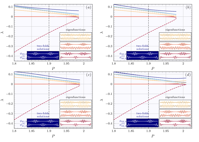
Figure 11: (Color online) Eigenvalues $\lambda$ as a function of the load $P$ for the eight two-fold solutions. (a) $\phi_{39,2}$ (solid lines) and $\phi_{39,2}^{\left(b\right)}$ (dash-dotted lines). (b) $\phi_{40,2}$ (solid lines) and $\phi_{40,2}^{\left(b\right)}$ (dash-dotted lines). (c) $\phi_{41,2}$ (solid lines) and $\phi_{41,2}^{\left(b\right)}$ (dash-dotted lines). (d) $\phi_{42,2}$ (solid lines) and $\phi_{42,2}^{\left(b\right)}$ (dash dotted lines). As in Fig. 9, the left insets show the solutions evaluated at $P=1.9$ and those on the right show the eigenfunctions. The centered fold eigenfunctions are displayed at the top (solid lines) and boundary half-fold eigenfunctions at the bottom (dashed lines).

II.5.5 Stability of two-fold solutions

We also studied the stability properties of the two-fold solutions. The eigenvalues of the $\phi_{39,2}$, $\phi_{40,2}$, $\phi_{41,2}$ and $\phi_{42,2}$ solutions are shown in Fig. 11 (solutions with folds on the boundaries are also shown). All the two-fold solutions are unstable displaying a single negative eigenvalue. At the bifurcation point to a two-fold solution (e.g. at $P\approx 1.98$ for $\phi_{39,2}$) the amplitude eigenvalue inherited from the periodic state vanishes but becomes positive as $P$ decreases just as in the single fold case. However, this eigenvalue is passed by that of another mode in the vicinity of the bifurcation point (e.g. at $P\lessapprox 1.975$ for $\phi_{39,2}$). The corresponding eigenmode is non-periodic and remarkably interesting. For the $\phi_{41,2}$ and $\phi_{42,2}$ solutions, these two lowest eigenvalue modes display the same modulation as the periodic solution but with a $\pm\frac{\pi}{2}$ shift in the carrier wave. Because of the localization of the folds, this feature is a reminiscent of a Goldstone translation mode. The eigenmode acts on the solutions by translating the left fold to the right ($+\frac{\pi}{2}$ shift) and the right fold to the left ($-\frac{\pi}{2}$ shift), or vice versa, without changing their shape. Consequently we refer to this mode as an translational attraction (or repulsion) eigenmode. The other lowest eigenvalue mode is slightly different: on a one side of a fold the mode displays a $\pi$ shift while on the other side there is no phase shift. These eigenmodes also generate attraction (or repulsion) between folds but also change their shape. We refer to them as rolling attraction (or repulsion) eigenmodes. While in the translation mode both the carrier wave and the envelope translate, in the rolling case only the envelope shifts, resulting in a local deformation of the folds. The situation for $\phi_{39,2}$ and $\phi_{40,2}$ is similar with the difference that the translation and rolling eigenmodes change their order. Figures 12(d) and (e) show pseudo-solutions that indicate the tendencies represented by these modes. We conclude that the two-fold states are in all cases unstable and that the instability takes the form of a gradual approach of the two folds, ultimately resulting in a stable single fold state. The manifestation of the instability may be very slow, however, as it depends on the energy difference between these two states. This conclusion is supported by the fact that the unstable eigenvalue of the two-fold state approaches zero from below, asymptotically exponentially, as $P$ decreases. This comes as no surprise since the two folds can only interact via the overlapping tails of their profiles and these are exponentially small when the folds are sufficiently far apart, a fact that suggests that as the solutions increasingly localize (i.e., $P$ decreases), the time required for the system to reach the single fold state becomes exponentially long. This decay may arise through attraction via either the translation or rolling eigenmodes. In contrast, two-fold solutions with folds on the boundary decay into a single fold state much more rapidly as the folds at the boundary decay leaving only the fold at the center.

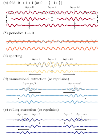
Figure 12: (Color online) Examples of base states (top solid lines) and the corresponding eigenmodes (top dash-dotted lines) and pseudo-solutions obtained by their superposition (bottom lines). (a) Periodic solution (red) and the fold eigenmode (black) superposed in two ways. (b) Single fold solution (orange) and the periodic eigenmode (gray). (c) Single fold solution (yellow) and the splitting eigenmode (gray). (d) Two-fold solution (gray) and the translational attraction/repulsion eigenmode (blue). (e) Two-fold solution (blue) and the rolling attraction/repulsion eigenmode (gray).

III Conclusions

In this article, we reported on the existence of multifold solutions in a thin floating elastic sheet of finite length with hinged boundary conditions. Starting from known large amplitude periodic solutions Oshri et al. (2015), we used numerical continuation to uncover a series of solution branches that bifurcate from the periodic (wrinkle) branch as a function of the load $P$ or the associated compression $\Delta$. Each branch consists of an array of localized (fold) solutions. Symmetric and antisymmetric single fold solutions, which are well known for the infinite sheet case Diamant and Witten (2013), are found to bifurcate from branches of distinct periodic states and inherit their symmetry properties. The multifold states with $m=2,3,\dots$ folds in the domain bifurcate from the periodic states in subsequent bifurcations and are, we believe, new.

Based on our numerical continuation results, we performed a weakly nonlinear analysis of the multifold solutions. These states form as a result of a slow spatial modulation of the periodic wrinkle solutions. The spatial modulation satisfies an amplitude equation whose solutions can be written down in terms of Jacobi elliptic functions. The results determine the branches of multifold solutions in the parameter space and match the numerical continuation results remarkably well. In particular, we determined the energy of multifold states and showed that the energies of like-number multifold states are almost equal, with energy gaps that become exponentially small as the sheet length increases (see Eq. (30)).

Finally, we also studied the stability of both the periodic and multifold solutions within a variational framework. We showed numerically that the symmetric and antisymmetric single fold solutions are both stable, but that only one of them bifurcates from a stable periodic branch and so inherits its stability. We also showed that all the two-fold solutions are unstable, but with a common instability mode characterized by the mutual attraction/repulsion of folds (see Sec. 11). However, the relevant eigenvalue comes very close to zero as the localization increases, implying that the transition to a single fold state requires essentially exponentially long times. This result is in agreement with the numerical simulations in Marple et al. (2015) (with clamped boundary conditions) in which a three-fold state is observed to decay into a single fold state but did so so slowly that it was thought to be stable.

These results have been obtained for the special case of hinged boundary conditions. However, some numerical experiments employ clamped boundary conditions, see e.g. Rivetti and Neukirch (2014), and in this case the route to localization appears to be different. Thus an extension of the type of analysis performed here to the case of clamped boundary conditions $\phi=\phi^{\prime\prime}=0$ at $s=\pm L/2$ would also be valuable.

Our results can be used to provide a rule of thumb for experiments employing hinged boundary conditions where localization of wrinkles into folds is crucial. Multifold solutions may emerge naturally in certain geometries (for instance, in a floating elastic annulus or an indented circular sheet Paulsen et al. (2016, 2017)). The prediction of the energy gap between multifold and single fold states obtained here can be used to determine which states can emerge deterministically or stochastically in the presence of thermal noise. This is of particular importance in microscopic-scale experiments Gopal et al. (2006); Leahy et al. (2010) and in experiments in which the floating raft is granular Jambon-Puillet et al. (2017). Although in most experiments folds are allowed to form spontaneously, our calculations also provide a basis for predicting the outcome of experiments with manually induced folds, which may be of particular interest in technological applications.

Appendix A Jacobi elliptic integrals

The quantities related to $A$ in Sec. II.1.2 can be written in terms of fundamental Jacobi elliptic integrals,

$$\left(\overline{A\,_{\,\mathrm{dn}}^{2}},\overline{A\,_{\,\mathrm{cn}}^{2}}\right) = 2^{4}\kappa^{2}\left(D_{2},C_{2}\right),$$

$$\left(\overline{A_{\,\mathrm{dn}}^{{}^{\prime}2}},\overline{A_{\,\mathrm{cn}}^{{}^{\prime}2}}\right) = 2^{4}\kappa^{4}(D{}_{2}^{{}^{\prime}},C{}_{2}^{{}^{\prime}}),$$

$$\left(\overline{A\,{}_{\,\mathrm{dn}}^{4}},\overline{A\,{}_{\,\mathrm{cn}}^{4}}\right) = 2^{8}\kappa^{4}\left(D_{4},C{}_{4}\right),$$

where the coefficients $D_{2},C_{2},D{}_{2}^{{}^{\prime}},C{}_{2}^{{}^{\prime}},D_{4},C_{4}$ are given, respectively, by the following mean values of the Jacobi elliptic functions:

$$\begin{array}[]{ccccl}D_{2}&\equiv&\overline{\,\mathrm{dn}_{k}^{2}}&=&1-I(k)\\ D_{2}^{{}^{\prime}}&\equiv&\overline{\,\mathrm{dn}_{k}^{{}^{\prime}2}}&=&\frac{1}{3}\left[k^{2}-\left(2-k^{2}\right)I(k)\right]\\ D_{4}&\equiv&\overline{\,\mathrm{dn}_{k}^{4}}&=&\frac{1}{3}\left[\left(3-k^{2}\right)-2\left(2-k^{2}\right)I(k)\right]\\ C_{2}&\equiv&\overline{k^{2}\,\mathrm{cn}_{k}^{2}}&=&k^{2}-I(k)\\ C_{2}^{{}^{\prime}}&\equiv&\overline{k^{2}\,\mathrm{cn}_{k}^{{}^{\prime}2}}&=&\frac{1}{3}\left[k^{2}-\left(2k^{2}-1\right)I(k)\right]\\ C_{4}&\equiv&\overline{k^{4}\,\mathrm{cn}_{k}^{4}}&=&\frac{1}{3}\left[k^{2}\left(3k^{2}-1\right)-2\left(2k^{2}-1\right)I(k)\right].\end{array}$$

Appendix B Expansion of functionals

Consider a small perturbation of a solution $y_{0}$ satisfying the variational problem, $y=y_{0}+\delta y$, where $\delta y$ is assumed to be of order $\varepsilon$, i.e. $\delta y=\varepsilon y_{1}\neq 0$ and $y_{1}\sim\mathcal{O}\left(1\right)$:

$$y = y_{0}+\varepsilon y_{1}.$$

The function $\phi\left(s\right)$ can be expanded in terms of $\varepsilon$,

$$\phi=\phi_{0}+\varepsilon\phi_{1}+\varepsilon^{2}\phi_{2}+\ldots$$

and likewise for the load $P$,

$$P = P_{0}+\varepsilon P_{1}+\ldots$$

and the compression and energy functionals,

$$\Delta = \Delta_{0}+\varepsilon\Delta_{1}+\varepsilon^{2}\Delta_{2}+\ldots$$

$$E = E_{0}+\varepsilon E_{1}+\varepsilon^{2}E_{2}+\ldots$$

$$G = G_{0}+\varepsilon G_{1}+\varepsilon^{2}G_{2}+\ldots$$

Each term in these expansions can be obtained from the definitions of these relevant quantities (Sec. I.1). For instance, the function $\phi$ is related to $y$ through $\dot{y}=\sin\phi$, and it can be shown that the first and second order terms in the expansion of $\phi$ are, respectively,

$$\phi_{1} = \sec\phi_{0}\,\partial_{s}y_{1},$$

$$\phi_{2} = \frac{1}{2}\tan\phi_{0}\sec^{2}\phi_{0}\left(\partial_{s}y_{1}\right)^{2}.$$

Analogously, the functionals $\Delta$ and $E$ can be written as

$$\Delta =\Delta_{0}+\varepsilon\left(\frac{\delta\Delta}{\delta y},y_{1}\right)+\varepsilon^{2}\left(y_{1},\frac{\delta^{2}\Delta}{\delta y}y_{1}\right)$$

$$E =E_{0}+\varepsilon\left(\frac{\delta E}{\delta y},y_{1}\right)+\varepsilon^{2}\left(y_{1},\frac{\delta^{2}E}{\delta y}y_{1}\right),$$

where $\Delta_{0}$ and $E_{0}$ and their functional derivatives are evaluated at the solution $y_{0}$. For the sake of simplicity, we only consider here the terms that are relevant for the stability analysis. For the displacement, we obtain:

$$\frac{\delta\Delta}{\delta y} =\tan\phi_{0}D_{s},$$ (35)

$$\frac{\delta^{2}\Delta}{\delta y^{2}} =D_{s}^{\dagger}\Sigma_{s}^{\Delta}D_{s},$$ (36)

while for the energy,

$$\frac{\delta^{2}E}{\delta y^{2}} =D_{ss}^{\dagger}\Sigma_{ss}^{E}D_{ss}-D_{s}^{\dagger}\Sigma_{s}^{E}D_{s}+\Sigma_{0}^{E},$$ (37)

where $D_{s}$ and $D_{ss}$ are, respectively, the first and second order linear differential operators and $D_{s}^{\dagger}$ and $D_{ss}^{\dagger}$ are the corresponding adjoint operators. The scalar operators $\Sigma_{s}^{D}$, $\Sigma_{ss}^{E}$, $\Sigma_{s}^{E}$ and $\Sigma_{0}^{E}$ are given by

$$\Sigma_{s}^{\Delta}\equiv \frac{1}{2}\sec^{3}\phi_{0},$$

$$\Sigma_{0}^{E}\equiv \frac{1}{2}\sec^{2}\phi_{0}\left(y_{0}\dot{\phi}_{0}+\cos\phi_{0}\right),$$

$$\Sigma_{s}^{E}\equiv \frac{1}{4}y_{0}^{2}\sec^{3}\phi_{0}+\ldots$$

$$\left[\dot{\phi_{0}}^{2}\left(\frac{1}{2}+\tan^{2}\phi_{0}\right)+\ddot{\phi}_{0}\tan\phi_{0}\right]\sec^{2}\phi_{0},$$

$$\Sigma_{ss}^{E}\equiv \frac{1}{2}\sec^{3}\phi_{0}.$$

A straightforward calculation shows that the free-energy second-order term $G_{2}$ is given by

$$G_{2}=\left(y_{1},\frac{\delta^{2}G}{\delta y}y_{1}\right)-P_{1}\left(\frac{\delta\Delta}{\delta y},y_{1}\right)$$

, where the second order functional derivative is simply

$$\frac{\delta^{2}G}{\delta y^{2}}=\frac{\delta^{2}E}{\delta y^{2}}-P_{0}\frac{\delta^{2}\Delta}{\delta y^{2}}.$$

Notice that the functional derivatives have been introduced in symmetrical form, which simplifies the numerical calculations of Sec. II.5.2.

References

- Pocivavsek et al. (2008) L. Pocivavsek, R. Dellsy, A. Kern, S. Johnson, B. Lin, K. Y. C. Lee, and E. Cerda, Science 320, 912 (2008).
- Diamant and Witten (2011) H. Diamant and T. A. Witten, Phys. Rev. Lett. 107, 164302 (2011).
- Audoly (2011) B. Audoly, Phys. Rev. E 84, 011605 (2011).
- Rivetti and Neukirch (2014) M. Rivetti and S. Neukirch, Journal of the Mechanics and Physics of Solids 69, 143 (2014).
- Oshri et al. (2015) O. Oshri, F. Brau, and H. Diamant, Phys. Rev. E 91, 052408 (2015).
- Hunt et al. (2000) G. W. Hunt, M. A. Peletier, A. R. Champneys, P. D. Woods, M. A. Wadee, C. J. Budd, and G. J. Lord, Nonlinear Dynamics 21, 3 (2000).
- Thompson and Champneys (1996) J. M. T. Thompson and A. R. Champneys, Proc. R. Soc. London A 452, 117 (1996).
- Champneys and Thompson (1996) A. R. Champneys and J. M. T. Thompson, Proc. R. Soc. London A 452, 2467 (1996).
- Champneys and Groves (1997) A. R. Champneys and M. D. Groves, J. Fluid Mech. 342, 199 (1997).
- Burke and Knobloch (2006) J. Burke and E. Knobloch, Phys. Rev. E 73, 056211 (2006).
- Knobloch (2015) E. Knobloch, Annu. Rev. Condens. Matter Phys. 6, 325 (2015).
- Iooss and Pérouème (1993) G. Iooss and M. Pérouème, J. Diff. Eq. 102, 62 (1993).
- Kozyreff and Chapman (2006) G. Kozyreff and S. J. Chapman, Phys. Rev. Lett. 97, 044502 (2006).
- Chapman and Kozyreff (2009) S. J. Chapman and G. Kozyreff, Physica D 238, 319 (2009).
- Gaivão and Gelfreich (2011) J. P. Gaivão and V. Gelfreich, Nonlinearity 24, 677 (2011).
- Bergeon et al. (2008) A. Bergeon, J. Burke, E. Knobloch, and I. Mercader, Phys. Rev. E 78, 046201 (2008).
- Burke and Knobloch (2009) J. Burke and E. Knobloch, Discrete and Continuous Dyn. Syst.-Suppl. September, 109 (2009).
- Peletier and Troy (2006) L. A. Peletier and W. C. Troy, Spatial Patterns: Higher Order Models in Physics and Mechanics (Basel: Birkhäuser, 2006).
- Burke and Knobloch (2007a) J. Burke and E. Knobloch, Phys. Lett. A 360, 681 (2007a).
- Burke and Knobloch (2007b) J. Burke and E. Knobloch, Chaos 17, 037102 (2007b).
- Rivetti (2013) M. Rivetti, Comptes Rendus Mécanique 341, 333 (2013).
- Marple et al. (2015) G. R. Marple, P. K. Purohit, and S. Veerapaneni, Phys. Rev. E 92, 012405 (2015).
- Cerda and Mahadevan (2003) E. Cerda and L. Mahadevan, Phys. Rev. Lett. 90, 074302 (2003).
- Brau et al. (2013) F. Brau, P. Damman, H. Diamant, and T. A. Witten, Soft Matter 9, 8177 (2013).
- Doedel et al. (1991a) E. Doedel, H. B. Keller, and J. P. Kernevez, Int. J. Bifurcat. Chaos 1, 493 (1991a).
- Doedel et al. (1991b) E. Doedel, H. B. Keller, and J. P. Kernevez, Int. J. Bifurcat. Chaos 1, 745 (1991b).
- Doedel et al. (2008) E. J. Doedel, A. R. Champneys, F. Dercole, T. Fairgrieve, Y. Kuznetsov, B. Oldeman, R. Paffenroth, B. Sandstede, X. Wang, and C. Zhang, AUTO-07P: Continuation and Bifurcation Software for Ordinary Differential Equations (2008).
- Brau et al. (2010) F. Brau, H. Vandeparre, A. Sabbah, C. Poulard, A. Boudaoud, and P. Damman, Nat. Phys. 7, 56 (2010).
- A. C. Chiang and K. Wainwright (2013) A. C. Chiang and K. Wainwright, Fundamental Methods of Mathematical Economics (McGraw-Hill/Irwin, Boston, Mass., 2013), 4th ed.
- Diamant and Witten (2013) H. Diamant and T. A. Witten, Phys. Rev. E 88, 012401 (2013).
- Paulsen et al. (2016) J. D. Paulsen, E. Hohlfeld, H. King, J. Huang, Z. Qiu, T. P. Russell, N. Menon, D. Vella, and B. Davidovitch, Proc. Nat. Acad. Sci. 113, 1144 (2016).
- Paulsen et al. (2017) J. D. Paulsen, V. Démery, K. B. Toga, Z. Qiu, T. P. Russell, B. Davidovitch, and N. Menon, Phys. Rev. Lett. 118, 048004 (2017).
- Gopal et al. (2006) A. Gopal, V. A. Belyi, H. Diamant, T. A. Witten, and K. Y. C. Lee, J. Phys. Chem. B 110, 10220 (2006).
- Leahy et al. (2010) B. D. Leahy, L. Pocivavsek, M. Meron, K. L. Lam, D. Salas, P. J. Viccaro, K. Y. C. Lee, and B. Lin, Phys. Rev. Lett. 105, 058301 (2010).
- Jambon-Puillet et al. (2017) E. Jambon-Puillet, C. Josserand, and S. Protière, Phys. Rev. Materials 1, 042601 (2017).