An adaptive timestepping methodology for particle advance in coupled CFD-DEM simulations.

Abstract

An adpative integration technique for time advancement of particle motion in the context of coupled computational fluid dynamics (CFD) - discrete element method (DEM) simulations is presented in this work. CFD-DEM models provide an accurate description of multiphase physical systems where a granular phase exists in an underlying continuous medium. The time integration of the granular phase in these simulations present unique computational challenges due to large variations in time scales associated with particle collisions. The algorithm presented in this work uses a local time stepping approach to resolve collisional time scales for only a subset of particles that are in close proximity to potential collision partners, thereby resulting in substantial reduction of computational cost. This approach is observed to be 2-3X faster than traditional explicit methods for problems that involve both dense and dilute regions, while maintaining the same level of accuracy.

1 Introduction

Simulations with coupled computational fluid dynamics (CFD) and discrete element method (DEM) are typically used to model physical systems that involve the motion of particles in an underlying fluid medium. These multiphase systems are observed in several industrial processes such as fluidized beds [1, 2], riser reactors [3, 4] , combustion and reacting systems [5, 6]. The coupled CFD-DEM approach provides a more accurate representation of these physical systems compared to multiphase approaches such as two-fluid models [7] where continuum transport equations are solved for the dispersed phase. The latter approach requires substantial modeling of closure terms for the interaction between phases [7]. The CFD-DEM approach, on the other hand, provides an alternate closure for these terms based on Newton’s laws to govern the motion of particles that represent the dispersed phase. The interaction between the particle and continuous phase requires models only for the fluid induced forces such as lift and drag. In academic settings, such simulations are often configured so that the particles represent real particles and the interaction with the continuous phase is captured by momentum exchange due to particle drag. The continuous phase is treated as usual by discretizing the fluid transport equations for mass, momentum and energy. However, the more accurate physical representation comes with increased computational costs for large scale industrial systems with very small particle sizes.

One of the computationally expensive facets of a coupled CFD-DEM solver is the time integration of particle motion. Explicit schemes are typically preferred for time-stepping in DEM due to their accuracy, minimal storage and compute requirements [8, 9]; implicit schemes in the context of DEM that involve Jacobian computations for large number of particle counts (order of $10^{6}-10^{9}$) are expensive and infeasible [10]. The use of explicit methods however impose numerical stability and accuracy restrictions on time-step sizes; specifically particles that undergo collisions need to be advanced with smaller time-steps compared to non-colliding particles. The time-step is more often globally set as the limit for accuracy and stability imposed by the collisions and is typically orders of magnitude less than that required away from collisions. This work addresses this precise issue and provides a strategy to avoid the use of a global conservative small time-step size for the entire set of particles. A novel time-stepping algorithm for CFD-DEM solvers using a partitioning approach that allows for variable time-steps among particles is described and its computational performance is compared against a baseline explicit method, typically used in several CFD-DEM solvers.

2 Mathematical model and numerical methods

The CFD-DEM solver, MFIX-DEM [11], implemented on adaptive mesh refinement library AMReX [12] , will be used in this work. MFIX uses an incompressible staggered-grid solver for the continuous phase while particles are transported in a lagrangian fashion using fluid and body forces (such as drag, pressure gradient and gravity). They also undergo collisions, where a soft sphere model such as the Linear-spring-dashpot (LSD) [13] approach is used. In most coupled simulations, the fluid time-step size, $\Delta t_{f}$ is larger than the particle time-step, $\Delta t_{p}$. Therefore, coupled simulations are performed using a subcycling approach as shown by the following tasks at each time-step.

1. The incompressible Navier-Stokes equations are integrated for a time-step of $\Delta t_{f}$ for the continuous phase.

2. Particles are integrated using $\Delta t_{p}$ time-step size for time $\Delta t_{f}$.

   1. body forces are calculated using interpolated fluid variables onto particle positions.

   2. collisional forces are computed using particle neighbor lists.

   3. velocity and position are advanced using an explicit scheme.

3. Particle data is deposited onto the fluid grid using deposition kernels and volume averaging.

The focus of this work is on the time integration aspect of the discrete element method. The particle position and velocity are typically advanced using an explicit second order velocity Verlet [14] scheme. In this method, velocity is advanced at half time levels, $n+1/2$ while position at time level $n+1$ is advanced using this updated velocity. The numerical scheme can be expressed as

$$\mathbf{v_{i}}^{n+1/2}=\mathbf{v_{i}}^{n-1/2}+\Delta t_{p}\frac{\mathbf{F_{i}}^{n}}{m_{i}};\,\,\,\,\,\,\,\,\,\mathbf{x_{i}}^{n+1}=\mathbf{x_{i}}^{n}+\Delta t_{p}\mathbf{v_{i}}^{n+1/2}.$$ (1)

Here, $\mathbf{v_{i}}$, $\mathbf{x_{i}}$ and $m_{i}$ represent the velocity, position vector and mass of particle $i$, respectively. $\mathbf{F_{i}}$ represent the total force on particle $i$ computed using position and velocity from the previous time level $n$.

2.1 Explicit scheme with orthogonal recursive bisection (ORB)

The time-step size for the explicit method is restricted by the collisional time scale. This time scale depends on the collisional spring constant, $k$ and mass of the particle, given by $\tau_{p}=\sqrt{m_{i}/k}$. The traditional velocity Verlet scheme requires the time-step size, $\Delta t_{p}$ to be a factor of 5-20X lower than the collision time scale $\tau_{p}$ for stability and accuracy [2, 15]. However, this restriction only applies to particles that collide during a given time-step and need not be applied to dilute zones of the computational domain. An adaptive time-stepping approach where colliding particles are resolved using collisional time scales while advancing non-colliding particles with larger time-steps can provide significant savings on computational costs. This is the motivation for our explicit ORB scheme.

ORB [16, 17] is one of the several possible heuristics for partitioning point clouds and identifying clusters; k-means [18] clustering and Minimum Spanning Tree (MST) [19] are all possibilities with trade offs between construction/incremental update time vs. effectiveness. ORB has advantages of being relatively quick and easy to update incrementally and has the required heuristic behavior (i.e., it will split the region in half with a cluster on each side) when groups of particles are well separated (clustered). When the partitioned domain is about the size of the cluster, ORB will split it in half which is almost the worst case scenario. The results presented in section 3 are sensitive to the interplay between the number of ORB levels and the particle cluster size/separation, and we continue to look for heuristics that have better balance of the behavior we want with speed of construction.

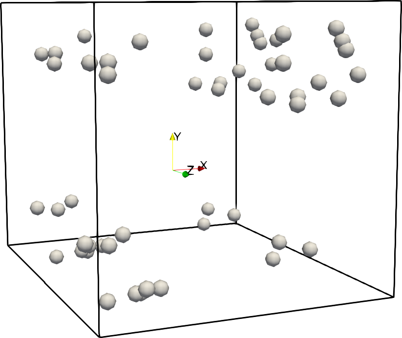
(a)

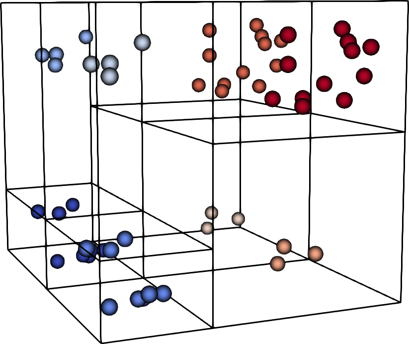
(b)

Figure 1: (a) generic distribution of particles with clustering observed in CFD-DEM simulations and (b) partitioning of particle clusters using orthogonal recursive bisection (ORB).

A generic distribution of particles that occur in a DEM simulation in a cartesian domain with clustering is shown in Fig. 1(a). A decomposition of these particles using ORB is shown in Fig. 1(b) where each subset contains the particle clusters. The explicit ORB scheme advances each of these domains separately with their local time scale to the desired global time. Therefore, domains with clustering where there are colliding particles perform multiple iterations while domains with particles that may not collide advance with larger time-steps. There are three potential advantages to this approach;

1. The use of local time-step for colliding versus non-colliding particles reduces computational cost.

2. The neighbor search is restricted to each of the sub-domains as opposed to a global $O(n^{2})$ search.

3. Advancing subsets of particles can improve temporal locality in memory as opposed to global update of all particles one after the other.

2.2 Numerical implementation

In order to achieve spatial locality of fluid and particle data, the computational domain is divided into boxes that contain the fluid and co-located particles. Message passing interface (MPI) is used for parallelization where the boxes are distributed among various MPI ranks. The distribution of boxes are obtained in way that minimizes communication distance (a space-filling curve [20] approach is used) and equalizes load (a “knapsack” [21] algorithm is applied to balance load). Each rank operate over the boxes they own and update fluid and particle fields with subsequent redistribution of ghost data. ORB strategy is used here to partition the domain into boxes that balances the number of particles. The steps in the time advancement for the traditional explicit (with global minimum particle time-step) and the explicit ORB scheme is as shown in algorithms 1 and 2, respectively. The detailed steps for the fluid update where the incompressible Navier-Stokes equations are solved, have been skipped for brevity. Readers are referred to detailed algorithms and numerical methods presented by Syamlal et al. [11].

Algorithm 1 Traditional explicit scheme

  Integrate fluid equations for time $\Delta t_{f}$ 

  Update particle drag forces 

  $\Delta t_{p}$ = global minimum particle time-step

  $t_{p}=0.0$

  while $t_{p}<\Delta t_{f}$ do

     nboxes = number of processor owned boxes

     update particle neighbor list 

     for box $i$ in nboxes do

        find collision forces for particles within box $i$ 

        use velocity-verlet time-step update for time $\Delta t_{p}$ 

     end for

     $t_{p}=t_{p}+\Delta t_{p}$ 

     redistribute ghost particles 

  end while

  Deposit particle data on grid 

  Regrid the computational domain using ORB 

Algorithm 2 explicit ORB scheme

  nsubit = number of sub-iterations

  Integrate fluid equations for time $\Delta t_{f}$ 

  Update particle drag forces 

  nboxes = number of processor owned boxes 

  $\mathrm{\Delta t_{sp}=\frac{\Delta t_{f}}{nsubit}}$ 

  initialize array “ltstep” of size nboxes 

  for it in nsubit do

     update particle neighbor list 

     for box $i$ in nboxes do

        ltstep[i]=minimum particle time-step within box $i$

     end for

     for box $i$ in nboxes do

        $t_{p}=0.0$

        while $t_{p}<\Delta t_{sp}$ do

           find collision forces for particles within box $i$ 

           use velocity-verlet time-step update for time, ltstep[i] 

           $t_{p}=t_{p}+\mathrm{ltstep[i]}$ 

        end while

     end for

     redistribute ghost particles 

  end for

  Deposit particle data on grid 

  Regrid the computational domain using ORB 

The traditional explicit method performs sub-iterations for the particle update over boxes with a global minimum time-step, while a local time-step for each box is used in the explicit ORB scheme. It should be noted that a global subcycling is also performed in the explicit ORB scheme, based on a user defined number of sub-iteration count (nsubit in Algorithm 2). This is done so as to fine-grain the update of ghost particles and their redistribution among boxes thereby reducing errors due to lag in communication. The number of sub-iterations are on the order of 5-40 for stable particle time integration; its sensitivity to errors in solution is studied in section 3 for different particle distribution scenarios. The local time-step for a particle is assigned as the collisional time scale scaled by Courant number of 0.02, when there are potential collision partners within a distance of 3 particle radii ($dt=\tau_{p}/50$) . The sub time-step, $\Delta t_{sp}$ (see Algorithm 2), obtained from the user defined sub-iteration count, is used as local time-step for particles that have no collision partners. The boxes are redefined (regrid) using ORB at the end of the fluid and particle update so as to capture new particle clusters in the subsequent time-step.

The use of local time-step for the boxes owned by processors introduces load imbalance in terms of number of time-steps performed per processor; boxes with particle clusters perform more number of time-steps compared to dilute regions. Therefore, the “knapsack” algorithm is used to rebalance loads among processors after ORB partitioning, based on local time-stepping costs associated with each box.

3 Results and discussion

The computational performance of the explicit ORB scheme is compared with the traditional explicit method in this section for various test cases in both serial and parallel execution of the algorithm. All the cases studied in this section were run on Intel Haswell 2.3 GHz processors [22] with 24 cores per node. The sensitivity of solution to the number of sub-iterations (nsubit in Algorithm 2) in the particle update for the explicit ORB scheme is studied in detail and an optimal number for different scenarios is inferred.

4 Serial cases

4.1 Homogenous cooling system (HCS)

This system consists of a cartesian domain with periodic boundaries containing particles initialized with a gaussian distribution of velocity and random position vectors. The total energy of the particles in this system decreases over time due to collisional and gas-solid drag losses. This idealized case has an analytic solution for average energy decay and such a system tends to arise in regions of gas-solid flows where there is an isotropic distribution of particles.

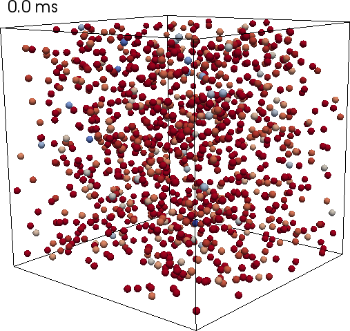
(a)

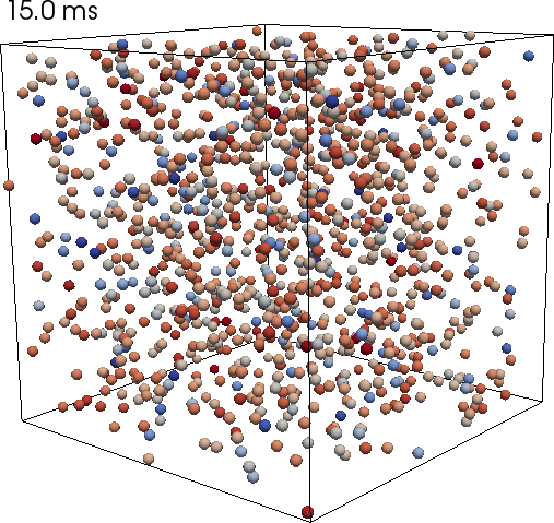
(b)

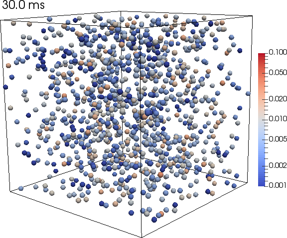
(c)

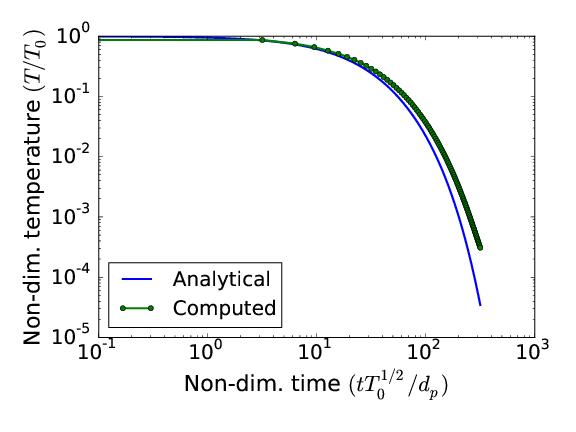
(d)

Figure 2: Snapshots of particle specific kinetic energy ($k=\frac{1}{2}|\mathbf{v}|^{2}$) in $\mathrm{m^{2}/s^{2}}$ for the HCS simulation at (a) 0 , (b) 15 and (c) 30 ms, respectively. (d) shows the simulated and analytic solutions for particle averaged temperature ($T=\frac{1}{3}\overline{\mathrm{v}^{2}}$) decay as a function of time. Here, $T$ is normalized by the initial temperature, $T_{0}$ and time is normalized by $\frac{d_{p}}{\sqrt{T_{0}}}$ where $d_{p}$ is the particle diameter.

Simulation parmeters	Value
Particle diameter ($d_{p}$)	$\mathrm{100}~{}\mu m$
Particle density ($\rho_{p}$)	$\mathrm{1000~{}kg/m^{3}}$
Gas density ($\rho_{g}$)	$\mathrm{1~{}kg/m^{3}}$
Gas viscosity ($\mu_{g}$)	$\mathrm{2\times 10^{-5}~{}Pa~{}sec}$
Collisional spring constant ($k$)	$\mathrm{10~{}N/m}$
Restitution coefficient ($e$)	0.8
Fluid time-step ($\Delta t_{f}$)	0.0001 sec
Drag model	BVK model [23]

Table 1: Simulation parameters for the homogenous cooling system case

Fig. 2(a), (b) and (c) show snapshots of particles colored by their kinetic energy at 0, 15 and 30 ms for a typical HCS simulation performed in a cubical domain of size 4 mm with 1222 particles, indicating the decay of energy over time. The mesh consists of 8000 cells with 20 cells along each coordinate direction. The material parameters for the gas and solid phase are described in Table 1.

Fig. 2(d) shows the comparison between the computed and analytic solutions for the temperature ($T=\frac{1}{3}\overline{\mathrm{v}^{2}}$) decay as predicted by the Haff’s law [24, 25], indicating reasonable agreement. Slight deviations are observed due to the idealized assumptions (such as constant collision cross-section) used in the analytic derivation of Haff’s law.

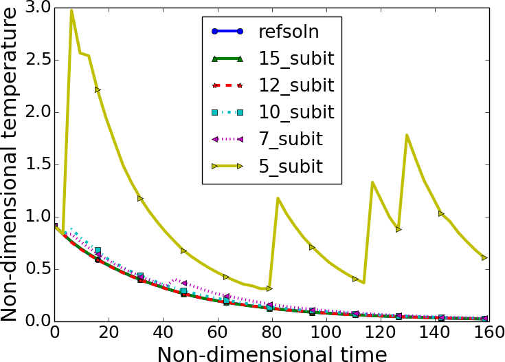
(a)

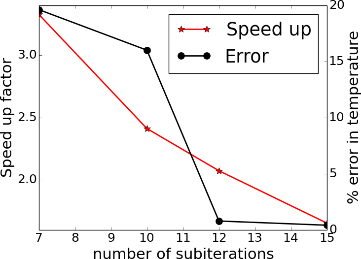
(b)

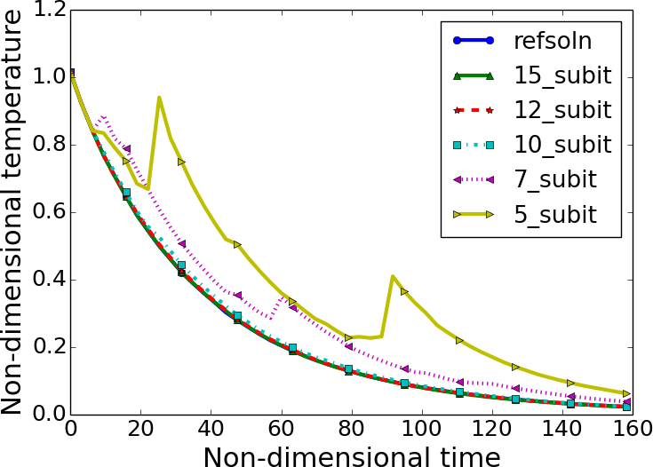
(c)

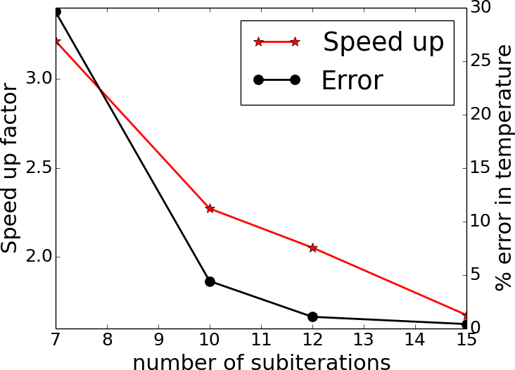
(d)

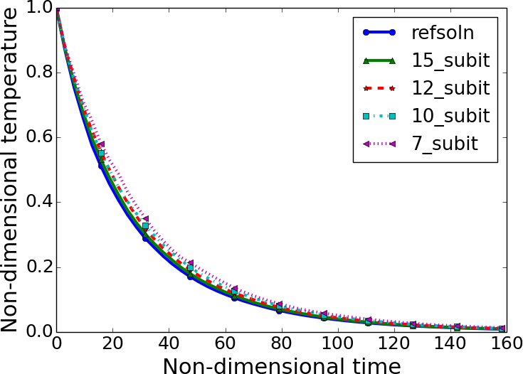
(e)

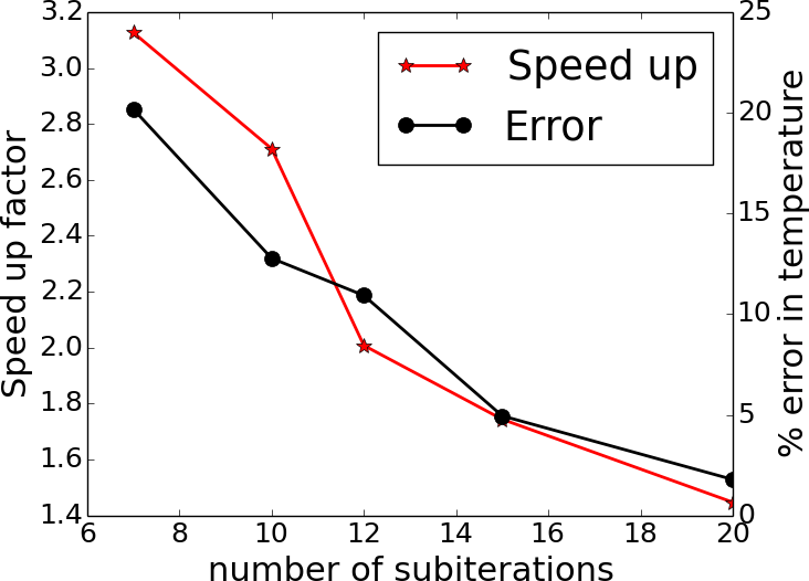
(f)

Figure 3: Computed solution of temperature decay using the explicit ORB method with varying number of sub-iterations for (a) 100, (c) 200 and (e) 1222 particles, respectively. Figures (b), (d) and (f) show the variation of error in non-dimensional temperature between the explicit ORB and the traditional explicit method along with the speed-up achieved for varying number of sub-iteration counts.

Fig. 3 compares the non-dimensional temperature decay predicted by the traditional explicit and the explicit ORB scheme for varying number of particle and sub-iteration counts. The traditional explicit scheme solution is assumed to be the reference and an average temperature error is obtained for the explicit ORB method for varying number of sub-iteration counts. The error is further normalized by the time-averaged temperature so as to quantify the fractional deviation in the solution.

Fig. 3(a), (c) and (e) show temperature decay solutions for varying number of particles in the domain from 100 to 1222 particles. 4 ORB levels (16 leaves) are used for the lower particle count cases (100 and 200) while 6 levels (64 leaves) are used for the simulation with 1222 particles. Large deviations from the reference solution is observed for lower number of sub-iterations in the explicit ORB scheme. The larger the sub time-step, the greater is the chance of missing collisions thereby increasing the error. Fig. 3(b), (d) and (f) show the variation of the speed-up factor and the error as a function of number of sub-iterations. As the number of sub-iterations is increased, the explicit ORB method tends towards the traditional explicit scheme and its performance is reduced while lower number of sub-iterations result in greater error in the solution. Nonetheless, a nominal speed-up factor of 2X is obtained with 10-15 sub-iterations for all the 3 cases, with errors in the range of 1-5% with respect to the traditional explicit method.

4.2 Particle settling problem

The settling of particles due to gravity in a cartesian domain is studied in this section. The particle distribution here transitions from being uniformly distributed to a settled bed that is densely packed, thereby testing the performance and accuracy of the explicit ORB scheme with time varying particle densities.

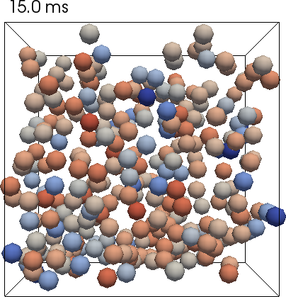
(a)

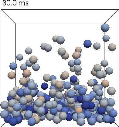
(b)

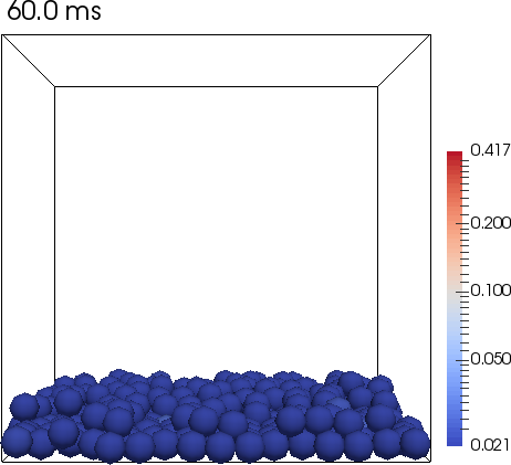
(c)

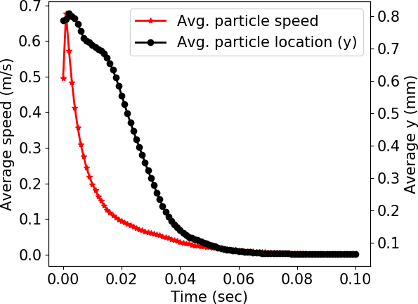
(d)

Figure 4: Snapshots of particle speed ($|\mathbf{v}|$) in $\mathrm{m/s}$ for the particle settling simulation at (a) 15 , (b) 30 and (c) 60 ms, respectively. (d) shows the particle averaged position along the direction of gravity (y) and speed vs time.

Fig. 4 illustrates the physics of the settling simulation through time snapshots and particle averaged parameters. This simulation consists of 300 particles in a cubical box, 1.5 mm in size. The mesh consists of 1000 cells with 10 cells along each coordinate direction. The material properties used in this simulation is the same as the HCS case, as described in Table 1. Gravity is assumed to be along the y coordinate direction (top to bottom). The particles that are uniformly distributed initially, settle and lose their gravitational potential energy through drag, inter-particle and wall collisions. Fig. 4(a) to (c) show particle distribution colored by their speeds from 15 to 60 ms; the particle kinetic energy is observed to dissipate completely at the end of 60 ms. Fig. 4(d) shows the average particle speed and position along the y direction; the particle speeds are observed to rise initially during free fall and assymptotes to 0 after longer time periods.

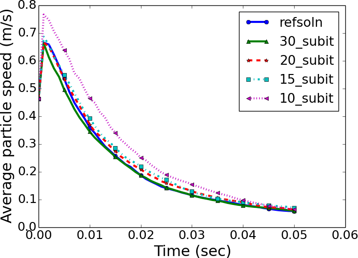
(a)

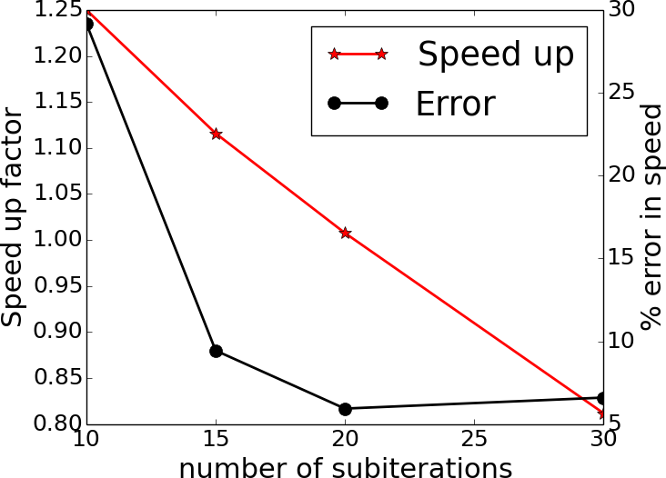
(b)

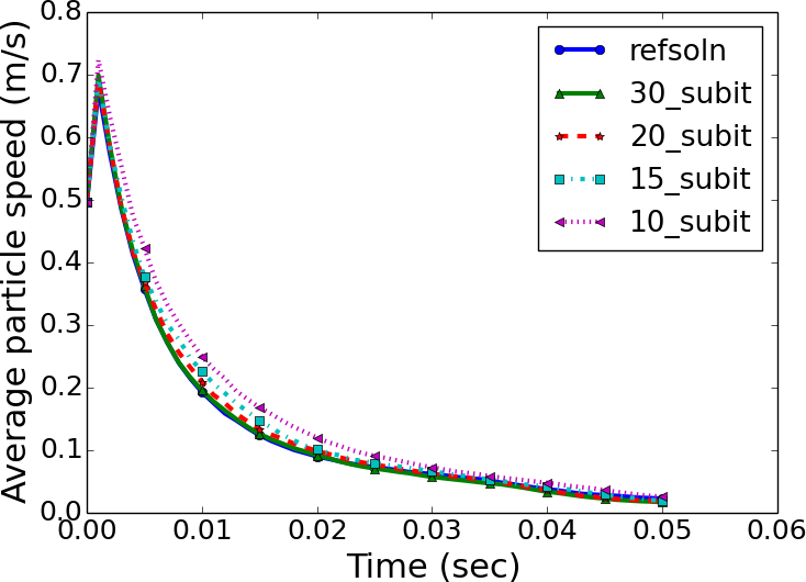
(c)

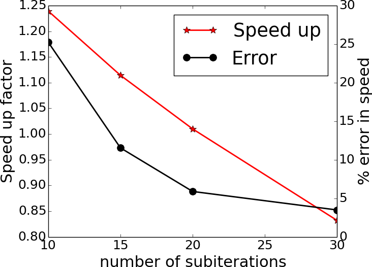
(d)

Figure 5: Computed solution of average particle speed using the traditional explicit and explicit ORB method with varying number of sub-iterations for (a) 100 and (c) 300, respectively. (b) and (d) show the variation of error in particle averaged speed between the explicit ORB and the traditional explicit method along with the speed-up achieved for varying number of sub-iteration counts.

Fig. 5 shows the effect of sub-iteration count in the explicit ORB scheme on the solution accuracy. Fig. 5(a) and (c) show the average particle speed as a function of time for simulations with 100 and 300 particles, respectively, for varying number of sub-iteration counts. These simulations are performed with 4 ORB levels (16 leaves).

A similar trend with respect to the HCS test case is observed; larger number of sub-iterations reduce the error in solution as shown in Fig. 5(b) and (d), respectively. The error in the explicit ORB solution (Fig. 5(b) and (d)) is computed based on the average particle speed variation with respect to the reference traditional explicit scheme solution. The speed-up factor achieved with the use of explicit ORB scheme is lower in this case due to the highly collisional distribution of particles. There is no speed-up observed using the explicit ORB scheme for maintaining solution errors within 1-5%.

The explicit ORB scheme thus performs better when there are dilute regions in the domain. The settling of particles in this problem rapidly transitions the system into a dense distribution, thereby enforcing small particle time-steps in all boxes. The traditional explicit scheme is recovered for dense distributions where a global small time-step is the same as the local time-step.

5 Parallel cases

5.1 Riser flow

This test case is representative of industrial systems such as circulating fluidized bed (CFB) riser reactors [26] that are applied to catalytic cracking and combustion. This simulation consists of a rectangular column with a 6 mm x 6 mm cross section and a height of 1 cm, with 14,000 particles seeded uniformly in the domain with periodic boundary conditions at all faces. A constant pressure gradient of 2 Pa along the axial direction is imposed. Simulations are performed on 64 MPI ranks with 7 ORB levels (maximum of 128 leaves) on a mesh of 51,200 cells (32 x 50 x 32 grid). The material properties from Table 1 along with the Koch-Hill drag model [27] is used in these simulations.

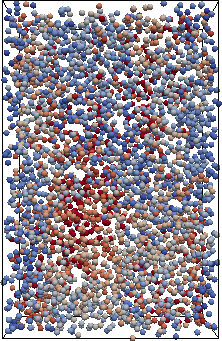
(a)

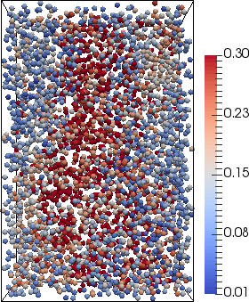
(b)

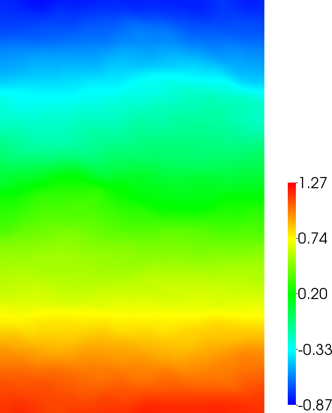
(c)

Figure 6: Snapshots of particle distribution colored by their speed in m/s for the riser flow simulation at (a) 300 ms and (b) 400 ms, respectively. (c) shows the distribution of pressure (Pa) in the domain at t=400 ms.

Fig. 6 shows the snapshots of particle distribution and fluid pressure; the favorable bottom-to-top pressure gradient facilitates movement of particles predominantly along the axis. The particles are recycled back into the domain via the periodic boundaries and are steadily accelerated due to the constant pressure gradient.

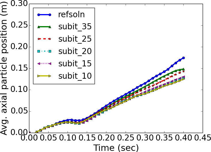
(a)

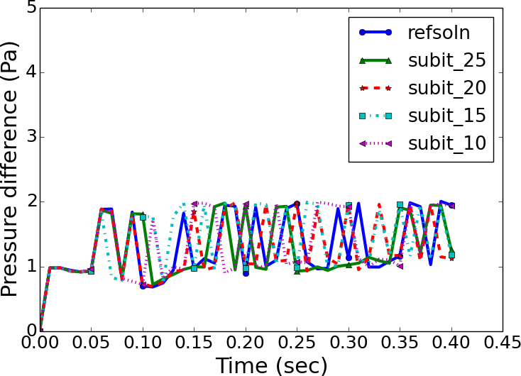
(b)

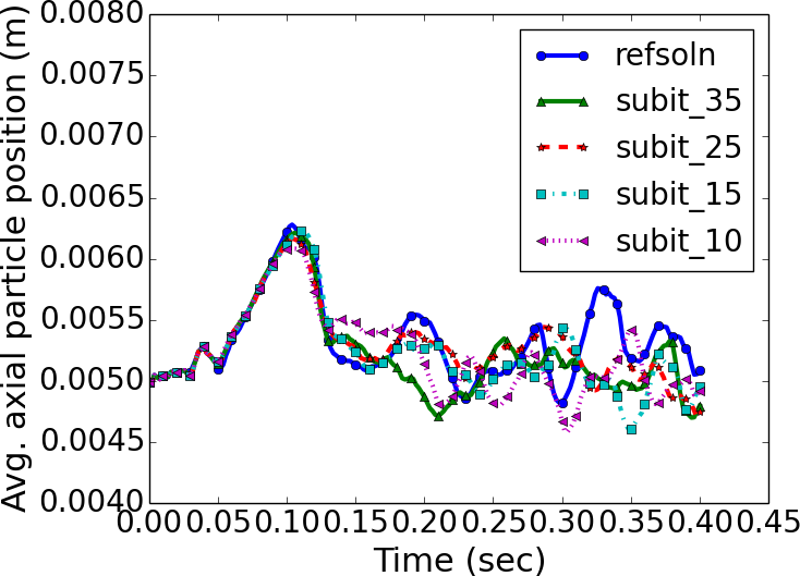
(c)

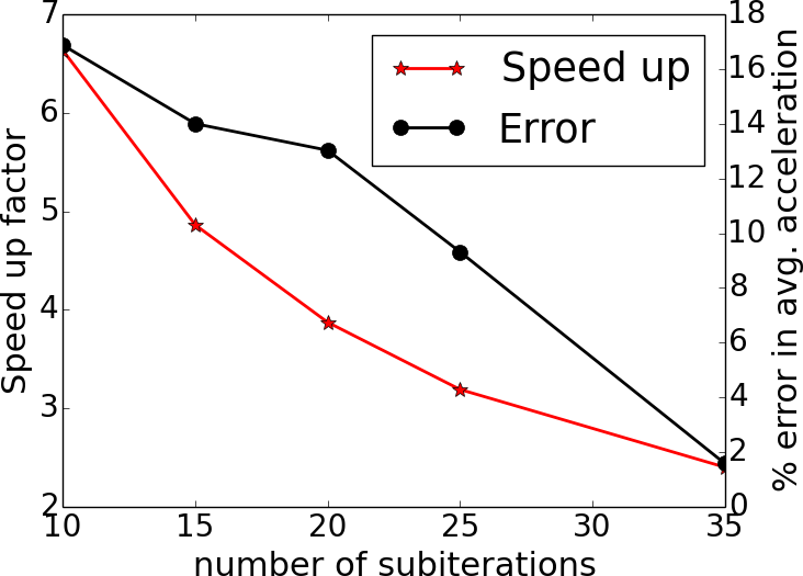
(d)

Figure 7: (a) particle averaged speed along the axial direction, (b) pressure difference between riser top and bottom and (c) is the particle averaged position along the axis as a function of time and varying sub-iteration counts. (d) plots the variation of speed-up and error in particle averaged acceleration with respect to the traditional explicit method for varying number of sub-iterations in the explicit ORB scheme.

The average particle speed along the axial direction as a function of time is shown in Fig. 7(a) for the reference traditional explicit time-stepping as well as the explicit ORB scheme with varying number of sub-iterations. The average speeds are observed to approach a constant slope with respect to time indicating a steady-state acceleration. There is reasonable agreement among the explicit ORB cases with higher error for lower number of sub-iteration counts. Fig. 7(b) shows the pressure difference between the top and bottom of the column as a function of time for this case. This parameter approaches a fluctuating steady-state within 0.15 seconds; the explicit ORB scheme is able to achieve the averaged steady-state value for all sub-iteration counts. Fig. 7(c) shows the average particle position along the axial direction as a function of time. A fluctuating steady-state about the middle of the column (0.005 m from the bottom) is attained for all the cases with reasonable agreement. Fig. 7(d) shows the sensitivity of sub-iteration count on solution accuracy and the speed-up obtained using the explicit ORB method. The steady-state acceleration is chosen as the parameter of interest for computing errors with respect to the reference traditional explicit method. The errors are within 1-2% for about 35 sub-iterations along with a 2X speed-up using the explicit ORB scheme.

5.2 Fluidized bed

This case consists of a rectangular column with a 1.6 mm x 1.6 mm cross section and a height of 1 cm, with 10,000 particles seeded initially close to the bottom of the column, on a mesh of 51,200 cells (32 x 50 x 32 grid). A constant velocity inflow boundary condition is applied to the bottom face with a fixed normal gas velocity of 1.5 cm/s; the lateral surfaces are assumed to be no-slip walls and pressure outflow boundary condition is used at the top. This simulation uses the same material properties as in the riser case (section 5.1) and is perfomed using 16 MPI ranks with 6 ORB levels (64 leaves).

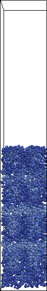
(a)

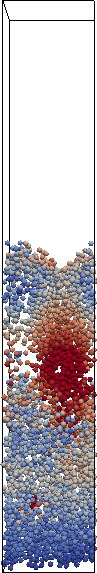
(b)

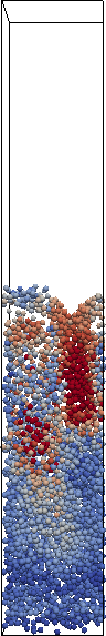
(c)

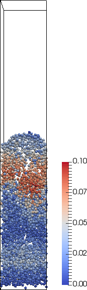
(d)

Figure 8: Snapshots of particle distribution colored by their speed in m/s for the fluidized bed simulation at (a) 0, (b) 100, (c) 200 and (d) 400 ms, respectively.

Fig. 8 shows the snapshots of particle distribution in the domain at four time points between 0 and 400 ms, indicating top-to-bottom mixing, typically seen in fluidized bed reactors.

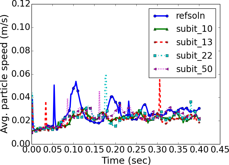
(a)

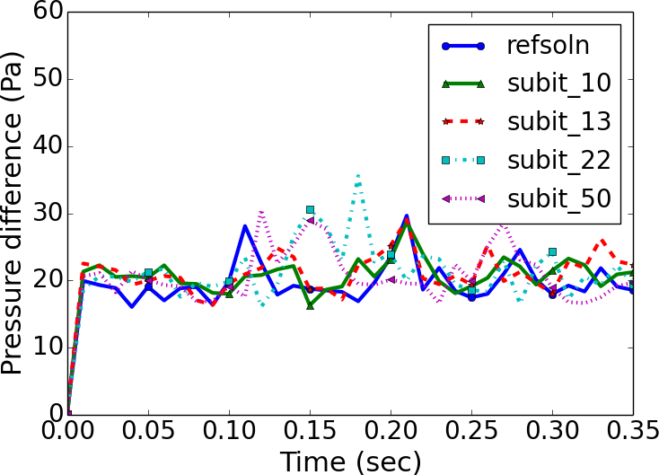
(b)

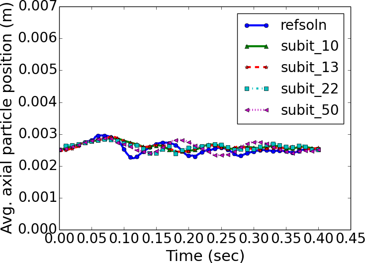
(c)

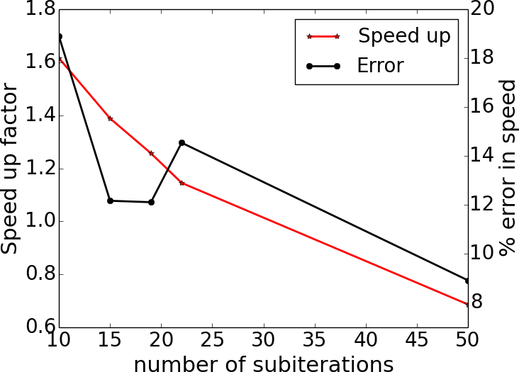
(d)

Figure 9: (a) particle averaged speed, (b) top to bottom pressure difference and (c) particle averaged axial position in the fluidized bed as a function of time for the traditional explicit and the explicit ORB scheme with varying sub-iteration counts. (d) is the variation of speed-up and error in steady-state particle averaged speed solution for varying number of sub-iterations.

Fig. 9 quantifies the accuracy and performance of the explicit ORB scheme for varying number of sub-iteration counts. The fluidized bed is a chaotic system with dense particle distributions; a fluctuating steady-state for the particle speeds is achieved in about 100 ms (Fig. 9(a)) with intermittent peaks in average particle speeds over time. The explicit ORB scheme solutions show comparable trends with respect to the traditional explicit scheme and approach similar averaged particle speeds at steady-state. Fig. 9(b) shows the variation of pressure difference between the top and bottom of the column; a fluctuating steady-state is attained within 50 ms. All of the explicit ORB scheme cases exhibit the same trend as the reference explicit solution with the nominally similar average pressure drop at steady-state. The variation of average axial particle position with time is shown Fig. 9(c) indicating agreement among the explicit ORB scheme cases with respect to the reference solution.

Fig. 9(d) shows the variation of speed-up and error in steady-state time-averaged particle speed for varying sub-iteration counts in the explicit ORB scheme. A speed-up of 1.1-1.3X is seen for 12-20 sub-iteration counts with solution errors on the order of 12-14%. The number of sub-iterations needs to be around 50 to bound the errors within 10% for which no speed-up is observed.

This case reinforces the need for dilute regions in the problem for optimal performance of the explicit ORB scheme. The dense particle distributions in this problem will require the global resolution of collisional time scales among all particles thereby negating any performance improvements from the explicit ORB scheme.

6 Conclusions and future work

An adaptive timestepping method is developed to speed up CFD-DEM simulations using an orthogonal recursive bisection based approach. This algorithm was implemented in a parallel CFD-DEM solver and its performance was compared against the baseline explicit scheme with a global time step. Four different test cases with dilute and dense particle distributions were studied to quantify the efficacy of this method. The dilute cases (homogenous cooling system and riser flow) showed a 2-3X speed-up relative to baseline explicit scheme, while maintaining minimal solution errors. The dense cases on the other hand (settling and fluidized bed) showed minimal speed-up to maintain low solution errors. The current method provides a means of setting the timestep appropriately on a particle cluster basis, but caution should be used away from collisions to ensure that accuracy requirements (e.g., based on path line integration considerations) are still met.

Other bisection strategies such as k-means clustering that respect clustering and probable collision partners will be studied in the context of relatively denser distributions. A relative distance based time step estimate instead of a bimodal distribution used in this work, will be considered to prevent collision misses in dense systems.

References

References

- [1] G. G. Joseph, J. Leboreiro, C. M. Hrenya, A. R. Stevens, Experimental segregation profiles in bubbling gas-fluidized beds, AIChE journal 53 (11) (2007) 2804–2813.
- [2] Y. Tsuji, T. Kawaguchi, T. Tanaka, Discrete particle simulation of two-dimensional fluidized bed, Powder technology 77 (1) (1993) 79–87.
- [3] X. Lan, C. Xu, G. Wang, L. Wu, J. Gao, Cfd modeling of gas–solid flow and cracking reaction in two-stage riser fcc reactors, Chemical Engineering Science 64 (17) (2009) 3847–3858.
- [4] A. Dutta, D. Constales, G. J. Heynderickx, Applying the direct quadrature method of moments to improve multiphase fcc riser reactor simulation, Chemical engineering science 83 (2012) 93–109.
- [5] R. Kolakaluri, S. Subramaniam, M. V. Panchagnula, Trends in multiphase modeling and simulation of sprays, International Journal of Spray and Combustion Dynamics 6 (4) (2014) 317–356.
- [6] J. Capecelatro, P. Pepiot, O. Desjardins, Numerical investigation and modeling of reacting gas-solid flows in the presence of clusters, Chemical Engineering Science 122 (2015) 403–415.
- [7] Y. Tsuji, T. Tanaka, S. Yonemura, Cluster patterns in circulating fluidized beds predicted by numerical simulation (discrete particle model versus two-fluid model), Powder Technology 95 (3) (1998) 254–264.
- [8] H. Kruggel-Emden, M. Sturm, S. Wirtz, V. Scherer, Selection of an appropriate time integration scheme for the discrete element method (dem), Computers & Chemical Engineering 32 (10) (2008) 2263–2279.
- [9] E. Rougier, A. Munjiza, N. John, Numerical comparison of some explicit time integration schemes used in dem, fem/dem and molecular dynamics, International journal for numerical methods in engineering 61 (6) (2004) 856–879.
- [10] K. Samiei, Assessment of implicit and explicit algorithms in numerical simulation of granular matter, Ph.D. thesis, University of Luxembourg, Luxembourg, Luxembourg (2012).
- [11] M. Syamlal, W. Rogers, T. J. O’Brien, Mfix documentation: Theory guide, National Energy Technology Laboratory, Department of Energy, Technical Note DOE/METC-95/1013 and NTIS/DE95000031.
- [12] A. S. Almgren, V. E. Beckner, J. B. Bell, M. S. Day, L. H. Howell, C. C. Joggerst, M. J. Lijewski, A. Nonaka, M. Singer, M. Zingale, CASTRO: A New Compressible Astrophysical Solver. I. Hydrodynamics and Self-gravity, Astrophysical Journal 715 (2010) 1221–1238. arXiv:1005.0114, doi:10.1088/0004-637X/715/2/1221.
- [13] R. Garg, J. Galvin, T. Li, S. Pannala, Documentation of open-source mfix–dem software for gas–solids flows, From URL https://mfix. netl. doe. gov/documentation/dem_doc_2012-1. pdf.(Accessed: 31 March 2014).
- [14] L. Verlet, Computer” experiments” on classical fluids. i. thermodynamical properties of lennard-jones molecules, Physical review 159 (1) (1967) 98.
- [15] C. O’Sullivan, J. D. Bray, Selecting a suitable time step for discrete element simulations that use the central difference time integration scheme, Engineering Computations 21 (2/3/4) (2004) 278–303.
- [16] M. J. Berger, S. H. Bokhari, A partitioning strategy for nonuniform problems on multiprocessors, IEEE Transactions on Computers (5) (1987) 570–580.
- [17] S. Popov, J. Günther, H.-P. Seidel, P. Slusallek, Stackless kd-tree traversal for high performance gpu ray tracing, in: Computer Graphics Forum, Vol. 26, Wiley Online Library, 2007, pp. 415–424.
- [18] T. Kanungo, D. M. Mount, N. S. Netanyahu, C. D. Piatko, R. Silverman, A. Y. Wu, An efficient k-means clustering algorithm: Analysis and implementation, IEEE transactions on pattern analysis and machine intelligence 24 (7) (2002) 881–892.
- [19] R. L. Graham, P. Hell, On the history of the minimum spanning tree problem, Annals of the History of Computing 7 (1) (1985) 43–57.
- [20] G. Peano, Sur une courbe, qui remplit toute une aire plane, Mathematische Annalen 36 (1) (1890) 157–160.
- [21] C. A. Rendleman, V. E. Beckner, M. Lijewski, W. Crutchfield, J. B. Bell, Parallelization of structured, hierarchical adaptive mesh refinement algorithms, Computing and Visualization in Science 3 (3) (2000) 147–157.
- [22] Products formerly haswell., http://ark.intel.com/products/codename/42174/Haswell.
- [23] R. Beetstra, M. A. van der Hoef, J. Kuipers, Drag force of intermediate reynolds number flow past mono-and bidisperse arrays of spheres, AIChE journal 53 (2) (2007) 489–501.
- [24] P. Haff, Grain flow as a fluid-mechanical phenomenon, Journal of Fluid Mechanics 134 (1983) 401–430.
- [25] W. Fullmer, C. Hrenya, The homogeneous cooling state as a verification test for kinetic-theory-based continuum models of gas-solid flows, Journal of Verification, Validation and Uncertainty Quantification.
- [26] H. Zhang, W.-X. Huang, J.-X. Zhu, Gas-solids flow behavior: Cfb riser vs. downer, AIChE Journal 47 (9) (2001) 2000–2011.
- [27] R. J. Hill, D. L. Koch, A. J. Ladd, The first effects of fluid inertia on flows in ordered and random arrays of spheres, Journal of Fluid Mechanics 448 (2001) 213–241.