Near-Linear Time Local Polynomial Nonparametric Estimation

Near-Linear Time Local Polynomial Nonparametric Estimation with Box Kernels

Yining Wang Warrington College of Business, University of Florida, Gainesville, FL 32611, USA. Yi Wu Institute of Interdisciplinary Information Sciences, Tsinghua University, Beijing, 100084, China. Simon S. Du Paul G. Allen School of Computer Science and Engineering, University of Washington, WA 98195, USA.

Local polynomial regression (Fan and Gijbels 1996) is an important class of methods for nonparametric density estimation and regression problems. However, straightforward implementation of local polynomial regression has quadratic time complexity which hinders its applicability in large-scale data analysis. In this paper, we significantly accelerate the computation of local polynomial estimates by novel applications of multi-dimensional binary indexed trees (Fenwick 1994). Both time and space complexity of our proposed algorithm is nearly linear in the number of input data points. Simulation results confirm the efficiency and effectiveness of our proposed approach.

local polynomial regression, nonparametric density estimation, binary indexed trees, hashing

1 Introduction

Big data analytics has become essential for modern operations research and operations management applications (Choi et al. 2018, Hazen et al. 2018, Mišić and Perakis 2019). Statistics methods, such as nonparametric density and function estimation (Larry 2006, Tsybakov 2009, Friedman et al. 2001), play important roles in the prediction of econometric trends like loan management and market profit prediction (Györfi et al. 2006), as well as exploratory data analysis as preliminary steps to operations management problems, such as the understanding and estimation of customers’ demand or preferences in revenue management applications. Naturally, big data scenarios pose unique challenges from computing aspects, as many classical statistical computational routines (especially nonparametric statistical methods) are computationally heavy and not scalable to large amounts of data.

The focus of this paper is on nonparametric density estimation and regression problems. Let $\mathcal{X}\subseteq\mathbb{R}^{d}$ be a compact domain in $\mathbb{R}^{d}$, which is conventionally taken to be the unit cube $[0,1]^{d}$ for convenience. In the nonparametric density estimation problem, $n$ independent samples $X_{1},\cdots,X_{n}\in\mathcal{X}$ are obtained as

$$X_{1},\cdots,X_{n}\;\overset{i.i.d.}{\sim}\;f_{0},$$ (1)

where $f_{0}$ is the density of an unknown distribution $P_{0}$ supported on $\mathcal{X}$. In the nonparametric regression problem, on each of $n$ “design points” $X_{1},\cdots,X_{n}\in\mathcal{X}$ a “response” or “measurement” $Y_{i}$ is obtained according to the model

$$Y_{i}=m_{0}(X_{i})+\xi_{i},\;\;\;\;\;i=1,\cdots n,$$ (2)

where $m_{0}:\mathcal{X}\to\mathbb{R}$ is an unknown regression model of interest, and $\{\xi_{i}\}$ are independent sub-Gaussian noise variables satisfying $\mathbb{E}[\xi_{i}|X_{i}]=0$. The objective in both nonparametric estimation problems is to construct estimates $\widehat{f}_{n}$ or $\widehat{m}_{n}$ such that the mean-square error (MSE)

$$\int_{\mathcal{X}}\big{|}\widehat{f}_{n}(x)-f_{0}(x)\big{|}^{2}\mathrm{d}x\;\;\text{or}\;\;\int_{\mathcal{X}}\big{|}\widehat{m}_{n}(x)-m_{0}(x)\big{|}^{2}\mathrm{d}x$$

is minimized.

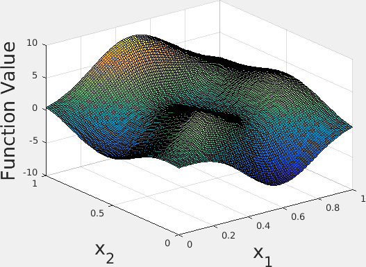
(a) The ground truth function.

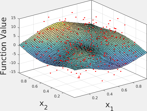
(b) Naive impl., $n=4000$, 75 secs

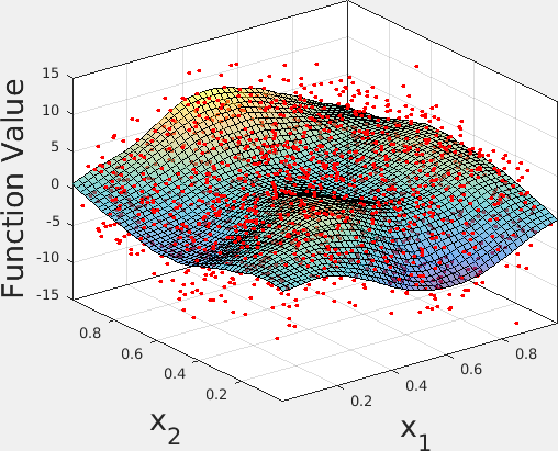
(c) Fast impl., $n=16000$, 10 secs

Figure 1: Illustration of local polynomial regression with naive and fast implementation for fitting a two dimensional smooth function $f(x,y)=3(1-x)^{2}e^{-x^{2}-(y+1)^{2}}-10(0.2x-x^{3}-y^{5})e^{-x^{2}-y^{2}}-e^{-(x+1)^{2}-y^{2}}/3$. Red points are observations (training points), down sampled $10\times$ for better visualization. The number of testing points is large ($\sim 1,000,000$), as reconstruction of the entire function is desired. Under such settings, the naive implementation (middle panel) takes $75$ secs to process $n=4000$ observations (training points), while our fast implementation (Algorithm 1, right panel) only takes $10$ secs to process $n=16000$ observations. As a result, there is a visible difference between the fitted curves under the naive and the fast implementation, because the naive implementation can only process a small number of observations under given time budget and therefore needs to significantly “over-smooth” the data, leading to inaccurate function reconstruction. Indeed, the mean-square errors of the naive and fast implementation are $9\times 10^{-3}$ and $2\times 10^{-3}$ respectively, which is a near $5\times$ gap.

The nonparametric density estimation and regression problems have a long history of study, dating back to the 1920s (Whittaker 1922). A large family of methods have been developed and their properties analyzed, including kernel smoothing (Friedman et al. 2001, Györfi et al. 2006), spline smoothing (Reinsch 1967, Geer 2000, Green and Silverman 1993), wavelet smoothing (Donoho et al. 1998, Donoho and Johnstone 1994, Härdle et al. 2012) and local polynomial regression (Fan and Gijbels 1992, Fan 1993, Fan and Gijbels 1996).

In this paper, we concentrate on the local polynomial regression method introduced in (Fan and Gijbels 1992, Fan 1993, Fan and Gijbels 1996). Compared to its competitors, local polynomial regression has the benefits of being adaptive to non-uniform design densities and regression functions of unbounded values (Hastie and Loader 1993). In Sec. 2 we give a succinct description of these methods and also summarize some of their basic properties.

While the statistical properties of local polynomial regression are well understood, computational efficiency has been less studied. In particular, straightforward implementation of local polynomial regression typically has quadratic time complexity $O(sn)$ to calculate $\widehat{f}_{n}(z_{i})$ or $\widehat{m}_{n}(z_{i})$ on $s$ “testing points” $z_{1},\cdots,z_{s}\in\mathcal{X}$, which is prohibitively slow for analysis of large data sets. We give an illustrative example in Figure 1, which shows that the computational bottleneck of the naive implementation of local polynomial regression significantly restricts the number of observations (training points) it processes under given time budget, leading to inaccurate function estimates.

The apparent difficulties of computationally efficient local polynomial regresstion motivate the following question:

Question 1.1

Given $n$ training data points $\{(X_{i},Y_{i})\}_{i=1}^{n}$ and $s$ testing points $z_{1},\cdots,z_{s}\in\mathcal{X}$, can we compute local polynomial estimates $\widehat{f}_{n}(z_{1}),\cdots,\widehat{f}_{n}(z_{s})$ or $\widehat{m}_{n}(z_{1}),\cdots,\widehat{m}_{n}(z_{s})$ in $O((n+s)\mathrm{poly}\log n)$ time?

Essentially, Question 1.1 concerns estimation algorithms whose time complexity is nearly linear in the total number of training and testing points $n+s$, apart from possible poly-logarithmic factors. On the other hand, a linear dependency on $n+s$ is clearly necessary as the number of inputs is already on the order of $n+s$.

We give an affirmative answer to Question 1.1 in this paper by accelerating local polynomial regression using efficient data structures. In particular, applying a multi-dimensional extension of binary indexed trees (Fenwick 1994) we are able to reduce the computation time on each testing point from $O(n)$ to $O(\log^{d}n)$. Furthermore, to avoid space complexity growing exponentially with dimension $d$, we consider a lazy allocation strategy that allocates memory on the fly with the help of a Hash table, which achieves near-linear space complexity. Our computations of all local polynomial estimates are exact, and therefore all statistical properties of local polynomial regression are automatically preserved.

Finally, we remark that certain existing nonparametric estimation methods can also achieve near-linear time complexity, such as the B-spline (De Boor 1978) and/or falling factorial basis (Wang et al. 2014) construction in smoothing splines and block thresholding of wavelet coefficients (Cai 1999). However, both smoothing spline and wavelet thresholding (shrinkage) methods become very complicated for multi-dimensional and non-uniformly spaced data points. For example, the extension of smoothing splines to higher dimension requires complicated constructions of the “thin-plate” splines, and in the case of wavelet smoothing the basis functions are complicated and difficult to compute when design points are not evenly spaced. On the other hand, the local polynomial regression method easily handles both cases of multi-dimensionality and unevenly spaced design points without much additional complexity.

2 Local polynomial regression

In this section we give a succinct description of local polynomial regression (Fan and Gijbels 1996) in the context of nonparametric estimation problems, with high-level summarization of its properties.

Let $k\in\mathbb{N}$ be the desired polynomial degree used in estimation. Practical choices of $k$ are small non-negative integers, such as $k=0$ (local mean averaging), $k=1$ (local linear regression) and $k=2$ (local quadratic regression). For any $z\in\mathbb{R}^{d}$, define the polynomial mapping $\psi_{z}:\mathbb{R}^{d}\to\mathbb{R}^{D}$, $D=1+d+\cdots+d^{k}$ as

$$\psi_{z}(x) :=[1,x_{1}-z_{1},\cdots,x_{d}-z_{d},(x_{1}-z_{1})^{2},(x_{1}-z_{1})(x_{2}-z_{2}),\cdots,(x_{d}-z_{d})^{2},$$

$$\cdots,(x_{1}-z_{1})^{k},\cdots,(x_{d}-z_{d})^{k}].$$

At a higher level, the polynomial mapping $\psi_{x}(\cdot)$ is an expansion of basis of degree-$k$ polynomials on $\mathbb{R}^{d}$, appropriately offset so that $\psi_{z}(z)=[1,0,\cdots,0]$. As we shall see immediately, the mapping $\psi_{z}$ plays a fundamental role in local polynomial regression methods.

We first consider the regression problem $Y_{i}=m_{0}(X_{i})+\xi_{i}$. We start by introducing the concepts of kernel functions and bandwidths, which are crucial to almost every nonparametric estimation method:

1. A kernel function $K:\mathbb{R}\to\mathbb{R}$ that satisfies constraints $\int_{-\infty}^{\infty}K(u)\mathrm{d}u=1$, $\int_{-\infty}^{\infty}K(u)u\mathrm{d}u=0$ and $\int_{-\infty}^{\infty}K^{2}(u)\mathrm{d}u<\infty$ is used to “average” neighboring data points in a certain manner. Common kernel functions include the box kernel $K(u)=\mathbb{I}[|u|\leq 1/2]$, the Gaussian kernel $K(u)=\frac{1}{\sqrt{2\pi}}e^{-u^{2}/2}$ and the Epanechnikov kernel $K(u)=\frac{3}{4\sqrt{5}}\max(0,1-u^{2}/5)$.

2. A bandwidth parameter $h>0$ is used to control the size of the “neighborhood” of a certain test point $z\in\mathcal{X}$ in which training points are incorporated and smoothed. A small bandwidth $h$ will have fewer effective training points rendering the variance of the resulting estimate large, while a large bandwidth $h$ tends to “over-smooth” the unknown function over a large domain and therefore leading to larger estimation bias.

To estimate the value of the unknown regression function $m_{0}$ at a specific testing point $z$, first solve a weighted least-squares problem

$$\widehat{\theta}_{n}=\arg\min_{\theta\in\mathbb{R}^{D}}\sum_{i=1}^{n}{(Y_{i}-\theta^{\top}\psi_{z}(X_{i}))^{2}K\left(\frac{\|z-X_{i}\|_{\infty}}{h}\right)}$$ (3)

where $\|z-X_{i}\|_{\infty}=\max_{1\leq j\leq d}|z_{j}-X_{ij}|$. Afterwards, $\widehat{m}_{n}(z)$ is taken to be $\widehat{\theta}_{n}^{\top}\psi_{z}(z)$, which corresponds to the first component of $\widehat{\theta}_{n}$.

Example 2.1

When $K(\cdot)$ is taken to be the box kernel $K(u)=\mathbb{I}[|u|\leq 1/2]$, Eq. (3) can be re-formulated as

$$\widehat{g}_{n}=\arg\min_{g\in\mathcal{P}_{k}}\sum_{X_{i}\in B_{h}(z)}(Y_{i}-g(X_{i}))^{2}$$

where $\mathcal{P}_{k}$ is the class of all degree-$k$ polynomials on $\mathbb{R}^{d}$ and $B_{h}(z)=\{u\in\mathcal{X}:\|u-z\|_{\infty}\leq h/2\}$ denotes the neighborhood of $z$ with radius $h$. The re-formulation of $\widehat{g}_{n}$ is a clear interpretation of the polynomial fitting (in $\mathcal{P}_{k}$) and the local properties (in $B_{h}(z)$).

The density estimation problem is slightly more involved than local polynomial regression. Here we adopt the approach in (Cattaneo et al. 2017) by re-casting the density estimation problem as a regression problem. For every $X_{i}\in\mathcal{X}$ define empirical cumulative density function (CDF)

$$\widehat{F}(X_{i}):=\frac{1}{n}\sum_{j=1}^{n}\mathbb{I}\left[X_{j1}\leq X_{i1},\cdots,X_{jd}\leq X_{id}\right]$$ (4)

that approximates the true CDF $F(X_{i})=\int_{\mathcal{X}}\mathbb{I}[u_{1}\leq X_{i1},\cdots,u_{d}\leq X_{id}]f_{0}(u)\mathrm{d}u$. Afterwards, a local polynomial fit of $\widehat{F}$ is computed as

$$\widehat{\beta}_{n}=\arg\min_{\beta\in\mathbb{R}^{D}}\sum_{i=1}^{n}{(\widehat{F}(X_{i})-\theta^{\top}\psi_{z}(X_{i}))^{2}K\left(\frac{\|z-X_{i}\|_{\infty}}{h}\right)}.$$

Because $f_{0}=\partial^{d}F/\partial x_{1}\cdots\partial x_{d}$, an estimate $\widehat{f}_{n}(z)$ can be obtained by reading off the component in $\widehat{\beta}_{n}$ corresponding to $(z_{1}-x_{1})(z_{2}-x_{2})\cdots(z_{d}-x_{d})$ multiplied by $d!$. Note that $k\geq d$ is required for this density estimation method.

Local polynomial regression enjoys a wide range of desired properties. When bandwidths $h$ are properly tuned (for example by cross-validation), local polynomial regression is minimax optimal when the underlying model $f_{0}$ or $m_{0}$ belongs to Hölder or Sobolev smoothness classes. In addition, when bandwidths are selected locally, the resulting estimation is optimal even for spatially heterogeneous functions (Lepski et al. 1997). The local polynomial regression estimator also adapts to non-uniform and non-smooth design densities and boundaries (Fan and Gijbels 1992, 1996, Cheng et al. 1997, Hastie and Loader 1993), properties that do not hold for kernel smoothing estimators.

3 Our method

We describe our proposed method for local polynomial regression with the box kernel that achieves $O((n+s)\log^{d}n)$ time complexity and $O(n\log^{d}n)$ space complexity, which is the main contribution of this paper.

We start by formulating sufficient statistics required to compute local polynomial estimates, and giving a simple nearly linear-time algorithm for the univariate case $d=1$ as a warm-up exercise. We then proceed with a formal discretization argument for higher dimensions, and explain how binary indexed trees can be applied to enable fast calculations. Finally, a lazy memory allocation scheme is employed to avoid memory explosion in high-dimensional binary indexed trees.

3.1 Sufficient statistics of local polynomial regression

When the box kernel $K(u)=\mathbb{I}[|u|\leq 1/2]$ is used, the local polynomial regression formulation in Eq. (3) is an ordinary least squares (OLS) problem on $\mathcal{B}(z,h):=\{(X_{i},Y_{i}):\|X_{i}-z\|_{\infty}\leq h/2\}$, where $z\in\mathcal{X}$ is the testing point. The solution $\widehat{\theta}_{n}$ admits the following closed form:

$$\widehat{\theta}_{n}=\left[\sum_{\mathcal{B}(z,h)}\psi_{z}(X_{i})\psi_{z}(X_{i})^{\top}\right]^{-1}\left[\sum_{\mathcal{B}(z,h)}Y_{i}\psi_{z}(X_{i})\right].$$ (5)

Recall that $\psi_{z}(X_{i})$ is a multivariate polynomial function in $X_{i}$. The sufficient statistics required to compute Eq. (5) can then be organized as follows:

1. $\sum_{(X_{i},Y_{i})\in\mathcal{B}(z,h)}X_{i1}^{j_{1}}X_{i2}^{j_{2}}\cdots X_{id}^{j_{d}}$ for $j_{1}+\cdots+j_{d}\leq 2k$;

2. $\sum_{(X_{i},Y_{i})\in\mathcal{B}(z,h)}Y_{i}X_{i1}^{j_{1}}\cdots X_{id}^{j_{d}}$ for $j_{1}+\cdots+j_{d}\leq k$.

Let $M$ be the total number of terms summarized above. For each $\ell\in\{1,2,\cdots,M\}$, define $T_{\ell}(X_{i},T_{i})$ to be either $X_{i1}^{j_{1}}X_{i2}^{j_{2}}\cdots X_{id}^{j_{d}}$ or $Y_{i}X_{i1}^{j_{1}}\cdots X_{id}^{j_{d}}$, where $j_{1}+\cdots+j_{d}\leq 2k$ or $j_{1}+\cdots+j_{d}\leq k$ are indices corresponding to term $\ell\leq M$. The terms $T_{\ell}(X_{i},Y_{i})$ for $\ell\leq M$ are then sufficient statistics required to compute the local polynomial estimate $\widehat{\theta}_{n}$ in Eq. (5).

Once the sufficient statistics $\mathcal{T}_{\ell}(X_{i},Y_{i})$, $(X_{i},Y_{i})\in\mathcal{B}(z,h)$ are accumulated for a specific testing point $z\in\mathcal{X}$ and bandwidth $h>0$, the estimate $\widehat{\theta}_{n}$ and subsequently $\widehat{m}_{n}(z)$ or $\widehat{f}_{n}(z)$ can be computed in $O(D^{3})$ time and $O(D^{2})$ space via Eq. (5), both treated as constants under fixed-dimension ($d$) settings.

Thus, the computational question reduces to efficient computation of sufficient statistics for every testing point $z$ and bandwidth $h$. To simplify our presentation, we abstract the sufficient statistics as

$$\mathcal{T}_{\ell}^{z,h}=\sum_{\mathcal{B}(z,h)}T_{\ell}(X_{i},Y_{i}),\;\;\;\;\;\;\ell=1,2,\cdots,M,$$ (6)

where $M$ is the total number of sufficient statistics required. A simple brute-force algorithm loops over all $\{(X_{i},Y_{i})\}_{i=1}^{n}$ and takes $O(n)$ time to calculate $\mathcal{T}_{\ell}^{z,h}$ for each testing point $z$, which results in an overall $O(sn)$ quadratic time complexity. Further optimization of computational procedures of $\mathcal{T}_{\ell}^{z,h}$ is the focus of the rest of this section.

3.2 The univariate case: a warm-up exercise

Before giving the full description of our algorithm, we first consider the basic univariate case ($d=1$) and show a simple algorithm that computes $\mathcal{T}_{\ell}^{z,h}$ for each $z\in\mathcal{X}$ and $h>0$ in $O(\log n)$ time. Though simple, the univariate algorithm serves as a conceptual starting point for our follow-up development of general high-dimensional algorithms.

Let $\{(X_{i},Y_{i})\}_{i=1}^{n}$ be the training data points where $X_{i},Y_{i}\in\mathbb{R}$. As pre-processing steps, $(X_{i},Y_{i})$ are sorted in ascending order with respect to $X_{i}$, such that $X_{1}\leq X_{2}\leq\cdots\leq X_{n}$, and for each $\ell=1,\cdots,M$ the cumulative statistics

$$\mathcal{A}_{\ell}(i)=\sum_{j\leq i}T_{\ell}(X_{j},Y_{j})\;\;\;\;\;\;i=1,2,\cdots,n$$ (7)

are computed by a sweeping algorithm from $i=1$ to $i=n$. It is clear that the pre-processing can be done in $O(n\log n+Mn)$ time with $O(Mn)$ space.

Afterwards, for each testing point $z\in\mathbb{R}$ and $h>0$, the left and right “boundaries” $L=\arg\max\{i:X_{i}<z-h/2\}$ and $U=\arg\max\{i:X_{i}\leq z+h/2\}$ are found by binary searches. The sufficient statistic $\mathcal{T}_{\ell}^{z,h}=\sum_{z-h/2\leq X_{i}\leq z+h/2}T_{\ell}(X_{i},Y_{i})$ can then be computed as

$$\mathcal{T}_{\ell}^{z,h}=\mathcal{A}_{\ell}(U)-\mathcal{A}_{\ell}(L).$$ (8)

The time required to compute $\widehat{m}_{n}(z)$ can then be upper bounded by $O(\log n+M)$. The overall time complexity on $s$ testing points is then $O((n+s)(\log n+M))$, which is simply $O((n+s)\log n)$ because $M$ only depends on $d$ and $k$, both treated as constants in this paper.

3.3 Discretization in multiple dimensions

The sorting and partial sum idea in Eq. (8) can be formally generalized to multiple dimensions $d>1$ via the argument of discretization. (See the leftmost plot of Figure 2 for a graphical illustration.) Specifically, for each dimension $j\in\{1,\cdots,d\}$, the values $X_{1j},X_{2j},\cdots,X_{nj}\in\mathbb{R}$ are sorted in ascending order. We also denote $\lambda_{j}(i)$ as the $i$th smallest value in $\{X_{1j},\cdots,X_{nj}\}$ (repetitions counted as multiple values). By performing such “discretization” on all dimensions, every training point $X_{i}\in\mathcal{X}$ can be mapped to a unique $k$-tuple $\chi_{i}=(\chi_{i1},\cdots,\chi_{id})\in[n]^{d}$, where $[n]=\{1,2,\cdots,n\}$.

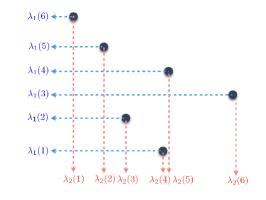
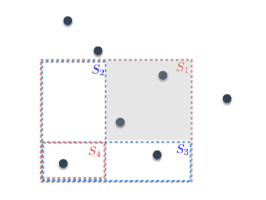
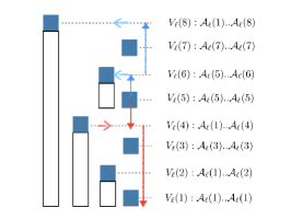
Figure 2: The left figure demonstrates how discretization is carried out when $d=2$, where each of the two dimensions is treated separately and $\lambda_{j}(1)$ through $\lambda_{j}(6)$ record the values on a particular dimension $j\in\{1,2\}$. The middle figure illustrates the inclusion-exclusion principle used to calculate cumulative statistics in the shaded region of interest, by considering $S_{1}-S_{2}-S_{3}+S_{4}$. The right figure depicts the one-dimensional binary indexed tree structure for a toy example of $n=8$ data points, with each $V_{\ell}(\cdot)$ indicating over what region is the cumulative statistics supposed to be calculated. The red arrows indicate the interrogation path when $\mathcal{A}_{\ell}(5)$ is evaluated ($5\to 4\to 0$), and the blue arrows indicate the update path when $T_{\ell}(5)$ is added ($5\to 6\to 8$).

Similar to the definition of $\mathcal{A}_{\ell}(i)$ in the $d=1$ setting, for the general multivariate case define

$$\mathcal{A}_{\ell}(i_{1},\cdots,i_{d})=\sum_{t=1}^{n}\mathbb{I}[\chi_{t1}\leq i_{1},\cdots,\chi_{td}\leq i_{d}]T_{\ell}(X_{t},Y_{t})$$

for $i_{1},\cdots,i_{d}\in[n]$. Suppose for now that $\mathcal{A}_{\ell}(i_{1},\cdots,i_{d})$ are available for all $\ell$ and $i_{1},\cdots,i_{d}$ by some pre-processing procedure. To compute the estimate $\widehat{m}_{n}(z)$, first find $L_{1},\cdots,L_{d}$ and $U_{1},\cdots,U_{d}$ by binary searches, where (for $j=1,\cdots,d$)

$$L_{j} =\arg\max\left\{i:\lambda_{j}(i)<z_{j}-h/2\right\};$$

$$U_{j} =\arg\max\left\{i:\lambda_{j}(i)\leq z_{j}+h/2\right\}.$$ (9)

The sufficient statistics $\mathcal{T}_{\ell}^{z,h}$ can then be computed as

$$\mathcal{T}_{\ell}^{z,h}=\sum_{\nu_{1},\cdots,\nu_{d}\in\{0,1\}^{d}}(-1)^{\nu_{1}+\cdots+\nu_{d}}\mathcal{A}_{\ell}(i_{1}^{(\nu_{1})},\cdots,i_{d}^{(\nu_{d})}),$$

where $i_{j}^{(0)}=U_{j}$ and $i_{j}^{(1)}=L_{j}$. The validity of the computational formula for $\mathcal{T}_{\ell}^{z,h}$ is implied by the inclusion-exclusion principle, and involves $2^{d}$ evaluations of $\mathcal{A}_{\ell}(i_{1},\cdots,i_{d})$. An illustrative example of the $d=2$ case is given in the middle plot of Figure 2.

The question remains to design fast algorithms that compute $\mathcal{A}_{\ell}(i_{1},\cdots,i_{d})$ for arbitrary input tuple $(i_{1},\cdots,i_{d})\in[n]^{d}$. In the basic univariate case of $d=1$, this is accomplished by a sweeping pre-processing that records $\mathcal{A}_{\ell}(i)$ for all $i\in[n]$. Such an approach, however, no longer works for $d>1$ because a sweeping algorithm that records all $\mathcal{A}_{\ell}(i_{1},\cdots,i_{d})$ takes $O(n^{d})$ space and time complexity and is clearly impractical. To overcome this difficulty, we consider a data structure named binary indexed trees and show how it can compute every $\mathcal{A}_{\ell}(i_{1},\cdots,i_{d})$ evaluation in $O(\log^{d}n)$ time.

Input: training set $\{(X_{i},Y_{i})\}_{i=1}^{n}$, testing set $\{z_{i}\}_{i=1}^{s}$, bandwidth $h>0$, dimension $d$, polynomial degree $k$

Output: local polynomial estimates $\{\widehat{m}_{n}(z_{i})\}_{i=1}^{s}$ or $\{\widehat{f}_{n}(z_{i})\}_{i=1}^{s}$

Initialize: hash functions $\hbar_{1},\cdots,\hbar_{d}$ and hash tables $\{\mathcal{H}_{\ell}\}_{\ell=1}^{M}$;

$\triangleright$ pre-processing steps

Discretization: for every $j\in[d]$ sort $\{X_{ij}\}_{i=1}^{n}$ in ascending order and label them $\lambda_{j}(1),\cdots,\lambda_{j}(d)$;

for each $\ell=1,\cdots,M$ and $t=1,\cdots,n$ do

       Compute sufficient statistics $T_{\ell}(X_{t},Y_{t}$) and find $i_{1},\cdots,i_{d}\in[n]$ such that $\lambda_{1}(i_{1})=X_{t1},\cdots,\lambda_{d}(i_{d})=X_{td}$;

       Compute update paths $\textsf{PATH}^{U}(i_{1}),\cdots,\textsf{PATH}^{U}(i_{d})$ using Eq. (11);

       for $i_{1}^{\prime}\in\textsf{PATH}^{U}(i_{1}),i_{2}^{\prime}\in\textsf{PATH}^{U}(i_{2}),\cdots,i_{d}^{\prime}\in\textsf{PATH}^{U}(i_{d})$ do

             Update: $\mathcal{H}_{\ell}(H(i_{1}^{\prime},\cdots,i_{d}^{\prime}))\leftarrow\mathcal{H}_{\ell}(H(i_{1}^{\prime},\cdots,i_{d}^{\prime}))+T_{\ell}(X_{t},Y_{t})$;

       end for

      

end for

$\triangleright$ compute estimates

for each $t=1,\cdots,s$ do

       Find $L_{1},\cdots,L_{d}$ and $U_{1},\cdots,U_{d}$ defined in Eq. (9) for $z_{t}$ and $h$ using binary searches;

       for each $\ell=1,\cdots,M$ do

             for $\nu_{1},\nu_{2},\cdots,\nu_{d}\in\{0,1\}$ do

                   Initialize $\mathcal{A}_{\ell}(i_{1}^{(\nu_{1})},\cdots,i_{d}^{(\nu_{d})})=0$, where $i_{j}^{(0)}=U_{j}$ and $i_{j}^{(1)}=L_{j}$ for $j\in[d]$;

                   Compute interrogation paths $\textsf{PATH}^{I}(i_{1}^{(\nu_{1})}),\cdots,\textsf{PATH}^{I}(i_{d}^{(\nu_{d})})$ using Eq. (10);

                   for $i_{1}^{\prime}\in\textsf{PATH}^{I}(i_{1}^{(\nu_{1})}),\cdots,i_{d}^{\prime}\in\textsf{PATH}^{I}(i_{d}^{\nu_{d}})$ do

                         Accumulate: $\mathcal{A}_{\ell}(i_{1}^{(\nu_{1})},\cdots,i_{d}^{(\nu_{d})})\leftarrow\mathcal{A}_{\ell}(i_{1}^{(\nu_{1})},\cdots,i_{d}^{(\nu_{d})})+\mathcal{H}_{\ell}(H(i_{1}^{\prime},\cdots,i_{d}^{\prime}))$;

                   end for

                  

             end for

            Compute $\mathcal{T}_{\ell}^{z_{t},h}=\sum_{\nu_{1},\cdots,\nu_{d}}(-1)^{\nu_{1}+\cdots+\nu_{d}}\mathcal{A}_{\ell}(i_{1}^{(\nu_{1})},\cdots,i_{d}^{(\nu_{d})})$, using the inclusion-exclusion principle;

            

       end for

      Obtain estimate $\widehat{m}_{n}(z_{t})$ or $\widehat{f}_{n}(z_{t})$ using Eq. (5) and sufficient statistics $\{\mathcal{T}_{\ell}^{z_{t},h}\}_{\ell=1}^{L}$;

      

end for

Algorithm 1 The main accelerated local polynomial regression algorithm.

3.4 Binary indexed trees

The binary indexed tree or Fenwick’s tree, invented and first documented by Fenwick (1994), is a simple yet powerful data structure that supports fast queries and updates of partial sums, corresponding to $\mathcal{A}_{\ell}(i_{1},\cdots,i_{d})$ defined in this paper.

In the rightmost panel of Figure 2 we give a toy example with $n=8$ data points and $d=1$. The $V_{\ell}(i)$ entries for $i=1,\cdots,n$ are the main data structure kept by the binary indexed tree, each corresponding to the cumulative statistics of data points in a specific interval. To query or interrogate a particular partial sum $\mathcal{A}_{\ell}(i)$, one starts with $i$ and repeatedly rips off the least significant bit (LSB) in the binary expansion of $i$ and accumulates the entries of $V_{\ell}$ on the path. For example, for $i=5$ the query/interrogation path would be $5\to 4\to 0$. Formally, the following update rule is applied when interrogating partial sum $\mathcal{A}_{\ell}(i)$:

$$\text{\bf Interrogation}:\;\;i\leftarrow i-\textsc{LSB}(i).$$ (10)

Here $\textsc{LSB}(i)$ denotes the least significant bit of $i$ in its binary expansion.

To add (update) a data point $T_{\ell}(i)$ to the binary indexed tree, one has to undo the interrogation path in Eq. (10). It is easy to verify that the following update procedure is an exact mirroring of the interrogation rule in Eq. (10):

$$\text{\bf Update}:\;\;i\leftarrow i+\textsc{LSB}(i+1).$$ (11)

For example, starting with $i=5$ the updating procedure would take us to $5\to 6\to 8$, meaning that $V_{\ell}(5)$, $V_{\ell}(6)$ and $V_{\ell}(8)$ are updated with the data entry $T_{\ell}(5)$ added.

To simplify notations, we write $\textsf{PATH}^{I}(i)$ and $\textsf{PATH}^{U}(i)$ as the interrogation and update paths starting from $i$, respectively. For example, $\textsf{PATH}^{I}(5)=\{5,4\}$ and $\textsf{PATH}^{U}(5)=\{5,6,8\}$ if $n=8$. It is a simple observation that for any $i\in[n]$, $|\textsf{PATH}^{I}(i)|,|\textsf{PATH}^{U}(i)|=O(\log n)$. Thus, both interrogation and updating operations (for $d=1$) can be completed in $O(\log n)$ time.

To extend the univariate binary indexed tree to higher dimensions, consider tuple $i_{1},\cdots,i_{d}\in[n]^{d}$ at which interrogation or update is needed. For evaluation of $\mathcal{A}_{\ell}(i_{1},\cdots,i_{d})$, accumulate all $V_{\ell}(i_{1}^{\prime},\cdots,i_{d}^{\prime})$ such that $i_{1}^{\prime}\in\textsf{PATH}^{I}(i_{1}),i_{2}^{\prime}\in\textsf{PATH}^{I}(i_{2}),\cdots,i_{d}^{\prime}\in\textsf{PATH}^{I}(i_{d})$ and add them together. Similarly, when adding a data point $T_{\ell}(i_{1},\cdots,i_{d})$, consider all $i_{1}^{\prime}\in\textsf{PATH}^{U}(i_{1}),i_{2}^{\prime}\in\textsf{PATH}^{U}(i_{2}),\cdots,i_{d}^{\prime}\in\textsf{PATH}^{U}(i_{d})$ and update each $V_{\ell}(i_{1}^{\prime},\cdots,i_{d}^{\prime})$ with $T_{\ell}(i_{1},\cdots,i_{d})$. The time complexity for both interrogation and updating is $O(\log^{d}n)$.

3.5 Lazy memory allocation via Hashing

Although the time complexity of $d$-dimensional binary indexed trees is $O(\log^{d}n)$ and is small, the space complexity is another story. A naive implementation of the multi-dimensional binary indexed tree would require $O(n^{d})$ memory to store all $V_{\ell}(i_{1},\cdots,i_{d})$ values. It is imperative to design more intelligent space allocation algorithms that significantly reduce the $O(n^{d})$ space complexity for practical usages.

An important observation of the multi-dimensional binary indexed tree is that the $V_{\ell}$ values are extremely sparse, with most of the entries equal to zero. More specifically, with $n$ points in the training data set, the number of non-zero entries of $V_{\ell}$ is at most $O(n\log^{d}n)$ because each data point is associated with a update path of length at most $O(\log^{d}n)$, which is significantly smaller than $O(n^{d})$. This motivates us to consider a lazy memory allocation scheme based on Hash tables, which would subsequently reduce the space complexity from $O(n^{d})$ to nearly $O(n\log^{d}n)$.

In particular, we construct $M$ hash tables $\{\mathcal{H}_{\ell}\}_{\ell=1}^{M}$ each corresponding to a sufficient statistics $\mathcal{T}_{\ell}$ to be maintained. When adding a new data point $T_{\ell}(i_{1},\cdots,i_{d})$, we insert all entries $i_{1}^{\prime}\in\textsf{PATH}^{U}(i_{1}),\cdots,i_{d}^{\prime}\in\textsf{PATH}^{U}(i_{d})$ into the corresponding Hash table $\mathcal{H}_{\ell}$; similarly when interrogating a point $(i_{1},\cdots,i_{d})$ we read values off all relevant entries $i_{1}^{\prime}\in\textsf{PATH}^{I}(i_{1}),\cdots,i_{d}^{\prime}\in\textsf{PATH}^{I}(i_{d})$ from the Hash table $\mathcal{H}_{\ell}$ and add them together.

Let $b\in\mathbb{N}$ be a pre-determined capacity parameter of hash tables $\{\mathcal{H}_{\ell}\}_{\ell=1}^{M}$ to be constructed, which satisfies $b=\Omega(n\log^{d}n)$. Let $\tau\in\mathbb{N}$ be another pre-defined integer. Suppose $\hbar_{1},\cdots,\hbar_{d}:[n]\to[b]$ are $\tau d$-wise independent hash functions, meaning that for all $j=1,\cdots,d$ and any $i_{1},i_{2},\cdots,i_{\tau d}\in[n]$, $a_{1},\cdots,a_{\tau d}\in[b]$,

$$\Pr\left[\hbar_{j}(i_{1})=a_{1}\wedge\cdots\wedge\hbar_{j}(i_{\tau d})=a_{\tau d}\right]=b^{-\tau d}.$$

A “composite” hash function $H:[n]^{d}\to[b]$ can then be defined as

$$H(i_{1},\cdots,i_{d}):=\left(\hbar_{1}(i_{1})+\cdots+\hbar_{d}(i_{d})\right)\mod b.$$

It is a well-known result that $H$ is a $\tau$-wise independent hash function on $[n]^{d}$ (see for example (Pham and Pagh 2013, Wang et al. 2015)). The corresponding entry of $(i_{1},\cdots,i_{d})\in[n]^{d}$ in the Hash table $\mathcal{H}_{\ell}$ can then be located at

$$\mathcal{H}_{\ell}(H(i_{1},\cdots,i_{d})).$$

When collision occurs, standard methods such as hash chains or linear probing can be employed to resolve collision. In particular, when $\tau=5$ for linear probing, the expected number of collision would be at a constant level (Pagh et al. 2009, Thorup and Zhang 2012).

3.6 Summary of time and space complexity

The capacity of the Hash table constructed in the previous section, $b$, can be set as $b\asymp n\log^{d}n$, leading to the expected number of collision to be upper bounded at a constant level. Hence, the space complexity of the proposed algorithm is $O(n\log^{d}n)$.

For the time complexity, note that each insertion of a data point $x_{i},i\in[n]$ requires $M$ update steps along the update paths in Eq. (11), and each estimate requires $2^{d}M$ interrogation steps along the interrogation paths in Eq. (10). Because $M\leq(2k)^{d}+k^{d}$ and the length of each update/interrogation path is upper bounded by $O(\log^{d}n)$, the total time complexity of Algorithm 1 is upper bounded by $O((2k)^{d}(n+s)\log^{d}n)=O((n+s)\log^{d}n)$, where both $k$ and $d$ are treated as constants.

4 Numerical results

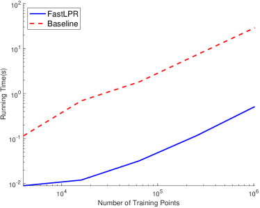
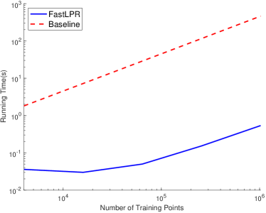
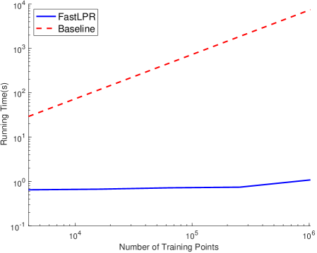
Figure 3: Running times (secs) of fast and baseline implementation of local mean averaging ($k=0$) for univariate data ($d=1$), with varying number of testing points $s=4000$ (left), $s=64000$ (middle) and $s=1024000$ (right).

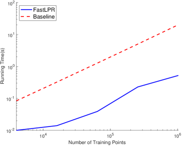
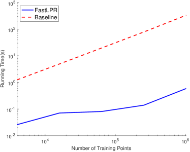
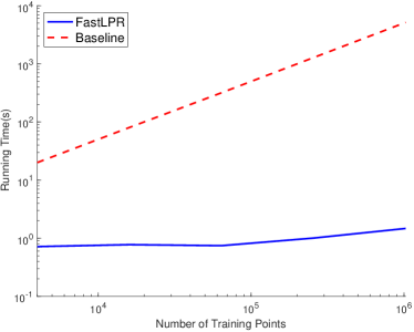
Figure 4: Running times (secs) of fast and baseline implementation of local linear regression ($k=1$) for univariate data ($d=1$), with varying number of testing points $s=4000$ (left), $s=64000$ (middle) and $s=1024000$ (right).

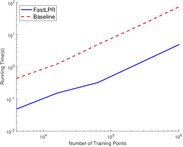
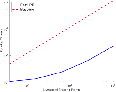
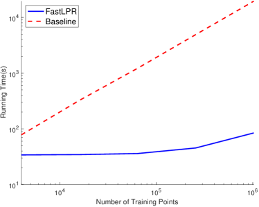
Figure 5: Running times (secs) of fast and baseline implementation of local mean averaging ($k=0$) for bivariate data ($d=2$), with varying number of testing points $s=4000$ (left), $s=64000$ (middle) and $s=1024000$ (right).

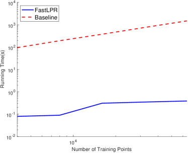
Figure 6: Running times (secs) of fast and baseline implementation of local mean averaging ($k=0$) for bivariate data ($d=3$), with varying number of testing points $s=4000$ (left), $s=16000$ (middle) and $s=64000$ (right).

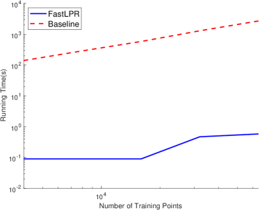
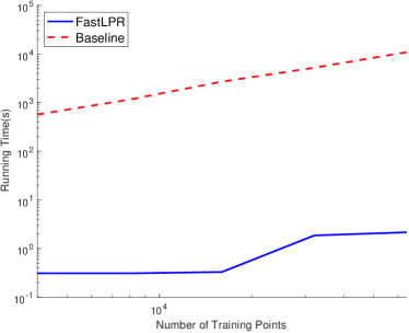
Figure 7: Running times (secs) of fast and baseline implementation of local mean averaging ($k=1$) for bivariate data ($d=3$), with varying number of testing points $s=4000$ (left), $s=16000$ (middle) and $s=64000$ (right).

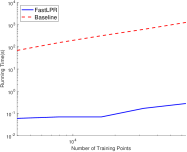
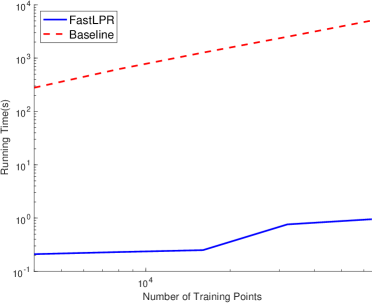
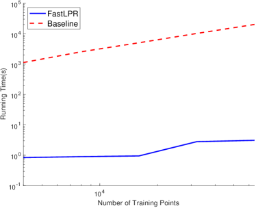
Figure 8: Running times (secs) of fast and baseline implementation of local mean averaging ($k=2$) for bivariate data ($d=3$), with varying number of testing points $s=4000$ (left), $s=16000$ (middle) and $s=64000$ (right).

In this section we use simulations to verify the effectiveness of our proposed algorithm. All source codes of our implementation are provided in the supplementary materials accompanying this paper. The raw data and results in the plotted figures and tables are also provided in a separate online supplement.

We implement algorithm 1 using C++. All simulations are done on a computer installed with uBuntu 14.04 LTS 64bit OS, 31.4 Gib Memory, Intel Core i7-4970 CPU @3.60GHz x 8, except for the running time reported for our own implementation of the brute-force algorithm which is experimented on a MacBook Pro laptop with macOS Mojave 10.14.6, 16GB memory, 2.3 GHz Intel Core i9 because the former server has been de-serviced at the time this part of the experiment is carried out.

Two baselines are considered and compared against our proposed method. The first baseline is a widely used R library locpol, which is implemented in C. A detailed description of the locpol package can be found in (Cabrera 2012). The relevant routines in locpol include locCteSmootherC, locLinSmootherC, locCuadSmootherC and locPolSmootherC, corresponding to local polynomial estimation of $k=0$, $k=1$, $k=2$ and $k>2$, respectively. Note that for $d\geq 2$ only local constant regression (i.e., $k=0$) is supported in locpol. While the detailed implementation strategy of locpol is not available, judging from the high computational costs in numerical experiments we conjecture that the naive brute-force implementation is used which computes $\widehat{\theta}_{n}$ separately for each data point.

The second baseline is our own implementation of the brute-force computation of local polynomial estimates, which serves as a second baseline for comparison. We implement the brute-force approach using C++, which supports general data dimension $d$ and polynomial degree $k$.

	Our implementation (MB)	Baseline (MB)
$k=0,n=4000$	72	1.3
$k=0,n=8000$	170	1.4
$k=0,n=16000$	432	2.3
$k=0,n=32000$	1044	3.7
$k=0,n=64000$	2485	6.3
$k=1,n=4000$	73	1.3
$k=1,n=8000$	181	1.6
$k=1,n=16000$	443	2.5
$k=1,n=32000$	2221	3.9
$k=1,n=64000$	4945	6.6
$k=2,n=4000$	354	4.2
$k=2,n=8000$	897	8.5
$k=2,n=16000$	2217	16.5
$k=2,n=32000$	5280	28.4
$k=2,n=64000$	7642	52.8

Table 1: Comparison of memory consumption between our method and the naive method. For all experiments we fix $d=3$ and $s=4000$.

We first compare the running times of our fast local polynomial regression implementation (Algorithm 1, denoted as FastLPR) with the baseline R package locpol under various simulation settings in Figure 3 ($d=1,k=0$), Figure 4 ($d=1,k=1$) and Figure 5 ($d=2,k=0$). The ground-truth functions $f:\mathbb{R}^{d}\to\mathbb{R}$ are defined as $f(x_{1},\cdots,x_{d})=\sum_{i=1}^{d}\sin(x_{i})$. Note that for $d=2$ we only experiment with local mean averaging ($k=0$) because the locpol package only supports $k=0$ for $d>1$. For all experimental setups, the running times are reported under varying number of training and testing points, all uniformly sampled from the unit cube $[0,1]^{d}$.

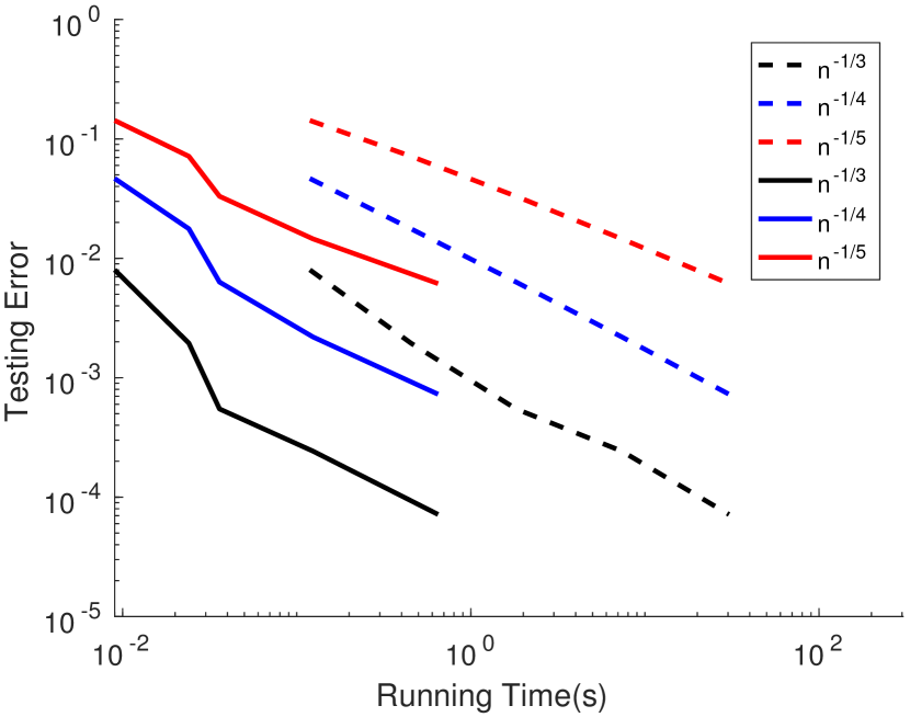
(a) local constant regression ($k=0$)

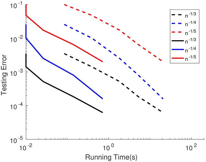
(b) local linear regression ($k=1$)

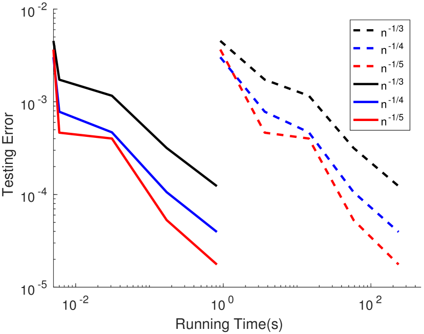
(c) local quadratic regression ($k=2$)

Figure 9: Local polynomial regression for one dimensional data with running time constraints. Solid lines correspond to FastLPR and dot lines correspond to BaseLine.

From Figures 3, 4 and 5, we observe that as the number of testing points ($s$) or the training points become larger, the advantages of our proposed algorithm are more significant. In particular, when 1,024,000 training and testing points are present under the setting of $k=1$ and $d=1$, Algorithm 1 achieves $40,000\times$ speed-up over the naive implementation in locpol. The reason is that the naive implementation has $\Theta\left(ns\right)$ time complexity whereas ours is $O\left((n+s)\log^{d}n\right)$.

We compare our algorithm with a baseline implementation of local polynomial regression in Figures 6, 7, 8 on 3-dimensional data (i.e., $d=3$) with polynomial degrees ranging from $k=0$ to $k=2$. Because the locpol package in R only supports $k=0$ for $d>1$, we compare our proposed algorithm with our own brute-force implementation of local polynomial regression in C++. As we can observe from the figures, our proposed algorithm still consistently outperforms the baseline implementation for all polynomial degrees in the case of $d=3$.

We also compare memory consumptions between our method and the naive method in Table 1. For all experiments we fix $d=3$ and $s=4000$ (we found different $s$ do not affect the memory consumption of both methods by much). As we can observe from Table 1, our implementation consumes significantly more memory compared to baseline because the multi-dimensional binary indexed trees is quite a memory-intensive data structure, even with lazy memory allocation schemes in place. Nevertheless, the highest amount of memory consumption (approximately 7GB for $d=3$, $k=2$ and $n=64,000$) is still well within the limit of modern main memories on desktop or workspace computers. Such memory consumption is worthy because of the significant improvement in running time our proposed algorithm brings.

Lastly, we report in Figure 9 the function reconstruction errors of both FastLPR and the baseline method in locpol under fixed running time budgets. We fix number of testing points to be $4000$ and the bandwidth parameter $h$ takes values of $n^{-1/3}$, $n^{-1/4}$ and $n^{-1/5}$. Figure 9 shows under given time budgets, our proposed FastLPR algorithm processes much more observations (training samples) and therefore achieves significantly smaller reconstruction error.

5 Discussion

Kernel functions.

In our accelerated local polynomial estimation algorithm, the kernel $K(\cdot)$ is assumed to be the box kernel $K(u)=\mathbb{I}[|u|\leq 1/2]$ and for multiple dimensions ($d\geq 2$) the “composite kernel” is defined in terms of $\ell_{\infty}$ norm, meaning that the kernel evaluation between $x,z\in\mathbb{R}^{d}$ is $K(\|x-z\|_{\infty}/h)$. The box kernel ensures that the sufficient statistics can be expressed as a linear combination of unweighted partial sums, and the $\ell_{\infty}$ norm in multi-variate kernel evaluations lead to rectangle regions whose edges are parallel to the standard basis. Both properties are crucial for our algorithmic development that enables fast sufficient statistics computation via binary indexed trees.

In general, box kernels with $\ell_{\infty}$ distance measures are sufficient as they achieve the same minimax statistical efficiency as other kernel functions and/or equivalent distance measures. However, for certain applications it might be desirable to consider kernel functions smoother than the box kernel (e.g., the Gaussian kernel $K(u)=e^{-u^{2}/2}/\sqrt{2\pi}$) to obtain smoother function fits. We believe significantly different techniques are required to handle such kernels that are non-uniform and not restricted to parallel rectangular neighborhoods of testing points.

Incremental training and testing sets.

While in the description of our algorithm the sizes of both training and testing sets ($n$ and $s$) are fixed a priori, we remark that our algorithm can perfectly handle training and testing data with increasing sizes. In particular, for every new training or testing point, the corresponding update or interrogation paths are calculated in $O(\log^{d}n)$ time and the Hash tables can be updated/queried using a similar amount of running time. This property is particularly useful in applications where training data constantly grow/change, and estimates on incoming test points have to be made in a real-time fashion.

Further acceleration with approximate computation.

In cases where exact computations of local polynomial estimates are not mandatory and small error in the estimates can be tolerated, it is possible to further reduce the time and space complexity beyond $O(n\log^{d}n)$.

One approach is to consider significantly smaller (shorter) Hash tables with capacity $b\ll n\log^{d}n$. Because the capacity of Hash tables is significantly smaller than the number of entries created by binary indexed trees, collisions are unavoidable. Instead of resolving collisions completely, one can borrow the ideas of CountSketch (Charikar et al. 2004) that multiplies an additional Rademacher variable $\sigma(i_{1},\cdots,i_{d})$ in Hash table updates:

$$\mathcal{H}_{\ell}(H(i_{1},\cdots,i_{d})) \leftarrow\mathcal{H}_{\ell}(H(i_{1},\cdots,i_{d}))$$

$$\;\;\;\;+\sigma(i_{1},\cdots,i_{d})T_{\ell}(i_{1},\cdots,i_{d}).$$

Dependency on data dimension $d$.

The time complexity of our proposed algorithm has a leading $O((2k)^{d})$ term which scales exponentially with data dimension $d$, which is dropped in the main $O((n+s)\log^{d}n)$ time complexity bound because both polynomial degree $k$ and data dimension $d$ are treated as constants in this paper. On the other hand, the naive approach has an $O(n^{2})$ time complexity and does not explicitly depend exponentially on $d$. Nevertheless, in nonparametric regression/estimation it is typical that an exponential number of sample points are required (e.g., to estimate a Lipschitz continuous function up to precision $\varepsilon$, $\Omega(\varepsilon^{-(2+d)})$ samples are needed (Tsybakov 2009)). Hence, our $O((n+s)\log^{d}n)$ time complexity is generally much more preferable than the $O(n^{2})$ time complexity of naive approaches.

6 Conclusion

In this paper we propose nearly linear time algorithms that compute local polynomial estimates for nonparametric density and regression function estimates. Our algorithm is based on the novel application of multivariate binary indexed trees together with discretization and hashing techniques. Simulation results demonstrate an up to $40000\times$ speed-up over state-of-the-art R implementation of local polynomial regression. Future directions including general kernel functions and further algorithmic acceleration via sketching approximation are discussed.

References

- Cabrera (2012) Cabrera JLO (2012) locpol: Kernel local polynomial regression. URL http://mirrors.ustc.edu.cn/CRAN/web/packages/locpol/index.html .
- Cai (1999) Cai TT (1999) Adaptive wavelet estimation: a block thresholding and oracle inequality approach. The Annals of Statistics 27(3):898–924.
- Cattaneo et al. (2017) Cattaneo MD, Jansson M, Ma X (2017) Simple local polynomial density estimators. Technical report, Working Paper. Retrieved July 22, 2017 from http://wwwpersonal. umich. edu/~ cattaneo/papers/Cattaneo-Jansson-Ma_2017_LocPolDensity. pdf.
- Charikar et al. (2004) Charikar M, Chen K, Farach-Colton M (2004) Finding frequent items in data streams. Theoretical Computer Science 312(1):3–15.
- Cheng et al. (1997) Cheng MY, Fan J, Marron JS (1997) On automatic boundary corrections. The Annals of Statistics 25(4):1691–1708.
- Choi et al. (2018) Choi TM, Wallace SW, Wang Y (2018) Big data analytics in operations management. Production and Operations Management 27(10):1868–1883.
- De Boor (1978) De Boor C (1978) A practical guide to splines, volume 27 (Springer-Verlag New York).
- Donoho et al. (1998) Donoho DL, Johnstone IM, et al. (1998) Minimax estimation via wavelet shrinkage. The Annals of Statistics 26(3):879–921.
- Donoho and Johnstone (1994) Donoho DL, Johnstone JM (1994) Ideal spatial adaptation by wavelet shrinkage. Biometrika 81(3):425–455.
- Fan (1993) Fan J (1993) Local linear regression smoothers and their minimax efficiencies. The Annals of Statistics 21(1):196–216.
- Fan and Gijbels (1992) Fan J, Gijbels I (1992) Variable bandwidth and local linear regression smoothers. The Annals of Statistics 20(4):2008–2036.
- Fan and Gijbels (1996) Fan J, Gijbels I (1996) Local polynomial modelling and its applications (CRC Press).
- Fenwick (1994) Fenwick PM (1994) A new data structure for cumulative frequency tables. Software: Practice and Experience 24(3):327–336.
- Friedman et al. (2001) Friedman J, Hastie T, Tibshirani R (2001) The elements of statistical learning, volume 1 (Springer series in statistics New York).
- Geer (2000) Geer SA (2000) Empirical Processes in M-estimation, volume 6 (Cambridge university press).
- Green and Silverman (1993) Green PJ, Silverman BW (1993) Nonparametric regression and generalized linear models: a roughness penalty approach (CRC Press).
- Györfi et al. (2006) Györfi L, Kohler M, Krzyzak A, Walk H (2006) A distribution-free theory of nonparametric regression (Springer Science & Business Media).
- Härdle et al. (2012) Härdle W, Kerkyacharian G, Picard D, Tsybakov A (2012) Wavelets, approximation, and statistical applications, volume 129 (Springer Science & Business Media).
- Hastie and Loader (1993) Hastie T, Loader C (1993) Local regression: Automatic kernel carpentry. Statistical Science 8(2):120–129.
- Hazen et al. (2018) Hazen BT, Skipper JB, Boone CA, Hill RR (2018) Back in business: Operations research in support of big data analytics for operations and supply chain management. Annals of Operations Research 270(1-2):201–211.
- Larry (2006) Larry W (2006) All of nonparametric statistics (Springer Texts in Statistics. New York: Springer Science+ Business Media).
- Lepski et al. (1997) Lepski OV, Mammen E, Spokoiny VG (1997) Optimal spatial adpaptation to inhomogeneous smoothness: an approach based on kernel estimates with variable bandwidth selectors. The Annals of Statistics 25(3):929–947.
- Mišić and Perakis (2019) Mišić V, Perakis G (2019) Data analytics in operations management: A review. Manufacturing & Services Operations Management 22(1):158–169.
- Pagh et al. (2009) Pagh A, Pagh R, Ruzic M (2009) Linear probing with constant independence. SIAM Journal on Computing 39(3):1107–1120.
- Pham and Pagh (2013) Pham N, Pagh R (2013) Fast and scalable polynomial kernels via explicit feature maps. Proceedings of the ACM SIGKDD international conference on Knowledge discovery and data mining (KDD).
- Reinsch (1967) Reinsch CH (1967) Smoothing by spline functions. Numerische Mathematik 10(3):177–183.
- Thorup and Zhang (2012) Thorup M, Zhang Y (2012) Tabulation-based 5-independent hashing with applications to linear probing and second moment estimation. SIAM Journal on Computing 41(2):293–331.
- Tsybakov (2009) Tsybakov AB (2009) Introduction to nonparametric estimation. (Springer Series in Statistics. Springer, New York).
- Wang et al. (2015) Wang Y, Tung HY, Smola AJ, Anandkumar A (2015) Fast and guaranteed tensor decomposition via sketching. Proceedings of Advances in Neural Information Processing Systems (NIPS).
- Wang et al. (2014) Wang YX, Smola A, Tibshirani R (2014) The falling factorial basis and its statistical applications. Proceedings of the International Conference on Machine Learning (ICML).
- Whittaker (1922) Whittaker ET (1922) On a new method of graduation. Proceedings of the Edinburgh Mathematical Society 41:63–75.