A representer theorem for deep neural networks

Abstract

We propose to optimize the activation functions of a deep neural network by adding a corresponding functional regularization to the cost function. We justify the use of a second-order total-variation criterion. This allows us to derive a general representer theorem for deep neural networks that makes a direct connection with splines and sparsity. Specifically, we show that the optimal network configuration can be achieved with activation functions that are nonuniform linear splines with adaptive knots. The bottom line is that the action of each neuron is encoded by a spline whose parameters (including the number of knots) are optimized during the training procedure. The scheme results in a computational structure that is compatible with existing deep-ReLU, parametric ReLU, APL (adaptive piecewise-linear) and MaxOut architectures. It also suggests novel optimization challenges, while making the link with $\ell_{1}$ minimization and sparsity-promoting techniques explicit.

Keywords: splines, regularization, sparsity, learning, deep neural networks, activation functions

1 Introduction

The basic regression problem in machine learning is to find a parametric representation of a function $f:\mathbb{R}^{N}\to\mathbb{R}$ given a set of data points $({\boldsymbol{x}}_{m},y_{m})\in\mathbb{R}^{N+1}$ such that $f({\boldsymbol{x}}_{m})$ is close to $y_{m}$ for $m=1,\dots,M$ in an appropriate sense (Bishop, 2006). Classically, there are two steps involved. The first is the design, which can be abstracted in the choice of a given parametric class of functions ${\boldsymbol{x}}\mapsto f({\boldsymbol{x}}|{\boldsymbol{\theta}})$, where ${\boldsymbol{\theta}}$ encodes the parameters. For instance, $f({\boldsymbol{x}}|{\boldsymbol{\theta}})$ could be a neural network with weights ${\boldsymbol{\theta}}$. The second is the training, which basically amounts to an interpolation/approximation problem where the chosen model is fit to the data. In practice, the optimal parameter ${\boldsymbol{\theta}}_{0}$ is determined via the functional minimization

$${\boldsymbol{\theta}}_{0}=\arg\min_{{\boldsymbol{\theta}}}\sum_{m=1}^{M}E\big{(}y_{m},f({\boldsymbol{x}}_{m}|{\boldsymbol{\theta}})\big{)},$$ (1)

where $E:\mathbb{R}\times\mathbb{R}\to\mathbb{R}^{+}$ is a convex error function that quantifies the discrepancy of the fit to the data. A classical choice is $E\big{(}y_{m},f({\boldsymbol{x}}_{m}|{\boldsymbol{\theta}})\big{)}=|y_{m}-f({\boldsymbol{x}}_{m}|{\boldsymbol{\theta}})|^{2}$, which yields the least-squares solution.

The most delicate step is the design, because it has to deal with two conflicting requirements. First is the desire for universality, meaning that the parametric model $f({\boldsymbol{x}}|{\boldsymbol{\theta}})$ should be flexible enough to allow for the faithful representation of a large class of functions—ideally, the complete family of continuous functions $\mathbb{R}^{N}\to\mathbb{R}$, as the dimensionality of ${\boldsymbol{\theta}}$ goes to infinity. Second is the quest for parsimony, meaning that the model should have a small number of parameters, which leads to an increase in robustness and trustworthiness.

This work aims at unifying the design of neural networks based on variational principles inspired by kernel methods. To set up the stage, we now briefly review the two relevant approaches to supervised learning.

1.1 Kernel methods

A kernel estimator is a linear model with adjustable parameters ${\boldsymbol{\theta}}=(a_{1},\dots,a_{M})\in\mathbb{R}^{M}$ and predefined data centers ${\boldsymbol{x}}_{1},\dots,{\boldsymbol{x}}_{M}\in\mathbb{R}^{N}$ of the form

$$f({\boldsymbol{x}}|{\boldsymbol{\theta}})=\sum_{m=1}^{M}a_{m}h({\boldsymbol{x}},{\boldsymbol{x}}_{m}),$$ (2)

where ${\boldsymbol{x}}\in\mathbb{R}^{N}$ is the input variable of the model and where $h:\mathbb{R}^{N}\times\mathbb{R}^{N}\to\mathbb{R}$ is a positive-definite kernel, a preferred choice being the Gaussian kernel $h({\boldsymbol{x}},{\boldsymbol{y}})=\mathrm{e}^{-\tfrac{1}{2}\|{\boldsymbol{x}}-{\boldsymbol{y}}\|^{2}/\sigma^{2}}$ (Hofmann et al., 2008; Alvarez et al., 2012). This expansion is at the heart of the whole class of kernels methods, including radial-basis functions and support-vector machines (Schölkopf et al., 1997; Vapnik, 2013; Schölkopf and Smola, 2002).

The elegance of kernel estimators lies in that they can be justified based on regularization theory (Poggio and Girosi, 1990; Evgeniou et al., 2000; Poggio and Smale, 2003). The incentive there is to remove some of the arbitrariness of model selection by formulating the learning task as a global minimization problem that takes care of the design and training jointly. The property that makes such an integrated approach feasible is that any Hilbert space ${\mathcal{H}}$ of continuous functions on $\mathbb{R}^{N}$ has a unique reproducing kernel $h_{\mathcal{H}}:\mathbb{R}^{N}\times\mathbb{R}^{N}\to\mathbb{R}$ such that (i) $h_{\mathcal{H}}(\cdot,{\boldsymbol{x}}_{m})\in{\mathcal{H}}$; and (ii) $\langle f,h_{\mathcal{H}}(\cdot,{\boldsymbol{x}}_{m})\rangle_{{\mathcal{H}}}=f({\boldsymbol{x}}_{m})$ for any ${\boldsymbol{x}}_{m}\in\mathbb{R}^{N}$ and $f\in{\mathcal{H}}$ (Aronszajn, 1950). The idea, then, is to formulate the “regularized” version of Problem (1) as

$$f_{\rm RKHS}=\arg\min_{f\in{\mathcal{H}}}\left(\sum_{m=1}^{M}E\big{(}y_{m},f({\boldsymbol{x}}_{m})\big{)}+\lambda\|f\|^{2}_{{\mathcal{H}}}\right),$$ (3)

where the second term penalizes solutions with a large $\|\cdot\|_{\mathcal{H}}$-norm and $\lambda\in\mathbb{R}^{+}$ is an adjustable tradeoff factor. Under the assumption that the loss function $E$ is convex, the representer theorem (Kimeldorf and Wahba, 1971; Schölkopf et al., 2001; Schölkopf and Smola, 2002) then states that the solution of (3) exists, is unique, and such that $f_{\rm RKHS}\in{\rm span}\{h_{\mathcal{H}}(\cdot,{\boldsymbol{x}}_{m})\}_{m=1}^{M}$. This ultimately results in the same linear expansion as (2). The argument also applies the other way round since any positive-definite kernel $h$ specifies a unique reproducing-kernel Hilbert space (RKHS) ${\mathcal{H}}_{h}$, which then provides the regularization functional $\|f\|_{{\mathcal{H}}_{h}}^{2}$ in (3) that is matched to the kernel estimator specified by (2).

The other remarkable feature of kernel expansions is their universality, under mild conditions on $h$ (Micchelli et al., 2006). In other words, one has the guarantee that the generic linear model of (2) can reproduce any continuous function $f:\mathbb{R}^{N}\to\mathbb{R}$ to a desired degree of accuracy by including sufficiently many centers, with the error vanishing as $M\to\infty$. Moreover, because of the tight connection between kernels, RKHS, and splines (de Boor and Lynch, 1966; Micchelli, 1986; Wahba, 1990), one can invoke standard results in approximation theory to obtain quantitative estimates of the approximation error of smooth functions as a function of $M$ and of the widest gap between data centers (Wendland, 2005). Finally, there is a well-known link between kernel methods derived from regularization theory and neural networks, albeit “shallow” ones that involve a single nonlinear layer (Poggio and Girosi, 1990).

1.2 Deep neural networks

While kernel methods have been a major (and winning) player in machine learning since the mid ’90s, they have been recently outperformed by deep neural networks (DNNs) in many real-world applications such as image classification (Krizhevsky et al., 2012), speech recognition (Hinton et al., 2012), and image segmentation (Ronneberger et al., 2015).

The leading idea of deep learning is to build more powerful learning architectures via the stacking/composition of simpler entities (see the review papers by LeCun, Bengio and Hinton (LeCun et al., 2015) and Schmidhuber (Schmidhuber, 2015) and the recent textbook (Goodfellow et al., 2016) for more detailed explanations). In this work, we focus on the popular class of feedforward networks that involve a layered composition of affine transformations (linear weights) and pointwise nonlinearities. The deep structure of such a network is specified by its node descriptor $(N_{0},N_{1},\dots,N_{L})$ where $L$ is the total number of layers (depth of the network) and $N_{\ell}$ is the number of neurons at the $\ell$th layer. The action of a (scalar) neuron (or node) indexed by $(n,\ell)$ is described by the relation $\sigma({\bf{w}}_{n,\ell}^{T}{\boldsymbol{x}}-b_{n,\ell})$ where ${\boldsymbol{x}}\in\mathbb{R}^{N_{\ell-1}}$ denotes the multivariate input of the neuron, $\sigma:\mathbb{R}\to\mathbb{R}$ is a predefined activation function (such as a sigmoid or a ReLU=rectified linear unit), ${\bf{w}}_{n,\ell}\in\mathbb{R}^{N_{\ell-1}}$ a set of linear weights, and $b_{n,\ell}\in\mathbb{R}$ an additive bias. The outputs of layer $\ell$ are then fed as inputs of layer $(\ell+1)$, and so forth for $\ell=1,\dots,L$.

To obtain a global description, we group the neurons within a given layer $\ell$ and specify the two corresponding vector-valued maps:

1. Linear step ${\boldsymbol{f}}_{\ell}:\mathbb{R}^{N_{\ell-1}}\to\mathbb{R}^{N_{\ell}}$ (affine transformation)

   $${\boldsymbol{f}}_{\ell}:{\boldsymbol{x}}\mapsto{\boldsymbol{f}}_{\ell}({\boldsymbol{x}})={\bf{W}}_{\ell}{\boldsymbol{x}}-{\bf{b}}_{\ell}$$ (4)

   with weighting matrix ${\bf{W}}_{\ell}=[{\bf{w}}_{1,\ell}\cdots{\bf{w}}_{N_{\ell},\ell}]^{T}\in\mathbb{R}^{N_{\ell}\times N_{\ell-1}}$ and bias vector ${\bf{b}}_{\ell}=(b_{1,\ell},\dots,b_{N_{\ell},\ell})\in\mathbb{R}^{N_{\ell}}$.

2. Nonlinear step ${\boldsymbol{\sigma}}_{\ell}:\mathbb{R}^{N_{\ell}}\to\mathbb{R}^{N_{\ell}}$ (activation functions)

   $${\boldsymbol{\sigma}}_{\ell}:{\boldsymbol{x}}=(x_{1},\dots,x_{N_{\ell}})\mapsto{\boldsymbol{\sigma}}_{\ell}({\boldsymbol{x}})=\big{(}\sigma_{1,\ell}(x_{1}),\dots,\sigma_{N_{\ell},\ell}(x_{N_{\ell}})\big{)}$$ (5)

   with the possibility of adapting the scalar activation functions $\sigma_{n,\ell}$ on a per-node basis.

This allows us to describe the overall action of the full $L$-layer deep network by

$${\bf{f}}_{\rm deep}({\boldsymbol{x}})=\left({\boldsymbol{\sigma}}_{L}\circ{\boldsymbol{f}}_{L}\circ{\boldsymbol{\sigma}}_{L-1}\circ\cdots\circ{\boldsymbol{\sigma}}_{2}\circ{\boldsymbol{f}}_{2}\circ{\boldsymbol{\sigma}}_{1}\circ{\boldsymbol{f}}_{1}\right)({\boldsymbol{x}}),$$ (6)

which makes its compositional structure explicit. The design step therefore consists in fixing the architecture of the deep neural net: One must specify $(N_{0},N_{1},\dots,N_{L})$ together with the activation functions ${\boldsymbol{\sigma}}_{\ell}:\mathbb{R}^{N_{\ell}}\to\mathbb{R}^{N_{\ell}}$. The activations are traditionally chosen to be not only the same for all neurons within a layer, but also the same across layers. This results in a computational structure with adjustable parameters ${\boldsymbol{\theta}}=({\bf{W}}_{1},\dots,{\bf{W}}_{L},{\bf{b}}_{1},\dots,{\bf{b}}_{L})$ (weights of the linear steps). These are then set during training via the minimization of (1), which is achieved by stochastic gradient descent with efficient error backpropagation (Rumelhart et al., 1986).

While researchers have considered a variety of possible activation functions, such as the traditional sigmoid, a preferred choice that has emerged over the years is the rectified linear unit: ${\rm ReLU}(x)\stackrel{{\scriptstyle\vartriangle}}{{=}}\max(x,0)$ (Glorot et al., 2011). The reasons that support this choice are multiple. The initial motivation was to promote sparsity (in the sense of decreasing the number of active units), capitalizing on the property that ReLU acts as a gate and works well in combination with $\ell_{1}$-regularization (Glorot et al., 2011). Second is the empirical observation that the training of very deep networks is much faster if the hidden layers are composed of ReLU activation functions (LeCun et al., 2015). Last but not least is the connection between deep ReLU networks and splines—to be further developed in this paper.

A key observation is that a deep ReLU network implements a multivariate input-output relation that is continuous and piecewise-linear (CPWL) (Montufar et al., 2014). This remarkable property is due to the ReLU itself being a linear spline, which has prompted Poggio et al. to interpret deep neural networks as hierarchical splines (Poggio et al., 2015). Moreover, it has been shown that any CPWL function admits a deep ReLU implementation (Wang and Sun, 2005; Arora et al., 2016), which is quite significant since the CPWL family has universal approximation properties.

The ability of splines to effectively represent arbitrary (univariate) functions (de Boor, 1978; Schumaker, 1981; Unser, 1999) has also been exploited at the more local level of a neuron/node in a network. Several authors have proposed to use spline-related parametric models to optimize the shape of neural activation units. Existing designs include B-spline receptive fields (Lane et al., 1991), Catmul-Rom splines (Vecci et al., 1998), cubic spline activations (Guarnieri et al., 1999), adaptive piecewise-linear (APL) units (Agostinelli et al., 2015), and smooth piecewise-polynomial functions (Hou et al., 2017).

1.3 Road map

Our purpose in this paper is to strengthen the connection between splines and multilayer ReLU networks even further. To that end, we formulate the design of a deep neural network globally within the context of regularization theory, in direct analogy with the variational formulation of kernel estimators given by (3). The critical aspect, of course, is the selection of an appropriate regularization functional which, for reasons that will be exposed next, will take us outside of the traditional realm of RKHS.

Having set the deep architecture of the neural network, we then formulate the training as a global optimization task whose outcome is a combined set of optimal neuronal activation functions and linear weights. The foundational role of the representer theorem (Theorem 3) is that it will provide us with the parametric representation of the optimal activations, which can then be leveraged for obtaining a numerical implementation that is compatible with current architectures; in particular, the popular deep RELU networks.

2 From deep neural networks to deep splines

Given the generic structure of a deep neural network, we are interested in investigating the possibility of optimizing the shape of the activation function(s) on a node-by-node basis. We now show how this can be achieved within the context of infinite-dimensional regularization theory.

2.1 Choice of regularization functional

For practical relevance, the scheme should favor simple solutions such as an identity or a linear scaling. This will retain the possibility of performing a classical linear regression. It is also crucial that the activation function $\sigma$ be differentiable to be compatible with the chain rule when the backpropagation algorithm is used to train the network. Lastly, we want to promote activation functions that are locally linear (such as the ReLU) since these appear to work best in practice. If the two aforementioned constraints are satisfied, then the activation function is CPWL. As this property is conserved through (multivariate) composition, it implies that the resulting map ${\boldsymbol{f}}_{\rm deep}:\mathbb{R}^{N_{0}}\to\mathbb{R}^{N_{L}}$ is CPWL as well, which is highly desirable for applications Strang (2018). Hence, an idealized solution would be a function $\sigma:\mathbb{R}\to\mathbb{R}$ whose second derivative vanishes almost everywhere.

As measure of sparsity, we use the “total-variation” norm $\|\cdot\|_{\mathcal{M}}$ associated with the Banach space

$${\mathcal{M}}(\mathbb{R})=\{f\in{\mathcal{S}}^{\prime}(\mathbb{R}):\|f\|_{{\mathcal{M}}}\stackrel{{\scriptstyle\vartriangle}}{{=}}{\sup_{\varphi\in{\mathcal{S}}(\mathbb{R}):\|\varphi\|_{\infty}\leq 1}\langle f,\varphi\rangle}<\infty\}$$ (7)

where ${\mathcal{S}}^{\prime}(\mathbb{R})$ is Schwartz’s space of tempered distributions, which is the continuous dual of ${\mathcal{S}}(\mathbb{R})$ (the space of smooth and rapidly-decreasing test functions on $\mathbb{R}$). Note that our definition of $\|\c{[}ot\|_{\mathcal{M}}$ (by duality) is equivalent to the notion of total-variation used in measure theory (Rudin, 1987). The critical point for us is that the latter is a slight extension of the $L_{1}$-norm: The basic property is that $\|f\|_{L_{1}}\stackrel{{\scriptstyle\vartriangle}}{{=}}\int_{\mathbb{R}}|f(x)|{\rm d}x=\|f\|_{{\mathcal{M}}}$ for any $f\in L_{1}(\mathbb{R})$, which implies that $L_{1}(\mathbb{R})\subseteq{\mathcal{M}}(\mathbb{R})$. However, the shifted Dirac distribution $\delta(\cdot-x_{m})\notin L_{1}(\mathbb{R})$ for any shift $x_{m}\in\mathbb{R}$, while $\delta(\cdot-x_{m})\in{\mathcal{M}}(\mathbb{R})$ with $\|\delta(\cdot-x_{m})\|_{{\mathcal{M}}}=1$, which shows that the space ${\mathcal{M}}(\mathbb{R})$ is (slightly) larger than $L_{1}(\mathbb{R})$.

To favor neuronal activation functions $\sigma:\mathbb{R}\to\mathbb{R}$ with “sparse” second derivatives, we shall therefore impose a bound on their second total-variation, which is defined as

$${\rm TV}^{(2)}(\sigma)\stackrel{{\scriptstyle\vartriangle}}{{=}}\|{\rm D}^{2}\sigma\|_{{\mathcal{M}}}={\sup_{\varphi\in{\mathcal{S}}(\mathbb{R}):\|\varphi\|_{\infty}\leq 1}}\langle{\rm D}^{2}\sigma,\varphi\rangle$$

where ${\mathrm{D}}^{2}=\frac{{\rm d}^{2}}{{\rm d}x^{2}}$ is the second derivative operator. The connection with ReLU is that ${\rm D}^{2}\{{\rm ReLU}\}=\delta$, which confirms that the ReLU activation function is intrinsically sparse with ${\rm TV}^{(2)}({\rm ReLU})=1$.

Since our formulation involves a joint optimization of all network components, it is important to decouple the effect of the various stages. The only operation that is common to linear transformations and pointwise nonlinearities is a linear scaling, which is therefore transferable from one level to the next. Since most regularization schemes are scale-sensitive, it is essential to prevent such a transfer. We achieve this by restricting the class of admissible weight vectors ${\bf{w}}_{n,\ell}$ acting on a given node indexed by $({n,\ell})$ to those that have a unit norm. In other words, we shall normalize the scale of all linear modules with the introduction of the new variable ${\bf{u}}_{n,\ell}={\bf{w}}_{n,\ell}/\|{\bf{w}}_{n,\ell}\|$.

2.2 Supporting optimality results

As preparation for our representer theorem, we present a lemma on the ${\rm TV}^{(2)}$-optimality of piecewise-linear interpolation. This enabling result is deduced from the general spline theory presented in (Unser et al., 2017), as detailed in the appendix. We then provide arguments to disqualify the use of the more conventional Sobolev-type regularization.

The formal definition of our native space (i.e., the space over which the optimization is performed) is

$${\rm BV}^{(2)}(\mathbb{R})=\{f:\mathbb{R}\to\mathbb{R}:\|{\rm D}^{2}f\|_{{\mathcal{M}}}<\infty\},$$ (8)

which is the class of functions with bounded second total variation. As explained in Appendix B, we can endow ${\rm BV}^{(2)}(\mathbb{R})$ with the norm

$$\|f\|_{{\rm BV}^{(2)}}\stackrel{{\scriptstyle\vartriangle}}{{=}}\|{\rm D}^{2}f\|_{{\mathcal{M}}}+\sqrt{|f(0)|^{2}+|f(1)-f(0)|^{2}},$$ (9)

which turns it into a bona fide Banach space. We can then also guarantee that this space is large enough—i.e., ${\mathcal{S}}(\mathbb{R})\subseteq{\rm BV}^{(2)}(\mathbb{R})\subseteq{\mathcal{S}}^{\prime}(\mathbb{R})$—to represent any function $f:\mathbb{R}\to\mathbb{R}$ with an arbitrary degree of precision (see explanations after the proof of Theorem 10 in Appendix B). The problem of interest is then to search for the optimal interpolant of a series of data points within that space.

Lemma 1 (${\rm TV}^{(2)}$-optimality of piecewise-linear interpolants)

Consider a series of scalar data points $(x_{m},y_{m}),m=1,\dots,M$ with $M>2$ and $x_{1}\neq x_{2}$. Then, under the hypothesis of feasibility (i.e., $y_{m_{1}}=y_{m_{2}}$ whenever $x_{m_{1}}=x_{m_{2}}$), the extremal points of the interpolation problem

$$\arg\min_{{f\in{\rm BV}^{(2)}(\mathbb{R})}}\|{\rm D}^{2}f\|_{{\mathcal{M}}}\quad\mbox{ s.t. }\quad f(x_{m})=y_{m},m=1,\dots,M$$

are nonuniform splines of degree $1$ (a.k.a. piecewise-linear functions) with no more than $(M-2)$ adaptive knots.

The proof together with the relevant background in functional analysis is given in the Appendix. The feasibility hypothesis in Lemma 1 is not restrictive since a function returns a single value for each input point. We are aware of two antecedents to Lemma 1 (e.g., (Fisher and Jerome, 1975, Corollary 2.2), (Mammen and van de Geer, 1997, Proposition 1)); these earlier results, however, are not in the form suitable for our purpose because they restrict the domain of $f$ to a finite interval. Our result is also more precise because it yields the full solution set (as the convex hull of the extremal points) and gives a stronger bound on the maximum number of knots.

Lemma 1 implies that there exists an optimal interpolator, not necessarily unique, whose generic parametric form is given by

$$f_{\rm spline}(x)=b_{1}+b_{2}x+\sum_{k=1}^{K}a_{k}(x-\tau_{k})_{+}$$ (10)

where $(x)_{+}\stackrel{{\scriptstyle\vartriangle}}{{=}}\max(x,0)={\rm ReLU}(x)$, with the caveat that the intrinsic spline descriptors, given by the (minimal) number of knots $K$ and the knot locations $\tau_{1},\dots,\tau_{K}\in\mathbb{R}$, are not known beforehand. This means that these descriptors need to be optimized jointly with the expansion coefficients ${\boldsymbol{b}}=(b_{1},b_{2})\in\mathbb{R}^{2}$ and ${\boldsymbol{a}}=(a_{1},\dots,a_{K})\in\mathbb{R}^{K}$. Ultimately, this translates into a solution that has a polygonal graph with breakpoints $f_{\rm spline}(\tau_{k}),k=1,\dots,K$ and that perfectly interpolates the data points otherwise, as shown in Figure 1.

Since ${\rm TV}^{(2)}$-regularization penalizes the variations of the derivative, it will naturally produce (sparse) solutions with a small number of knots. This means that an optimal spline will typically have fewer knots than there are data points, while the list of its knots $\{\tau_{1},\dots,\tau_{K}\}$ with $K<M$ may not necessarily be a subset of $\{x_{1},\dots,x_{M}\}$, as illustrated in Figure 1. This push towards model simplification (Occam’s razor) is highly desirable. It distinguishes this formulation of splines from the more conventional one, which, in the case of interpolation, simply tells us “to connect the dots” with $K=M$ and $\tau_{m}=x_{m}$ for $m=1,\dots,M$ (see the solid-line illustration in Figure 1).

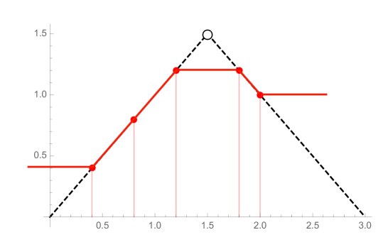
Figure 1: Conventional (solid line) vs. sparse (dashed line) piecewise-linear interpolants. The 5 data points are shown as red dots; they coincide with the knots of the conventional interpolant. The sparse solution, by contrast, has a single knot at $\tau_{1}=1.5$ (circle), an argument value that is found in none of the data points.

It is well known that the classical linear interpolator is the solution of the following variational problem, which we like to see as the precursor of RKHS kernel methods (Prenter, 1975; Wahba, 1990).

Proposition 2 (Sobolev optimality of piecewise-linear interpolation)

Let the native space be the first-order Sobolev space $H^{1}(\mathbb{R})=\{f:\mathbb{R}\to\mathbb{R}:\|{\rm D}f\|^{2}_{L_{2}}+|f(0)|^{2}<\infty\}$. Given a series of distinct data points $(x_{m},y_{m}),m=1,\dots,M$, the interpolation problem

$$\arg\min_{{f\in H^{1}(\mathbb{R})}}{\int_{\mathbb{R}}|{\rm D}f(x)|^{2}{\rm d}x}\mbox{ s.t. }\ f(x_{m})=y_{m},\ m=1,\dots,M$$

has a unique piecewise-linear solution that can be written as

$$s_{2}(x)=b_{1}+\sum_{m=1}^{M}a_{m}(x-x_{m})_{+}.$$ (11)

While the result is elegant and translates into a straightforward implementation, the scheme can be cumbersome for large data sets because the number of parameters in (11) increases with the number of data points. The other limitation is that the use of $\|{\rm D}f\|_{L_{2}}$-regularization disqualifies the simple linear solution $f(x)=ax$, which has an infinite cost.

As one may expect, there are also direct extensions of Lemma 1 and Proposition 2 for regularized least-squares approximations. Moreover, the distinction between the two types of solutions—smoothing splines (Schoenberg, 1964) vs. adaptive regression splines (Mammen and van de Geer, 1997)—is even more striking for noisy data fitting applications, which brings us back to our initial goal: the design and training of neural networks.

2.3 Representer theorem for deep neural networks

Our aim is to determine the optimal activation functions for a deep neural network in a task-dependent fashion. This problem is inherently ill-posed because activations are infinite-dimensional entities while we only have access to finite data. As in the case of interpolation, we resolve the ambiguity by imposing an appropriate form of regularization. Having singled out ${\rm TV}^{(2)}$ as the most favorable choice, we now proceed with the enunciation of our representer theorem for deep neural networks. We have purposefully stated the optimization problem in a generic form that is compatible with the current practice in DNN. Specifically, the cost function in (13) includes a standard data term that penalizes data misfit plus a regularization to constrain the values of the linear weights of the network (e.g., $R_{\ell}({\bf{U}}_{\ell})=\|{\bf{U}}_{\ell}\|^{2}_{\rm F}$ in the case of the popular weight-decay penalty). The novelty is the additional optimization over the neuronal activations $\sigma_{n,\ell}$ and the insertion of the ${\rm TV}^{(2)}$ term to regularize their shape.

Theorem 3 (${\rm TV}^{(2)}$-optimality of deep spline networks)

Let the $L$-layer feedforward neural network ${\bf{f}}:\mathbb{R}^{N_{0}}\to\mathbb{R}^{N_{L}}$ with node descriptor $(N_{0},N_{1},\dots,N_{L})$ take the form

$${\boldsymbol{x}}\mapsto{\bf{f}}({\boldsymbol{x}})=\left({\boldsymbol{\sigma}}_{L}\circ{\boldsymbol{\ell}}_{L}\circ{\boldsymbol{\sigma}}_{L-1}\circ\cdots\circ{\boldsymbol{\ell}}_{2}\circ{\boldsymbol{\sigma}}_{1}\circ{\boldsymbol{\ell}}_{1}\right)({\boldsymbol{x}}),$$ (12)

which is an alternating composition of the normalized linear transformations ${\boldsymbol{\ell}}_{\ell}:\mathbb{R}^{N_{\ell-1}}\to\mathbb{R}^{N_{\ell}},{\boldsymbol{x}}\mapsto{\bf{U}}_{\ell}{\boldsymbol{x}}$ with linear weights ${\bf{U}}_{\ell}=[{\bf{u}}_{1,\ell}\ \cdots\ {\bf{u}}_{N_{\ell},\ell}]^{T}\in\mathbb{R}^{N_{\ell}\times N_{\ell-1}}$ such that $\|{\bf{u}}_{n,\ell}\|=1$ and the nonlinear activations ${\boldsymbol{\sigma}}_{\ell}:\mathbb{R}^{N_{\ell}}\to\mathbb{R}^{N_{\ell}},{\boldsymbol{x}}\mapsto\big{(}\sigma_{1,\ell}(x_{1}),\dots,\sigma_{N_{\ell},\ell}(x_{n})\big{)}$ with $\sigma_{1,\ell},\dots,\sigma_{N_{\ell},\ell}\in{\rm BV}^{(2)}(\mathbb{R})$. Given a series of data points $({\boldsymbol{x}}_{m},{\boldsymbol{y}}_{m})_{m=1}^{M}$, we then define the training problem

$$\arg{\min_{({\bf{U}}_{\ell}),(\sigma_{n,\ell}\in{\rm BV}^{(2)}(\mathbb{R}))}}\left(\sum_{m=1}^{M}E\big{(}{\boldsymbol{y}}_{m},{\bf{f}}({\boldsymbol{x}}_{m})\big{)}\right.\left.+\mu\sum_{\ell=1}^{N}R_{\ell}({\bf{U}}_{\ell})+\lambda\sum_{\ell=1,}^{L}\sum_{n=1}^{N_{\ell}}{\rm TV}^{(2)}(\sigma_{n,\ell})\right)$$ (13)

where $E:\mathbb{R}^{N_{L}}\times\mathbb{R}^{N_{L}}\to\mathbb{R}^{+}$ is an arbitrary convex error function such that $E({\boldsymbol{y}},{\boldsymbol{y}})=0$ for any ${\boldsymbol{y}}\in\mathbb{R}^{N_{\ell}}$, $R_{\ell}:\mathbb{R}^{N_{\ell}\times N_{\ell}}\to\mathbb{R}^{+}$ is some arbitrary convex cost that favors certain types of linear transformations, and $\lambda,\mu\in\mathbb{R}^{+}$ are two adjustable regularization parameters. If the solution of (13) exists, then it is achieved by a deep spline network with individual activations of the form

$$\sigma_{n,\ell}(x)=b_{1,n,\ell}+b_{2,n,\ell}x+\sum_{k=1}^{K_{n,\ell}}a_{k,n,\ell}(x-\tau_{k,n,\ell})_{+},$$ (14)

with adaptive parameters $K_{n,\ell}\leq M-2$, $\tau_{1,n,\ell},\dots,\tau_{K_{n,\ell},n,\ell}\in\mathbb{R}$, and $b_{1,n,\ell},b_{2,n,\ell},a_{1,n,\ell}$, $\dots,a_{K_{n,\ell},n,\ell}\in\mathbb{R}$.

Proof  Let the function $\tilde{{\bf{f}}}:\mathbb{R}^{N_{0}}\to\mathbb{R}^{N_{L}}$ be a (not necessarily unique) solution of the problem summarized by (13). This solution is described by (12) with some optimal choice of transformation matrices $\tilde{{\bf{U}}}_{\ell}$ and pointwise nonlinearities $\tilde{\sigma}_{n,\ell}:\mathbb{R}\to\mathbb{R}$ for $\ell=1,\dots,L$ and $n=1,\dots,N_{\ell}$.

As we apply $\tilde{{\bf{f}}}$ to the data point ${\boldsymbol{x}}={\boldsymbol{x}}_{m}$ and progressively move through the layers of the network, we generate a series of vectors ${\boldsymbol{z}}_{m,\ell}\in\mathbb{R}^{N_{\ell}}$, according to the following recursive definition:

• Initialization (input of the network): $\tilde{{\boldsymbol{y}}}_{m,0}={\boldsymbol{x}}_{m}$.

• Recursive update: For $\ell=1,\dots,L$, calculate

  $${\boldsymbol{z}}_{m,\ell}=(z_{1,m,\ell},\dots,z_{N_{\ell},m,\ell})=\tilde{{\bf{U}}}_{\ell\,}\tilde{{\boldsymbol{y}}}_{m,\ell-1}$$ (15)

  and construct $\tilde{{\boldsymbol{y}}}_{m,\ell}=(\tilde{y}_{1,m,\ell},\dots,\tilde{y}_{N_{\ell},m,\ell})\in\mathbb{R}^{N_{\ell}}$ with

  $$\tilde{y}_{n,m,\ell}=\tilde{\sigma}_{n,\ell}(z_{n,m,\ell})\quad n=1,\dots,N_{\ell}.$$ (16)

At the output level, we get $\tilde{{\bf{f}}}({\boldsymbol{x}}_{m})=\tilde{{\boldsymbol{y}}}_{m,L}$ for $m=1,\dots,M$, which are the values that determine the data-fidelity part of the criterion associated with the optimal network and represented by the term $\sum_{m=1}^{M}E\big{(}{\boldsymbol{y}}_{m},{\bf{f}}({\boldsymbol{x}}_{m})\big{)}$ in (13). Likewise, the specification of the optimal linear transforms $\tilde{{\bf{U}}}_{1},\dots,\tilde{{\bf{U}}}_{L}$ fixes the regularization cost $\sum_{\ell=1}^{L}R_{\ell}({\bf{U}}_{\ell})$. Having set these quantities, we concentrate on the final element of the problem: the characterization of the “optimal” activations $\tilde{\sigma}_{n,\ell}:\mathbb{R}\to\mathbb{R}$ in-between the locations $z_{n,m,\ell}$ associated with the “auxiliary” data points $\tilde{y}_{n,m,\ell}=\tilde{\sigma}_{n,\ell}(z_{n,m,\ell})$, $m=1,\dots,M$. The key is to recognize that we can now consider the various activation functions individually because the variation of $\tilde{\sigma}_{n,\ell}$ in-between data points is entirely controlled by ${\rm TV}^{(2)}(\tilde{\sigma}_{n,\ell})$ without any influence on the other terms of the cost functional. Since the solution $\tilde{{\bf{f}}}$ achieves the global optimum, we therefore have that

$$\tilde{\sigma}_{n,\ell}=\arg\min_{f\in{\rm BV}^{(2)}(\mathbb{R})}\|{\rm D}^{2}f\|_{{\mathcal{M}}}\quad\mbox{ s.t. }\quad f(z_{n,m,\ell})=\tilde{y}_{n,m,\ell},\ \ m=1,\dots,M,$$

where the “auxiliary” data pairs $(z_{n,m,\ell},\tilde{y}_{n,m,\ell})$ are specified by (16). After this reformulation, we can apply Lemma 1, which proves that, at each node $(n,\ell)$, the minimum is achieved by a nonuniform spline with a number $K_{n,\ell}$ of knots smaller than the number of data points.

Since the hypothesis of feasibility is implicit in the construction, there is only one case not covered by Lemma 1: the singular scenario where all the auxiliary data points associated to a node are equal. Fortunately, this does not break the argument because such a configuration calls for a (zero-cost) solution of the form $b_{1}+b_{2}x$ (which is a special case of (10) with $K=0$), except for the twist that there are now infinitely many possibilities with $b_{1}+b_{2}z_{1}=\tilde{y}_{1}$.

 

This result translates into a computational structure where each node of the network (with fixed index $(n,\ell)$) is characterized by

• its number $0\leq K=K_{n,\ell}$ of knots (ideally, much smaller than $M$);

• the location $\{\tau_{k}=\tau_{k,n,\ell}\}_{k=1}^{K_{n,\ell}}$ of these knots (equivalent to ReLU biases);

• the expansion coefficients $b_{1,n,\ell},b_{2,n,\ell},a_{1,n,\ell},\ldots,a_{K,n,\ell}$, also written as ${\bf{b}}=(b_{1},b_{2})\in\mathbb{R}^{2}$ and ${\bf{a}}=(a_{1},\ldots,a_{K})\in\mathbb{R}^{K}$ to avoid notational overload.

The fundamental point is that these parameters (including the number of knots) are data-dependent and adjusted automatically through the minimization of (13). All this takes place during training.

3 Interpretation and discussion

Theorem 3 tells us that we can configure a neural network optimally by restricting our attention to piecewise-linear activation functions $\sigma_{n,\ell}$, or spline activations, for short. In effect, this means that the “infinite-dimensional” minimization problem specified by (13) can be converted into a tractable finite-dimensional problem where, for each node $(n,\ell)$, the parameters to be optimized are the number $K_{n,\ell}$ of knots, the locations $\{\tau_{k,n,\ell}\}_{k=1}^{K_{n,\ell}}$ of the spline knots, and the linear weights $b_{1,n,\ell},b_{2,n,\ell},a_{1,n,\ell},\dots,$ $a_{K_{n,\ell},n,\ell}\in\mathbb{R}$. The enabling property is going to be (19), which converts the continuous-domain regularization into a discrete $\ell_{1}$-norm. This is consistent with the expectation that bounding the second-order total-variation favors solutions with sparse second derivatives—i.e., linear splines with the fewest possible number of knots. The idea is that $\ell_{1}$-minimization helps reducing the number of active coefficients $a_{k,n,\ell}$ (Donoho, 2006; Unser et al., 2016).

The other important feature is that the knots are adaptive and that they can be learned during training using the standard backpropagation algorithm. What is required is the derivative of the activation functions. It is given by

$$\sigma^{\prime}_{n,\ell}(x)=b_{2,n,\ell}+\sum_{k=1}^{K_{n,\ell}}a_{k,n,\ell}\mathbbm{1}_{[\tau_{k,n,\ell},+\infty)}(x),$$ (17)

where $\mathbbm{1}_{[\tau,+\infty)}(x)$ is an indicator function that is zero for $x<\tau$ and $1$ otherwise. These derivatives are piecewise-constant splines with jumps of height $a_{k,n,\ell}$ at the knot locations $\tau_{k,n,\ell}$. By differentiating (17) once more, we get

$$\sigma^{\prime\prime}_{n,\ell}(x)=\sum_{k=1}^{K_{n,\ell}}a_{k,n,\ell}\delta(x-\tau_{k,n,\ell}),$$ (18)

where $\delta$ is the Dirac distribution. Owing to the property that $\|\delta(\cdot-\tau_{k,n,\ell})\|_{{\mathcal{M}}}=1$, we then readily deduce that

$${\rm TV}^{(2)}\{\sigma_{n,\ell}\}=\|\sigma^{\prime\prime}_{n,\ell}\|_{{\mathcal{M}}}=\sum_{k=1}^{K_{n,\ell}}|a_{k,n,\ell}|=\|{\bf{a}}_{n,\ell}\|_{1},$$ (19)

which converts the continuous-domain regularization into a more familiar minimum $\ell_{1}$-norm constraint on the underlying expansion coefficients.

3.1 Link with existing techniques

What is even more interesting, from a practical point of view, is that the corresponding system translates into a deep ReLU network modulo a slight modification of the standard architecture described by (6). Indeed, the primary basis functions in (14) are shifted ReLUs, so that each spline activation $\sigma_{n,\ell}$ can be realized by way of a simple one-layer ReLU subnetwork with the spline knots being encoded in the biases. In particular, when the only active coefficients is $a_{n,\ell}\stackrel{{\scriptstyle\vartriangle}}{{=}}a_{1,n,\ell}$ (i.e., $b_{1,n,\ell}=0$, $b_{2,n,\ell}=0$, and $K_{n,\ell}=1$), we have a perfect equivalence with the classical deep ReLU structure described by (6) with $\sigma_{n,\ell}(x)=(x)_{+}$. The enabling property is that

$$({\bf{w}}^{T}_{n,\ell}{\boldsymbol{x}}-z_{n,\ell})_{+}=(a_{n,\ell}{\bf{u}}^{T}_{n,\ell}{\boldsymbol{x}}-z_{n,\ell})_{+}=a_{n,\ell}({\bf{u}}^{T}_{n,\ell}{\boldsymbol{x}}-\tau_{n,\ell})_{+},$$

with ${\bf{u}}_{n,\ell}={\bf{w}}_{n,\ell}/\|{\bf{w}}_{n,\ell}\|$, $a_{n,\ell}=\|{\bf{w}}_{n,\ell}\|$ and $\tau_{n,\ell}=z_{n,\ell}/a_{n,\ell}$. Concretely, this means that, for every layer $\ell$, we can absorb the single ReLU coefficients $a_{n,\ell},n=1,\dots,N_{\ell}$ into the prior linear transformation and consider unnormalized transformations ${\bf{W}}_{\ell}=[{\bf{w}}_{1,\ell}\ \dots\ {\bf{w}}_{N_{\ell}},]^{T}$ (as in (4)) rather than the normalized ones of Theorem 3 with ${\bf{u}}_{n,\ell}={\bf{w}}_{n,\ell}/\|{\bf{w}}_{n,\ell}\|$.

Theorem 3 then suggests that the next step in complexity is to add the linear term $b_{1,n,\ell}+b_{2,n,\ell}x$ to each node, since its regularization cost vanishes. Interestingly, the suggested configuration—that is, one ReLU plus an adjustable linear term per neuron—is equivalent to the parametric ReLU model (PReLU) of He et al. (2015), which has been found to systematically outperform the baseline ReLU configuration in real-world applications. The other design extreme is to let $\lambda\to\infty$, in which case the whole network collapses, leading to an affine mapping of the form ${\bf{f}}({\boldsymbol{x}})={\bf{W}}{\boldsymbol{x}}-{\bf{b}}$ with ${\bf{W}}\in\mathbb{R}^{N_{L}\times N_{0}}$ and ${\bf{b}}\in\mathbb{R}^{N_{L}}$. More generally, the framework provides us with the possibility of controlling the number of knots (and hence the complexity of the network) through the simple adjustment of the regularization parameter $\lambda$, with the number of knots increasing as $\lambda\to 0$.

Among the various attempts in the literature to optimize the shape of the activation functions in deep neural networks, there is one scheme that is remarkably close to the optimal solution suggested by our theorem: the APL (adaptive piecewise-linear activation) framework of Agostinelli et al. (2015) in which each neuron is represented as a linear combination of shifted ReLUs, with the parameter being determined during training. The only difference is that their number of ReLUs is fixed a priori and that their model does not include the linear term $b_{1}+b_{2}x$. While Agostinelli et al.’s formulation does not involve any explicit regularization, they found in their experiments that is was helpful to add some mild $\ell_{2}$ penalty on the ReLU coefficients (to be contrasted with the sparsity-promoting $\ell_{1}$-penalty that results from our theorem) to avoid numerical instability. The good news in support of our theorem is that they report substantial improvement (9.4% and 7.5% relative error decrease, respectively) on state-of-the-art CNN (with fixed RELU activations) on the CIFAR-10 and CIFAR-100 classification benchmarks.

A characteristic property of deep spline networks, to be considered here as a superset of the traditional deep ReLU networks, is that they produce an input-output relation that is continuous and piecewise-linear (CPWL) in the following sense: the corresponding function ${\bf{f}}$ is continuous $\mathbb{R}^{N_{0}}\to\mathbb{R}^{N_{L}}$; its domain $\mathbb{R}^{N_{0}}=\bigcup_{k=1}^{K}P_{k}$ can be partitioned into a finite set of non-overlapping convex polytopes $P_{k}$ over which it is affine (Tarela and Martinez, 1999; Wang and Sun, 2005). More precisely, ${\bf{f}}({\boldsymbol{x}})={\boldsymbol{f}}_{k}({\boldsymbol{x}})$ for all ${\boldsymbol{x}}\in P_{k}$ where ${\boldsymbol{f}}_{k}:\mathbb{R}^{N_{0}}\to\mathbb{R}^{N_{L}}$ has the same parametric form as in (4) . This simply follows from the observation that ${\boldsymbol{\sigma}}_{\ell}=(\sigma_{1,\ell},\dots,\sigma_{N_{\ell},\ell})$, with $\sigma_{n,\ell}$ as specified by (14), is CPWL and that the CPWL property is conserved through functional composition. In fact, the CPWL property for $N=1$ is equivalent to the function being a nonuniform spline of degree 1.

Another powerful architecture that is known to generate CPWL functions is the MaxOut network (Goodfellow et al., 2013). There, the non-linear steps ${\boldsymbol{\sigma}}_{\ell}$ in (6) are replaced by max-pooling operations. It turns out that these operations are also expressible in terms of deep splines, as illustrated in Figure 2 for the simple case where the maximum is taken over two inputs. Interestingly, this conversion requires the use of the linear term which is absent in conventional ReLU networks. This reinforces the argument made by Goodfellow et al. concerning the capability of MaxOut to learn activation functions.

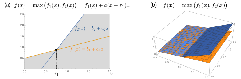
Figure 2: Deep-spline implementation of MaxOut with $N=2$. (a) In one dimension, the spline parameters are $a=(a_{2}-a_{1})$ and $\tau_{1}=(b_{2}-b_{1})/(a_{2}-a_{1})$. (b) In two or more dimensions, $f({\boldsymbol{x}})=b_{1}+{\boldsymbol{a}}_{1}^{T}{\boldsymbol{x}}+a({\boldsymbol{u}}^{T}{\boldsymbol{x}}-\tau_{1})_{+}$, where ${\boldsymbol{u}}$ is the unit vector perpendicular to the hinge.

An attractive feature that is offered by the deep-spline parameterization is the possibility of suppressing a network layer—or rather, merging two adjacent ones—when the optimal solution is such that $K_{n,\ell}=0$ for $\ell$ fixed and $n=1,\dots,N_{\ell}$. This is a property that results from the presence of the linear component and has not been exploited so far.

3.2 Generalizations

The optimality result in Theorem 3 holds for a remarkably broad family of cost functions, which should cover all cases of practical interest. The first condition is that the data term, as its name suggest, be solely dependent on ${\boldsymbol{y}}_{m}$ and ${\boldsymbol{f}}({\boldsymbol{x}}_{m})$. The second is that the regularization of the weights—the part that constrains the linear steps—and the regularization of the individual activation functions are decoupled from each others. Obvious generalizations of the result include

• cases where the optimization in (13) is performed over a subset of the components while other network elements such as critical linear weights, activation functions or even pooling operators are fixed beforehand; in particular, this includes the important subclass of networks that are not fully connected;

• configurations such as those found in convolutional networks where some (tunable) activation functions are shared among multiple nodes;

• generalized forms of regularization where ${\rm TV}^{(2)}(\sigma_{n,\ell})$ is substituted by $\psi\big{(}{\rm TV}^{(2)}(\sigma_{n,\ell})\big{)}$, where $\psi:\mathbb{R}^{+}\to\mathbb{R}^{+}$ is any monotonically increasing function.

While the first and second scenarios require a slight reformulation of the optimization problem, it is still possible to invoke the same kind of “interpolation” argument as in the proof of Theorem 3. The third generalization is obvious since the (constrained) miminization of ${\rm TV}^{(2)}(\sigma_{n,\ell})$ is equivalent to the minimization of $\psi\big{(}{\rm TV}^{(2)}(\sigma_{n,\ell})\big{)}$.

The statement in Theorem 3 refers to the global optimum of (13), which is often hard to reach in practice (because the underlying problem is highly non-convex). It turns out that the argument of the proof is also applicable to local minima and/or saddle points of the cost functional.

By relying on the supporting mathematics in Appendix B for general spline-admissible operators ${\rm L}$, it is possible to revisit the proof of Theorem 3 to determine the parametric form of the optimal activations for higher-order versions of TV regularization; i.e., ${\rm TV}^{(n)}(\sigma)=\|{\rm D}^{n}\sigma\|_{{\mathcal{M}}}$. This yields optimal activations that are non-uniform polynomial splines of degree $n>2$. While such solutions have a higher-order of differentiability, they are less favourable globally because the underlying spline property is not retained through composition, meaning that the larger the number of layers, the larger the polynomal degree of the “polytopes” of the resulting network. By contrast, the CPWL property of the linear splines in (14) is preserved through composition, so that the resulting deep spline DNN can be also be interpreted as a flat (or shallow) multidimensional piecewise-linear spline. The other way of inducing CPWL activations is through the quadratic Sobolev 1 regularization of Proposition 2. However, this solution has two shortcommings: (i) its inability to represent the identity which would result in an infinite cost, and (ii) its lack of sparsity.

3.3 Comparison with kernel methods

We like to contrast the result in Theorem 3 with the classical representer theorem of machine learning (Schölkopf et al., 2001). The commonality is that both theorems provide a parametric representation of the solution in the form of a linear “kernel” expansion. The primary distinction is that the classical representer theorem is restricted to “shallow” networks with $L=1$. Yet, there is another difference even more crucial for our purpose: the fact that the knots $\tau_{k}$ in (14) are adaptive and few ($K\ll M)$, while the centers ${\boldsymbol{x}}_{m}$ in (2) are fixed and as numerous as there are data points in the training set. In addition, the ReLU function $(x)_{+}$ is not a kernel in the traditional sense of the term because it is not positive-definite. We note, however, that it can be substituted by another equivalent spline generator $|x|$, which is conditionally positive-definite (Micchelli, 1986; Wendland, 2005). Again, the property that makes this feasible is the presence of the linear term $b_{1,n,\ell}+b_{2,n,\ell}x$.

There is also a conceptual similarity between the result of Theorem 3 and a recent representer theorem for deep kernel networks (Bohn et al., 2018), which results in a solution that is a composition of $L$ multi-valued kernel estimators of the classical RKHS form given by (2). Again, the two main differences with the present framework are: (i) each layer of the deep kernel network is a multivariate non-linear map, which does not necessarily allow for affine transformations (e.g. linear regressions) and, (ii) the kernel expansion in each layer requires as many basis functions as there are training data; this amounts to a total of $L\times M$ linear parameters—this can rapidly become prohibitive, not to mention the complexity of the underlying (non-convex) optimization task. The first shortcoming can easily be fixed by inserting intermediate affine transformations in direct analogy with the type of architecture covered by Theorem 3. The second limitation is more fundamental and can probably only be removed by adopting some kind of generalized TV regularization in the spirit of Unser et al. (2017); in short, this calls for an extension of Theorem 3 for multivariate activations, which is currently work in progress.

3.4 Towards a practical implementation

While the solution of Theorem 3 is conceptually appealing, it can be expected to be harder to implement than fixed kernel/RKHS methods since the optimization is not only over the linear weights ${\boldsymbol{a}}_{n,\ell}$ and ${\boldsymbol{b}}_{n,\ell}$, but also over the number and positions of the corresponding spline knots. There is also always a risk that an increase in the number of degrees of freedom may compromise the generalization ability of the result network, which means that the method will need to be carefully tested and validated on real data. A possible strategy for making the optimization easier is to constrain the ReLU units to lie on a grid—in the spirit of Gupta et al. (2018)—and to then rely on standard iterative $\ell_{1}$-norm minimization techniques to produce a sparse solution (Donoho, 2006; Foucart and Rauhut, 2013; Unser et al., 2016). Such a scheme may still require some explicit knot-deletion step, either as post-processing or during the training iterations, to effectively trim down the number of parameters. A potential difficulty is that minimum ${\rm TV}^{(2)}$ interpolants are typically non-unique, because the underlying regularization is semi-convex. This means that the solution found by an iterative algorithm—assuming that the minimum of the regularization energy is achieved—is not necessarily the sparsest one within the (convex) solution set. Designing an algorithm that can effectively deal with this issue will be a very valuable contribution to the field.

4 Conclusion

The main contribution of this work is to provide the theoretical foundations for an integrated approach to neural networks where a sub-part of the design—the optimal shaping of activations—can be transferred to the training part of the process and formulated as a global optimization problem. It also deepens the connection between splines and multilayer ReLU networks, as a pleasing side product. While the concept seems promising and includes the theoretical possibility of suppressing unnecessary layers, it raises a number of issues that can only be answered through extensive experimentation with real data. There are already strong indications in the literature (e.g., the improved performance of PReLU) of the practical usefulness of the linear-activation component that is suggested by the theory and not present in traditional ReLU systems. The next task ahead is to demonstrate the capability of more complex spline activations to improve upon the state-of-the-art. (Except for a potential risk of over-parameterization, deep-spline networks should perform at least as well as deep ReLU, PReLU or APL networks since the latter constitute a subset of the former.)

We expect the greatest challenge for training a deep spline network to be the proper optimization of the number of knots at each neuron, given that the solution with the fewest parameters is the most desirable. In short, we are still in need of a practical and efficient solution for training a deep neural network with fully adaptable activations that globally produces a continuous and piecewise-linear input-output relation; in other words, a DNN that implements an adaptive multidimensional linear spline.

Appendices

The proof of Lemma 1 is based on some foundational results in (Unser et al., 2017) that rely on compactness arguments requiring the weak* topology. We therefore start with a brief review of the relevant notions from functional analysis (Appendix A). We then specify the topology of ${\rm BV}^{(2)}(\mathbb{R})$ in Appendix B and precisely delineate its predual space in Theorem 10. This latter characterization is the key to the proof of Lemma 1 that is presented in Appendix C.

A Background on continuity and weak* continuity

Definition 4

Let $v:u\mapsto\langle v,u\rangle$ be a linear functional on a Banach space ${\mathcal{U}}$ equipped with the norm $\|\cdot\|_{{\mathcal{U}}}$. Then, $v:{\mathcal{U}}\to\mathbb{R}$ is said to be continuous if $\ \lim_{n\to\infty}\langle v,u_{n}\rangle=\langle v,u\rangle$ for any sequence $(u_{n})$ in ${\mathcal{U}}$ such that $\lim_{n\to\infty}\|u_{n}-u\|_{{\mathcal{U}}}=0$.

We recall that ${\mathcal{U}}^{\prime}$ (the continuous dual of ${\mathcal{U}}$) is the vector space that is formed of the linear functionals that are continuous on ${\mathcal{U}}$; it is a Banach space equipped with the dual norm

$$\|v\|_{{\mathcal{U}}^{\prime}}=\sup_{\varphi\in{\mathcal{U}}:\|u\|_{{\mathcal{X}}}\leq 1}\langle v,u\rangle.$$

By following up on the above property, one specifies the space of linear functionals that are continuous on ${\mathcal{U}}^{\prime}$, which yields the Banach space ${\mathcal{U}}^{\prime\prime}$. A standard result in functional analysis is that ${\mathcal{U}}$ is continuously embedded in its bidual ${\mathcal{U}}^{\prime\prime}$, which is indicated as ${\mathcal{U}}\xhookrightarrow{}{\mathcal{U}}^{\prime\prime}$, with the two spaces being isometrically isomorphic (i.e., ${\mathcal{U}}={\mathcal{U}}^{\prime\prime}$) if and only if ${\mathcal{U}}$ is reflexive (Rudin, 1991). In other words, the construction of the bidual ${\mathcal{U}}^{\prime\prime}$ gets us back to the initial space in the reflexive case only.

A primary case of interest for this paper is $\ {\mathcal{U}}^{\prime}={\mathcal{M}}(\mathbb{R})$ which is not reflexive. For such a scenario, the proper way to deduce the predual space ${\mathcal{U}}$ from ${\mathcal{V}}={\mathcal{U}}^{\prime}$ is through the identification of the linear functionals that are weak*-continuous on ${\mathcal{V}}$.

Definition 5 (Weak* topology)

A sequence $(v_{n})_{n=1}^{\infty}$ in ${\mathcal{V}}={\mathcal{U}}^{\prime}$ is said to converge to $v$ in the weak* topology if $\lim_{n\to\infty}\langle v_{n}-v,u\rangle=0\$ for all $u\in{\mathcal{U}}$.

Definition 6 (weak* continuity)

A linear functional $u:{\mathcal{U}}^{\prime}\to\mathbb{R}$ is said to be weak*-continuous if $\ \lim_{n\to\infty}\langle u,v_{n}\rangle=\langle u,v\rangle$ for any sequence $(v_{n})$ that converges to $v$ in the weak* topology.

Proposition 7 (see (Reed and Simon, 1980, Theorem IV.20, p. 114))

The only weak* continuous linear functionals on ${\mathcal{U}}^{\prime}$ are the elements of ${\mathcal{U}}$.

The main point is that, despite the qualifier “weak”, the functional property of weak* continuity is actually stricter than continuity.

In practice, it is relatively straightforward to establish the continuity of $u:{\mathcal{V}}\to\mathbb{R}$ since the property is equivalent to the existence of a constant $C>0$ such

$$|\langle u,v\rangle|\leq C\|v\|_{{\mathcal{V}}}$$

for all $v\in{\mathcal{V}}$, which also yields $\|u\|_{{\mathcal{V}}^{\prime}}\leq C<\infty$. By contrast, proving that $v:{\mathcal{V}}\to\mathbb{R}$ is weak*-continuous in the non-reflexive scenario requires the precise characterization of the predual of ${\mathcal{V}}$, which is typically more demanding mathematically. For instance, the property that ${\mathcal{M}}(\mathbb{R})=\big{(}C_{0}(\mathbb{R})\big{)}^{\prime}$ is a fundamental result in measure theory known as the Riesz-Markov theorem (Rudin, 1987).

For example, the functionals $\varphi\mapsto\langle 1,\varphi\rangle$ and $\varphi\mapsto\langle\mathbbm{1}_{[0,1]},\varphi\rangle$ are continuous on ${\mathcal{M}}(\mathbb{R})=\big{(}C_{0}(\mathbb{R})\big{)}^{\prime}$ because the “generalized” functions $1$ and $\mathbbm{1}_{[0,1]}$ are bounded in the $\sup$-norm. However, they both fail to be weak*-continuous; i.e., $1\notin C_{0}(\mathbb{R})$ because it does not decay at infinity, and $\mathbbm{1}_{[0,1]}\notin C_{0}(\mathbb{R})$ because it is not continuous everywhere. In the latter example, we may recover weak* continuity by considering a smoothed version of the indicator function.

These considerations are central to the proof of Lemma 1 because it requires the weak* continuity of the sampling functional $\delta(\cdot-x_{m})$. While the sampling operation is continuous on ${\rm BV}^{(2)}(\mathbb{R})$, it is not necessarily weak*-continuous; at least not in the canonical topology that is proposed in (Unser et al., 2017, p. 780) (e.g., polynomial spline example with $N_{0}=2$ and ${\boldsymbol{\phi}}=(\delta,-\delta^{\prime})$). This is the reason why we need to revisit the construction of our native space, as detailed in Appendix B, and establish a new operational criterion for testing weak* continuity (Theorem 10).

B Banach structure of ${\rm BV}^{(2)}(\mathbb{R})$ and of its predual space

While the definition of ${\rm BV}^{(2)}(\mathbb{R})$ given in (8) is convenient for expository purposes, it is not directly usable for mathematical analysis because the functional $\|{\rm D}^{2}f\|_{{\mathcal{M}}}$ is only a semi-norm. To lift the ambiguity due to the non-trivial null space, we select a biorthogonal system $({\boldsymbol{\phi}},{\boldsymbol{p}})$ for ${\mathcal{N}}_{{\rm D}^{2}}$ (the null space of ${\rm D}^{2}$). In order to fix the problem of weak* continuity (see explanations surounding Figure 3), our proposed modification of the canonical scheme is ${\boldsymbol{\phi}}=(\phi_{1},\phi_{2})=\big{(}\delta,-\delta+\delta(\cdot-1)\big{)}$ and ${\boldsymbol{p}}=(p_{1},p_{2})$, with $p_{1}(x)=1$ and $p_{2}(x)=x$, which are such that $\langle p_{1},\phi_{1}\rangle=p_{1}(0)=1$, $\langle p_{1},\phi_{2}\rangle=-p_{1}(0)+p_{1}(1)=0$, $\langle p_{2},\phi_{1}\rangle=p_{2}(0)=0$ and $\langle p_{2},\phi_{2}\rangle=-p_{2}(0)+p_{2}(1)=1$ (biorthogonality property). We then rely on (Unser et al., 2017, Theorem 5) to get the following characterization.

Proposition 8 (Banach structure of ${\rm BV}^{(2)}(\mathbb{R})$)

Let $({\boldsymbol{\phi}},{\boldsymbol{p}})$ be a biorthogonal system for ${\mathcal{N}}_{{\rm D}^{2}}={\rm span}\{1,x\}$. Then, ${\rm BV}^{(2)}(\mathbb{R})$ equipped with the norm

$$\|f\|=\|{\rm D}^{2}f\|_{{\mathcal{M}}}+\sqrt{|\langle\phi_{1},f\rangle|^{2}+|\langle\phi_{2},f\rangle|^{2}},$$

is a (non-reflexive) Banach space. Moreover, every $f\in{\rm BV}^{(2)}(\mathbb{R})$ has the unique direct-sum decomposition

$$f={\mathrm{G}}_{\boldsymbol{\phi}}\{w\}+p,$$ (20)

where $w={\rm D}^{2}f\in{\mathcal{M}}(\mathbb{R})$, $p=\sum_{n=1}^{2}\langle f,\phi_{n}\rangle p_{n}\in{\mathcal{N}}_{{\rm D}^{2}}$, and ${\mathrm{G}}_{\boldsymbol{\phi}}:w\mapsto\int_{\mathbb{R}}g_{{\boldsymbol{\phi}}}(\cdot,y)w(y){\rm d}y$, with

$$g_{{\boldsymbol{\phi}}}(x,y) =(x-y)_{+}-p_{1}(x)\langle\phi_{1},(\cdot-y)_{+}\rangle-p_{2}(x)\langle\phi_{2},(\cdot-y)_{+}\rangle.$$ (21)

Central to our formulation is the unique operator ${\mathrm{G}}_{\boldsymbol{\phi}}:{\mathcal{M}}(\mathbb{R})\to{\rm BV}^{(2)}(\mathbb{R})$ such that

$${\rm D}^{2}{\mathrm{G}}_{\boldsymbol{\phi}}\{w\}=w \qquad(\mbox{right-inverse property})$$ (22)

$$\langle\phi_{1},{\mathrm{G}}_{{\boldsymbol{\phi}}}\{w\}\rangle=0,\quad\langle\phi_{2},{\mathrm{G}}_{\boldsymbol{\phi}}\{w\}\rangle=0 \qquad(\mbox{boundary conditions})$$ (23)

for all $w\in{\mathcal{M}}(\mathbb{R})$. Specifically, (23) ensures the orthogonality of the two components of the direct sum decomposition of $f$ in (20), while (22) and the biorthogonality of $({\boldsymbol{\phi}},{\boldsymbol{p}})$ guarantees its unicity.

By fixing $\phi_{1}=\delta$ and $\phi_{2}=-\delta+\delta(\cdot-1)$ (finite difference), we obtain the formula of the norm for ${\rm BV}^{(2)}(\mathbb{R})$ given by (9). The corresponding expression of the kernel of ${\mathrm{G}}_{\boldsymbol{\phi}}$ given by (21) is

$$g_{{\boldsymbol{\phi}}}(x,y) =(x-y)_{+}-(1-x)(-y)_{+}-x(1-y)_{+}.$$ (24)

A crucial observation for the proof of Lemma 1 is that the function $y\mapsto g_{{\boldsymbol{\phi}}}(x,y)$ specified by (24) is compactly supported and bounded—in contrast with the leading term of the expansion $(x-y)_{+}$ in (21), which represents the impulse response of the conventional shift-invariant inverse of ${\rm D}^{2}$ (two-fold integrator). In fact, these functions are continuous, triangle-shaped B-splines with the following characteristics (see Figure 3).

• for $x\leq 0$: $y\mapsto g_{{\boldsymbol{\phi}}}(x,y)$ is supported in $[x,1]$ and takes its maximum at $y=0$

• for $x\in(0,1)$: $y\mapsto g_{{\boldsymbol{\phi}}}(x,y)$ is supported in $[0,1]$ and takes its extremum at $y=x$

• for $x\geq 1$: $y\mapsto g_{{\boldsymbol{\phi}}}(x,y)$ is supported in $[0,x]$ and takes its maximum at $y=1$.

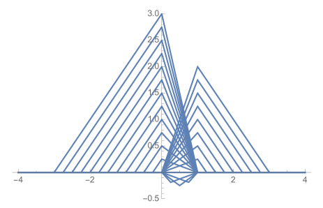
Figure 3: Graphs of the function $y\mapsto g_{{\boldsymbol{\phi}}}(x,y)$ for a series of values of $x=-3,\dots,3$ with steps of $0.25$. This illustrates the property that $g_{{\boldsymbol{\phi}}}(x,\cdot)\in C_{0}(\mathbb{R})$ for any $x\in\mathbb{R}$, which is critical to the proof of Lemma 1. By contrast, the canonical solution of (Unser et al., 2017) with ${\boldsymbol{\phi}}=(\delta,-\delta^{\prime})$ would have resulted in a series of piecewice-linear functions with a discontinuous drop to $0$ at $x=0$.

Since ${\rm BV}^{(2)}(\mathbb{R})$ is non-reflexive, the characterization of its predual is required for testing the hypothesis of weak* continuity. To that end, we first recall that the predual of ${\mathcal{M}}(\mathbb{R})=\big{(}C_{0}(\mathbb{R})\big{)}^{\prime}$ is the space $C_{0}(\mathbb{R})$ of continuous functions that vanish at infinity equipped with the sup norm (Rudin, 1987). Moreover, since ${\mathcal{S}}(\mathbb{R})$ (Schwartz’ space of smooth and rapidly-decaying functions) is dense in $C_{0}(\mathbb{R})$ (Schwartz, 1966), the latter can also be described as the completion of ${\mathcal{S}}(\mathbb{R})$ equipped with the sup norm, in conformity with the definition of ${\mathcal{M}}(\mathbb{R})$ given by (7).

We now present an explicit construction and characterization of the predual of ${\rm BV}^{(2)}(\mathbb{R})$. This description is consistent with an earlier theorem of ours (Unser et al., 2017, Theorem 6) applicable to general spline spaces; however, it contributes two novel elements: (i) the operational criterion for space membership provided by the first property, and (ii) the construction of the predual space $C_{{\rm D}^{2},{\boldsymbol{\phi}}}(\mathbb{R})$ via the completion of ${\mathcal{S}}(\mathbb{R})$, which requires additional hypotheses on ${\boldsymbol{\phi}}$.

Definition 9

Let ${\boldsymbol{p}}=(p_{1},p_{2})$ be a basis of ${\mathcal{N}}_{{\rm D}^{2}}={\rm span}\{1,x\}$ and ${\boldsymbol{\phi}}=(\phi_{1},\phi_{2})$ a complementary set of (generalized) functions whose Fourier transforms are denoted by $\widehat{\phi}_{1},\widehat{\phi}_{2}$. Then, the system $({\boldsymbol{p}},{\boldsymbol{\phi}})$ is said to be admissible for ${\rm D}^{2}$ if

1. the basis functions are biorthogonal; i.e., $\langle\phi_{m},p_{n}\rangle=\delta_{m,n},\ (m,n=1,2)$

2. $\widehat{\phi}_{1},\widehat{\phi}_{2}\in L_{1,2}(\mathbb{R})=\{f:\mathbb{R}\mapsto\mathbb{R}\ \ \big{|}\ \int_{\mathbb{R}}(1+|\omega|)^{-2}|f(\omega)|{\rm d}\omega<\infty\}$ with the two functions being continuously differentiable twice at $\omega=0$.
   

Theorem 10 (Predual of native space)

Let $({\boldsymbol{\phi}},{\boldsymbol{p}})$ be an admissible system in the sense of Definition 9. Then, the function space

$$C_{{\rm D}^{2},{\boldsymbol{\phi}}}(\mathbb{R})=\{g={\rm D}^{2}v+a_{1}\phi_{1}+a_{2}\phi_{2}:v\in C_{0}(\mathbb{R}),{\boldsymbol{a}}=(a_{1},a_{2})\in\mathbb{R}^{2}\}$$ (25)

has the following properties:

1. every $g\in C_{{\rm D}^{2},{\boldsymbol{\phi}}}(\mathbb{R})$ has a unique direct-sum representation as in (25) with $v={\mathrm{G}}^{\ast}_{\boldsymbol{\phi}}\{g\}$, $a_{1}=\langle p_{1},g\rangle$, and $a_{2}=\langle p_{2},g\rangle$, where ${\mathrm{G}}^{\ast}_{\boldsymbol{\phi}}$ is the adjoint of ${\mathrm{G}}_{\boldsymbol{\phi}}$ specified by (21);

2. $C_{{\rm D}^{2},{\boldsymbol{\phi}}}(\mathbb{R})$ is a (non-reflexive) Banach space equipped with the norm

   $$\|g\|_{C_{{\rm D}^{2},{\boldsymbol{\phi}}}}\stackrel{{\scriptstyle\vartriangle}}{{=}}\|{\mathrm{G}}^{\ast}_{\boldsymbol{\phi}}g\|_{\infty}+\|{\boldsymbol{p}}(g)\|_{2}=\|v\|_{\infty}+\|{\boldsymbol{a}}\|_{2};$$ (26)

3. $C_{{\rm D}^{2},{\boldsymbol{\phi}}}(\mathbb{R})$ is the predual of ${\rm BV}^{(2)}(\mathbb{R})$ in Proposition 8; i.e., ${\rm BV}^{(2)}(\mathbb{R})=\big{(}C_{{\rm D}^{2},{\boldsymbol{\phi}}}(\mathbb{R})\big{)}^{\prime}$;

4. $C_{{\rm D}^{2},{\boldsymbol{\phi}}}(\mathbb{R})$ is the completion of ${\mathcal{S}}(\mathbb{R})$ equipped with the $\|\cdot\|_{C_{{\rm D}^{2},{\boldsymbol{\phi}}}}$-norm.

Proof : The main idea is that the construction expressed by (25) is the direct sum of two linear spaces, ${\mathcal{U}}$ and ${\mathcal{N}}_{{\boldsymbol{\phi}}}$, whose Banach topology and completion properties are revealed next.
(i): Topology of the space ${\mathcal{N}}_{{\boldsymbol{\phi}}}={\rm span}\{\phi_{1},\phi_{2}\}$ and of its dual
This space collects the two last components of $g$ in (25) and is equipped with the discrete $\ell_{2}$-norm $\|\phi\|_{{\mathcal{N}}_{{\boldsymbol{\phi}}}}=\|{\bf{a}}\|_{2}$ with ${\bf{a}}={\boldsymbol{p}}(\phi)=(\langle p_{1},\phi\rangle,\langle p_{2},\phi\rangle)$. We also specify the projection operator $C_{{\rm D}^{2},{\boldsymbol{\phi}}}(\mathbb{R})\to{\mathcal{N}}_{{\boldsymbol{\phi}}}$:

$${\rm Proj}_{{\mathcal{N}}_{{\boldsymbol{\phi}}}}\{g\}=\langle p_{1},g\rangle\phi_{1}+\langle p_{2},g\rangle\phi_{2}.$$

The complementary space is ${\mathcal{N}}_{{\boldsymbol{p}}}\stackrel{{\scriptstyle\vartriangle}}{{=}}{\rm span}\{p_{1},p_{2}\}$ equipped with the norm $\|p\|_{{\mathcal{N}}_{{\boldsymbol{p}}}}=\|{\boldsymbol{p}}(p)\|_{2}=\|{\bf{b}}\|_{2}$ with ${\bf{b}}={\boldsymbol{\phi}}(p)=(\langle\phi_{1},p\rangle,\langle\phi_{2},p\rangle)$. Thanks to the biorthogonality of ${\boldsymbol{\phi}}$ and ${\boldsymbol{p}}$, for all $p={b_{1}p_{1}+b_{2}p_{2}}\in{\mathcal{N}}_{{\boldsymbol{p}}}$, we have that

$$\|p\|_{{\mathcal{N}}^{\prime}_{{\boldsymbol{\phi}}}}=\sup_{\phi\in{\mathcal{N}}_{{\boldsymbol{\phi}}}:\|\phi\|_{{\mathcal{N}}_{{\boldsymbol{\phi}}}}\leq 1}\langle\phi,p\rangle=\sup_{{\bf{a}}\in\mathbb{R}^{2}:\|{\bf{a}}\|_{2}\leq 1}{\bf{a}}^{T}{\bf{b}}=\|{\bf{b}}\|_{2}=\|p\|_{{\mathcal{N}}_{{\boldsymbol{p}}}},$$

which shows that ${\mathcal{N}}_{{\boldsymbol{p}}}={\mathcal{N}}^{\prime}_{{\boldsymbol{\phi}}}$ is the continuous dual of ${\mathcal{N}}^{\prime}_{{\boldsymbol{\phi}}}$.
(ii): Range of the operator ${\mathrm{G}}^{\ast}_{\boldsymbol{\phi}}$
To derive the required properties, we restrict the domain of ${\mathrm{G}}^{\ast}_{\boldsymbol{\phi}}$ to the subspace

$${\mathcal{S}}_{{\boldsymbol{p}}^{\perp}}(\mathbb{R}) \stackrel{{\scriptstyle\vartriangle}}{{=}}\big{\{}\psi\in{\mathcal{S}}(\mathbb{R}):\langle p_{1},\psi\rangle=0,\langle p_{2},\psi\rangle=0\}\subset{\mathcal{S}}(\mathbb{R}).$$

By using the explicit form (21) of the kernel of ${\mathrm{G}}_{\boldsymbol{\phi}}$, we find that, for any $\psi\in{\mathcal{S}}_{{\boldsymbol{p}}^{\perp}}(\mathbb{R})$,

$${\mathrm{G}}^{\ast}_{\boldsymbol{\phi}}\{\psi\}(x) =\int_{\mathbb{R}}\big{(}(y-x)_{+}-q_{1}(x)p_{1}(y)-q_{2}(x)p_{2}(y)\big{)}\psi(y){\rm d}y$$

$$=\int_{\mathbb{R}}(y-x)_{+}\psi(y){\rm d}y-q_{1}(x)\underbrace{\langle p_{1},\psi\rangle}_{=0}-q_{2}(x)\underbrace{\langle p_{2},\psi\rangle}_{=0}$$

$$={\rm D}^{-2\ast}\{\psi\}(x)$$ (27)

where $q_{n}(y)=\langle\phi_{n},(\cdot-y)_{+}\rangle$ for $n=1,2$, and ${\rm D}^{-2\ast}$ is the 2-fold (adjoint) integration operator whose frequency response is $-1/\omega^{2}-\mathrm{i}\pi\delta^{\prime}(\omega)=\mathcal{F}\{(-x)_{+}\}(\omega)$. Based on (27), we then show that

$$\forall\psi\in{\mathcal{S}}_{{\boldsymbol{p}}^{\perp}}(\mathbb{R}):\quad{\mathrm{G}}^{\ast}_{\boldsymbol{\phi}}\{\psi\}\in C_{0}(\mathbb{R}),$$ (28)

which, as we shall see, implies the boundedness of ${\mathrm{G}}^{\ast}_{\boldsymbol{\phi}}:{\mathcal{S}}_{{\boldsymbol{p}}^{\perp}}(\mathbb{R})\to C_{0}(\mathbb{R})\xhookrightarrow{}{\mathcal{S}}^{\prime}(\mathbb{R})$. Property (28) is established by examining the Fourier transform of $f={\mathrm{D}}^{-2\ast}\{\psi\}$:

$$\hat{f}(\omega)=-\widehat{\psi}(\omega)/\omega^{2}-\mathrm{i}\pi\big{(}\widehat{\psi}(0)\delta^{\prime}(\omega)-\widehat{\psi}^{(1)}(0)\delta(\omega)\big{)}$$ (29)

with $\widehat{\psi}=\mathcal{F}\{\psi\}\in{\mathcal{S}}(\mathbb{R})$. Since ${\boldsymbol{p}}(\psi)={\boldsymbol{0}}\Leftrightarrow\widehat{\psi}(0)=\widehat{\psi}^{(1)}(0)=0$, we first simplify (29) to $\hat{f}(\omega)=-\widehat{\psi}(\omega)/\omega^{2}$ and then invoke a Taylor series argument to deduce the continuity of $\hat{f}(\omega)$ at $\omega=0$. This, together with the boundedness and rapid decay of $\widehat{\psi}(\omega)$, implies that $\hat{f}\in L_{1}(\mathbb{R})$. The announced result—i.e., the continuity, boundedness and decay of $f(x)$ at infinity—then follows from the Riemann-Lebesgue lemma.
(iii): The Banach topology of ${\mathcal{U}}$
The definition of ${\mathcal{U}}$, which corresponds to the first component in (25), is

$$\ {\mathcal{U}}\stackrel{{\scriptstyle\vartriangle}}{{=}}\{f={\rm D}^{2}v:v\in C_{0}(\mathbb{R})\},$$

equipped with the norm $\|{\rm D}^{2}v\|_{\mathcal{U}}=\|v\|_{\infty}$, which establishes an isometric isomorphism with $C_{0}(\mathbb{R})$. Our intend now is to prove that $\|f\|_{\mathcal{U}}=\|{\mathrm{G}}^{\ast}_{\boldsymbol{\phi}}f\|_{\infty}$ for all $f\in{\mathcal{U}}$, which is equivalent to showing that ${\mathrm{G}}^{\ast}_{\boldsymbol{\phi}}$ is the inverse of ${\rm D}^{2}:C_{0}(\mathbb{R})\to{\mathcal{U}}$.

We shall achieve this through an extension process that builds upon the properties of the operator ${\mathrm{G}}^{\ast}_{\boldsymbol{\phi}}$ established in Step (ii). We start by considering the semi-norm $\psi\mapsto\|\psi\|_{\tilde{{\mathcal{U}}}}\stackrel{{\scriptstyle\vartriangle}}{{=}}\|{\mathrm{G}}^{\ast}_{\boldsymbol{\phi}}\psi\|_{\infty}$, which is well defined over ${\mathcal{S}}_{{\boldsymbol{p}}^{\perp}}(\mathbb{R})\subset{\mathcal{S}}(\mathbb{R})$. Since ${\mathrm{G}}^{\ast}_{\boldsymbol{\phi}}\psi={\rm D}^{-2\ast}\psi$ for all $\psi\in{\mathcal{S}}_{{\boldsymbol{p}}^{\perp}}(\mathbb{R})$ and ${\rm D}^{2}{\rm D}^{-2\ast}\varphi=\varphi$ any $\varphi\in{\mathcal{S}}(\mathbb{R})$, we have that $\|{\mathrm{G}}^{\ast}_{\boldsymbol{\phi}}\psi\|_{\infty}=0\Leftrightarrow\psi=0$, which shows that $\|\cdot\|_{\tilde{{\mathcal{U}}}}$ is a norm over ${\mathcal{S}}_{{\boldsymbol{p}}^{\perp}}(\mathbb{R})$, as expected. This allows us to rephrase the inclusion property from Step (ii) as: ${\mathrm{G}}^{\ast}_{\boldsymbol{\phi}}$ isometrically maps $({\mathcal{S}}_{{\boldsymbol{p}}^{\perp}}(\mathbb{R}),\|\cdot\|_{\tilde{{\mathcal{U}}}})$ to the Banach space $(C_{0}(\mathbb{R}),\|\cdot\|_{\infty})$, which is the form suitable for the bounded linear transformation (B.L.T.) extension theorem.

Theorem 11 (Reed and Simon (1980, Theorem I.7, p. 9))

Let ${\mathrm{G}}$ be a bounded linear transformation from a normed space $({\mathcal{X}},\|\cdot\|_{\mathcal{X}})$ to a complete normed space $({\mathcal{Y}},\|\cdot\|_{\mathcal{Y}})$. Then, ${\mathrm{G}}$ has a unique extension to a bounded linear transformation (with the same bound) from the completion of ${\mathcal{X}}$ to $({\mathcal{Y}},\|\cdot\|_{\mathcal{Y}})$.

Consequently, the restricted operator from Step (ii) uniquely extends to an isometry ${\mathrm{G}}^{\ast}_{\boldsymbol{\phi}}:\tilde{{\mathcal{U}}}\to C_{0}(\mathbb{R})$ where the Banach space $\tilde{{\mathcal{U}}}$ is the completion of ${\mathcal{S}}_{{\boldsymbol{p}}^{\perp}}(\mathbb{R})$ in the $\|\cdot\|_{\tilde{{\mathcal{U}}}}$-norm. The final element is that ${\rm D}^{2}{\mathrm{G}}^{\ast}_{\boldsymbol{\phi}}\psi={\rm D}^{2}{\rm D}^{-2\ast}\psi=\psi$ for all ${\mathcal{S}}_{{\boldsymbol{p}}^{\perp}}(\mathbb{R})\subseteq\tilde{{\mathcal{U}}}$, which indicates that ${\rm D}^{2}$ is the inverse of ${\mathrm{G}}^{\ast}_{\boldsymbol{\phi}}$ on ${\mathcal{S}}_{{\boldsymbol{p}}^{\perp}}(\mathbb{R})$. Since the latter is a dense subset of $\tilde{{\mathcal{U}}}$, we can extend the property to the entire space, which ultimately proves that ${\mathcal{U}}=\tilde{{\mathcal{U}}}$.
(iv): $C_{{\rm D}^{2},{\boldsymbol{\phi}}}(\mathbb{R})={\mathcal{U}}\oplus{\mathcal{N}}_{{\boldsymbol{\phi}}}$
The inclusion $g\in C_{{\rm D}^{2},{\boldsymbol{\phi}}}(\mathbb{R})$ is equivalent to $g=f+\phi$ where $f={\rm D}^{2}v$ with $v\in C_{0}(\mathbb{R})$ and $\phi=a_{1}\phi_{1}+a_{2}\phi_{2}$. The components $(f,\phi)$ are retrieved as $f={\rm Proj}_{{\mathcal{U}}}\{g\}={\rm D}^{2}{\mathrm{G}}^{\ast}_{\boldsymbol{\phi}}g$ and $\phi={\rm Proj}_{{\mathcal{N}}_{{\boldsymbol{\phi}}}}\{g\}$. The conditions ${\mathrm{G}}^{\ast}_{\boldsymbol{\phi}}\phi=0$ and ${\rm Proj}_{{\mathcal{N}}_{{\boldsymbol{\phi}}}}\{{\rm D}^{2}v\}=0$ for all $\phi\in{\mathcal{N}}_{\boldsymbol{\phi}}$ and $v\in C_{0}(\mathbb{R})$ ensure that ${\mathcal{U}}\cap{\mathcal{N}}_{{\boldsymbol{\phi}}}=\{0\}$ so that the sum is direct. The other relevant identity from Step (iii) is $f={\rm D}^{2}{\mathrm{G}}^{\ast}_{\boldsymbol{\phi}}f$ for all $f\in{\mathcal{U}}$. Consequently, $C_{{\rm D}^{2},{\boldsymbol{\phi}}}(\mathbb{R})={\mathcal{U}}\oplus{\mathcal{N}}_{{\boldsymbol{\phi}}}$ is a Banach space equipped with the sum norm given by (26).
(v): ${\rm BV}^{(2)}(\mathbb{R})=\big{(}C_{{\rm D}^{2},{\boldsymbol{\phi}}}(\mathbb{R})\big{)}^{\prime}$
First, we identify the norm of ${\mathcal{U}}^{\prime}$ by applying a standard duality argument:

$$\|u^{\ast}\|_{{\mathcal{U}}^{\prime}} =\sup_{u\in{\mathcal{U}}:\|u\|_{{\mathcal{U}}}\leq 1}\langle u^{\ast},u\rangle=\sup_{v\in C_{0}(\mathbb{R}):\|v\|_{\infty}\leq 1}\langle u^{\ast},{\rm D}^{2}v\rangle$$

$$=\sup_{v\in{\mathcal{S}}(\mathbb{R}):\|v\|_{\infty}\leq 1}\langle{\mathrm{D}}^{2}u^{\ast},v\rangle=\|{\rm D}^{2}u^{\ast}\|_{{\mathcal{M}}}$$

where we have used the identity $u={\rm D}^{2}v$ with $v\in C_{0}(\mathbb{R})$ and the denseness of ${\mathcal{S}}(\mathbb{R})$ in $C_{0}(\mathbb{R})$. The dual of $C_{{\rm D}^{2},{\boldsymbol{\phi}}}(\mathbb{R})$ in Step (iv) is then given by ${\mathcal{U}}^{\prime}\oplus{\mathcal{N}}^{\prime}_{{\boldsymbol{\phi}}}={\mathcal{U}}^{\prime}\oplus{\mathcal{N}}_{{\boldsymbol{p}}}$ equipped with the sum of the dual norms: $\|(u^{\ast},p)\|=\|u^{\ast}\|_{{\mathcal{U}}^{\prime}}+\|p\|_{{\mathcal{N}}_{{\boldsymbol{p}},1}}=\|{\rm D}^{2}f\|_{{\mathcal{M}}}+\|{\boldsymbol{\phi}}(f)\|_{1}=\|f\|_{{\rm BV}^{(2)}}$.
(vi): $C_{{\rm D}^{2},{\boldsymbol{\phi}}}(\mathbb{R})$ is the completion of ${\mathcal{S}}(\mathbb{R})$ in the $\|\cdot\|_{C_{{\rm D}^{2},{\boldsymbol{\phi}}}}$-norm.
The idea is to amend the extension technique of Step (iii) by selecting a second biorthogonal system $({\boldsymbol{\varphi}},{\boldsymbol{p}})$ such that ${\mathcal{N}}_{{\boldsymbol{\varphi}}}={\rm span}\{\varphi_{1},\varphi_{2}\}\subset{\mathcal{S}}(\mathbb{R})$. This yields the direct-sum decomposition of $\varphi=\tilde{\psi}+\tilde{\phi}\in{\mathcal{S}}(\mathbb{R})$ with $\tilde{\phi}={\rm Proj}_{{\mathcal{N}}_{{\boldsymbol{\varphi}}}}\{\varphi\}\in{\mathcal{N}}_{{\boldsymbol{\varphi}}}$ and $\tilde{\psi}=\varphi-\tilde{\phi}\in{\mathcal{S}}_{{\boldsymbol{p}}^{\perp}}(\mathbb{R})$. While we already know that ${\mathrm{G}}^{\ast}_{\boldsymbol{\phi}}\tilde{\psi}\ \in C_{0}(\mathbb{R})$, the delicate point is to make sure that the same holds true for ${\mathrm{G}}^{\ast}_{\boldsymbol{\phi}}\tilde{\phi}$. Since $\tilde{\phi}\in{\rm span}\{\varphi_{1},\varphi_{2}\}$, the latter requirement is equivalent to

$${\mathrm{G}}^{\ast}_{\boldsymbol{\phi}}\{\varphi_{n}\}={\mathrm{D}}^{-2\ast}({\mathrm{Id}}-{\rm Proj}_{{\mathcal{N}}_{\boldsymbol{\phi}}})\{\varphi_{n}\}={\mathrm{D}}^{-2\ast}\{\varphi_{n}-\phi_{n}\}\in C_{0}(\mathbb{R})$$ (30)

for $n=1,2$. With the same arguments as in Step (ii) (Riemann-Lebesgue lemma), we ensure that (30) is met by imposing the Fourier-domain condition

$$\frac{\widehat{\phi}_{n}(\omega)-\widehat{\varphi}_{n}(\omega)}{\omega^{2}}\in L_{1}(\mathbb{R}),$$ (31)

which results from the second hypothesis in Definition 9. In effect, the role of $\widehat{\varphi}_{n}\in{\mathcal{S}}(\mathbb{R})$ in (31) is to temper the singularity of $1/\omega^{2}$ at the origin, thanks to the condition ${\boldsymbol{p}}(\varphi_{n}-\phi_{n})={\boldsymbol{0}}$, which induces a second-order zero in the numerator—this correction does not impact integrability otherwise because of the rapid decay of $\widehat{\varphi}_{n}$.

Having established that ${\mathrm{G}}^{\ast}_{\boldsymbol{\phi}}\{\tilde{\psi}+\tilde{\phi}\}\in C_{0}(\mathbb{R})$, we can now check that

$$\|\varphi\|_{C_{{\rm D}^{2},{\boldsymbol{\phi}}}}=\|{\mathrm{G}}^{\ast}_{\boldsymbol{\phi}}\{\tilde{\psi}+\tilde{\phi}\}\|_{\infty}+\|{\boldsymbol{p}}(\tilde{\phi})\|_{2}=0\Leftrightarrow(\tilde{\psi},\tilde{\phi})=(0,0)\Leftrightarrow\varphi=0,$$

which proves that $\|\cdot\|_{C_{{\rm D}^{2},{\boldsymbol{\phi}}}}$ is a valid norm over ${\mathcal{S}}(\mathbb{R})={\mathcal{S}}_{{\boldsymbol{p}}^{\perp}}(\mathbb{R})\oplus{\mathcal{N}}_{{\boldsymbol{\varphi}}}$. We then deduce the desired completion result from the B.L.T. theorem by observing that ${\mathrm{G}}^{\ast}_{\boldsymbol{\phi}}:(\tilde{\psi},\tilde{\phi})\mapsto{\mathrm{G}}^{\ast}_{\boldsymbol{\phi}}\{\tilde{\psi}+\tilde{\phi}\}$ is bounded from $({\mathcal{S}}(\mathbb{R}),\|\cdot\|_{C_{{\rm D}^{2},{\boldsymbol{\phi}}}})$ to $(C_{0}(\mathbb{R}),\|\cdot\|_{\infty})$. (The boundedness of the operator simply follows from the inequality

$$\|{\mathrm{G}}^{\ast}_{\boldsymbol{\phi}}\varphi\|_{\infty}\leq\|\varphi\|_{C_{{\rm D}^{2},{\boldsymbol{\phi}}}}=\|{\mathrm{G}}^{\ast}_{\boldsymbol{\phi}}\varphi\|_{\infty}+\|{\boldsymbol{p}}(\varphi)\|_{2}<\infty$$

for any $\varphi\in{\mathcal{S}}(\mathbb{R})$.)  

By considering the dual form of Property 4 in Theorem 10 (which is a new result to the best of our knowledge), we obtain an alternative, self-contained definition of our native space as

$${\rm BV^{(2)}}(\mathbb{R})=\{f\in{\mathcal{S}}^{\prime}(\mathbb{R}):{\sup_{\varphi\in{\mathcal{S}}(\mathbb{R}):\|\varphi\|_{C_{{\rm D}^{2},{\boldsymbol{\phi}}}}\leq 1}\langle f,\varphi\rangle}<\infty\}$$ (32)

which is the direct analog of (7). Property 4 actually tells that ${\mathcal{S}}(\mathbb{R})\xhookrightarrow{}C_{{\rm D}^{2},{\boldsymbol{\phi}}}(\mathbb{R})$ with the embedding being dense. This, together with the observation that $C_{{\rm D}^{2},{\boldsymbol{\phi}}}(\mathbb{R})\xhookrightarrow{}{\mathcal{S}}^{\prime}(\mathbb{R}^{d})$, implies that ${\mathcal{S}}(\mathbb{R})\xhookrightarrow{}{\rm BV^{(2)}}(\mathbb{R})\xhookrightarrow{}{\mathcal{S}}^{\prime}(\mathbb{R})$ (by duality) with the outer embedding being dense since ${\mathcal{S}}(\mathbb{R})$ is itself dense in ${\mathcal{S}}^{\prime}(\mathbb{R})$. In effect, this means that any “generalized” function—and, a fortiori, any continuous function $f:\mathbb{R}\to\mathbb{R}$—can be approximated to an arbitrary precision by a member of ${\rm BV}^{(2)}(\mathbb{R})$.

Another interesting observation is that the “canonical” choice ${\boldsymbol{\phi}}=(\delta,-\delta^{\prime})$ from (Unser et al., 2017) does not fulfil the second condition in Definition 9 (it actually fails by a tiny margin because $-(\mathrm{i}\omega)$ is only in $L_{1,2+\epsilon}(\mathbb{R})$ for any $\epsilon>0$). This means that Property 4 does not apply to that particular case, even though the underlying native spaces are hardly distinguishable as sets. The only significant difference is in the specification of the corresponding weak* topology, which is essential to the proof of Lemma 1.

C Proof of Lemma 1

Proof  The lemma is deduced from (Unser et al., 2017, Theorem 4): an abstract optimality result for generalized spline interpolation that holds for an extended class of admissible regularization operators ${\rm L}$ and for arbitrary linear functionals ($\nu_{m}:f\mapsto\langle\nu_{m},f\rangle$), subject to the weak* continuity requirement. The relevant version of the result for functions $f:\mathbb{R}\to\mathbb{R}$ is restated here in the explicit form of Theorem 14.

The maximal polynomial rate of growth ($n_{0}$) of functions is controlled via their inclusion in the space

$$L_{\infty,n_{0}}(\mathbb{R})=\{f:\mathbb{R}\to\mathbb{R}\ \mbox{ s.t.}\ \|f\|_{\infty,n_{0}}\stackrel{{\scriptstyle\vartriangle}}{{=}}\operatorname*{ess\,sup}_{x\in\mathbb{R}}(1+|x|)^{-n_{0}}|f(x)|<\infty\}.$$

Definition 12 (Spline-admissible operator)

A linear operator ${\mathrm{L}}:{\mathcal{M}}_{\rm L}(\mathbb{R})\to{\mathcal{M}}(\mathbb{R})$, where ${\mathcal{M}}_{\rm L}(\mathbb{R})\supset{\mathcal{S}}(\mathbb{R})$ is an appropriate subspace of ${\mathcal{S}}^{\prime}(\mathbb{R})$, is called spline-admissible if

1. it is shift-invariant;

2. there exists a function $\rho_{{\mathrm{L}}}:\mathbb{R}\to\mathbb{R}$ of slow growth (the Green’s function of ${\mathrm{L}}$) such that ${\rm L}\{\rho_{{\mathrm{L}}}\}=\delta$, where $\delta$ is the Dirac impulse. The rate of polynomial growth of $\rho_{{\mathrm{L}}}$ is $n_{0}=\inf\{n\in\mathbb{N}:\rho_{\rm L}\in L_{\infty,n}(\mathbb{R})\}$.

3. the (growth-restricted) null space of ${\rm L}$,

   $${\mathcal{N}}_{\rm L}=\{q\in L_{\infty,n_{0}}(\mathbb{R}):{\rm L}\{q\}=0\},$$

   has the finite dimension $N_{0}\geq 0$.

The native space of ${\rm L}$, ${\mathcal{M}}_{{\rm L}}(\mathbb{R})$, is then identified as

$${\mathcal{M}}_{{\rm L}}(\mathbb{R})=\{f\in L_{\infty,n_{0}}(\mathbb{R}):\|{\rm L}f\|_{{\mathcal{M}}}<\infty\}.$$ (33)

In addition, it is assumed that ${\mathcal{M}}_{{\rm L}}(\mathbb{R})$ is equipped with an appropriate Banach topology which gives a concrete meaning to the underlying notion of (weak*-) continuity.

As expected, the operator ${\rm L}={\rm D}^{2}$ is spline-admissible: Its causal Green’s function is $\rho_{{\rm D}^{2}}(x)=(x)_{+}$ (ReLU) which exhibits the algebraic rate of growth $n_{0}=1$, while its null space ${\mathcal{N}}_{{\rm D}^{2}}={\rm span}\{p_{1},p_{2}\}$ with $p_{1}(x)=1$ and $p_{2}(x)=x$ is finite-dimensional with $N_{0}=2$. These are precisely the basis functions associated with ${\rm L}$ that appear in (10).

We now show that the slow growth condition with $n_{0}=1$ is implicit in the specification of ${\rm BV}^{(2)}(\mathbb{R})$ given by (8) and/or Proposition 8 so that our definition of the native space is consistent with (33).

Proposition 13

With the choice of topology specified in Appendix B, ${\rm BV}^{(2)}(\mathbb{R})\xhookrightarrow{}L_{\infty,1}(\mathbb{R})$, while

$$f\in{\rm BV}^{(2)}(\mathbb{R})\quad\Leftrightarrow\quad{\rm TV}^{(2)}(f)\stackrel{{\scriptstyle\vartriangle}}{{=}}\sup_{\|\varphi\|_{\infty}\leq 1:\varphi\in{\mathcal{S}}(\mathbb{R})}\langle f,{\rm D}^{2}\varphi\rangle=\|{\rm D}^{2}f\|_{{\mathcal{M}}}<\infty.$$

Proof  The key is the bound $\|g_{{\boldsymbol{\phi}}}(x,\cdot)\|_{\infty}\leq|x|$ for any $x\in\mathbb{R}$ (see Figure 3 and accompanying explanations), which implies that

$$C_{\boldsymbol{\phi}}=\operatorname*{ess\,sup}_{x,y\in\mathbb{R}}(1+|x|)^{-1}|g_{{\boldsymbol{\phi}}}(x,y)|<\infty.$$

This ensure the continuity of the operator ${\mathrm{G}}_{\boldsymbol{\phi}}:{\mathcal{M}}(\mathbb{R})\to L_{\infty,1}(\mathbb{R})$ with $\|{\mathrm{G}}_{\boldsymbol{\phi}}\|=C_{\boldsymbol{\phi}}$ by (Unser et al., 2017, Theorem 3). Next, we use the property that any $f\in{\rm BV}^{(2)}(\mathbb{R})$ admits a unique decomposition $f={\mathrm{G}}_{\boldsymbol{\phi}}w+p$ with $w={\rm L}f\in{\mathcal{M}}(\mathbb{R})$ and $p=\sum_{n=1}^{2}\langle\phi_{n},f\rangle p_{n}\in{\mathcal{N}}_{\boldsymbol{p}}$, so that

$$\|f\|_{\infty,1} \leq\|{\mathrm{G}}_{\boldsymbol{\phi}}w\|_{\infty,1}+\|p\|_{\infty,1}$$

$$\leq C_{\boldsymbol{\phi}}\|w\|_{{\mathcal{M}}}+\sum_{n=1}^{2}|\langle\phi_{n},f\rangle|\;\|p_{n}\|_{\infty,1}$$

$$\leq C_{\boldsymbol{\phi}}\|{\rm L}f\|_{{\mathcal{M}}}+\|{\boldsymbol{p}}(f)\|_{2}\sum_{n=1}^{2}\|p_{n}\|_{\infty,1}$$

$$\leq\left(C_{\boldsymbol{\phi}}+\sum_{n=1}^{2}\|p_{n}\|_{\infty,1}\right)\|f\|_{{\rm BV}^{(2)}},$$

which proves that ${\rm BV}^{(2)}(\mathbb{R})$ is continuously embedded in $L_{\infty,1}(\mathbb{R})$. The reason for using the dual definition of the ${\rm TV}^{(2)}$ semi-norm in the last statement of the proposition is that the formula remains valid for any $f\in{\mathcal{S}}^{\prime}(\mathbb{R})$ with ${\rm TV}^{(2)}(f)=\infty\Leftrightarrow f\notin{\rm BV}^{(2)}(\mathbb{R})$. Likewise, ${\rm TV}^{(2)}(f)=0\Leftrightarrow f\in{\mathcal{N}}_{\boldsymbol{p}}$.  

Theorem 14 (Generalized spline interpolant)

Let us assume that the following conditions are met:

1. The operator ${{\rm L}:{\mathcal{M}}_{{\rm L}}(\mathbb{R})\to{\mathcal{M}}(\mathbb{R})}$ is spline-admissible in the sense of Definition 12.

2. The linear measurement operator ${\boldsymbol{\nu}}:f\mapsto{\boldsymbol{\nu}}(f)=\big{(}\langle\nu_{1},f\rangle,\ldots,\langle\nu_{M},f\rangle\big{)}$ maps ${\mathcal{M}}_{{\rm L}}(\mathbb{R}^{d})\to\mathbb{R}^{M}$ and is weak*-continuous on ${\mathcal{M}}_{\rm L}(\mathbb{R}^{d})=\big{(}C_{\rm L}(\mathbb{R}^{d})\big{)}^{\prime}$.

3. The recovery problem is well-posed over the null space of ${\rm L}$: ${\boldsymbol{\nu}}(q_{1})={\boldsymbol{\nu}}(q_{2})\Leftrightarrow q_{1}=q_{2}$, for any $q_{1},q_{2}\in{\mathcal{N}}_{\rm L}$.

Then, the extremal points of the (feasible) generalized interpolation problem

$$\beta=\min_{f\in{\mathcal{M}}_{{\rm L}}(\mathbb{R})}\|{\rm L}f\|_{{\mathcal{M}}}\quad\mbox{ s.t. }\quad{\boldsymbol{\nu}}(f)={\bf{y}}$$ (34)

are necessarily nonuniform ${\rm L}$-splines of the form

$$s(x)=\sum_{n=1}^{N_{0}}b_{n}p_{n}(x)+\sum_{k=1}^{K}a_{k}\rho_{\rm L}(x-\tau_{k})$$ (35)

with parameters ${\bf{b}}=(b_{1},\ldots,b_{N_{0}})\in\mathbb{R}^{N_{0}}$, $K\leq M-N_{0}$ (effective number of knots), $\{\tau_{k}\}_{k=1}^{K}$ with $\tau_{k}\in\mathbb{R}$, and ${\bf{a}}=(a_{1},\ldots,a_{K})\in\mathbb{R}^{K}$. Here, $\{p_{n}\}_{n=1}^{N_{0}}$ is a basis of ${\mathcal{N}}_{\rm L}$ and ${\rm L}\{\rho_{\rm L}\}=\delta$ so that $\beta=\|{\rm L}s\|_{{\mathcal{M}}}=\sum_{k=1}^{K}|a_{k}|=\|{\bf{a}}\|_{1}$. The full solution set of (34) is the weak$\ast$-closed convex hull of those extremal points.

Hence, we only need to show that the underlying mathematical hypotheses are met for the spline-admissible operator ${\rm L}={\rm D}^{2}$ and $\nu_{m}=\delta(\cdot-x_{m})$:

• weak* continuity of sampling functionals with respect to the topology specified in Appendix B with $\phi_{1}=\delta$ and $\phi_{2}=-\delta+\delta(\cdot-1)$.

  Proposition 15

  The sampling functional $\delta(\cdot-x_{m}):f\mapsto f(x_{m})$ is weak*-continuous on ${\rm BV}^{(2)}(\mathbb{R})=\big{(}C_{{\rm D}^{2},{\boldsymbol{\phi}}}(\mathbb{R})\big{)}^{\prime}$ for any $x_{m}\in\mathbb{R}$. Moreover, it satisfies the continuity bound

  $$|f(x_{m})|=|\langle\delta(\cdot-x_{m}),f\rangle|\leq(1+2|x_{m}|)\ \|f\|_{{\rm BV}^{(2)}},$$

  for any $f\in{\rm BV}^{(2)}(\mathbb{R})$.

  Proof  The key here is that ${\mathrm{G}}_{{\boldsymbol{\phi}}}^{\ast}\{\delta(\cdot-x_{m})\}(x)=g_{{\boldsymbol{\phi}}}(x_{m},x)$ where the latter kernel—defined by (24)—is continuous, bounded and compactly-supported (see Figure 3 and accompanying explanations), and hence vanishing at $\pm\infty$. Consequently, $\delta(\cdot-x_{m})={\rm D}^{2}v+a_{1}\phi_{1}+a_{2}\phi_{2}$ with $v=g_{{\boldsymbol{\phi}}}(x_{m},\cdot)\in C_{0}(\mathbb{R})$, $a_{1}=\langle 1,\delta(\cdot-x_{m})\rangle=1$, and $a_{2}=\langle x,\delta(\cdot-x_{m})\rangle=x_{m}$ in accordance with (25) in Theorem 10, which proves that $\delta(\cdot-x_{m})\in C_{{\rm D}^{2},{\boldsymbol{\phi}}}(\mathbb{R})$. This establishes its weak* continuity on $\big{(}C_{{\rm D}^{2},{\boldsymbol{\phi}}}(\mathbb{R})\big{)}^{\prime}$ (by Proposition 7).

  Based on the observation that $\|g_{{\boldsymbol{\phi}}}(x_{m},\cdot)\|_{\infty}\leq|x_{m}|$, we then easily estimate the norm of $\delta(\cdot-x_{m})$ as

  $$\|\delta(\cdot-x_{m})\|^{\prime}_{\rm BV^{(2)}} =\sup_{y\in\mathbb{R}}|g_{{\boldsymbol{\phi}}}(x_{m},y)|\ +\sup_{n=1,2}|a_{n}|$$

  $$\leq|x_{m}|\ +1\ +\ |x_{m}|<\infty.$$

  Finally, we recall that the property that two Banach spaces ${\mathcal{U}}$ and ${\mathcal{U}}^{\prime}$ form a dual pair implies that $|\langle u,u^{\prime}\rangle|\leq\|u\|_{{\mathcal{U}}}\|u^{\prime}\|_{{\mathcal{U}}^{\prime}}$ for any $u\in{\mathcal{U}}$ and $u^{\prime}\in{\mathcal{U}}^{\prime}$. Taking ${\mathcal{U}}=C_{{\rm D}^{2},{\boldsymbol{\phi}}}(\mathbb{R})$ and $u=\delta(\cdot-x_{m})$ allows us to translate the above norm estimate into the announced continuity bound.  
  

• Well-posedness of reconstruction for $f\in{\mathcal{N}}_{{\rm D}^{2}}={\rm span}\{1,x\}$. It is well-known that the classical linear regression problem

  $${\boldsymbol{b}}=\arg\min_{b_{1},b_{2}}\sum_{m=1}^{M}|y_{m}-(b_{1}+b_{2}x_{m})|^{2}$$

  is well posed and has a unique solution if and only if $S=\{x_{m}\}_{m=1}^{M}$ contains at least two distinct points, say $x_{1}\neq x_{2}$, which takes care of the final hypothesis in Theorem 14.

 

Acknowlegdments

The research was partially supported by the Swiss National Science Foundation under Grant 200020-162343. The author is thankful to Julien Fageot, Shayan Aziznejad, Anais Badoual, Kyong Hwan Jin, and Harshit Gupta for helpful discussions.

References

- Agostinelli et al. (2015) Forest Agostinelli, Matthew Hoffman, Peter Sadowski, and Pierre Baldi. Learning activation functions to improve deep neural networks. In Proc. Int. Conf. Learn. Representations, arXiv:1412.6830, 2015.
- Alvarez et al. (2012) Mauricio A Alvarez, Lorenzo Rosasco, and Neil D Lawrence. Kernels for vector-valued functions: A review. Foundations and Trends in Machine Learning, 4(3):195–266, 2012.
- Aronszajn (1950) Nachman Aronszajn. Theory of reproducing kernels. Transactions of the American Mathematical Society, 68(3):337–404, 1950.
- Arora et al. (2016) Raman Arora, Amitabh Basu, Poorya Mianjy, and Anirbit Mukherjee. Understanding deep neural networks with rectified linear units. arXiv preprint arXiv:1611.01491, 2016.
- Bishop (2006) Christopher M. Bishop. Pattern Recognition and Machine Learning. Springer, 2006.
- Bohn et al. (2018) Bastian Bohn, Michael Griebel, and Christian Rieger. A representer theorem for deep kernel learning. arXiv:1709.10441v3, 2018.
- de Boor (1978) C. de Boor. A Practical Guide to Splines. Springer-Verlag, New York, 1978.
- de Boor and Lynch (1966) C. de Boor and R. E. Lynch. On splines and their minimum properties. Journal of Mathematics and Mechanics, 15(6):953–969, 1966.
- Donoho (2006) D. L. Donoho. For most large underdetermined systems of linear equations the minimal -norm solution is also the sparsest solution. Communications on Pure and Applied Mathematics, 59(6):797–829, 2006.
- Evgeniou et al. (2000) Theodoros Evgeniou, Massimiliano Pontil, and Tomaso Poggio. Regularization networks and support vector machines. Advances in Computational Mathematics, 13(1):1–50, Apr 2000.
- Fisher and Jerome (1975) SD Fisher and JW Jerome. Spline solutions to extremal problems in one and several variables. Journal of Approximation Theory, 13(1):73–83, 1975.
- Foucart and Rauhut (2013) Simon Foucart and Holger Rauhut. A Mathematical Introduction to Compressive Sensing. Springer, 2013.
- Glorot et al. (2011) Xavier Glorot, Antoine Bordes, and Yoshua Bengio. Deep sparse rectifier neural networks. In Proceedings of the Fourteenth International Conference on Artificial Intelligence and Statistics, pages 315–323, 2011.
- Goodfellow et al. (2016) Ian Goodfellow, Yoshua Bengio, and Aaron Courville. Deep Learning, volume 1. MIT press Cambridge, 2016.
- Goodfellow et al. (2013) Ian J Goodfellow, David Warde-Farley, Mehdi Mirza, Aaron Courville, and Yoshua Bengio. Maxout networks. Proceedings of Machine Learning Research, 28(3):1319–1327, 2013.
- Guarnieri et al. (1999) Stefano Guarnieri, Francesco Piazza, and Aurelio Uncini. Multilayer feedforward networks with adaptive spline activation function. IEEE Transactions on Neural Networks, 10(3):672–683, 1999.
- Gupta et al. (2018) H. Gupta, J. Fageot, and M. Unser. Continuous-domain solutions of linear inverse problems with Tikhonov versus generalized TV regularization. IEEE Transactions on Signal Processing, 66(17):4670–4684, September 1, 2018.
- He et al. (2015) Kaiming He, Xiangyu Zhang, Shaoqing Ren, and Jian Sun. Delving deep into rectifiers: Surpassing human-level performance on imagenet classification. In Proceedings of the IEEE international conference on computer vision, pages 1026–1034, 2015.
- Hinton et al. (2012) Geoffrey Hinton, Li Deng, Dong Yu, George E Dahl, Abdel-rahman Mohamed, Navdeep Jaitly, Andrew Senior, Vincent Vanhoucke, Patrick Nguyen, Tara N Sainath, et al. Deep neural networks for acoustic modeling in speech recognition: The shared views of four research groups. IEEE Signal Processing Magazine, 29(6):82–97, 2012.
- Hofmann et al. (2008) T. Hofmann, B. Schölkopf, and A. J. Smola. Kernel methods in machine learning. Annals of Statistics, 36(3):1171–1220, 2008.
- Hou et al. (2017) Le Hou, Dimitris Samaras, Tahsin Kurc, Yi Gao, and Joel Saltz. Convnets with smooth adaptive activation functions for regression. In Artificial Intelligence and Statistics, pages 430–439, 2017.
- Kimeldorf and Wahba (1971) George Kimeldorf and Grace Wahba. Some results on Tchebycheffian spline functions. Journal of Mathematical Analysis and Applications, 33(1):82–95, 1971.
- Krizhevsky et al. (2012) Alex Krizhevsky, Ilya Sutskever, and Geoffrey E Hinton. Imagenet classification with deep convolutional neural networks. In Advances in Neural Information Processing Systems, pages 1097–1105, 2012.
- Lane et al. (1991) Stephen H Lane, Marshall Flax, David Handelman, and Jack Gelfand. Multi-layer perceptrons with B-spline receptive field functions. In Advances in Neural Information Processing Systems, pages 684–692, 1991.
- LeCun et al. (2015) Yann LeCun, Yoshua Bengio, and Geoffrey Hinton. Deep learning. Nature, 521:436–444, 2015.
- Mammen and van de Geer (1997) E. Mammen and S. van de Geer. Locally adaptive regression splines. Annals of Statistics, 25(1):387–413, 1997.
- Micchelli (1986) Charles A Micchelli. Interpolation of scattered data: Distance matrices and conditionally positive definite functions. Constructive Approximation, 2(1):11–22, 1986.
- Micchelli et al. (2006) Charles A Micchelli, Yuesheng Xu, and Haizhang Zhang. Universal kernels. Journal of Machine Learning Research, 7:2651–2667, Dec 2006.
- Montufar et al. (2014) Guido F Montufar, Razvan Pascanu, Kyunghyun Cho, and Yoshua Bengio. On the number of linear regions of deep neural networks. In Advances in Neural Information Processing Systems, pages 2924–2932, 2014.
- Poggio and Girosi (1990) Tomaso Poggio and Federico Girosi. Regularization algorithms for learning that are equivalent to multilayer networks. Science, 247(4945):978–982, 1990.
- Poggio and Smale (2003) Tomaso Poggio and Steve Smale. The mathematics of learning: Dealing with data. Notices of the AMS, 50(5):537–544, 2003.
- Poggio et al. (2015) Tomaso Poggio, Lorenzo Rosasco, Amnon Shashua, Nadav Cohen, and Fabio Anselmi. Notes on hierarchical splines, DCLNs and i-theory. Technical report, Center for Brains, Minds and Machines (CBMM), 2015.
- Prenter (1975) P.M. Prenter. Splines and Variational Methods. Wiley, New York, 1975.
- Reed and Simon (1980) Michael Reed and Barry Simon. Methods of Modern Mathematical Physics. Vol. 1: Functional Analysis, volume 1. Academic Press, 1980.
- Ronneberger et al. (2015) Olaf Ronneberger, Philipp Fischer, and Thomas Brox. U-net: Convolutional networks for biomedical image segmentation. In International Conference on Medical Image Computing and Computer-Assisted Intervention, pages 234–241. Springer, 2015.
- Rudin (1987) Walter Rudin. Real and Complex Analysis. McGraw-Hill, New York, 3rd edition, 1987.
- Rudin (1991) Walter Rudin. Functional Analysis. McGraw-Hill Book Co., New York, 2nd edition, 1991. McGraw-Hill Series in Higher Mathematics.
- Rumelhart et al. (1986) David E Rumelhart, Geoffrey E Hinton, and Ronald J Williams. Learning representations by back-propagating errors. Nature, 323(6088):533, 1986.
- Schmidhuber (2015) Jürgen Schmidhuber. Deep learning in neural networks: An overview. Neural Networks, 61:85–117, 2015.
- Schoenberg (1964) I. J. Schoenberg. Spline functions and the problem of graduation. Proceedings of the National Academy of Sciences, 52(4):947–950, October 1964.
- Schölkopf et al. (1997) B. Schölkopf, Kah-Kay Sung, C. J. C. Burges, F. Girosi, P. Niyogi, T. Poggio, and V. Vapnik. Comparing support vector machines with Gaussian kernels to radial basis function classifiers. IEEE Transactions on Signal Processing, 45(11):2758–2765, Nov 1997.
- Schölkopf and Smola (2002) Bernhard Schölkopf and Alexander J Smola. Learning with Kernels: Support Vector Machines, Regularization, Optimization, and Beyond. MIT press, 2002.
- Schölkopf et al. (2001) Bernhard Schölkopf, Ralf Herbrich, and Alex J. Smola. A generalized representer theorem. In David Helmbold and Bob Williamson, editors, Computational Learning Theory, pages 416–426, Berlin, Heidelberg, 2001. Springer Berlin Heidelberg.
- Schumaker (1981) L.L. Schumaker. Spline Functions: Basic Theory. Wiley, New York, 1981.
- Schwartz (1966) Laurent Schwartz. Théorie des Distributions. Hermann, Paris, 1966.
- Strang (2018) Gil Strang. The functions of deep learning. SIAM News, 51(10):1,4, December 2018.
- Tarela and Martinez (1999) J.M. Tarela and M.V. Martinez. Region configurations for realizability of lattice piecewise-linear models. Mathematical and Computer Modelling, 30(11):17–27, 1999.
- Unser (1999) M. Unser. Splines: A perfect fit for signal and image processing. IEEE Signal Processing Magazine, 16(6):22–38, November 1999.
- Unser et al. (2016) M. Unser, J. Fageot, and H. Gupta. Representer theorems for sparsity-promoting regularization. IEEE Transactions on Information Theory, 62(9):5167–5180, September 2016.
- Unser et al. (2017) M. Unser, J. Fageot, and J. P. Ward. Splines are universal solutions of linear inverse problems with generalized-TV regularization. SIAM Review, 59(4):769–793, December 2017.
- Vapnik (2013) Vladimir Vapnik. The Nature of Statistical Learning Theory. Springer Science & Business Media, 2013.
- Vecci et al. (1998) Lorenzo Vecci, Francesco Piazza, and Aurelio Uncini. Learning and approximation capabilities of adaptive spline activation function neural networks. Neural Networks, 11(2):259–270, 1998.
- Wahba (1990) G. Wahba. Spline Models for Observational Data. Society for Industrial and Applied Mathematics, Philadelphia, PA, 1990.
- Wang and Sun (2005) Shuning Wang and Xusheng Sun. Generalization of hinging hyperplanes. IEEE Transactions on Information Theory, 51(12):4425–4431, 2005.
- Wendland (2005) H. Wendland. Scattered Data Approximations. Cambridge University Press, 2005.