Output feedback stable stochastic predictive control with hard control constraints

Abstract.

We present a stochastic predictive controller for discrete time linear time invariant systems under incomplete state information. Our approach is based on a suitable choice of control policies, stability constraints, and employment of a Kalman filter to estimate the states of the system from incomplete and corrupt observations. We demonstrate that this approach yields a computationally tractable problem that should be solved online periodically, and that the resulting closed loop system is mean-square bounded for any positive bound on the control actions. Our results allow one to tackle the largest class of linear time invariant systems known to be amenable to stochastic stabilization under bounded control actions via output feedback stochastic predictive control.

1. Introduction

Optimization based control techniques have received tremendous attention because of their wide applicability, tractability, and capability to handle a variety of constraints at the synthesis stage while minimizing some performance objective. Stochastic predictive control (SPC) is an optimization based control technique where the actions are obtained by solving a finite horizon (of length say $N$,) optimal control problem at each sampling instant involving an expected cost given the current state of the plant, where the system dynamics is affected by stochastic uncertainties. The underlying optimization problem yields a control policy [2, §3.4],[3]. Receding horizon implementation of SPC then consists of solving the optimization problem every recalculation interval of length $N_{r}$, ($N_{r}\leqslant N$); the first $N_{r}$ controls are applied to the plant, the rest are discarded, and the procedure repeated.

This article addresses SPC under output feedback and hard constraints on the control inputs. While there is a growing body of work on SPC with hard control constraints under perfect state information, the output feedback (partial measurements) case is more difficult, but perhaps more important. In most practical applications the entire set of system states cannot be measured, and several predictive control schemes for systems with incomplete state information have been proposed in [4, 5, 6, 7, 8]. In [4, 5], all the uncertainties are assumed to be bounded, and robust control techniques were adopted. In [6, 7], the process noise is considered to be unbounded but stability and recursive feasibility have not been addressed under hard bounds on the control inputs. Since optimization over feedback policies gives, in general, better control performance than that over open loop input sequences [9], performing SPC with policies is recommended. Adopting this approach, when perfect state information is available, saturated disturbance feedback policies were utilized in [10] for SPC. A full solution to the unconstrained SPC problem under output feedback was first provided in [11] by proposing innovation feedback, but this work did not involve hard control bounds. By generalizing the saturated disturbance feedback approach of [10], a Kalman filter was utilized in [8] under output feedback and bounded controls. Stability of linear systems under Gaussian noise is impossible to ensure with bounded controls, if the spectral radius of the system matrix is greater than unity. The bordering case of the system with a Lyapunov stable (but not asymptotically stable) system matrix is, in general, difficult to analyse. In [10], the property of stability of the closed-loop system was proved in the presence of large enough control authority and a Lyapunov stable system matrix. In other words, the optimal control problem in [8] turns out to be feasible only when the hard bound on the control is larger than a threshold that is a function of various statistical objects and the system data. This requirement severely restricts practical applicability of the controller in [8], and to overcome this restriction, here we formulate an alternative controller.

Since stochastic optimal control problems are generally not tractable, we follow the affine saturated innovation feedback policy approach of [8] to get a tractable deterministic surrogate of the underlying stochastic optimal control problem, and employ globally feasible drift conditions to ensure stochastic stability for any positive bound on control. Beyond enlarging the applicability of the main result of [8], in the current work we present a recursively feasible convex quadratic program (QP) to be solved periodically online as part of the SPC algorithm. From an algorithmic perspective, the second order cone program of [8] is replaced by a QP, which has significant numerical advantages [14].

The remainder of this article is organized as follows: In §2 we establish the definitions of the plant and its properties. Important ingredients of SPC under output feedback are described in §3. We discuss stability issues in §4. In §5 we provide our main result that is validated via numerical experiments in §6. We conclude in §7 and present our proofs in the Appendix.

Let $\mathds{R},\mathds{N}$, and $\mathds{N}^{\ast}$ denote the set of real numbers, the non-negative integers, and the positive integers, respectively. $I_{d}$ is the $d\times d$ identity matrix and $\mathbf{0}$ is the matrix of appropriate dimension with 0 entries. For given $\zeta$ and $r$, we define the component-wise saturation function $\mathds{R}^{\nu}\ni z\longmapsto\operatorname{sat}_{r,\zeta}^{\infty}(z)\in\mathds{R}^{\nu}$ to be

$$\bigl{(}\operatorname{sat}_{r,\zeta}^{\infty}(z)\bigr{)}^{(i)}=\begin{cases}z^{(i)}\zeta/r&\text{if $\left|z^{(i)}\right|\leqslant r$,}\\ \zeta&\text{if $z^{(i)}>r$, and }\\ -\zeta&\text{otherwise,}\end{cases}$$

for each $i=1,\ldots,\nu$. For any sequence $(s_{n})_{n\in\mathds{N}}$ taking values in some Euclidean space, we denote by $s_{n:k}$ the vector $\begin{bmatrix}s_{n}^{\top}&s_{n+1}^{\top}&\cdots&s_{n+k-1}^{\top}\end{bmatrix}^{\top}$, $k\in\mathds{N}$. The notation $\mathds{E}_{z}[\cdot]$ stands for the conditional expectation with given $z$. For a given vector $C$, its $i^{th}$ component is denoted by $C^{(i)}$. Similarly, $C^{(j,:)}$ denote the $j^{th}$ row of a given matrix $C$. $\sigma_{1}(M)$ denotes the largest singular value of $M$, and $M^{+}$ is the Moore-Penrose pseudo-inverse of $M$ [15, §6.1]. For $\xi\in\mathds{R}$ we let $\xi_{+}\coloneqq\max\{0,\xi\}$, and $\xi_{-}\coloneqq\max\{0,-\xi\}$. Let $\mathrm{R}_{N}(A,B)$ denote the matrix $\begin{bmatrix}A^{N-1}B&A^{N-2}B&\cdots&B\end{bmatrix}$. We let $]a,b[\;\coloneqq\{z\in\mathds{R}\mid a<z<b\}$.

2. Dynamics and objective function

Consider a discrete time dynamical system

(1a) $$x_{t+1} =Ax_{t}+Bu_{t}+w_{t}$$

(1b) $$y_{t} =Cx_{t}+\varsigma_{t},$$

where $t\in\mathds{N}$, and $x_{t}\in\mathds{R}^{d}$, $u_{t}\in\mathds{R}^{m}$, $y_{t}\in\mathds{R}^{q}$ are the states, the control inputs, and the outputs, respectively, at time $t$. The process noise $w_{t}\in\mathds{R}^{d}$ and the measurement noise $\varsigma_{t}\in\mathds{R}^{q}$ are stochastic processes, the system matrices $A,B$ and $C$ are known and are of appropriate dimensions. The control $u_{t}$ is constrained as per:

(2) $$u_{t}\in\mathds{U}\coloneqq\{v\in\mathds{R}^{m}\mid\left\|v\right\|_{\infty}\leqslant u_{\max}\}\text{ for all }t.$$

We have the following assumptions:

1. The pair $(A,B)$ is stabilizable and the pair $(A,C)$ is observable.

2. The initial condition, the process and the measurement noise vectors are mutually independent and normally distributed with $x_{0}\sim N(0,\Sigma_{x_{0}})$, $w_{t}\sim N(0,\Sigma_{w}),\varsigma_{t}\sim N(0,\Sigma_{\varsigma})$, with $\Sigma_{x_{0}}\succeq 0$, $\Sigma_{w}\succ 0$ and $\Sigma_{\varsigma}\succ 0$.

3. The system matrix $A$ is Lyapunov stable.

4. $(A,\Sigma_{w}^{1/2})$ is controllable.

For each $t$ let $\mathfrak{Y}_{t}\coloneqq\{y_{0},\cdots,y_{t}\}$ denote the set of observations upto time $t$. Let us fix an optimization horizon $N\in\mathds{N}^{\ast}$ and recalculation interval $N_{r}\in\mathds{N}^{\ast}$ such that $N_{r}\leqslant N$. We define the cost $V_{t}$ as

(3) $$V_{t}\coloneqq\mathds{E}_{\mathfrak{Y}_{t}}\left[\sum_{k=0}^{N-1}(\left\|x_{t+k}\right\|^{2}_{Q_{k}}+\left\|u_{t+k}\right\|^{2}_{R_{k}})+\left\|x_{t+N}\right\|^{2}_{Q_{N}}\right],$$

where, $Q_{k},R_{k},Q_{N}$ are given symmetric positive semi-definite matrices of appropriate dimensions, for $k=0,\cdots,N-1$. The evolution of the system (1) over one optimization horizon can be described below in a compact form as:

(4a) $$x_{t:N+1} =\mathcal{A}x_{t}+\mathcal{B}u_{t:N}+\mathcal{D}w_{t:N},$$

(4b) $$y_{t:N+1} =\mathcal{C}x_{t:N+1}+\varsigma_{t:N+1},$$

where $\mathcal{A}$, $\mathcal{B}$, $\mathcal{C}$ and $\mathcal{D}$ are standard matrices of appropriate dimensions. Similarly, the cost function (3) can also be written in a compact form as:

(5) $$V_{t}=\mathds{E}_{\mathfrak{Y}_{t}}\left[\left\|x_{t:N+1}\right\|^{2}_{\mathcal{Q}}+\left\|u_{t:N}\right\|^{2}_{\mathcal{R}}\right],$$

where $\mathcal{Q}$ and $\mathcal{R}$ are standard block diagonal matrices. The following optimal control problem constitutes the backbone of SPC under output feedback:

(6) $$\operatorname*{min}_{u_{t:N}} \text{ objective function }\eqref{e:cost}$$

$$\operatorname*{s.\ t.} \begin{cases}\text{system dynamics }\eqref{e:stacked state},\\ \text{hard constraint on control }\eqref{e:controlset},\\ \text{control policy class},\\ \text{drift conditions},\end{cases}$$

where we shall impose a specific control policy class and drift conditions in §3 and §4, respectively. Our SPC consists of solving (6) every $N_{r}$ time steps; see Fig. 1. Our choice of control policies will ensure algorithmic tractability and drift conditions will ensure stability of closed-loop system.

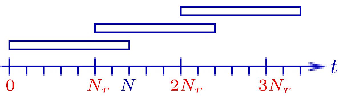
Figure 1. Receding horizon control strategy: At $t=0$, $N$ future control commands are computed but only first $N_{r}$ of them are applied; the process repeats after every $N_{r}$ time steps.

3. Output feedback policies

In this section we describe two important ingredients of SPC in the presence of incomplete state information. First of all, we need to estimate the states of the system given its output, and secondly, choose a suitable policy in terms of saturated innovations [11].

3.1. Estimator

For $t,s\in\mathds{N}$ $t\geqslant s$ let us define $\hat{x}_{t\mid s}\coloneqq\mathds{E}_{\mathfrak{Y}_{s}}\left[x_{t}\right]$ and

$$P_{t\mid s}\coloneqq\mathds{E}_{\mathfrak{Y}_{s}}\left[(x_{t}-\hat{x}_{t\mid s})(x_{t}-\hat{x}_{t\mid s})^{\top}\right].$$

For simplicity of notation we denote $\hat{x}_{t\mid t}$ by $\hat{x}_{t}$ and $P_{t\mid t}$ by $P_{t}$. We need a fundamental result related to Kalman filtering, which is stated in [9, p.102]. Let us define the estimation error vector $e_{t}\coloneqq x_{t}-\hat{x}_{t}$. Let

$$K_{t}\coloneqq(AP_{t}A^{\top}+\Sigma_{w})C^{\top}\Bigl{(}C(AP_{t}A^{\top}+\Sigma_{w})C^{\top}+\Sigma_{\varsigma}\Bigr{)}^{-1},$$

$$\Gamma_{t}\coloneqq I_{d}-K_{t}C,\text{ and }\phi_{t}\coloneqq\Gamma_{t}A.$$

The filter equations in [9, p.102] are used to find the evolution of the estimator error over one optimization horizon as follows:

(7) $$e_{t:N+1}=\mathcal{F}_{t}e_{t}+\mathcal{G}_{t}w_{t:N}-\mathcal{H}_{t}\varsigma_{t:N+1},$$

where $\mathcal{F}_{t}\coloneqq\begin{bmatrix}I_{d}\\ \phi_{t}\\ \phi_{t+1}\phi_{t}\\ \vdots\\ \phi_{t+N-1}\cdots\phi_{t}\end{bmatrix}$, $\mathcal{G}_{t}\coloneqq\begin{bmatrix}0&\cdots&0&0\\ \Gamma_{t}&\cdots&0&0\\ \phi_{t+1}\Gamma_{t}&\cdots&0&0\\ \vdots&\cdots&\vdots&\vdots\\ \phi_{t+N-2}\cdots\phi_{t+1}\Gamma_{t}&\cdots&\Gamma_{t+N-1}&0\\ \phi_{t+N-1}\cdots\phi_{t+1}\Gamma_{t}&\cdots&\phi_{t+N-1}\Gamma_{t+N-2}&\Gamma_{t+N-1}\end{bmatrix}$, $\mathcal{H}_{t}\coloneqq\begin{bmatrix}0&0&\cdots&0&0\\ 0&K_{t}&\cdots&0&0\\ 0&\phi_{t+1}K_{t}&\cdots&0&0\\ 0&\vdots&\cdots&\vdots&\vdots\\ 0&\phi_{t+N-2}\cdots\phi_{t+1}K_{t}&\cdots&K_{t+N-1}&0\\ 0&\phi_{t+N-1}\cdots\phi_{t+1}K_{t}&\cdots&\phi_{t+N-1}K_{t+N-2}&K_{t+N-1}\end{bmatrix}$. Since the optimization is done every $N_{r}$ time steps, we find $\hat{x}_{t+N_{r}}$ by using (1) and the filter equations [9, p.102] as:

(8) $$\hat{x}_{t+N_{r}}=A^{N_{r}}\hat{x}_{t}+\mathrm{R}_{N_{r}}(A,B)u_{t:N_{r}}+\Xi_{t+N_{r}-1},$$

where

$$\Xi_{t+N_{r}-1}=\begin{bmatrix}A^{N_{r}-1}K_{t}CA&\cdots&K_{t+N_{r}-1}CA\end{bmatrix}e_{t:N_{r}}$$

$$+\begin{bmatrix}A^{N_{r}-1}K_{t}C&A^{N_{r}-2}K_{t+1}C&\cdots&K_{t+N_{r}-1}C\end{bmatrix}w_{t:N_{r}}$$

$$+\begin{bmatrix}A^{N_{r}-1}K_{t}&A^{N_{r}-2}K_{t+1}&\cdots&K_{t+N_{r}-1}\end{bmatrix}\varsigma_{t+1:N_{r}}.$$

The quantity $\Xi_{t+N_{r}-1}$ in (8) is such that $\mathds{E}_{\mathfrak{Y}_{t}}\left[\Xi_{t+N_{r}-1}\right]=\mathbf{0}$ and it admits a bound:

Proposition 1.

([8, Proposition 3]) There exists some $T^{\prime},\beta>0$ such that $\mathds{E}_{\mathfrak{Y}_{t}}\left[\left\|\Xi_{t+N_{r}-1}\right\|\right]\leqslant\beta$ for all $t\geqslant T^{\prime}$.

3.2. Control policy class

We select the affine parametrization of control policies [17, 18, 19] under output feedback. It is demonstrated in [11] that, in the absence of control bounds, optimization over innovation feedback $(y_{t}-\hat{y}_{t})$ leads to convex problems. The innovation sequence for one optimization horizon is then given by:

(9) $$y_{t:N+1}-\hat{y}_{t:N+1}=\mathcal{C}\mathcal{F}_{t}e_{t}+\mathcal{C}\mathcal{G}_{t}w_{t:N}+(I-\mathcal{C}\mathcal{H}_{t})\varsigma_{t:N+1},$$

where $\hat{y}_{t:N+1}=\mathcal{C}\hat{x}_{t:N+1}$, $\mathcal{F}_{t},\mathcal{G}_{t}$ and $\mathcal{H}_{t}$ are as in (7), and $\mathcal{C}$ is defined in (4). However, this policy is inadmissible because controls are bounded. To satisfy hard bounds on the controls while retaining computational tractability, we consider affine parametrization in terms of the saturated values of innovation feedback: We periodically minimize the cost (3) over the following causal feedback policy for $\ell=0,\cdots,N-1$,

(10) $$u_{t+\ell}=\boldsymbol{\eta}_{t+\ell}+\sum_{i=0}^{\ell}\theta_{\ell,t+i}\mathfrak{\psi}_{i}(y_{t+i}-\hat{y}_{t+i}),$$

where $\mathfrak{\psi}_{i}:\mathds{R}^{q}\longrightarrow\ \mathds{R}^{q}$ is a measurable map for each $i$ such that $\left\|\mathfrak{\psi}_{i}(y_{t+i}-\hat{y}_{t+i})\right\|_{\infty}\leqslant\mathfrak{\psi}_{\max}$. The above control policy class (10) can be represented in a compact form as follows:

(11) $$u_{t:N}=\boldsymbol{\eta}_{t}+\boldsymbol{\Theta}_{t}\mathfrak{\psi}(y_{t:N+1}-\hat{y}_{t:N+1})$$

where $\boldsymbol{\eta}_{t}\in\mathds{R}^{mN}$ $\mathfrak{\psi}\coloneqq\begin{bmatrix}\mathfrak{\psi}_{0}^{\top}&\cdots&\mathfrak{\psi}_{N}^{\top}\end{bmatrix}$ and $\boldsymbol{\Theta}_{t}$ is the following block triangular matrix

$$\boldsymbol{\Theta}_{t}=\begin{bmatrix}\theta_{0,t}&\mathbf{0}&\cdots&\mathbf{0}&\mathbf{0}&\mathbf{0}\\ \theta_{1,t}&\theta_{1,t+1}&\cdots&\mathbf{0}&\mathbf{0}&\mathbf{0}\\ \vdots&\vdots&\vdots&\vdots&\vdots&\vdots\\ \theta_{N-1,t}&\theta_{N-1,t+1}&\cdots&\theta_{N-1,t+N-2}&\theta_{N-1,t+N-1}&\mathbf{0}\end{bmatrix},$$

with each $\theta_{k,\ell}\in\mathds{R}^{m\times q}$ and

$$\left\|\mathfrak{\psi}(y_{t:N+1}-\hat{y}_{t:N+1})\right\|_{\infty}\leqslant\mathfrak{\psi}_{\max}.$$

We choose $\mathfrak{\psi}_{i}$’s to be component-wise odd functions, e.g., standard saturation function, sigmoidal function, etc.

Figure 2. The Kalman filter employs the measurement $y_{t}$ to estimate the state $\hat{x}_{t}$ and is aware of the control $u_{t}$.

4. Stability

It is well known that the construction of a robust positively invariant set is not possible in the presence of Gaussian noise [2, §3.4]. Therefore, standard deterministic Lyapunov based arguments for proving stability are not applicable. Moreover, a linear stochastic system cannot be globally stabilized with the help of bounded controls [16, Theorem 1.7, Open problem 1.3] if the nominal plant has spectral radius larger than unity. Under this fundamental limitation, we restrict our attention to Lyapunov stable plants for ensuring stability. We establish the property of mean-square boundedness of the closed-loop plant under 3. This class of systems is indeed, till date, the largest class of linear time invariant systems that can be globally stabilized with bounded control actions. We recall the following definition:

Definition 1.

[13, §III.A] An $\mathds{R}^{d}$-valued random process $(x_{t})_{t\in\mathds{N}_{0}}$ with given initial measurement of output $\mathfrak{Y}_{0}$ is said to be mean-square bounded if

$$\sup_{t\in\mathds{N}}\mathds{E}_{\mathfrak{Y}_{0}}[\left\|x_{t}\right\|^{2}]<+\infty.$$

Note that a Lyapunov stable system matrix $A$ can be decomposed [20] into a Schur stable part $A_{s}$ and an orthogonal part $A_{o}$, resulting in recursion (8) as follows:

(12) $$\begin{bmatrix}\hat{x}_{t+1}^{o}\\ \hat{x}_{t+1}^{s}\end{bmatrix}=\begin{bmatrix}A_{o}\hat{x}_{t}^{o}\\ A_{s}\hat{x}_{t}^{s}\end{bmatrix}+\begin{bmatrix}B_{o}\\ B_{s}\end{bmatrix}u_{t}+\begin{bmatrix}\Xi_{t}^{o}\\ \Xi_{t}^{s}\end{bmatrix},$$

where ${\hat{x}}_{t}^{s}\in\mathds{R}^{d_{s}}$ , ${\hat{x}}_{t}^{o}\in\mathds{R}^{d_{o}}$, $d=d_{o}+d_{s}$, and $\Xi_{t}$ is defined in (8). Linear systems with Schur stable matrices are automatically stable (in suitable sense) under bounded controls, but stability of orthogonal systems in presence of stochastic noise is not obvious. The following stability constraint for orthogonal subsystem was presented in [8]:

(13) $$\begin{aligned} \left\|A_{o}^{\kappa}\hat{x}^{o}_{t}+\mathrm{R}_{\kappa}(A_{o},B_{o})u_{t:\kappa}\right\|&\leqslant\left\|\hat{x}^{o}_{t}\right\|-(\beta+\dfrac{\varepsilon^{\prime}}{2})\\ \text{ whenever }\left\|\hat{x}^{o}_{t}\right\|&\geqslant\beta+\varepsilon^{\prime},\end{aligned}$$

where $\varepsilon^{\prime}>0$, $\beta$ is as defined in Proposition 1, and $\kappa$ is the reachability index of the matrix pair $(A_{o},B_{o})$. Mean square boundedness of the closed-loop system with the above stability constraint was proved in [8] under large enough control authority. In particular, it was assumed in [8] that

$$u_{\max}\geqslant\sigma_{1}\left(\mathrm{R}_{N_{r}}(A_{o},B_{o})^{+}\right)(\beta+\dfrac{\varepsilon^{\prime}}{2}).$$

Let us consider the following example.

Example 1.

Let us consider the dynamics (12) when $A_{o}=1,d_{s}=0$:

(14) $$\begin{aligned} &\hat{x}_{t+1}^{o}=\hat{x}_{t}^{o}+u_{t}+\Xi_{t}^{o},\\ &\hat{y}^{o}_{t}=\hat{x}_{t}^{o},\quad y_{t}^{o}=x_{t}^{o}+\varsigma_{t}^{o}.\end{aligned}$$

Then the drift condition (13) given in [8] requires a scalar control such that $\left|\hat{x}_{t}^{o}+u_{t}\right|-\left|\hat{x}_{t}^{o}\right|\leqslant-(\beta+\dfrac{\varepsilon^{\prime}}{2})$ for all $\hat{x}_{t}^{o}$. Here equality holds when $u_{t}$ has magnitude $\beta+\dfrac{\varepsilon^{\prime}}{2}$ and sign opposite to that of $\hat{x}_{t}^{o}$. Since $\beta$ depends on the bound on the uncertainty (see Proposition 1), stability does not follow from [8, Theorem 1] when $u_{\max}<\beta+\dfrac{\varepsilon^{\prime}}{2}$. $\hfill\square$

However, this lower bound on the control authority is artificial and we show that it can be removed if different drift conditions are employed, resulting in different stability constraints. We have the following Lemma.

Lemma 1.

Consider the orthogonal part of the system (12). If there exists a $\kappa$-history dependent policy such that for any given $r>0,\text{ and }0<\zeta<\frac{u_{\max}}{\sqrt{d_{o}}\sigma_{1}\left(\mathrm{R}_{\kappa}(A_{o},B_{o})^{+}\right)},$ and for any $t=0,\kappa,2\kappa,...$, the control $u_{t:\kappa}\in\mathds{U}^{\kappa}$ is chosen such that for $j=1,2,\cdots,d_{o}$ the following conditions hold:

(15a) $$\mathds{E}_{\mathfrak{Y}_{t}}\left[\left((A_{o}^{\kappa})^{\top}\mathrm{R}_{\kappa}(A_{o},B_{o})u_{t:\kappa}\right)^{(j)}\right] \leqslant-\zeta\text{ if }\left(\hat{x}^{o}_{t}\right)^{(j)}>r,\text{ and}$$

(15b) $$\mathds{E}_{\mathfrak{Y}_{t}}\left[\left((A_{o}^{\kappa})^{\top}\mathrm{R}_{\kappa}(A_{o},B_{o})u_{t:\kappa}\right)^{(j)}\right] \geqslant\zeta\text{ if }\left((\hat{x}^{o}_{t}\right)^{(j)}<-r.$$

Successive application of this policy renders the orthogonal part of the closed-loop system (12) mean-square bounded; i.e. there exist $T,\gamma_{o}>0$ such that $\mathds{E}_{\mathfrak{Y}_{T}}\left[\left\|\hat{x}_{t}^{o}\right\|^{2}\right]\leqslant\gamma_{o}$ for all $t\geqslant T$.

A proof of Lemma 1 is given in the appendix.
In order to implement the drift conditions (15) with the help of a tractable optimization program, we consider the first $\kappa$ blocks of (11)

(16) $$u_{t:\kappa}=(\boldsymbol{\eta}_{t})_{1:\kappa m}+(\boldsymbol{\Theta}_{t})_{1:\kappa m}\mathfrak{\psi}(y_{t:N+1}-\hat{y}_{t:N+1})$$

and substitute them in (15). Let us separate the first $q$ columns of the gain matrix $\boldsymbol{\Theta}_{t}$ and the first $q$ rows of the saturated innovation sequence such that $\boldsymbol{\Theta}_{t}=\begin{bmatrix}\boldsymbol{\Theta}_{t}^{(:,t)}&\boldsymbol{\Theta}_{t}^{\prime}\end{bmatrix}$ and $\mathfrak{\psi}(y_{t:N+1}-\hat{y}_{t:N+1})=\begin{bmatrix}\mathfrak{\psi}_{0}(y_{t}-\hat{y}_{t})\\ \mathfrak{\psi}^{\prime}(y_{t+1:N}-\hat{y}_{t+1:N})\end{bmatrix}$, where $\boldsymbol{\Theta}_{t}^{(:,t)}$ represents the first $q$ columns of $\boldsymbol{\Theta}_{t}$, other notations are clear from the context. We get the following stability constraints for $\varepsilon>0$:

$$\quad\Biggl{(}(A_{o}^{\kappa})^{\top}\mathrm{R}_{\kappa}(A_{o},B_{o})\left((\boldsymbol{\eta}_{t})_{1:\kappa m}+(\boldsymbol{\Theta}_{t}^{(:,t)})_{1:\kappa m}\mathfrak{\psi}_{0}(y_{t}-\hat{y}_{t})\right)\Biggr{)}^{(j)}\leqslant-\zeta$$

(17a) $$\quad\quad\text{if }\left(\hat{x}^{o}_{t}\right)^{(j)}\geqslant r+\varepsilon,\text{ and }$$

$$\quad\Biggl{(}(A_{o}^{\kappa})^{\top}\mathrm{R}_{\kappa}(A_{o},B_{o})\left((\boldsymbol{\eta}_{t})_{1:\kappa m}+(\boldsymbol{\Theta}_{t}^{(:,t)})_{1:\kappa m}\mathfrak{\psi}_{0}(y_{t}-\hat{y}_{t})\right)\Biggr{)}^{(j)}\geqslant\zeta$$

(17b) $$\quad\quad\text{if }\left(\hat{x}^{o}_{t}\right)^{(j)}\leqslant-r-\varepsilon,$$

where $r,\zeta$ and $j$ are as in (15).

Example 2.

Let us consider the dynamics (14). The conditions (17) provide expected drift towards the interval $]-r-\varepsilon,r+\varepsilon[$ in one step whenever $\hat{x}_{t}^{o}$ is outside that interval. The amount of constant negative drift $\zeta$ can be selected from the interval $]0,u_{\max}[$ to respect the hard bound on control. $\hfill\square$

5. Main results

In this section we recast the constrained optimal control problem (6) as a convex quadratic optimization program that is recursively feasible, and its receding horizon implementation ensures mean-square boundedness of the system states. We can select the recalculation interval $N_{r}$ such that $\kappa\leqslant N_{r}\leqslant N$. For simplicity, we choose $N_{r}=\kappa\leqslant N$. Let us define $\Pi_{y_{t}}=\mathfrak{\psi}_{0}(y_{t}-\hat{y}_{t})\mathfrak{\psi}_{0}(y_{t}-\hat{y}_{t})^{\top}$, $\Sigma_{\mathfrak{\psi}}=\mathds{E}\Bigl{[}\mathfrak{\psi}^{\prime}(y_{t+1:N}-\hat{y}_{t+1:N})\mathfrak{\psi}^{\prime}(y_{t+1:N}-\hat{y}_{t+1:N})^{\top}\Bigr{]}$, $\Sigma_{\mathfrak{\psi}^{\prime}w}=\mathds{E}\Biggl{[}\mathfrak{\psi}^{\prime}(y_{t+1:N}-\hat{y}_{t+1:N})w_{t:N}^{\top}\Biggr{]}$, $\Sigma_{e\mathfrak{\psi}^{\prime}}=\mathds{E}\Bigl{[}\mathfrak{\psi}^{\prime}(y_{t+1:N}-\hat{y}_{t+1:N})e_{t}^{\top}\Bigr{]}$ and $\alpha\coloneqq\mathcal{B}^{\top}\mathcal{Q}\mathcal{B}+\mathcal{R}$. We have the following theorems:

Theorem 1.

For every time $t=0,N_{r},2N_{r},\cdots$, the optimal control problem (6) can be written as the following convex quadratic, (globally) feasible program:

$$\operatorname*{min}_{\boldsymbol{\eta}_{t},\boldsymbol{\Theta}_{t}} \quad\boldsymbol{\eta}_{t}^{\top}\alpha\boldsymbol{\eta}_{t}+\operatorname{tr}(\alpha\boldsymbol{\Theta}_{t}^{(:,t)}\Pi_{y_{t}}(\boldsymbol{\Theta}_{t}^{(:,t)})^{\top})+\operatorname{tr}(\alpha\boldsymbol{\Theta}_{t}^{\prime}\Sigma_{\mathfrak{\psi}}(\boldsymbol{\Theta}_{t}^{\prime})^{\top})+2\hat{x}_{t}^{\top}\mathcal{A}^{\top}\mathcal{Q}\mathcal{B}\boldsymbol{\eta}_{t}$$

(18) $$+2(\boldsymbol{\eta}_{t}^{\top}\alpha+\hat{x}_{t}^{\top}\mathcal{A}^{\top}\mathcal{Q}\mathcal{B})\boldsymbol{\Theta}_{t}^{(:,t)}\mathfrak{\psi}_{0}(y_{t}-\hat{y}_{t})+2\operatorname{tr}\Bigl{(}\mathcal{D}^{\top}\mathcal{Q}\mathcal{B}\boldsymbol{\Theta}_{t}^{\prime}\Sigma_{\mathfrak{\psi}^{\prime}w}+\mathcal{A}^{\top}\mathcal{Q}\mathcal{B}\boldsymbol{\Theta}_{t}^{\prime}\Sigma_{e\mathfrak{\psi}^{\prime}}\Bigr{)}.$$

(19) $$\operatorname*{s.\ t.} \quad\left|\boldsymbol{\eta}_{t}^{(i)}\right|+\left\|\boldsymbol{\Theta}_{t}^{(i,:)}\right\|_{1}\mathfrak{\psi}_{\max}\leqslant u_{\max}\;\forall i=1,\cdots,Nm,$$

(20) $$\quad\text{stability constraints }\eqref{e:stability constraint}.$$

The matrices $\Sigma_{\mathfrak{\psi}w}$, $\Sigma_{\mathfrak{\psi}}$ and $\Sigma_{e\mathfrak{\psi}}$ required in the above optimization program depend on $y_{t:N+1}-\hat{y}_{t:N+1}$, which depend on the time variant quantity $P_{t}$. Since $P_{t}$ converges asymptotically to a stationary value [8, §4.4], $\Sigma_{\mathfrak{\psi}w}$, $\Sigma_{\mathfrak{\psi}}$ and $\Sigma_{e\mathfrak{\psi}}$ can be easily computed offline empirically via classical Monte Carlo methods [21]. Computations for determining our policy were carried out in the MATLAB-based software package YALMIP [22], and were solved using SDPT3-4.0 [23].

Theorem 2.

The successive applications of the controls given by the optimization program in Theorem 1 above renders the closed-loop system mean-square bounded for any positive bound on control.

Proofs of Theorem 1 and Theorem 2 are provided in the appendix.

6. Numerical Experiment

We present numerical experiments to illustrate our results and compare our approach against [8] with same objectiive function but different stability constraints. Let us consider the four dimensional linear stochastic system (1) with matrices lifted from [8]:

$$A=\begin{bmatrix}0.9&0&0&0\\ 0&1&0&0\\ 0&0&0&-1\\ 0&0&1&0\end{bmatrix},B=\begin{bmatrix}0\\ 1\\ 0\\ 1\end{bmatrix},C=I_{4}.$$

The simulation data was chosen to be $x_{0}\sim N(0,I_{4})$, $w_{t}\sim N(0,I_{4})$, $\varsigma_{t}\sim N(0,I_{4})$.

We solved a constrained finite-horizon optimal control problem corresponding to states and control weights $Q=I_{4},Q_{f}=I_{4},R=1$. We selected an optimization horizon, $N=5$, recalculation interval $N_{r}=\kappa=3$ and simulated the system responses. We selected the nonlinear bounded term $\mathfrak{\psi}(\cdot)$ in our policy to be a vector of scalar sigmoidal functions

$$\varphi(\xi)=\frac{1-e^{-\xi}}{1+e^{-\xi}}$$

applied to each coordinate of innovation sequence. We plot empirical mean square bound with respect to $u_{\max}$ picked from the set $\{0.1,0.5,1,2,3,4,5,10,20\}$. All the averages are taken over 100 sample paths for 90 time steps. The optimization program of [8] becomes infeasible when $u_{\max}\leqslant 3$, because the stability constraints used in [8] require a larger bound on the controls. Therefore, we modified the optimization algorithm of [8]. For our purposes we have forced the control values to $\mathbf{0}$ whenever the termination code of the solver is not equal to $0$. Our proposed controller performs better than this modified controller for $u_{\max}=0.1,0.5,1,2$, and yields similar performance for $u_{\max}=3$. For $u_{\max}\geqslant 4$, all three controllers perform similarly in terms of the mean square bound of the closed-loop states.

Figure 3. Empirical mean square bounds against $u_{\max}$.

7. Epilogue

We presented a tractable method for predictive control of linear stochastic control systems in the presence of incomplete and corrupt state information. We proved that given any fixed control bound, our receding horizon strategy yields a closed-loop system with mean-square bounded states whenever the system matrix $A$ is Lyapunov stable. Our results are valid when the process and measurement uncertainties are independent and Gaussian. In future work, we aim to incorporate control channel noise into our framework.

Appendix

Lemma 2.

[8, Lemma 8] Consider the system (1) and assume that $P_{0}\succeq 0$. Then, there exists a time $T^{\prime}\in\mathds{N}$ and constant $\rho>0$ such that $\mathds{E}_{\mathfrak{Y}_{t}}\left[\left\|x_{t}-\hat{x}_{t}\right\|^{2}\right]=\operatorname{tr}(P_{t})\leqslant\rho$ for all $t\geqslant T^{\prime}$.

Theorem 3 ([24, Theorem 1, Corollary 2]).

Let $(X_{t})_{t\in\mathds{N}}$ be a family of real valued random variables on a probability space $(\Omega,\mathfrak{F},\mathds{P})$, adapted to a filtration $(\mathfrak{F}_{t})_{t\in\mathds{N}}$. Suppose that there exist scalars $J,M,a>0$ such that

(21) $$\mathds{E}_{\mathfrak{F}_{t}}[X_{t+1}-X_{t}]\leqslant-a\quad\text{on the event }X_{t}>J,\text{ and}$$

(22) $$\mathds{E}\bigl{[}\left|X_{t+1}-X_{t}\right|^{4}\,\big{|}\,X_{0},\ldots,X_{t}\bigr{]}\leqslant M\quad\text{for all }t\in\mathds{N}.$$

Then there exists a constant $C>0$ such that $\sup_{t\in\mathds{N}}\mathds{E}\bigl{[}((X_{t})_{+})^{2}\mid\mathfrak{F}_{0}\bigr{]}\leqslant C$.

Proof of Lemma 1.

Let us consider the $\kappa$-sub-sampled process of orthogonal subsystem of (12) by using (8): $\hat{x}_{\kappa(t+1)}^{o}=A_{o}^{\kappa}\hat{x}_{\kappa t}^{o}+\mathrm{R}_{\kappa}(A_{o},B_{o})u_{\kappa t:\kappa}+\Xi_{\kappa t+\kappa-1}^{o}.$ Define $z_{\kappa t}\coloneqq(A_{o}^{\top})^{\kappa t}\hat{x}_{\kappa t}^{o}$. It follows that

(23) $$z_{\kappa(t+1)} =z_{\kappa t}+(A_{o}^{\top})^{\kappa(t+1)}\mathrm{R}_{\kappa}(A_{o},B_{o})u_{\kappa t:\kappa}+(A_{o}^{\top})^{\kappa(t+1)}\Xi_{\kappa t+\kappa-1}^{o}$$

$$=z_{\kappa t}+\tilde{u}_{\kappa t}+\tilde{\Xi}_{\kappa t},$$

where, $\tilde{u}_{\kappa t}=(A_{o}^{\top})^{\kappa(t+1)}\mathrm{R}_{\kappa}(A_{o},B_{o})u_{\kappa t:\kappa},\tilde{\Xi}_{\kappa t}=(A_{o}^{\top})^{\kappa(t+1)}\Xi_{\kappa t+\kappa-1}^{o}.$ Let $\mathfrak{F}_{\kappa t}$ denote the $\sigma$-algebra generated by $\{\mathfrak{Y}_{\kappa\ell}\,|\,\ell=0,1,\ldots,t\}$. Now, we have

$$\mathds{E}_{\mathfrak{F}_{\kappa t}}\bigl{[}z_{\kappa(t+1)}-z_{\kappa t}\bigr{]}=\mathds{E}_{\mathfrak{F}_{\kappa t}}[\tilde{u}_{\kappa t}+\tilde{\Xi}_{\kappa t}]=\mathds{E}_{\mathfrak{F}_{\kappa t}}[\tilde{u}_{\kappa t}]$$

Let us consider the control sequence

(24) $$u_{\kappa t:\kappa}=-\mathrm{R}_{\kappa}(A_{o},B_{o})^{+}A_{o}^{\kappa(t+1)}\operatorname{sat}_{r,\zeta}^{\infty}\bigl{(}(A_{o}^{\top})^{\kappa t}\hat{x}^{o}_{\kappa t}\bigr{)}.$$

It can be easily verified that $u_{\kappa t+\ell}\in\mathds{U}$ for $\ell=0,\ldots,\kappa-1$ whenever $0<\zeta<\frac{u_{\max}}{\sqrt{d_{o}}\sigma_{1}\left(\mathrm{R}_{\kappa}(A_{o},B_{o})^{+}\right)}$. For the $j$-th component $z^{(j)}_{\kappa t}$ of $z_{\kappa t}$ we see that

$$\mathds{E}_{\mathfrak{F}_{\kappa t}}\bigl{[}z^{(j)}_{\kappa(t+1)}-z^{(j)}_{\kappa t}\bigr{]} =\mathds{E}_{\mathfrak{F}_{\kappa t}}\bigl{[}\tilde{u}_{\kappa t}^{(j)}\bigr{]}$$

$$=\left((A_{o}^{\top})^{\kappa t}\mathds{E}\left[(A_{o}^{\top})^{\kappa}\mathrm{R}_{\kappa}(A_{o},B_{o})u_{\kappa t:\kappa}\right]\right)^{(j)}=-\zeta,$$

whenever $z^{(j)}_{\kappa t}=\left((A_{o}^{\top})^{\kappa t}\hat{x}_{\kappa t}^{o}\right)^{(j)}>r$, and similarly

$$\mathds{E}_{\mathfrak{F}_{\kappa t}}\bigl{[}z^{(j)}_{\kappa(t+1)}-z^{(j)}_{\kappa t}\bigr{]}=\zeta\quad\text{whenever }z^{(j)}_{\kappa t}<-r.$$

If we define $X_{t}\coloneqq z_{\kappa t}^{(j)},J\coloneqq r,a\coloneqq\zeta$, we can observe that the the first condition of Theorem 3 is satisfied for a given control sequence (24). For an arbitrary control sequence $u_{\kappa t:\kappa}$ the first condition of Theorem 3 is satisfied if (15a) is satisfied. Similarly, for $-X_{t}\coloneqq z_{\kappa t}^{(j)}$ the first condition of Theorem 3 is satisfied if (15b) is satisfied. The rest of the proof follows as in the proof of [16, Theorem 1.2]. We include the salient steps for completeness. A straightforward computation relying on uniform boundedness of the control and the moment boundedness of $\Xi_{\kappa t+\kappa-1}$ (see Proposition 1) shows that there exists an $M>0$ such that

$$\mathds{E}\Bigl{[}\left|z^{(j)}_{\kappa(t+1)}-z^{(j)}_{\kappa t}\right|^{4}\,\Big{|}\,z^{(j)}_{\kappa t},\ldots,z^{(j)}_{0}\Bigr{]}$$

$$=\mathds{E}\Bigl{[}\left|\tilde{u}_{\kappa t}^{(j)}+(\tilde{\Xi}_{\kappa t})^{(j)}\right|^{4}\,\Big{|}\,z^{(j)}_{\kappa t},\ldots,z^{(j)}_{0}\Bigr{]}\leqslant M\quad\text{for all }t\geqslant\frac{T}{\kappa},$$

where $T\coloneqq\kappa\left\lceil\frac{T^{\prime}}{\kappa}\right\rceil\geqslant T^{\prime}$ and $T^{\prime}$ is defined in Proposition 1. Now [24, Theorem 1] guarantees the existence of constants $C^{(j)}_{1},C^{(j)}_{2}>0$, $j=1,\ldots,d_{o}$, such that

$$\mathds{E}_{\mathfrak{Y}_{T}}\Bigl{[}\left(\bigl{(}z^{(j)}_{\kappa t}\bigr{)}_{+}\right)^{2}\Bigr{]}\leqslant C^{(j)}_{1}\quad\text{and}\quad\mathds{E}_{\mathfrak{Y}_{T}}\Bigl{[}\left(\bigl{(}z^{(j)}_{\kappa t}\bigr{)}_{-}\right)^{2}\Bigr{]}\leqslant C^{(j)}_{2}\text{ for all }t\geqslant\frac{T}{\kappa}.$$

Since $\left|\delta\right|=\delta_{+}+\delta_{-}=\delta_{+}+(-\delta)_{+}$ for any $\delta\in\mathds{R}$, and for any $\delta\in\mathds{R}^{d_{o}}$, $\left\|\delta\right\|^{2}=\sum_{j=1}^{d_{o}}\left|\delta^{(j)}\right|^{2}\leqslant 2\sum_{j=1}^{d_{o}}\bigl{(}(\delta^{(j)}_{+})^{2}+(\delta^{(j)}_{-})^{2}\bigr{)},$ we see at once that the preceding bounds imply

$$\mathds{E}_{\mathfrak{Y}_{T}}\bigl{[}\left\|z_{\kappa t}\right\|^{2}\bigr{]}<C\quad\text{for some constant $C>0$}\text{ for all }t\geqslant\frac{T}{\kappa}.$$

Since $\hat{x}_{\kappa t}^{o}$ is derived from $z_{\kappa t}$ by an orthogonal transformation, it immediately follows that $\mathds{E}_{\mathfrak{Y}_{T}}\bigl{[}\left\|\hat{x}^{o}_{\kappa t}\right\|^{2}\bigr{]}\leqslant C$ for all $t\geqslant\frac{T}{\kappa}$. A standard argument (e.g., as in [16]) now suffices to conclude from mean-square boundedness of the $\kappa$-subsampled process $(\hat{x}^{o}_{\kappa t})_{t\in\mathds{N}}$ the same property of the original process $(\hat{x}^{o}_{t})_{t\in\mathds{N}}$. In particular, there exists $\gamma_{o}$ such that

$$\mathds{E}_{\mathfrak{Y}_{T}}\left[\left\|\hat{x}^{o}_{t}\right\|^{2}\right]\leqslant\gamma_{o}\text{ for all }t\geqslant T.$$

∎

Proof of Theorem 1.

Consider the objective function (3). We substitute the stacked state vector (4a) in the objective function.

$$V_{t}=\mathds{E}_{\mathfrak{Y}_{t}}\left[\sum_{k=0}^{N-1}(\left\|x_{t+k}\right\|^{2}_{Q_{k}}+\left\|u_{t+k}\right\|^{2}_{R_{k}})+\left\|x_{t+N}\right\|^{2}_{Q_{N}}\right]$$

$$=\mathds{E}_{\mathfrak{Y}_{t}}\left[\left\|\mathcal{A}x_{t}+\mathcal{B}u_{t:N}+\mathcal{D}w_{t:N}\right\|^{2}_{\mathcal{Q}}+\left\|u_{t:N}\right\|^{2}_{\mathcal{R}}\right]$$

$$=\mathds{E}_{\mathfrak{Y}_{t}}\Bigl{[}\left\|\mathcal{A}x_{t}\right\|^{2}_{\mathcal{Q}}+\left\|\mathcal{D}w_{t:N}\right\|^{2}_{\mathcal{Q}}+\left\|u_{t:N}\right\|^{2}_{\alpha}+2(x_{t}^{\top}\mathcal{A}^{\top}\mathcal{Q}\mathcal{B}+w_{t:N}^{\top}\mathcal{D}^{\top}\mathcal{Q}\mathcal{B})u_{t:N}$$

$$\quad+2x_{t}^{\top}\mathcal{A}^{\top}\mathcal{Q}\mathcal{D}w_{t:N}\Bigr{]},\text{ where }\alpha=\mathcal{B}^{\top}\mathcal{Q}\mathcal{B}+\mathcal{R}.$$

Let $\beta_{t}\coloneqq\mathds{E}_{\mathfrak{Y}_{t}}\left[\left\|\mathcal{A}x_{t}\right\|^{2}_{\mathcal{Q}}+\left\|\mathcal{D}w_{t:N}\right\|^{2}_{\mathcal{Q}}+2x_{t}^{\top}\mathcal{A}^{\top}\mathcal{Q}\mathcal{D}w_{t:N}\right]=\mathds{E}_{\mathfrak{Y}_{t}}\left[\left\|\mathcal{A}x_{t}\right\|^{2}_{\mathcal{Q}}+\left\|\mathcal{D}w_{t:N}\right\|^{2}_{\mathcal{Q}}\right]$, then

(25) $$V_{t}=\mathds{E}_{\mathfrak{Y}_{t}}\Bigl{[}\left\|u_{t:N}\right\|^{2}_{\alpha}+2(x_{t}^{\top}\mathcal{A}^{\top}\mathcal{Q}\mathcal{B}+w_{t:N}^{\top}\mathcal{D}^{\top}\mathcal{Q}\mathcal{B})u_{t:N}\Bigr{]}+\beta_{t}.$$

We substitute the stacked control vector (11) in (25) and for simplicity represent $\Delta_{y_{t}}=y_{t:N+1}-\hat{y}_{t:N+1}$ to get the following expression:

$$V_{t}=\mathds{E}_{\mathfrak{Y}_{t}}\Bigl{[}\left\|\boldsymbol{\eta}_{t}+\boldsymbol{\Theta}_{t}\mathfrak{\psi}(\Delta_{y_{t}})\right\|^{2}_{\alpha}+2(x_{t}^{\top}\mathcal{A}^{\top}\mathcal{Q}\mathcal{B}+w_{t:N}^{\top}\mathcal{D}^{\top}\mathcal{Q}\mathcal{B})\bigl{(}\boldsymbol{\eta}_{t}+\boldsymbol{\Theta}_{t}\mathfrak{\psi}(\Delta_{y_{t}})\bigr{)}\Bigr{]}+\beta_{t}$$

$$=\boldsymbol{\eta}_{t}^{\top}\alpha\boldsymbol{\eta}_{t}+\mathds{E}_{\mathfrak{Y}_{t}}\Bigl{[}\left\|\boldsymbol{\Theta}_{t}\mathfrak{\psi}(\Delta_{y_{t}})\right\|^{2}_{\alpha}+2\boldsymbol{\eta}_{t}^{\top}\alpha\boldsymbol{\Theta}_{t}\mathfrak{\psi}(\Delta_{y_{t}})+2(x_{t}^{\top}\mathcal{A}^{\top}\mathcal{Q}\mathcal{B}+w_{t:N}^{\top}\mathcal{D}^{\top}\mathcal{Q}\mathcal{B})\boldsymbol{\Theta}_{t}\mathfrak{\psi}(\Delta_{y_{t}})\Bigr{]}$$

$$+\mathds{E}_{\mathfrak{Y}_{t}}\Bigl{[}2(x_{t}^{\top}\mathcal{A}^{\top}\mathcal{Q}\mathcal{B}+w_{t:N}^{\top}\mathcal{D}^{\top}\mathcal{Q}\mathcal{B})\boldsymbol{\eta}_{t}\Bigr{]}+\beta_{t}$$

$$=\boldsymbol{\eta}_{t}^{\top}\alpha\boldsymbol{\eta}_{t}+\mathds{E}_{\mathfrak{Y}_{t}}\Bigl{[}\left\|\boldsymbol{\Theta}_{t}\mathfrak{\psi}(\Delta_{y_{t}})\right\|^{2}_{\alpha}+2\boldsymbol{\eta}_{t}^{\top}\alpha\boldsymbol{\Theta}_{t}\mathfrak{\psi}(\Delta_{y_{t}})+2(x_{t}^{\top}\mathcal{A}^{\top}\mathcal{Q}\mathcal{B}+w_{t:N}^{\top}\mathcal{D}^{\top}\mathcal{Q}\mathcal{B})\boldsymbol{\Theta}_{t}\mathfrak{\psi}(\Delta_{y_{t}})\Bigr{]}$$

$$\quad+2\mathds{E}_{\mathfrak{Y}_{t}}\Bigl{[}x_{t}^{\top}\mathcal{A}^{\top}\mathcal{Q}\mathcal{B}\boldsymbol{\eta}_{t}\Bigr{]}+\beta_{t}.$$

Since $\mathds{E}_{\mathfrak{Y}_{t}}\left[x_{t}\right]=\hat{x}_{t}$, we get the following expression:

(26) $$V_{t}=\boldsymbol{\eta}_{t}^{\top}\alpha\boldsymbol{\eta}_{t}+\mathds{E}_{\mathfrak{Y}_{t}}\Bigl{[}\left\|\boldsymbol{\Theta}_{t}\mathfrak{\psi}(\Delta_{y_{t}})\right\|^{2}_{\alpha}+2(\boldsymbol{\eta}_{t}^{\top}\alpha+x_{t}^{\top}\mathcal{A}^{\top}\mathcal{Q}\mathcal{B}+w_{t:N}^{\top}\mathcal{D}^{\top}\mathcal{Q}\mathcal{B})\boldsymbol{\Theta}_{t}\mathfrak{\psi}(\Delta_{y_{t}})\Bigr{]}$$

$$\quad+2\hat{x}_{t}^{\top}\mathcal{A}^{\top}\mathcal{Q}\mathcal{B}\boldsymbol{\eta}_{t}+\beta_{t}.$$

Let us consider the term $\mathds{E}_{\mathfrak{Y}_{t}}\left[\boldsymbol{\eta}_{t}^{\top}\alpha\boldsymbol{\Theta}_{t}\mathfrak{\psi}(\Delta_{y_{t}})\right]$. By observing $\mathds{E}_{\mathfrak{Y}_{t}}\left[\mathfrak{\psi}_{i}(y_{t+i}-\hat{y}_{t+i})\right]=\mathbf{0}$ for each $i=1,\ldots,N+1$, we get

$$\mathds{E}_{\mathfrak{Y}_{t}}\left[\boldsymbol{\eta}_{t}^{\top}\alpha\boldsymbol{\Theta}_{t}\mathfrak{\psi}(\Delta_{y_{t}})\right] =\boldsymbol{\eta}_{t}^{\top}\alpha\begin{bmatrix}\theta_{0,t}\\ \theta_{1,t}\\ \vdots\\ \theta_{N-1,t}\end{bmatrix}\mathfrak{\psi}_{0}(y_{t}-\hat{y}_{t})$$

(27) $$=\boldsymbol{\eta}_{t}^{\top}\alpha\boldsymbol{\Theta}_{t}^{(:,t)}\mathfrak{\psi}_{0}(y_{t}-\hat{y}_{t}),$$

where $\boldsymbol{\Theta}_{t}^{(:,t)}\coloneqq\begin{bmatrix}\theta_{0,t}\\ \theta_{1,t}\\ \vdots\\ \theta_{N-1,t}\end{bmatrix}$ represents the first $q$ columns of the gain matrix $\boldsymbol{\Theta}_{t}$. Let us consider the term $\mathds{E}_{\mathfrak{Y}_{t}}\Bigl{[}\left\|\boldsymbol{\Theta}_{t}\mathfrak{\psi}(\Delta_{y_{t}})\right\|^{2}_{\alpha}\Bigr{]}$. In order to make the offline computation easy we do the following manipulation:

$$\mathds{E}_{\mathfrak{Y}_{t}}\Bigl{[}\left\|\boldsymbol{\Theta}_{t}\mathfrak{\psi}(\Delta_{y_{t}})\right\|^{2}_{\alpha}\Bigr{]}$$

$$=\mathds{E}_{\mathfrak{Y}_{t}}\Biggl{[}\left\|\begin{bmatrix}\boldsymbol{\Theta}_{t}^{(:,t)}&\boldsymbol{\Theta}_{t}^{\prime}\end{bmatrix}\begin{bmatrix}\mathfrak{\psi}_{0}(y_{t}-\hat{y}_{t})\\ \mathfrak{\psi}^{\prime}(y_{t+1:N}-\hat{y}_{t+1:N})\end{bmatrix}\right\|^{2}_{\alpha}\Biggr{]}$$

$$=\mathds{E}_{\mathfrak{Y}_{t}}\Biggl{[}\begin{bmatrix}\mathfrak{\psi}_{0}(y_{t}-\hat{y}_{t})\\ \mathfrak{\psi}^{\prime}(y_{t+1:N}-\hat{y}_{t+1:N})\end{bmatrix}^{\top}\begin{bmatrix}\boldsymbol{\Theta}_{t}^{(:,t)}&\boldsymbol{\Theta}_{t}^{\prime}\end{bmatrix}^{\top}{\alpha}\begin{bmatrix}\boldsymbol{\Theta}_{t}^{(:,t)}&\boldsymbol{\Theta}_{t}^{\prime}\end{bmatrix}\begin{bmatrix}\mathfrak{\psi}_{0}(y_{t}-\hat{y}_{t})\\ \mathfrak{\psi}^{\prime}(y_{t+1:N}-\hat{y}_{t+1:N})\end{bmatrix}\Biggr{]}$$

$$=\operatorname{tr}\Biggl{(}\alpha\boldsymbol{\Theta}_{t}^{(:,t)}\mathfrak{\psi}_{0}(y_{t}-\hat{y}_{t})\mathfrak{\psi}_{0}(y_{t}-\hat{y}_{t})^{\top}(\boldsymbol{\Theta}_{t}^{(:,t)})^{\top}$$

$$\quad+\alpha\boldsymbol{\Theta}_{t}^{\prime}\mathds{E}_{\mathfrak{Y}_{t}}\Bigl{[}\mathfrak{\psi}^{\prime}(y_{t+1:N}-\hat{y}_{t+1:N})\mathfrak{\psi}^{\prime}(y_{t+1:N}-\hat{y}_{t+1:N})^{\top}(\boldsymbol{\Theta}_{t}^{\prime})^{\top}\Bigr{]}\Biggr{)}$$

(28) $$=\operatorname{tr}(\alpha\boldsymbol{\Theta}_{t}^{(:,t)}\Pi_{y_{t}}(\boldsymbol{\Theta}_{t}^{(:,t)})^{\top})+\operatorname{tr}(\alpha\boldsymbol{\Theta}_{t}^{\prime}\Sigma_{\mathfrak{\psi}}(\boldsymbol{\Theta}_{t}^{\prime})^{\top}),$$

where $\Pi_{y_{t}}=\mathfrak{\psi}_{0}(y_{t}-\hat{y}_{t})\mathfrak{\psi}_{0}(y_{t}-\hat{y}_{t})^{\top}$ and $\Sigma_{\mathfrak{\psi}}=\mathds{E}\Bigl{[}\mathfrak{\psi}^{\prime}(y_{t+1:N}-\hat{y}_{t+1:N})\mathfrak{\psi}^{\prime}(y_{t+1:N}-\hat{y}_{t+1:N})^{\top}\Bigr{]}$. Further, we simplify the term $\mathds{E}_{\mathfrak{Y}_{t}}\Bigl{[}w_{t:N}^{\top}\mathcal{D}^{\top}\mathcal{Q}\mathcal{B}\boldsymbol{\Theta}_{t}\mathfrak{\psi}(\Delta_{y_{t}})\Bigr{]}$ as follows:

$$\mathds{E}_{\mathfrak{Y}_{t}}\Bigl{[}w_{t:N}^{\top}\mathcal{D}^{\top}\mathcal{Q}\mathcal{B}\boldsymbol{\Theta}_{t}\mathfrak{\psi}(\Delta_{y_{t}})\Bigr{]}$$

$$=\mathds{E}_{\mathfrak{Y}_{t}}\Biggl{[}w_{t:N}^{\top}\mathcal{D}^{\top}\mathcal{Q}\mathcal{B}\begin{bmatrix}\boldsymbol{\Theta}_{t}^{(:,t)}&\boldsymbol{\Theta}_{t}^{\prime}\end{bmatrix}\begin{bmatrix}\mathfrak{\psi}_{0}(y_{t}-\hat{y}_{t})\\ \mathfrak{\psi}^{\prime}(y_{t+1:N}-\hat{y}_{t+1:N})\end{bmatrix}\Biggr{]}$$

$$=\operatorname{tr}\left(\mathcal{D}^{\top}\mathcal{Q}\mathcal{B}\boldsymbol{\Theta}_{t}^{\prime}\mathds{E}_{\mathfrak{Y}_{t}}\Biggl{[}\mathfrak{\psi}^{\prime}(y_{t+1:N}-\hat{y}_{t+1:N})w_{t:N}^{\top}\Biggr{]}\right)$$

(29) $$=\operatorname{tr}\left(\mathcal{D}^{\top}\mathcal{Q}\mathcal{B}\boldsymbol{\Theta}_{t}^{\prime}\Sigma_{\mathfrak{\psi}^{\prime}w}\right),$$

where $\Sigma_{\mathfrak{\psi}^{\prime}w}=\mathds{E}\Biggl{[}\mathfrak{\psi}^{\prime}(y_{t+1:N}-\hat{y}_{t+1:N})w_{t:N}^{\top}\Biggr{]}$. We simplify the term $\mathds{E}_{\mathfrak{Y}_{t}}\Bigl{[}x_{t}^{\top}\mathcal{A}^{\top}\mathcal{Q}\mathcal{B}\boldsymbol{\Theta}_{t}\mathfrak{\psi}(\Delta_{y_{t}})\Bigr{]}$ as follows:

$$\mathds{E}_{\mathfrak{Y}_{t}}\Bigl{[}x_{t}^{\top}\mathcal{A}^{\top}\mathcal{Q}\mathcal{B}\boldsymbol{\Theta}_{t}\mathfrak{\psi}(\Delta_{y_{t}})\Bigr{]}$$

$$=\mathds{E}_{\mathfrak{Y}_{t}}\Bigl{[}(x_{t}-\hat{x}_{t})^{\top}\mathcal{A}^{\top}\mathcal{Q}\mathcal{B}\boldsymbol{\Theta}_{t}\mathfrak{\psi}(\Delta_{y_{t}})\Bigr{]}+\mathds{E}_{\mathfrak{Y}_{t}}\Bigl{[}\hat{x}_{t}^{\top}\mathcal{A}^{\top}\mathcal{Q}\mathcal{B}\boldsymbol{\Theta}_{t}\mathfrak{\psi}(\Delta_{y_{t}})\Bigr{]}$$

$$=\mathds{E}_{\mathfrak{Y}_{t}}\Bigl{[}e_{t}^{\top}\mathcal{A}^{\top}\mathcal{Q}\mathcal{B}\boldsymbol{\Theta}_{t}\mathfrak{\psi}(\Delta_{y_{t}})\Bigr{]}+\hat{x}_{t}^{\top}\mathds{E}_{\mathfrak{Y}_{t}}\Bigl{[}\mathcal{A}^{\top}\mathcal{Q}\mathcal{B}\boldsymbol{\Theta}_{t}\mathfrak{\psi}(\Delta_{y_{t}})\Bigr{]}$$

$$=\mathds{E}_{\mathfrak{Y}_{t}}\Bigl{[}e_{t}^{\top}\mathcal{A}^{\top}\mathcal{Q}\mathcal{B}\boldsymbol{\Theta}_{t}\mathfrak{\psi}(\Delta_{y_{t}})\Bigr{]}+\hat{x}_{t}^{\top}\mathcal{A}^{\top}\mathcal{Q}\mathcal{B}\boldsymbol{\Theta}_{t}^{(:,t)}\mathfrak{\psi}_{0}(y_{t}-\hat{y}_{t})$$

$$=\operatorname{tr}\Bigl{(}\mathcal{A}^{\top}\mathcal{Q}\mathcal{B}\boldsymbol{\Theta}_{t}^{\prime}\mathds{E}_{\mathfrak{Y}_{t}}\Bigl{[}\mathfrak{\psi}^{\prime}(y_{t+1:N}-\hat{y}_{t+1:N})e_{t}^{\top}\Bigr{]}\Bigr{)}+\hat{x}_{t}^{\top}\mathcal{A}^{\top}\mathcal{Q}\mathcal{B}\boldsymbol{\Theta}_{t}^{(:,t)}\mathfrak{\psi}_{0}(y_{t}-\hat{y}_{t})$$

(30) $$=\operatorname{tr}\Bigl{(}\mathcal{A}^{\top}\mathcal{Q}\mathcal{B}\boldsymbol{\Theta}_{t}^{\prime}\Sigma_{e\mathfrak{\psi}^{\prime}}\Bigr{)}+\hat{x}_{t}^{\top}\mathcal{A}^{\top}\mathcal{Q}\mathcal{B}\boldsymbol{\Theta}_{t}^{(:,t)}\mathfrak{\psi}_{0}(y_{t}-\hat{y}_{t}),$$

where $\Sigma_{e\mathfrak{\psi}^{\prime}}=\mathds{E}_{\mathfrak{Y}_{t}}\Bigl{[}\mathfrak{\psi}^{\prime}(y_{t+1:N}-\hat{y}_{t+1:N})e_{t}^{\top}\Bigr{]}$. We substitute (Proof of Theorem 1.), (28), (29), (30) in (LABEL:e:Vt), and ignore the terms independeent of the decision variables. We get the desired objective function (18):

(31) $$\boldsymbol{\eta}_{t}^{\top}\alpha\boldsymbol{\eta}_{t}+\operatorname{tr}(\alpha\boldsymbol{\Theta}_{t}^{(:,t)}\Pi_{y_{t}}(\boldsymbol{\Theta}_{t}^{(:,t)})^{\top})+\operatorname{tr}(\alpha\boldsymbol{\Theta}_{t}^{\prime}\Sigma_{\mathfrak{\psi}}(\boldsymbol{\Theta}_{t}^{\prime})^{\top})+2\hat{x}_{t}^{\top}\mathcal{A}^{\top}\mathcal{Q}\mathcal{B}\boldsymbol{\eta}_{t}$$

$$+2(\boldsymbol{\eta}_{t}^{\top}\alpha+\hat{x}_{t}^{\top}\mathcal{A}^{\top}\mathcal{Q}\mathcal{B})\boldsymbol{\Theta}_{t}^{(:,t)}\mathfrak{\psi}_{0}(y_{t}-\hat{y}_{t})+2\operatorname{tr}\left(\mathcal{D}^{\top}\mathcal{Q}\mathcal{B}\boldsymbol{\Theta}_{t}^{\prime}\Sigma_{\mathfrak{\psi}^{\prime}w}\right)+2\operatorname{tr}\Bigl{(}\mathcal{A}^{\top}\mathcal{Q}\mathcal{B}\boldsymbol{\Theta}_{t}^{\prime}\Sigma_{e\mathfrak{\psi}^{\prime}}\Bigr{)}.$$

Therefore, the objective function in (3) is equivalent to (18) under the constraints (4a) and (11). Since the expected value of a convex function is convex and (18) is obtained by substituting the affine functions of the decision variables into a quadratic function, the objective function (18) is convex quadratic [25]. The constraint (19) is an affine function of the decision variables $\boldsymbol{\eta}_{t},\boldsymbol{\Theta}_{t}$; hence it is convex. The constraint (19) is equivalent to the hard control constraint (2). This constraint is obtained by utilizing the fact that $\mathfrak{\psi}:\mathds{R}^{q(N+1)}\rightarrow\mathds{R}^{q(N+1)}$ is component-wise symmetric about the origin and the innovation sequence is Gaussian. The stability constraints (17) are obviously convex. To see their feasibility, let us consider $u_{t:\kappa}$ (16), set $(\boldsymbol{\eta}_{t})_{1:\kappa m}=-\mathrm{R}_{\kappa}(A_{o},B_{o})^{+}A_{o}^{\kappa}\operatorname{sat}_{r,\zeta}^{\infty}\bigl{(}\hat{x}^{o}_{t}\bigr{)},(\boldsymbol{\Theta}_{t})_{1:\kappa m}=\mathbf{0}$, and observe that $u_{t:\kappa}$ satisfies (17) for all $t$. Moreover, for $\ell=0,\ldots,\kappa-1$, $\left\|u_{t+\ell}\right\|_{\infty}\leqslant\left\|u_{t+\ell}\right\|\leqslant\left\|u_{t:\kappa}\right\|\leqslant\sigma_{1}(\mathrm{R}_{\kappa}(A_{o},B_{o})^{+})\sqrt{d_{o}}\zeta\leqslant u_{\max}$ whenever $0<\zeta<\frac{u_{\max}}{\sqrt{d_{o}}\sigma_{1}\left(\mathrm{R}_{\kappa}(A_{o},B_{o})^{+}\right)}$, which implies $u_{t+\ell}\in\mathds{U}$ [26, Theorem 4]. ∎

Proof of Theorem 2.

Choose $T\coloneqq N_{r}\left\lceil\frac{T^{\prime}}{N_{r}}\right\rceil\geqslant T^{\prime}$, where $T^{\prime}$ is according to the Lemma 2, then for every $t\geqslant T$

$$\mathds{E}_{\mathfrak{Y}_{T}}\left[\left\|x_{t}\right\|^{2}\right] \leqslant 2\mathds{E}_{\mathfrak{Y}_{T}}\left[\left\|x_{t}-\hat{x}_{t}\right\|^{2}\right]+2\mathds{E}_{\mathfrak{Y}_{T}}\left[\left\|\hat{x}_{t}\right\|^{2}\right]$$

$$\leqslant 2\rho+2\mathds{E}_{\mathfrak{Y}_{T}}\left[\left\|\hat{x}_{t}\right\|^{2}\right]\text{ from \cite[cite]{[\@@bibref{}{ref:Hokayem-12}{}{}, Lemma 8]}}$$

$$=2\rho+2\left(\mathds{E}_{\mathfrak{Y}_{T}}\left[\left\|\hat{x}^{s}_{t}\right\|^{2}\right]+\mathds{E}_{\mathfrak{Y}_{T}}\left[\left\|\hat{x}^{o}_{t}\right\|^{2}\right]\right)$$

$$\leqslant 2\left(\rho+\gamma_{s}+\mathds{E}_{\mathfrak{Y}_{T}}\left[\left\|\hat{x}^{o}_{t}\right\|^{2}\right]\right)\text{ from \cite[cite]{[\@@bibref{}{ref:Hokayem-12}{}{}, Lemma 10]}}$$

$$\leqslant 2\left(\rho+\gamma_{s}+\gamma_{o}\right)\text{ from Lemma \ref{lem:ortho stable}}$$

$$\eqqcolon\gamma^{\prime}\text{ for all }t\geqslant T.$$

By using the tower property of the conditional expectation, we get

$$\mathds{E}_{\mathfrak{Y}_{0}}\left[\mathds{E}_{\mathfrak{Y}_{T}}\left[\left\|x_{t}\right\|^{2}\right]\right]=\mathds{E}_{\mathfrak{Y}_{0}}\left[\left\|x_{t}\right\|^{2}\right]\leqslant\gamma^{\prime}\text{ for all }t\geqslant T.$$

For $t=0,\cdots,T-1$, $x_{t}=A^{t-1}x_{0}+\mathrm{R}_{t}(A,B)\begin{bmatrix}u_{0}^{\top}&\cdots&u_{t-1}^{\top}\end{bmatrix}^{\top}+\mathrm{R}_{t}(A,I_{d})\begin{bmatrix}w_{0}^{\top}&\cdots&w_{t-1}^{\top}\end{bmatrix}^{\top}$. Because $w_{i}$’s are mean zero Gaussian and independent of $x_{0}$, and the controls are bounded, we have

$$\mathds{E}_{\mathfrak{Y}_{0}}\left[\left\|x_{t}\right\|^{2}\right]\leqslant\gamma_{t}\quad\text{ for }t=0,\cdots,T-1.$$

Define $\gamma\coloneqq\max\left\{\gamma^{\prime},\gamma_{t}\mid t=0,\cdots,T-1\right\}$, we conclude that $\sup_{t\in\mathds{N}}\mathds{E}_{\mathfrak{Y}_{0}}\left[\left\|x_{t}\right\|^{2}\right]\leqslant\gamma.$ ∎

References

- [1] P. K. Mishra, D. Chatterjee, and D. E. Quevedo, “Output feedback stable stochastic predictive control with hard control constraints,” IEEE Control Systems Letters, vol. 1, no. 2, pp. 382 – 387, 2017.
- [2] D. Q. Mayne, “Model predictive control: Recent developments and future promise,” Automatica, vol. 50, no. 12, pp. 2967 – 2986, 2014.
- [3] A. Mesbah, “Stochastic model predictive control: An overview and perspectives for future research,” IEEE Control Systems Magazine, 2016.
- [4] D. Q. Mayne, S. V. Raković, R. Findeisen, and F. Allgöwer, “Robust output feedback model predictive control of constrained linear systems,” Automatica, vol. 42, no. 7, pp. 1217–1222, 2006.
- [5] M. Cannon, Q. Cheng, B. Kouvaritakis, and S. V. Raković, “Stochastic tube MPC with state estimation,” Automatica, vol. 48, no. 3, pp. 536–541, 2012.
- [6] M. Farina, L. Giulioni, L. Magni, and R. Scattolini, “An approach to output-feedback MPC of stochastic linear discrete-time systems,” Automatica, vol. 55, pp. 140–149, 2015.
- [7] J. Yan and R. R. Bitmead, “Incorporating state estimation into model predictive control and its application to network traffic control,” Automatica, vol. 41, no. 4, pp. 595–604, 2005.
- [8] P. Hokayem, E. Cinquemani, D. Chatterjee, F. Ramponi, and J. Lygeros, “Stochastic receding horizon control with output feedback and bounded controls,” Automatica, vol. 48, no. 1, pp. 77–88, 2012.
- [9] P. R. Kumar and P. Varaiya, Stochastic Systems: Estimation, Identification and Adaptive Control. Prentice-Hall, Inc., 1986.
- [10] D. Chatterjee, P. Hokayem, and J. Lygeros, “Stochastic receding horizon control with bounded control inputs—a vector-space approach,” IEEE Trans. on Auto. Control, vol. 56, no. 11, pp. 2704–2711, 2011.
- [11] D. H. van Hessem and O. H. Bosgra, “A full solution to the constrained stochastic closed-loop MPC problem via state and innovations feedback and its receding horizon implementation,” in 42nd IEEE Conference on Decision and Control, 2003., vol. 1. IEEE, 2003, pp. 929–934.
- [12] D. Simon, Optimal state estimation: Kalman, H infinity, and nonlinear approaches. John Wiley & Sons, 2006.
- [13] D. Chatterjee and J. Lygeros, “On stability and performance of stochastic predictive control techniques,” IEEE Trans. on Auto. Control, vol. 60, no. 2, pp. 509–514, Feb 2015.
- [14] F. Alizadeh and D. Goldfarb, “Second-order cone programming,” Mathematical programming, vol. 95, no. 1, pp. 3–51, 2003.
- [15] D. S. Bernstein, Matrix Mathematics: Theory, Facts, and Formulas. Princeton University Press, 2009.
- [16] D. Chatterjee, F. Ramponi, P. Hokayem, and J. Lygeros, “On mean square boundedness of stochastic linear systems with bounded controls,” Systems & Control Letters, vol. 61, no. 2, pp. 375–380, 2012.
- [17] J. Skaf and S. P. Boyd, “Design of affine controllers via convex optimization,” IEEE Trans. on Auto. Control, vol. 55, no. 11, pp. 2476–2487, 2010.
- [18] D. Bertsimas, D. A. Iancu, and P. A. Parrilo, “Optimality of affine policies in multistage robust optimization,” Mathematics of Operations Research, vol. 35, no. 2, pp. 363–394, 2010.
- [19] D. Bertsimas and D. B. Brown, “Constrained stochastic LQC: a tractable approach,” IEEE Trans. on auto. control, vol. 52, no. 10, pp. 1826–1841, 2007.
- [20] P. Hokayem, D. Chatterjee, F. Ramponi, G. Chaloulos, and J. Lygeros, “Stable stochastic receding horizon control of linear systems with bounded control inputs,” in Proceedings of 19th International Symposium on Mathematical Theory of Networks and Systems, Budapest, Hungary, 2010, pp. 31–36.
- [21] C. Robert and G. Casella, Monte Carlo Statistical Methods. Springer Science & Business Media, 2013.
- [22] J. Löfberg, “YALMIP: A toolbox for modeling and optimization in matlab,” in International Symposium on Computer Aided Control Systems Design, 2004. IEEE, 2004, pp. 284–289.
- [23] K. Toh, M. J. Todd, and R. H. Tütüncü, “On the implementation and usage of SDPT3–a matlab software package for semidefinite-quadratic-linear programming, version 4.0,” in Handbook on semidefinite, conic and polynomial optimization. Springer, 2012, pp. 715–754.
- [24] R. Pemantle and J. S. Rosenthal, “Moment conditions for a sequence with negative drift to be uniformly bounded in ,” Stochastic Processes and their Applications, vol. 82, no. 1, pp. 143–155, 1999.
- [25] S. Boyd and L. Vandenberghe, Convex Optimization. Cambridge university press, 2004.
- [26] P. K. Mishra, D. Chatterjee, and D. E. Quevedo, “Stabilizing stochastic predictive control under Bernoulli dropouts,” IEEE Trans. on Auto. Control, 2018. [Available] https://doi.org/10.1109/TAC.2017.2765740