A novel demonstration of the renormalization group invariance of the fixed-order predictions using the principle of maximum conformality and the C𝐶C-scheme coupling

Xing-Gang Wu wuxg@cqu.edu.cn    Jian-Ming Shen cqusjm@cqu.edu.cn    Bo-Lun Du dblcqu@cqu.edu.cn Department of Physics, Chongqing University, Chongqing 401331, P.R. China    Stanley J. Brodsky sjbth@slac.stanford.edu SLAC National Accelerator Laboratory, Stanford University, Stanford, California 94039, USA
Abstract

As a basic requirement of the renormalization group invariance, any physical observable must be independent of the choice of both the renormalization scheme and the initial renormalization scale. In this paper, we show that by using the newly suggested C𝐶C-scheme coupling, one can obtain a demonstration that the Principle of Maximum Conformality prediction is scheme-independent to all-orders for any renormalization schemes, thus satisfying all of the conditions of the renormalization group invariance. We illustrate these features for the non-singlet Adler function and for τ𝜏\tau decay to ν+limit-from𝜈\nu+ hadrons at the four-loop level.

PACS numbers

12.38.Aw, 12.38.Bx, 11.10.Gh, 11.10.Hi

I Introduction

It is well-known that the fixed-order perturbative predictions for observables in Quantum Chromodynamics (QCD) using conventional methods suffer from an uncertainty in fixing the renormalization scale. It is assumed that at sufficiently high order, one will eventually achieve reliable predictions and minimal dependence on the guessed renormalization scale for global quantities such as a total cross-section. A small scale-dependence for the global quantity is generally caused by accidental cancelations among different orders; the scale uncertainty for contributions at each order could still be very large. It is known that the pQCD series will suffer from divergent renormalon contributions Beneke:1998ui ; Gardi:2001wg . Thus even if a perturbative QCD prediction based on a guessed scale agrees with measurements, one cannot be certain that it is a reliable, accurate representation of the theory.

A valid prediction for any physical observable must be independent of the choice of both the initial renormalization scale and the renormalization scheme; this is the central property of renormalization group invariance (RGI) Callan:1970yg ; Symanzik:1970rt ; Stueckelberg:1953dz ; peter2 ; Peterman:1978tb . Thus a primary goal for testing pQCD reliably is how to set the renormalization scale such that one obtains accurate fixed-order predictions with maximum precision while satisfying the principle of RGI Wu:2013ei .

The Principle of Maximum Conformality (PMC) Brodsky:2011ig ; Brodsky:2011ta ; Brodsky:2012sz ; Brodsky:2012rj ; Mojaza:2012mf ; Brodsky:2013vpa determines the value of the renormalization scale of the QCD running coupling αssubscript𝛼𝑠\alpha_{s} based on the properties of renormalization group equation (RGE). When one applies the PMC, all nonconformal terms are systematically eliminated at each finite order. The PMC satisfies the self-consistency conditions of the renormalization group, such as reflectivity, symmetry and transitivity Brodsky:2012ms . The PMC scales are achieved by applying the RGE recursively. Specific values for the PMC scales are computed as a perturbative expansion, so they have small uncertainties which vary order-by-order. Since the running coupling sums all of the {βi}subscript𝛽𝑖\{\beta_{i}\}-terms, the divergent renormalon terms disappear in the PMC prediction, leading to a more convergent pQCD series. The PMC provides the underlying principle for the Brodsky-Lepage-Mackenzie (BLM) method Brodsky:1982gc , and it reduces to the standard Gell-Mann and Low (GM-L) scale-setting procedure GellMann:1954fq in the Nc0subscript𝑁𝑐0N_{c}\to 0 QED Abelian limit Brodsky:1997jk .

To make the PMC scale-setting procedures simpler and more easy to be automatized, a single-scale approach (PMC-s) has been suggested in Ref.Shen:2017pdu . This method replaces the individual PMC scales at each order by a single scale in the sense of a mean value theorem; moreover, its predictions are explicitly independent of the choice of initial renormalization scale. Since the coefficients obtained using the PMC-s are identical to those of a conformal theory, one can derive all-orders “commensurate scale relations” among physical observables Brodsky:1994eh ; Shen:2016dnq .

A novel C𝐶C-scheme coupling has been suggested in the literature, whose scheme-and-scale running behaviors are both governed by a single scheme-independent RGE Boito:2016pwf . In the paper, we shall give the analytic solution for its RGE. Furthermore, by using the C𝐶C-scheme coupling, we shall show that a strict demonstration on the scheme-independence of PMC prediction to all-orders for any renormalization schemes can be achieved. Thus, by combining the C𝐶C-scheme coupling with the PMC-s approach, the resulting predictions become completely independent of the choice of the renormalization scheme and the initial renormalization scale, satisfying all of the conditions of RGI.

The remaining parts of the paper are organized as follows. In Sec.II, we define the C𝐶C-scheme coupling, deduce its RGE and give its solution. We then give the PMC prediction for the C𝐶C-scheme coupling and demonstrate how scheme-and-scale independent predictions can be achieved. In Sec.III, we present numerical results for two examples, the non-singlet Adler function and τ𝜏\tau decays to ν+limit-from𝜈\nu+ hadrons, up to four-loop level. Sec.IV is reserved for a summary.

II The PMC predictions under the C𝐶C-scheme coupling

II.1 The C𝐶C-scheme coupling and its scheme-and-scale running behavior

The QCD coupling αs(μ)subscript𝛼𝑠𝜇\alpha_{s}(\mu) satisfies the RGE:

μ2daμdμ2=β(aμ)=aμ2i=0βiaμi.superscript𝜇2dsubscript𝑎𝜇dsuperscript𝜇2𝛽subscript𝑎𝜇superscriptsubscript𝑎𝜇2superscriptsubscript𝑖0subscript𝛽𝑖superscriptsubscript𝑎𝜇𝑖\mu^{2}\frac{{\rm d}a_{\mu}}{{\rm d}\mu^{2}}\,=\,\beta(a_{\mu})\,=\,-a_{\mu}^{2}\sum_{i=0}^{\infty}\beta_{i}a_{\mu}^{i}. (1)

where aμ=αs(μ)/πsubscript𝑎𝜇subscript𝛼𝑠𝜇𝜋a_{\mu}=\alpha_{s}(\mu)/\pi, where μ𝜇\mu is the renormalization scale, throughout the paper. Various terms in β0subscript𝛽0\beta_{0}, β1subscript𝛽1\beta_{1}, \cdots, correspond to the one-loop, two-loop, \cdots, contributions to the RGE, respectively. The first two terms β0=(1123nf)/4subscript𝛽01123subscript𝑛𝑓4\beta_{0}=(11-{2\over 3}n_{f})/4 and β1=(102383nf)/42subscript𝛽1102383subscript𝑛𝑓superscript42\beta_{1}=(102-{38\over 3}n_{f})/4^{2}, where nfsubscript𝑛𝑓n_{f} is the number of active quarks, are universal in mass-independent schemes; the remaining {βi}subscript𝛽𝑖\{\beta_{i}\}-terms are scheme-dependent. At present, the explicit form for the {βi}subscript𝛽𝑖\{\beta_{i}\}-terms up to five-loop level in the MS¯¯MS\overline{\rm MS}-scheme are available in Refs. Gross:1973id ; Politzer:1973fx ; Caswell:1974gg ; Tarasov:1980au ; Larin:1993tp ; vanRitbergen:1997va ; Chetyrkin:2004mf ; Czakon:2004bu ; Baikov:2016tgj .

If one integrates the RGE (1), one obtains

lnμ021β0aμ0β1β02lnaμ00aμ0daβ~(a)superscriptsubscript𝜇021subscript𝛽0subscript𝑎subscript𝜇0subscript𝛽1superscriptsubscript𝛽02subscript𝑎subscript𝜇0superscriptsubscript0subscript𝑎subscript𝜇0d𝑎~𝛽𝑎\displaystyle\ln{\mu_{0}^{2}}-\frac{1}{\beta_{0}a_{\mu_{0}}}-\frac{\beta_{1}}{\beta_{0}^{2}}\ln{a_{\mu_{0}}}-\int_{0}^{a_{\mu_{0}}}\frac{{\rm d}a}{\tilde{\beta}(a)} (2)
=\displaystyle= lnμ21β0aμβ1β02lnaμ0aμdaβ~(a),superscript𝜇21subscript𝛽0subscript𝑎𝜇subscript𝛽1superscriptsubscript𝛽02subscript𝑎𝜇superscriptsubscript0subscript𝑎𝜇d𝑎~𝛽𝑎\displaystyle\ln\mu^{2}-\frac{1}{\beta_{0}a_{\mu}}-\frac{\beta_{1}}{\beta_{0}^{2}}\ln{a_{\mu}}-\int_{0}^{a_{\mu}}\frac{{\rm d}a}{\tilde{\beta}(a)},

where μ0subscript𝜇0\mu_{0} is a reference scale and the β~~𝛽\tilde{\beta}-function is defined as

1β~(a)1β(a)+1β0a2β1β02a.1~𝛽𝑎1𝛽𝑎1subscript𝛽0superscript𝑎2subscript𝛽1superscriptsubscript𝛽02𝑎\frac{1}{\tilde{\beta}(a)}\,\equiv\,\frac{1}{\beta(a)}+\frac{1}{\beta_{0}a^{2}}-\frac{\beta_{1}}{\beta_{0}^{2}a}. (3)

It is useful to define an asymptotic scale ΛΛ\Lambda by collecting all μ0subscript𝜇0\mu_{0}-dependent terms on the left-hand-side of Eq.(2) into its definition, leading to the evolution of strong coupling aμsubscript𝑎𝜇a_{\mu} without reference to a specific choice of μ0subscript𝜇0\mu_{0}, i.e.

lnμ2Λ2=1β0aμ+β1β02lnaμ+0aμdaβ~(a).superscript𝜇2superscriptΛ21subscript𝛽0subscript𝑎𝜇subscript𝛽1superscriptsubscript𝛽02subscript𝑎𝜇superscriptsubscript0subscript𝑎𝜇d𝑎~𝛽𝑎\displaystyle\ln\frac{\mu^{2}}{\Lambda^{2}}=\frac{1}{\beta_{0}a_{\mu}}+\frac{\beta_{1}}{\beta_{0}^{2}}\ln{a_{\mu}}+\int_{0}^{a_{\mu}}\frac{{\rm d}a}{\tilde{\beta}(a)}. (4)

The asymptotic scale ΛΛ\Lambda is, by definition, scheme dependent. Eq.(4) implies that the conventional aμsubscript𝑎𝜇a_{\mu} coupling satisfies the following scheme-dependent scale-running behavior

1aμ+β1β0lnaμ=β0(lnμ2Λ20aμdaβ~(a)).1subscript𝑎𝜇subscript𝛽1subscript𝛽0subscript𝑎𝜇subscript𝛽0superscript𝜇2superscriptΛ2superscriptsubscript0subscript𝑎𝜇d𝑎~𝛽𝑎\displaystyle\frac{1}{a_{\mu}}+\frac{\beta_{1}}{\beta_{0}}\ln{a_{\mu}}=\beta_{0}\left(\ln\frac{\mu^{2}}{\Lambda^{2}}-\int_{0}^{a_{\mu}}\frac{{\rm d}a}{\tilde{\beta}(a)}\right). (5)

As suggested by Ref.Boito:2016pwf , one can define a new coupling a^μ=α^s(μ)/πsubscript^𝑎𝜇subscript^𝛼𝑠𝜇𝜋\hat{a}_{\mu}=\hat{\alpha}_{s}(\mu)/\pi in the following way:

1a^μ+β1β0lna^μ1subscript^𝑎𝜇subscript𝛽1subscript𝛽0subscript^𝑎𝜇\displaystyle\frac{1}{\hat{a}_{\mu}}+\frac{\beta_{1}}{\beta_{0}}\ln\hat{a}_{\mu} =\displaystyle= β0(lnμ2Λ2+C),subscript𝛽0superscript𝜇2superscriptΛ2𝐶\displaystyle\beta_{0}\left(\ln\frac{\mu^{2}}{\Lambda^{2}}+C\right)\,, (6)

where the phenomenological parameter C𝐶C is introduced, C=0aμda/β~(a)𝐶superscriptsubscript0subscript𝑎𝜇differential-d𝑎~𝛽𝑎C=-\int_{0}^{a_{\mu}}{{\rm d}a}/{\tilde{\beta}(a)}, which incorporates the effects of all scheme-dependent {βi2}subscript𝛽𝑖2\{\beta_{i\geq 2}\}-terms. By choosing a specific value for C𝐶C, the running coupling of the C𝐶C-scheme will be equivalent to the coupling of any conventional renormalization scheme.

The solution of Eq.(6) is much simpler than the one for the conventional RGE that can only be solved via a perturbative way. The solution can be written in terms of the Lambert W𝑊W-function,

a^μ=β0β1W1(z),z=β0β1exp[β02β1(lnμ2Λ2+C)],formulae-sequencesubscript^𝑎𝜇subscript𝛽0subscript𝛽1subscript𝑊1𝑧𝑧subscript𝛽0subscript𝛽1superscriptsubscript𝛽02subscript𝛽1superscript𝜇2superscriptΛ2𝐶\displaystyle\hat{a}_{\mu}=-\frac{\beta_{0}}{\beta_{1}W_{-1}(z)},\,z=-\frac{\beta_{0}}{\beta_{1}}\exp\left[-\frac{\beta_{0}^{2}}{\beta_{1}}\left(\ln\frac{\mu^{2}}{\Lambda^{2}}+C\right)\right], (7)

where W1(z)subscript𝑊1𝑧W_{-1}(z) is the solution of W(z)exp[W(z)]=z𝑊𝑧𝑊𝑧𝑧W(z)\exp[W(z)]=z. The function W(z)𝑊𝑧W(z) is a multi-valued function with an infinite number of branches denoted by Wn(z)subscript𝑊𝑛𝑧W_{n}(z) Corless:1996zz . The correct physical branch can be determined by the requirement that a^μsubscript^𝑎𝜇\hat{a}_{\mu} must be real and positive for a real positive scale μ𝜇\mu. Since in practice nf6subscript𝑛𝑓6n_{f}\leq 6, we have z<0𝑧0z<0, and the physical branch is W1(z)subscript𝑊1𝑧W_{-1}(z). One also finds that W1(z)subscript𝑊1𝑧W_{-1}(z) monotonically decreases within the region of z(1/e,0)𝑧1𝑒0z\in(-1/e,0), with W1(z)(,1)subscript𝑊1𝑧1W_{-1}(z)\in(-\infty,-1). The ultraviolet limit corresponds to z0𝑧superscript0z\to 0^{-}, W1(z)subscript𝑊1𝑧W_{-1}(z)\to-\infty, leading to a^μ0+subscript^𝑎𝜇superscript0\hat{a}_{\mu}\to 0^{+}, as required by asymptotic freedom.

Using Eq.(6), we can obtain a new RGE for the C𝐶C-scheme coupling a^μsubscript^𝑎𝜇\hat{a}_{\mu} which has a much simpler form than the standard RGE (1):

β^(a^μ)=μ2a^μμ2=β0a^μ21β1β0a^μ=β0a^μ2i=0(β1/β0)ia^μi.^𝛽subscript^𝑎𝜇superscript𝜇2subscript^𝑎𝜇superscript𝜇2subscript𝛽0superscriptsubscript^𝑎𝜇21subscript𝛽1subscript𝛽0subscript^𝑎𝜇subscript𝛽0superscriptsubscript^𝑎𝜇2superscriptsubscript𝑖0superscriptsubscript𝛽1subscript𝛽0𝑖superscriptsubscript^𝑎𝜇𝑖\hat{\beta}(\hat{a}_{\mu})=\mu^{2}\frac{\partial\hat{a}_{\mu}}{\partial\mu^{2}}=-\frac{\beta_{0}\hat{a}_{\mu}^{2}}{1-\frac{\beta_{1}}{\beta_{0}}\hat{a}_{\mu}}=-\beta_{0}\hat{a}_{\mu}^{2}\sum_{i=0}^{\infty}\left({\beta_{1}}/{\beta_{0}}\right)^{i}\hat{a}_{\mu}^{i}. (8)

At the same time, from Eq.(6), one may also observe that

a^μC=β^(a^μ).subscript^𝑎𝜇𝐶^𝛽subscript^𝑎𝜇\frac{\partial\hat{a}_{\mu}}{\partial C}=\hat{\beta}(\hat{a}_{\mu}). (9)

Those two equations indicate that

  • Even though the C𝐶C-scheme coupling a^μsubscript^𝑎𝜇\hat{a}_{\mu} itself is implicitly scheme-dependent, its scale-running behavior can be scheme-independent.

  • The a^μsubscript^𝑎𝜇\hat{a}_{\mu} scale-running and scheme-running behaviors separately satisfy the same β^^𝛽\hat{\beta}-function.

  • Integrating RGE (8) yields a relation of a^μsubscript^𝑎𝜇\hat{a}_{\mu} for any two scales μ1subscript𝜇1\mu_{1} and μ2subscript𝜇2\mu_{2}, i.e.,

    1a^μ2=1a^μ1+β0lnμ22μ12β1β0lna^μ2a^μ1.1subscript^𝑎subscript𝜇21subscript^𝑎subscript𝜇1subscript𝛽0superscriptsubscript𝜇22superscriptsubscript𝜇12subscript𝛽1subscript𝛽0subscript^𝑎subscript𝜇2subscript^𝑎subscript𝜇1\frac{1}{\hat{a}_{\mu_{2}}}\,=\,\frac{1}{\hat{a}_{\mu_{1}}}+{\beta_{0}}\ln\frac{\mu_{2}^{2}}{\mu_{1}^{2}}-\frac{\beta_{1}}{\beta_{0}}\ln\frac{\hat{a}_{\mu_{2}}}{\hat{a}_{\mu_{1}}}\,. (10)

    Thus if a^^𝑎\hat{a} at a scale μ1subscript𝜇1\mu_{1} is fixed by a measurement, we can determine its value at any other scale.

  • Given the proper choice of C𝐶C, any coupling constant aμsubscript𝑎𝜇a_{\mu} which is defined in any conventional renormalization scheme can be uniquely expressed by a corresponding C𝐶C-scheme coupling a^μsubscript^𝑎𝜇\hat{a}_{\mu}.

Transforming Eq.(6) to the following form, we obtain a relation between a^μsubscript^𝑎𝜇\hat{a}_{\mu} and the conventional coupling aμsubscript𝑎𝜇a_{\mu},

1a^μ+β1β0lna^μ=β0C+1aμ+β1β0lnaμ+β00aμdaβ~(a),1subscript^𝑎𝜇subscript𝛽1subscript𝛽0subscript^𝑎𝜇subscript𝛽0𝐶1subscript𝑎𝜇subscript𝛽1subscript𝛽0subscript𝑎𝜇subscript𝛽0superscriptsubscript0subscript𝑎𝜇d𝑎~𝛽𝑎\frac{1}{\hat{a}_{\mu}}+\frac{\beta_{1}}{\beta_{0}}\ln\hat{a}_{\mu}={\beta_{0}}\,C+\frac{1}{a_{\mu}}+\frac{\beta_{1}}{\beta_{0}}\ln a_{\mu}+\beta_{0}\!\int_{0}^{a_{\mu}}\frac{{\rm d}a}{\tilde{\beta}(a)},

solving it recursively, we obtain

aμsubscript𝑎𝜇\displaystyle a_{\mu} =\displaystyle= a^μ+Cβ0a^μ2+(β2β0β12β02+β02C2+β1C)a^μ3subscript^𝑎𝜇𝐶subscript𝛽0superscriptsubscript^𝑎𝜇2subscript𝛽2subscript𝛽0superscriptsubscript𝛽12superscriptsubscript𝛽02superscriptsubscript𝛽02superscript𝐶2subscript𝛽1𝐶superscriptsubscript^𝑎𝜇3\displaystyle\hat{a}_{\mu}+C\beta_{0}\hat{a}_{\mu}^{2}+\left(\frac{\beta_{2}}{\beta_{0}}-\frac{\beta_{1}^{2}}{\beta_{0}^{2}}+\beta_{0}^{2}C^{2}+\beta_{1}C\right)\hat{a}_{\mu}^{3} (11)
+[β32β0β132β03+(3β22β12β0)C+52β0β1C2\displaystyle+\left[\frac{\beta_{3}}{2\beta_{0}}-\frac{\beta_{1}^{3}}{2\beta_{0}^{3}}+\left(3\beta_{2}-\frac{2\beta_{1}^{2}}{\beta_{0}}\right)C+\frac{5}{2}\beta_{0}\beta_{1}C^{2}\right.
+β03C3]a^μ4+𝒪(a^μ5).\displaystyle\left.+\beta_{0}^{3}C^{3}\right]\hat{a}_{\mu}^{4}+{\cal O}(\hat{a}_{\mu}^{5}).

This shows that the conventional coupling aμsubscript𝑎𝜇a_{\mu} at any scale μ𝜇\mu can be expanded in terms of the C𝐶C-scheme coupling a^μsubscript^𝑎𝜇\hat{a}_{\mu} at the same scale; and vice versa. By choosing a suitable C𝐶C, the new coupling a^μsubscript^𝑎𝜇\hat{a}_{\mu} becomes equivalent to the coupling aμsubscript𝑎𝜇a_{\mu} defined for any corresponding conventional scheme; i.e. aμ=a^μ|Csubscript𝑎𝜇evaluated-atsubscript^𝑎𝜇𝐶a_{\mu}=\hat{a}_{\mu}|_{C}. At a different scale μ𝜇\mu, a different C𝐶C needs to be introduced in order to ensure the equivalence of the couplings at the same scale.

II.2 Scheme-and-scale independent pQCD predictions using PMC scale-setting

The pQCD approximant of an observable up to nthsubscript𝑛thn_{\rm th}-order level can be generally expressed as

ρn(Q)=i=1nri(μ/Q)aμi+psubscript𝜌𝑛𝑄superscriptsubscript𝑖1𝑛subscript𝑟𝑖𝜇𝑄superscriptsubscript𝑎𝜇𝑖𝑝\displaystyle\rho_{n}(Q)=\sum_{i=1}^{n}r_{i}(\mu/Q)a_{\mu}^{i+p} (12)

or

ρ^n(Q)=i=1nc^i(μ/Q)a^μi+p,subscript^𝜌𝑛𝑄superscriptsubscript𝑖1𝑛subscript^𝑐𝑖𝜇𝑄superscriptsubscript^𝑎𝜇𝑖𝑝\displaystyle\hat{\rho}_{n}(Q)=\sum_{i=1}^{n}\hat{c}_{i}(\mu/Q)\hat{a}_{\mu}^{i+p}, (13)

where μ𝜇\mu is the renormalization scale and Q𝑄Q is the kinematic scale of the process at which it is measured. Without losing generality, we can set the power of the coupling associated with the tree-level term as 111, or equivalently p=0𝑝0p=0. The parameters risubscript𝑟𝑖r_{i} and c^isubscript^𝑐𝑖\hat{c}_{i} are the perturbative coefficients for the conventional coupling aμsubscript𝑎𝜇a_{\mu} and the corresponding C𝐶C-scheme coupling a^μsubscript^𝑎𝜇\hat{a}_{\mu}. Their relations can be obtained by using the relation (11) between the C𝐶C-scheme coupling a^μsubscript^𝑎𝜇\hat{a}_{\mu} and the conventional coupling aμsubscript𝑎𝜇a_{\mu},

c^1subscript^𝑐1\displaystyle\hat{c}_{1} =\displaystyle= r1,subscript𝑟1\displaystyle r_{1}, (14)
c^2subscript^𝑐2\displaystyle\hat{c}_{2} =\displaystyle= r2+β0r1C,subscript𝑟2subscript𝛽0subscript𝑟1𝐶\displaystyle r_{2}+\beta_{0}r_{1}C, (15)
c^3subscript^𝑐3\displaystyle\hat{c}_{3} =\displaystyle= r3+(β1r1+2β0r2)C+β02r1C2+r1(β2β0β12β02),subscript𝑟3subscript𝛽1subscript𝑟12subscript𝛽0subscript𝑟2𝐶superscriptsubscript𝛽02subscript𝑟1superscript𝐶2subscript𝑟1subscript𝛽2subscript𝛽0superscriptsubscript𝛽12superscriptsubscript𝛽02\displaystyle r_{3}+\left(\beta_{1}r_{1}+2\beta_{0}r_{2}\right)C+\beta_{0}^{2}r_{1}C^{2}+r_{1}\left(\frac{\beta_{2}}{\beta_{0}}-\frac{\beta_{1}^{2}}{\beta_{0}^{2}}\right), (16)
c^4subscript^𝑐4\displaystyle\hat{c}_{4} =\displaystyle= r4+(3β0r3+2β1r2+3β2r12β12r1β0)Csubscript𝑟43subscript𝛽0subscript𝑟32subscript𝛽1subscript𝑟23subscript𝛽2subscript𝑟12superscriptsubscript𝛽12subscript𝑟1subscript𝛽0𝐶\displaystyle r_{4}+\left(3\beta_{0}r_{3}+2\beta_{1}r_{2}+3\beta_{2}r_{1}-\frac{2\beta_{1}^{2}r_{1}}{\beta_{0}}\right)C (17)
+(3β02r2+52β1β0r1)C2+r1β03C33superscriptsubscript𝛽02subscript𝑟252subscript𝛽1subscript𝛽0subscript𝑟1superscript𝐶2subscript𝑟1superscriptsubscript𝛽03superscript𝐶3\displaystyle+\left(3\beta_{0}^{2}r_{2}+\frac{5}{2}\beta_{1}\beta_{0}r_{1}\right)C^{2}+r_{1}\beta_{0}^{3}C^{3}
+r1(β32β0β132β03)+r2(2β2β02β12β02).subscript𝑟1subscript𝛽32subscript𝛽0superscriptsubscript𝛽132superscriptsubscript𝛽03subscript𝑟22subscript𝛽2subscript𝛽02superscriptsubscript𝛽12superscriptsubscript𝛽02\displaystyle+r_{1}\left(\frac{\beta_{3}}{2\beta_{0}}-\frac{\beta_{1}^{3}}{2\beta_{0}^{3}}\right)+r_{2}\left(\frac{2\beta_{2}}{\beta_{0}}-\frac{2\beta_{1}^{2}}{\beta_{0}^{2}}\right).

The perturbative coefficients risubscript𝑟𝑖r_{i} for the conventional coupling aμsubscript𝑎𝜇a_{\mu} can be further expanded as {βi}subscript𝛽𝑖\{\beta_{i}\}-terms, which satisfy the degeneracy relations among different orders Brodsky:2013vpa ; Mojaza:2012mf ; Bi:2015wea , i.e.,

r1subscript𝑟1\displaystyle r_{1} =\displaystyle= r1,0,subscript𝑟10\displaystyle r_{1,0}, (18)
r2subscript𝑟2\displaystyle r_{2} =\displaystyle= r2,0+β0r2,1,subscript𝑟20subscript𝛽0subscript𝑟21\displaystyle r_{2,0}+\beta_{0}r_{2,1}, (19)
r3subscript𝑟3\displaystyle r_{3} =\displaystyle= r3,0+β1r2,1+2β0r3,1+β02r3,2,subscript𝑟30subscript𝛽1subscript𝑟212subscript𝛽0subscript𝑟31superscriptsubscript𝛽02subscript𝑟32\displaystyle r_{3,0}+\beta_{1}r_{2,1}+2\beta_{0}r_{3,1}+\beta_{0}^{2}r_{3,2}, (20)
r4subscript𝑟4\displaystyle r_{4} =\displaystyle= r4,0+β2r2,1+2β1r3,1+52β1β0r3,2subscript𝑟40subscript𝛽2subscript𝑟212subscript𝛽1subscript𝑟3152subscript𝛽1subscript𝛽0subscript𝑟32\displaystyle r_{4,0}+\beta_{2}r_{2,1}+2\beta_{1}r_{3,1}+\frac{5}{2}\beta_{1}\beta_{0}r_{3,2} (21)
+3β0r4,1+3β02r4,2+β03r4,3,3subscript𝛽0subscript𝑟413superscriptsubscript𝛽02subscript𝑟42superscriptsubscript𝛽03subscript𝑟43\displaystyle+3\beta_{0}r_{4,1}+3\beta_{0}^{2}r_{4,2}+\beta_{0}^{3}r_{4,3},

The non-conformal coefficients ri,j(1)subscript𝑟𝑖annotated𝑗absent1r_{i,j(\geq 1)} are general functions of μ𝜇\mu and Q𝑄Q, which are usually in form of lnμ/Q𝜇𝑄\ln\mu/Q. For convenience, we identify the coefficients ri,j(1)subscript𝑟𝑖annotated𝑗absent1r_{i,j(\geq 1)} as ri,j=k=0jCjklnk(μ2/Q2)r~ik,jksubscript𝑟𝑖𝑗superscriptsubscript𝑘0𝑗superscriptsubscript𝐶𝑗𝑘superscript𝑘superscript𝜇2superscript𝑄2subscript~𝑟𝑖𝑘𝑗𝑘r_{i,j}=\sum_{k=0}^{j}C_{j}^{k}\ln^{k}(\mu^{2}/Q^{2})\tilde{r}_{i-k,j-k}, in which r~i,j=ri,j|μ=Qsubscript~𝑟𝑖𝑗evaluated-atsubscript𝑟𝑖𝑗𝜇𝑄\tilde{r}_{i,j}=r_{i,j}|_{\mu=Q} and the combination coefficient Cjk=j!/k!(jk)!superscriptsubscript𝐶𝑗𝑘𝑗𝑘𝑗𝑘C_{j}^{k}={j!}/{k!(j-k)!}. The conformal coefficients are free from μ𝜇\mu-dependence, e.g., ri,0r~i,0subscript𝑟𝑖0subscript~𝑟𝑖0r_{i,0}\equiv\tilde{r}_{i,0}.

The authors of Refs.Boito:2016pwf ; Jamin:2016ihy have investigated the possibility of obtaining an “optimized” prediction for the truncated pQCD series using the C𝐶C-scheme coupling by exploiting its scheme dependence. In their treatment, by fixing μQ𝜇𝑄\mu\equiv Q and varying C𝐶C within a possible domain, an optimal C𝐶C-value, and thus an optimal scheme, is determined by requiring the absolute value of the last known term c^n(Q/Q)a^Qnsubscript^𝑐𝑛𝑄𝑄superscriptsubscript^𝑎𝑄𝑛\hat{c}_{n}(Q/Q)\hat{a}_{Q}^{n} to be at its minimum. However, we have noted that the idea of requiring the magnitude of the last known term of the pQCD series to be at its minimum is similar to the postulate of the Principle of Minimum Sensitivity (PMS) Stevenson:1980du ; Stevenson:1981vj ; Stevenson:1982qw , in which the optimal scheme is determined by directly requiring all unknown higher-order terms to vanish. Thus this application of optimization to the C𝐶C-scheme coupling approach meets the same problems of PMS, such as it does not satisfy the self-consistency conditions of the renormalization group and etc Ma:2014oba ; Wu:2014iba . Moreover, the determined optimal value of C𝐶C shall be different for a different fixed-order prediction, thus it needs to be redetermined when new perturbative terms are known. Although this approach of using the C𝐶C-scheme coupling could be considered as a practical way to improve pQCD precision, similar to the PMS approach, it cannot be considered as the solution to the conventional scheme-and-scale ambiguities.

In contrast to the PMS, the PMC identifies all the RG-involved scheme-dependent {βi}subscript𝛽𝑖\{\beta_{i}\}-terms in the perturbative series and eliminate them by shifting the scales of the running coupling. After applying the PMC, the coefficients of ρnsubscript𝜌𝑛\rho_{n} match the corresponding conformal series, and thus the prediction is scheme independent in general. We have demonstrated that the PMC leads to scheme-independent pQCD predictions for any dimensional-like renormalization scheme Mojaza:2012mf ; Brodsky:2013vpa .

In the following, we shall demonstrate that one can eliminate all scheme-dependent C𝐶C-terms in a pQCD approximant by applying the PMC-s approach Shen:2017pdu . Since the parameter C𝐶C identifies any choice of the renormalization scheme, we will achieve a general demonstration of the scheme-independence of the PMC pQCD predictions for any renormalization scheme.

Our demonstration starts from Eq.(13), and we shall consider at least the next-to-leading order pQCD correction to the pQCD prediction; i.e. n2𝑛2n\geq 2. Up to four-loop level, the coefficients c^isubscript^𝑐𝑖\hat{c}_{i} can be related to the coefficients ri,jsubscript𝑟𝑖𝑗r_{i,j} for conventional running coupling from Eqs.(14, 15, 16, 17, 18, 19, 20, 21). To avoid complexity for determining the coefficients of each {βi}subscript𝛽𝑖\{\beta_{i}\}-terms, we adopt the PMC-s approach to eliminate all the RG-involved {βi}subscript𝛽𝑖\{\beta_{i}\}-terms.

With the help of Eq.(9, 13), the C𝐶C-dependence of the pQCD approximate ρ^nsubscript^𝜌𝑛\hat{\rho}_{n} can be expressed as

ρ^nC=β^(a^μ)ρ^na^μ,subscript^𝜌𝑛𝐶^𝛽subscript^𝑎𝜇subscript^𝜌𝑛subscript^𝑎𝜇\frac{\partial\hat{\rho}_{n}}{\partial C}=-\hat{\beta}(\hat{a}_{\mu})\frac{\partial\hat{\rho}_{n}}{\partial\hat{a}_{\mu}}, (22)

which shows that when the non-conformal terms associated with the β^(a^μ)^𝛽subscript^𝑎𝜇\hat{\beta}(\hat{a}_{\mu})-function have been removed, one can achieve a scheme-independent prediction at any fixed order, i.e. β^(a^μ)0^𝛽subscript^𝑎𝜇0\hat{\beta}(\hat{a}_{\mu})\to 0 indicates ρ^n/C0subscript^𝜌𝑛𝐶0{\partial\hat{\rho}_{n}}/{\partial C}\to 0.

Following the standard PMC-s scale-setting procedures, an effective PMC scale Qsubscript𝑄Q_{\star} can be obtained by eliminating all nonconformal terms, which can be expanded as a power series in a^Qsubscript^𝑎subscript𝑄\hat{a}_{Q_{\star}} via the following way,

lnQ2Q2=i=0n2S^ia^Qi,superscriptsubscript𝑄2superscript𝑄2subscriptsuperscript𝑛2𝑖0subscript^𝑆𝑖subscriptsuperscript^𝑎𝑖subscript𝑄\displaystyle\ln\frac{Q_{\star}^{2}}{Q^{2}}=\sum^{n-2}_{i=0}\hat{S}_{i}\hat{a}^{i}_{Q_{\star}}, (23)

whose first three coefficients are

S^0subscript^𝑆0\displaystyle\hat{S}_{0} =\displaystyle= r~2,1r~1,0C,subscript~𝑟21subscript~𝑟10𝐶\displaystyle-\frac{\tilde{r}_{2,1}}{\tilde{r}_{1,0}}-C,
S^1subscript^𝑆1\displaystyle\hat{S}_{1} =\displaystyle= 2(r~2,0r~2,1r~1,0r~3,1)r~1,02+r~2,12r~1,0r~3,2r~1,02β0+β12β03β2β02,2subscript~𝑟20subscript~𝑟21subscript~𝑟10subscript~𝑟31superscriptsubscript~𝑟102superscriptsubscript~𝑟212subscript~𝑟10subscript~𝑟32superscriptsubscript~𝑟102subscript𝛽0superscriptsubscript𝛽12superscriptsubscript𝛽03subscript𝛽2superscriptsubscript𝛽02\displaystyle\frac{2\left(\tilde{r}_{2,0}\tilde{r}_{2,1}-\tilde{r}_{1,0}\tilde{r}_{3,1}\right)}{\tilde{r}_{1,0}^{2}}+\frac{\tilde{r}_{2,1}^{2}-\tilde{r}_{1,0}\tilde{r}_{3,2}}{\tilde{r}_{1,0}^{2}}\beta_{0}+\frac{\beta_{1}^{2}}{\beta_{0}^{3}}-\frac{\beta_{2}}{\beta_{0}^{2}},
S^2subscript^𝑆2\displaystyle\hat{S}_{2} =\displaystyle= 3r~1,0(r~3,0r~2,1r~1,0r~4,1)+4r~2,0(r~1,0r~3,1r~2,0r~2,1)r~1,033subscript~𝑟10subscript~𝑟30subscript~𝑟21subscript~𝑟10subscript~𝑟414subscript~𝑟20subscript~𝑟10subscript~𝑟31subscript~𝑟20subscript~𝑟21superscriptsubscript~𝑟103\displaystyle\frac{3\tilde{r}_{1,0}\left(\tilde{r}_{3,0}\tilde{r}_{2,1}-\tilde{r}_{1,0}\tilde{r}_{4,1}\right)+4\tilde{r}_{2,0}\left(\tilde{r}_{1,0}\tilde{r}_{3,1}-\tilde{r}_{2,0}\tilde{r}_{2,1}\right)}{\tilde{r}_{1,0}^{3}}
+3r~1,0r~2,1r~3,2r~1,02r~4,32r~2,13r~1,03β023subscript~𝑟10subscript~𝑟21subscript~𝑟32superscriptsubscript~𝑟102subscript~𝑟432superscriptsubscript~𝑟213superscriptsubscript~𝑟103superscriptsubscript𝛽02\displaystyle+\frac{3\tilde{r}_{1,0}\tilde{r}_{2,1}\tilde{r}_{3,2}-\tilde{r}_{1,0}^{2}\tilde{r}_{4,3}-2\tilde{r}_{2,1}^{3}}{\tilde{r}_{1,0}^{3}}\beta_{0}^{2}
+3r~1,0(2r~2,1r~3,1r~1,0r~4,2)+r~2,0(2r~1,0r~3,25r~2,12)r~1,03β03subscript~𝑟102subscript~𝑟21subscript~𝑟31subscript~𝑟10subscript~𝑟42subscript~𝑟202subscript~𝑟10subscript~𝑟325superscriptsubscript~𝑟212superscriptsubscript~𝑟103subscript𝛽0\displaystyle+\frac{3\tilde{r}_{1,0}\left(2\tilde{r}_{2,1}\tilde{r}_{3,1}-\tilde{r}_{1,0}\tilde{r}_{4,2}\right)+\tilde{r}_{2,0}\left(2\tilde{r}_{1,0}\tilde{r}_{3,2}-5\tilde{r}_{2,1}^{2}\right)}{\tilde{r}_{1,0}^{3}}\beta_{0}
+3(r~2,12r~1,0r~3,2)2r~1,02β1β132β04+β2β1β03β32β02.3superscriptsubscript~𝑟212subscript~𝑟10subscript~𝑟322superscriptsubscript~𝑟102subscript𝛽1superscriptsubscript𝛽132superscriptsubscript𝛽04subscript𝛽2subscript𝛽1superscriptsubscript𝛽03subscript𝛽32superscriptsubscript𝛽02\displaystyle+\frac{3\left(\tilde{r}_{2,1}^{2}-\tilde{r}_{1,0}\tilde{r}_{3,2}\right)}{2\tilde{r}_{1,0}^{2}}\beta_{1}-\frac{\beta_{1}^{3}}{2\beta_{0}^{4}}+\frac{\beta_{2}\beta_{1}}{\beta_{0}^{3}}-\frac{\beta_{3}}{2\beta_{0}^{2}}.

It is interesting to find that all high-order coefficients S^isubscript^𝑆𝑖\hat{S}_{i} (i1𝑖1i\geq 1) are free of the scheme parameter C𝐶C. By using the definition of C𝐶C-scheme coupling (6), we obtain

1a^Q+β1β0lna^Q1subscript^𝑎subscript𝑄subscript𝛽1subscript𝛽0subscript^𝑎subscript𝑄\displaystyle\frac{1}{\hat{a}_{Q_{\star}}}+\frac{\beta_{1}}{\beta_{0}}\ln\hat{a}_{Q_{\star}} =\displaystyle= β0(lnQ2Λ2+C)subscript𝛽0superscriptsubscript𝑄2superscriptΛ2𝐶\displaystyle\beta_{0}\left(\ln\frac{Q_{\star}^{2}}{\Lambda^{2}}+C\right) (24)
=\displaystyle= β0(lnQ2Λ2r~2,1r~1,0+i=1n2S^ia^Qi).subscript𝛽0superscript𝑄2superscriptΛ2subscript~𝑟21subscript~𝑟10subscriptsuperscript𝑛2𝑖1subscript^𝑆𝑖subscriptsuperscript^𝑎𝑖subscript𝑄\displaystyle\beta_{0}\left(\ln\frac{Q^{2}}{\Lambda^{2}}-\frac{\tilde{r}_{2,1}}{\tilde{r}_{1,0}}+\sum^{n-2}_{i=1}\hat{S}_{i}\hat{a}^{i}_{Q_{\star}}\right).

The second equation shows that, even though the effective scale Qsubscript𝑄Q_{\star} depends on the choice of C𝐶C, the coupling α^Qsubscript^𝛼subscript𝑄\hat{\alpha}_{Q_{\star}} is independent to C𝐶C at any fixed order.

Thus, after fixing the scale Qsubscript𝑄Q_{\star}, we achieve a C𝐶C-scheme independent pQCD series

ρ^n(Q)|PMCevaluated-atsubscript^𝜌𝑛𝑄PMC\displaystyle\hat{\rho}_{n}(Q)|_{\rm PMC} =\displaystyle= i=1nri,0a^Qi.subscriptsuperscript𝑛𝑖1subscript𝑟𝑖0superscriptsubscript^𝑎subscript𝑄𝑖\displaystyle\sum^{n}_{i=1}r_{i,0}\hat{a}_{Q_{\star}}^{i}. (25)

The pQCD series depends on the choice of scheme via the coefficients ri,jsubscript𝑟𝑖𝑗r_{i,j} and the {βi2}subscript𝛽𝑖2\{\beta_{i\geq 2}\}-functions. Thus, Eq.(25) indicates the scheme-independence of the C𝐶C-scheme predictions is equivalent to the scheme-independence of the initial choice of scheme, and vice versa. The demonstration of C𝐶C-scheme independence, as shown by Eq.(22), shows the pQCD predictions are scheme independent for any choice of the initial scheme. By using the above formulas, we obtain pQCD predictions independent of any choice of scheme (represented by any choice of C𝐶C). This demonstrates to any orders the scheme-independent of the PMC predictions – Given one measurement which sets the value of the coupling at a scale, the resulting PMC predictions are independent of the choice of renormalization scheme.

III Phenomenological examples

In doing the numerical calculations below, we adopt the world average αsMS¯(MZ)=0.1181(11)superscriptsubscript𝛼𝑠¯MSsubscript𝑀𝑍0.118111\alpha_{s}^{\overline{\rm MS}}(M_{Z})=0.1181(11) Olive:2016xmw as the reference value for fixing the running coupling, which runs down to αsMS¯(Mτ)=0.3159(95)superscriptsubscript𝛼𝑠¯MSsubscript𝑀𝜏0.315995\alpha_{s}^{\overline{\rm MS}}(M_{\tau})=0.3159(95). MZ=91.1876subscript𝑀𝑍91.1876M_{Z}=91.1876 GeV and Mτ=1.777subscript𝑀𝜏1.777M_{\tau}=1.777 GeV.

III.1 The non-singlet Adler function

The non-singlet Adler function Adler:1974gd reads

Dns(Q2,μ)superscript𝐷nssuperscript𝑄2𝜇\displaystyle D^{\rm ns}(Q^{2},\mu) =\displaystyle= 12π2[γns(aμ)β(aμ)aμΠns(L,aμ)]12superscript𝜋2delimited-[]superscript𝛾nssubscript𝑎𝜇𝛽subscript𝑎𝜇subscript𝑎𝜇superscriptΠns𝐿subscript𝑎𝜇\displaystyle 12\pi^{2}\left[\gamma^{\rm ns}(a_{\mu})-\beta(a_{\mu})\frac{\partial}{\partial{a_{\mu}}}{\Pi}^{\rm ns}(L,{a_{\mu}})\right] (26)
=\displaystyle= 34γ0ns+D¯ns(Q2,μ),34subscriptsuperscript𝛾ns0superscript¯𝐷nssuperscript𝑄2𝜇\displaystyle\frac{3}{4}\gamma^{\rm ns}_{0}+\bar{D}^{\rm ns}(Q^{2},\mu),

where μ𝜇\mu is the renormalization scale, aμ=αs(μ)/πsubscript𝑎𝜇subscript𝛼𝑠𝜇𝜋a_{\mu}=\alpha_{s}(\mu)/\pi, and L=lnμ2/Q2𝐿superscript𝜇2superscript𝑄2L=\ln{\mu^{2}}/{Q^{2}}. γns(aμ)=i0γinsaμi/16π2superscript𝛾nssubscript𝑎𝜇subscript𝑖0subscriptsuperscript𝛾ns𝑖superscriptsubscript𝑎𝜇𝑖16superscript𝜋2\gamma^{\rm ns}(a_{\mu})=\sum_{i\geq 0}{\gamma^{\rm ns}_{i}}{a_{\mu}^{i}}/{16\pi^{2}} is the non-singlet part of the photon field anomalous dimension and Πns(L,aμ)=i0Πinsaμi/16π2superscriptΠns𝐿subscript𝑎𝜇subscript𝑖0superscriptsubscriptΠ𝑖nssuperscriptsubscript𝑎𝜇𝑖16superscript𝜋2\Pi^{\rm ns}(L,a_{\mu})=\sum_{i\geq 0}{\Pi_{i}^{\rm ns}}{a_{\mu}^{i}}/{16\pi^{2}} is the non-singlet part of the polarization function for a flavor-singlet vector current. The pQCD series of D¯ns(Q2,μ)superscript¯𝐷nssuperscript𝑄2𝜇\bar{D}^{\rm ns}(Q^{2},\mu) up to nthsubscript𝑛thn_{\rm th}-loop level can be written as

D¯nns(Q2,μ)=i=1nri(μ/Q)aμi.subscriptsuperscript¯𝐷ns𝑛superscript𝑄2𝜇superscriptsubscript𝑖1𝑛subscript𝑟𝑖𝜇𝑄superscriptsubscript𝑎𝜇𝑖\displaystyle\bar{D}^{\rm ns}_{n}(Q^{2},\mu)=\sum_{i=1}^{n}r_{i}(\mu/Q)a_{\mu}^{i}. (27)

The perturbative coefficients γinssubscriptsuperscript𝛾ns𝑖\gamma^{\rm ns}_{i} and ΠinssubscriptsuperscriptΠns𝑖\Pi^{\rm ns}_{i} within the MS¯¯MS\overline{\rm MS}-scheme have been given up to four-loop level Baikov:2012zm , and the coefficients risubscript𝑟𝑖r_{i} for μ=Q𝜇𝑄\mu=Q within the MS¯¯MS\overline{\rm MS}-scheme up to four-loop level can be read from Refs.Chetyrkin:1996ia ; Baikov:2010je . The coefficients at any other choices of the renormalization scale (μQ𝜇𝑄\mu\neq Q) can be obtained via RGE.

III.1.1 Predictions using conventional scale-setting

Taking Q=Mτ𝑄subscript𝑀𝜏Q=M_{\tau}, we obtain a four-loop MS¯¯MS\overline{\rm MS}-scheme prediction on D¯nssuperscript¯𝐷ns\bar{D}^{\rm ns} using conventional scale-setting (Conv.),

D¯4ns(Mτ2,μ=Mτ)|Conv.=0.1286±0.0053±0.0094,evaluated-atsubscriptsuperscript¯𝐷ns4superscriptsubscript𝑀𝜏2𝜇subscript𝑀𝜏Convplus-or-minus0.12860.00530.0094\bar{D}^{\rm ns}_{4}(M_{\tau}^{2},\mu=M_{\tau})|_{\rm Conv.}=0.1286\pm 0.0053\pm 0.0094, (28)

where the first error is for ΔαsMS¯(MZ)=±0.0011Δsuperscriptsubscript𝛼𝑠¯MSsubscript𝑀𝑍plus-or-minus0.0011\Delta\alpha_{s}^{\overline{\rm MS}}(M_{Z})=\pm 0.0011 and the second error is an estimate of the “unknown” high-order contribution, which is conservatively taken as the maximum value of the last known term of the perturbative series within the possible choices of initial scale Wu:2014iba . As for the four-loop prediction, we take the maximum value of |r4(μ/Mτ)aμ4|subscript𝑟4𝜇subscript𝑀𝜏superscriptsubscript𝑎𝜇4|r_{4}(\mu/M_{\tau})a_{\mu}^{4}| with μ[Mτ,4Mτ]𝜇subscript𝑀𝜏4subscript𝑀𝜏\mu\in[M_{\tau},4M_{\tau}] as the estimated “unknown” high-order contribution.

The unknown fifth-order coefficient has been estimated by several groups, e.g. r5283similar-to-or-equalssubscript𝑟5283r_{5}\simeq 283 Beneke:2008ad or r5275similar-to-or-equalssubscript𝑟5275r_{5}\simeq 275 Baikov:2008jh . If using r5283similar-to-or-equalssubscript𝑟5283r_{5}\simeq 283, Eq.(28) changes to

D¯5ns(Mτ2,μ=Mτ)|Conv.=0.1315±0.0057±0.0065.evaluated-atsubscriptsuperscript¯𝐷ns5superscriptsubscript𝑀𝜏2𝜇subscript𝑀𝜏Convplus-or-minus0.13150.00570.0065\bar{D}^{\rm ns}_{5}(M_{\tau}^{2},\mu=M_{\tau})|_{\rm Conv.}=0.1315\pm 0.0057\pm 0.0065. (29)

In addition to the scale dependence, the predictions using conventional scale setting is also scheme dependent at any fixed order. We adopt the C𝐶C-scheme coupling to illustrate this dependence, and we can rewrite D¯nns(Q2,μ)subscriptsuperscript¯𝐷ns𝑛superscript𝑄2𝜇\bar{D}^{\rm ns}_{n}(Q^{2},\mu) in terms of the C𝐶C-scheme coupling a^μsubscript^𝑎𝜇\hat{a}_{\mu} as

D¯nns(Q2,C)=i=1nc^i(μ/Q)a^μi,superscriptsubscript¯𝐷𝑛nssuperscript𝑄2𝐶superscriptsubscript𝑖1𝑛subscript^𝑐𝑖𝜇𝑄superscriptsubscript^𝑎𝜇𝑖\displaystyle\bar{D}_{n}^{\rm ns}(Q^{2},C)=\sum_{i=1}^{n}\hat{c}_{i}(\mu/Q)\hat{a}_{\mu}^{i}, (30)

where the coefficients c^i(μ/Q)subscript^𝑐𝑖𝜇𝑄\hat{c}_{i}(\mu/Q) can be derived by using Eqs.(14, 15, 16, 17).
Refer to caption
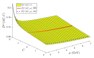
Figure 1: The four-loop prediction on D¯ns(Mτ2,C)superscript¯𝐷nssuperscriptsubscript𝑀𝜏2𝐶\bar{D}^{\rm ns}(M_{\tau}^{2},C) for the Adler function using conventional scale setting, which is shown by a light shaded band. The solid line is for the MS¯¯MS\overline{\rm MS}-scheme, and the dashed line is for the MS-scheme.

A graphical representation of D¯ns(Mτ2,C)superscript¯𝐷nssuperscriptsubscript𝑀𝜏2𝐶\bar{D}^{\rm ns}(M_{\tau}^{2},C) as a function of parameters C𝐶C and μ𝜇\mu is given in Fig. 1, in which we have chosen C[2,+2]𝐶22C\in[-2,+2] 111The relation between the C𝐶C-scheme coupling a^Mτsubscript^𝑎subscript𝑀𝜏\hat{a}_{M_{\tau}} and the MS¯¯MS\overline{\rm MS}-scheme coupling aMτsubscript𝑎subscript𝑀𝜏a_{M_{\tau}} ceases to be perturbative and breaks down below C2similar-to𝐶2C\sim-2. Thus in our discussions we shall adopt C2𝐶2C\geq-2. and μ[Mτ,4Mτ]𝜇subscript𝑀𝜏4subscript𝑀𝜏\mu\in\left[M_{\tau},4M_{\tau}\right]. The shaded band shows the four-loop prediction on D¯ns(Mτ2,C)superscript¯𝐷nssuperscriptsubscript𝑀𝜏2𝐶\bar{D}^{\rm ns}(M_{\tau}^{2},C), which has a large scheme-and-scale dependence. Using a proper C𝐶C, the prediction using the C𝐶C-scheme coupling a^μsubscript^𝑎𝜇\hat{a}_{\mu} is equivalent to predictions using some of the familiar schemes; e.g. the solid line in Fig.1 is for the MS¯¯MS\overline{\rm MS}-scheme and the dashed line is for the MS-scheme. To ensure the equivalence, the value of C𝐶C should be changed for different scales. By taking C=0.188𝐶0.188C=-0.188 one obtains the conventional MS¯¯MS\overline{\rm MS} prediction for μ=Mτ𝜇subscript𝑀𝜏\mu=M_{\tau}; alternatively it can taken as C=0.004𝐶0.004C=-0.004 for μ=4Mτ𝜇4subscript𝑀𝜏\mu=4M_{\tau}.

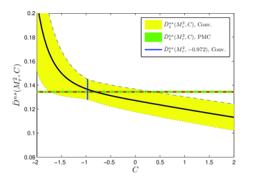
Requiring the estimated “unknown” high-order contribution, |c^n(μ/Mτ)a^μn|MAXsubscriptsubscript^𝑐𝑛𝜇subscript𝑀𝜏superscriptsubscript^𝑎𝜇𝑛MAX|\hat{c}_{n}(\mu/M_{\tau})\hat{a}_{\mu}^{n}|_{\rm MAX}, to be at its minimum, we can obtain an optimal C𝐶C-scheme for D¯nns(Q2,C)superscriptsubscript¯𝐷𝑛nssuperscript𝑄2𝐶\bar{D}_{n}^{\rm ns}(Q^{2},C). At the four-loop level with n=4𝑛4n=4, the optimal C𝐶C-value is 0.9720.972-0.972, leading to

D¯4ns(Mτ2,C=0.972)|Conv.=0.1365±0.0069±0.0083,evaluated-atsubscriptsuperscript¯𝐷ns4superscriptsubscript𝑀𝜏2𝐶0.972Convplus-or-minus0.13650.00690.0083\bar{D}^{\rm ns}_{4}(M_{\tau}^{2},C=-0.972)|_{\rm Conv.}=0.1365\pm 0.0069\pm 0.0083,

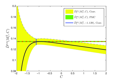
where the central value is for μ=Mτ𝜇subscript𝑀𝜏\mu=M_{\tau}, the first error is for ΔαsMS¯(MZ)=±0.0011Δsuperscriptsubscript𝛼𝑠¯MSsubscript𝑀𝑍plus-or-minus0.0011\Delta\alpha_{s}^{\overline{\rm MS}}(M_{Z})=\pm 0.0011 and the second error is an estimate of the “unknown” high-order contribution. As for a five-loop prediction, if using r5283similar-to-or-equalssubscript𝑟5283r_{5}\simeq 283, the optimal C𝐶C-value changes to 1.1291.129-1.129, and we obtain
D¯5ns(Mτ2,C=1.129)|Conv.=0.1338±0.0062±0.0054.evaluated-atsubscriptsuperscript¯𝐷ns5superscriptsubscript𝑀𝜏2𝐶1.129Convplus-or-minus0.13380.00620.0054\bar{D}^{\rm ns}_{5}(M_{\tau}^{2},C=-1.129)|_{\rm Conv.}=0.1338\pm 0.0062\pm 0.0054.

III.1.2 Predictions using PMC scale-setting

Following the standard PMC-s procedures, by resumming all the RG-involved non-conformal {βi}subscript𝛽𝑖\{\beta_{i}\}-terms into the running coupling, we obtain

D¯nns(Q2,C)|PMC=34i=1nγinsa^Qi.evaluated-atsubscriptsuperscript¯𝐷ns𝑛superscript𝑄2𝐶PMC34superscriptsubscript𝑖1𝑛subscriptsuperscript𝛾ns𝑖superscriptsubscript^𝑎subscript𝑄𝑖\bar{D}^{\rm ns}_{n}(Q^{2},C)|_{\rm PMC}=\frac{3}{4}\sum_{i=1}^{n}\gamma^{\rm ns}_{i}\hat{a}_{Q_{\star}}^{i}. (31)

Using the known four-loop pQCD prediction D¯4nssubscriptsuperscript¯𝐷ns4\bar{D}^{\rm ns}_{4}, the PMC scale Qsubscript𝑄Q_{\star} can be determined up to next-to-next-to-leading log (N2LL) accuracy:

lnQ2Q2=C+0.22493.1382a^Q13.3954a^Q2,superscriptsubscript𝑄2superscript𝑄2𝐶0.22493.1382subscript^𝑎subscript𝑄13.3954superscriptsubscript^𝑎subscript𝑄2\ln\frac{Q_{\star}^{2}}{Q^{2}}=-C+0.2249-3.1382\hat{a}_{Q_{\star}}-13.3954\hat{a}_{Q_{\star}}^{2}, (32)

in which the value of the C𝐶C-scheme coupling a^Qsubscript^𝑎subscript𝑄\hat{a}_{Q_{\star}} can be determined by Eq.(24).

Refer to caption
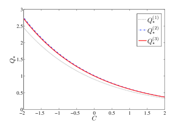
Figure 2: The PMC scale Q(i)subscriptsuperscript𝑄𝑖Q^{(i)}_{\star} of D¯4ns(Mτ2,C)superscriptsubscript¯𝐷4nssuperscriptsubscript𝑀𝜏2𝐶\bar{D}_{4}^{\rm ns}(M_{\tau}^{2},C) as a function of parameter C𝐶C, where i𝑖i indicates the scale is at the N(i-1)LL accuracy.

The PMC scale Qsubscript𝑄Q_{\star} is independent of the choice of the initial scale, which depends on C𝐶C. We present Qsubscript𝑄Q_{\star} as a function of C𝐶C in Fig.2, in which Q(1,2,3)subscriptsuperscript𝑄123Q^{(1,2,3)}_{\star} are at the LL, NLL and N2LLsuperscriptN2LL{\rm N^{2}LL} level, respectively. Fig.2 shows Q(1,2,3)subscriptsuperscript𝑄123Q^{(1,2,3)}_{\star} decreases with the increment of C𝐶C, and Q(1)>Q(2)>Q(3)subscriptsuperscript𝑄1subscriptsuperscript𝑄2subscriptsuperscript𝑄3Q^{(1)}_{\star}>Q^{(2)}_{\star}>Q^{(3)}_{\star}. The optimal scale Qsubscript𝑄Q_{\star} is of perturbative nature: when more loop terms are included, it becomes more accurate. Eq.(24) shows that the C𝐶C-scheme coupling is independent to the choice of C𝐶C. By taking Q=Mτ𝑄subscript𝑀𝜏Q=M_{\tau}, we obtain a^Q0.1056(41)subscript^𝑎subscript𝑄0.105641\hat{a}_{Q_{\star}}\equiv 0.1056(41) for any choice of C𝐶C, where the errors are from ΔαsMS¯(MZ)=±0.0011Δsuperscriptsubscript𝛼𝑠¯MSsubscript𝑀𝑍plus-or-minus0.0011\Delta\alpha_{s}^{\overline{\rm MS}}(M_{Z})=\pm 0.0011. We then obtain the scheme-independent PMC prediction on D¯4nssuperscriptsubscript¯𝐷4ns\bar{D}_{4}^{\rm ns},

D¯4ns(Mτ2,C)|PMC=0.1345±0.0066±0.0008,evaluated-atsuperscriptsubscript¯𝐷4nssuperscriptsubscript𝑀𝜏2𝐶PMCplus-or-minus0.13450.00660.0008\displaystyle\bar{D}_{4}^{\rm ns}(M_{\tau}^{2},C)|_{\rm PMC}=0.1345\pm 0.0066\pm 0.0008, (33)

where the first error is for ΔαsMS¯(MZ)=±0.0011Δsuperscriptsubscript𝛼𝑠¯MSsubscript𝑀𝑍plus-or-minus0.0011\Delta\alpha_{s}^{\overline{\rm MS}}(M_{Z})=\pm 0.0011 and the second error is an estimate of the “unknown” high-order contribution.
Refer to caption
Refer to caption
Figure 3: D¯ns(Mτ2,C)superscript¯𝐷nssuperscriptsubscript𝑀𝜏2𝐶\bar{D}^{\rm ns}(M_{\tau}^{2},C) for the Adler function as a function of the parameter C𝐶C. The solid line is the prediction using conventional scale setting, the lighter-shaded band is the uncertainty for a four-loop prediction Δ=±|c^4(μ/Mτ)a^μ4|MAXΔplus-or-minussubscriptsubscript^𝑐4𝜇subscript𝑀𝜏superscriptsubscript^𝑎𝜇4MAX\Delta=\pm|\hat{c}_{4}(\mu/M_{\tau})\hat{a}_{\mu}^{4}|_{\rm MAX} (Upper) and for an approximate five-loop prediction Δ=±|c^5(μ/Mτ)a^μ5|MAXΔplus-or-minussubscriptsubscript^𝑐5𝜇subscript𝑀𝜏superscriptsubscript^𝑎𝜇5MAX\Delta=\pm|\hat{c}_{5}(\mu/M_{\tau})\hat{a}_{\mu}^{5}|_{\rm MAX} (Lower), where MAX is the maximum value for μ[Mτ,4Mτ]𝜇subscript𝑀𝜏4subscript𝑀𝜏\mu\in[M_{\tau},4M_{\tau}]. When C=0.972𝐶0.972C=-0.972 (Upper) and C=1.129𝐶1.129C=-1.129 (Lower), the error bar as shown by a vertical solid line is the minimum. The dash-dot line represents the four-loop PMC prediction, and the darker shaded band is for Δ=±|r4,0a^Q4|Δplus-or-minussubscript𝑟40subscriptsuperscript^𝑎4subscript𝑄\Delta=\pm|r_{4,0}\hat{a}^{4}_{Q_{\star}}| .

In order to compare the scheme dependence before and after applying the PMC, we present the predictions for D¯ns(Mτ2,C)superscript¯𝐷nssuperscriptsubscript𝑀𝜏2𝐶\bar{D}^{\rm ns}(M_{\tau}^{2},C) for μ=Mτ𝜇subscript𝑀𝜏\mu=M_{\tau} in Fig. 3. At four-loop level, Fig. 3 shows that the scheme-dependence of D¯4ns(Mτ2,C)|Conv.evaluated-atsubscriptsuperscript¯𝐷ns4superscriptsubscript𝑀𝜏2𝐶Conv\bar{D}^{\rm ns}_{4}(M_{\tau}^{2},C)|_{\rm Conv.} is rather large, which decreases with increasing values for C𝐶C; for larger C𝐶C values, the error band becomes slightly larger. When C=0.972𝐶0.972C=-0.972, the error bar is the minimum, corresponding to the optimal scheme. By using the approximate five-loop term r5283similar-to-or-equalssubscript𝑟5283r_{5}\simeq 283, we also give the results for the approximate five-loop prediction. Fig. 3 shows a smaller error bar is achieved with a five-loop term, D¯5ns(Mτ2,C)|Conv.evaluated-atsubscriptsuperscript¯𝐷ns5superscriptsubscript𝑀𝜏2𝐶Conv\bar{D}^{\rm ns}_{5}(M_{\tau}^{2},C)|_{\rm Conv.} first increases and then decreases with the increment of C𝐶C, and the optimal scheme is slightly shifted to C=1.129𝐶1.129C=-1.129. It is interesting to find that the predicted D¯ns(Mτ2,C)|Conv.evaluated-atsuperscript¯𝐷nssuperscriptsubscript𝑀𝜏2𝐶Conv\bar{D}^{\rm ns}(M_{\tau}^{2},C)|_{\rm Conv.} with the optimal choice of C𝐶C are consistent with the PMC predictions within errors. This indicates that the differences caused by various scale-setting approaches could be smeared by including more and more loop terms and be consistent with the scheme-independent predictions. The flat dash-dot line in Fig. 3 shows that the conventional scheme dependence can be eliminated by applying the PMC. Due to the much faster pQCD convergence after applying the PMC, and due to the elimination of the scale dependence, the PMC suggests that the unknown high-order contribution could be quite small in comparison to the present four-loop prediction.

Table 1: The value of each loop-term, LO, NLO, N2LO, or N3LO, for the four-loop prediction D¯4nssubscriptsuperscript¯𝐷ns4\bar{D}^{\rm ns}_{4} using conventional (Conv.) and PMC scale-settings, respectively. μ=Q=Mτ𝜇𝑄subscript𝑀𝜏\mu=Q=M_{\tau}. The results for the MS¯¯MS\overline{\rm MS}-scheme and the optimal C𝐶C-scheme with C=0.972𝐶0.972C=-0.972 are presented. The PMC prediction is unchanged for any C𝐶C-scheme.
 LO  NLO  N2LO  N3LO  Total
 Conv., MS¯¯MS\overline{\rm MS}-scheme 0.1006 0.0166 0.0064 0.0050 0.1286
 Conv., optimal C𝐶C-scheme 0.1347 0.00990.0099-0.0099 0.0034 0.0083 0.1365
 PMC, any C𝐶C-scheme 0.1056 0.0240 0.0041 0.0008 0.1345

We present the value of each loop-term, LO, NLO, N2LO, or N3LO, for the four-loop prediction D¯4nssubscriptsuperscript¯𝐷ns4\bar{D}^{\rm ns}_{4} using conventional and PMC scale-settings in Table 1. The pQCD convergence for the conventional MS¯¯MS\overline{\rm MS}-scheme is moderate. The pQCD convergence for the optimal C𝐶C-scheme (C=0.972𝐶0.972C=-0.972) does not suffer from the usual αssubscript𝛼𝑠\alpha_{s}-suppression, the relativity of the related high-loop terms show, |D¯4ns,LO||D¯4ns,NLO||D¯4ns,N2LO||D¯4ns,N3LO|much-greater-thansubscriptsuperscript¯𝐷nsLO4subscriptsuperscript¯𝐷nsNLO4similar-tosubscriptsuperscript¯𝐷nssuperscriptN2LO4similar-tosubscriptsuperscript¯𝐷nssuperscriptN3LO4|\bar{D}^{\rm ns,LO}_{4}|\gg|\bar{D}^{\rm ns,NLO}_{4}|\sim|\bar{D}^{\rm ns,N^{2}LO}_{4}|\sim|\bar{D}^{\rm ns,N^{3}LO}_{4}|. On the other hand, by applying the PMC, a much better pQCD convergence is achieved due to the elimination of divergent renormalon-like terms.

III.2 τ𝜏\tau decays to ν+limit-from𝜈\nu+ hadrons

The ratio of the τ𝜏\tau total hadronic branching fraction to its lepton branching fraction can be parameterized as,

Rτsubscript𝑅𝜏\displaystyle R_{\tau} =\displaystyle= Γ(τhadrons+ντ)Γ(τl+ν¯l+ντ)Γ𝜏hadronssubscript𝜈𝜏Γ𝜏𝑙subscript¯𝜈𝑙subscript𝜈𝜏\displaystyle\frac{\Gamma(\tau\rightarrow{\rm hadrons}+\nu_{\tau})}{\Gamma(\tau\rightarrow l+\bar{\nu}_{l}+\nu_{\tau})} (34)
=\displaystyle= 3SEW(|Vud|2+|Vus|2)(1+δ(0)+),3subscript𝑆EWsuperscriptsubscript𝑉𝑢𝑑2superscriptsubscript𝑉𝑢𝑠21superscript𝛿0\displaystyle 3S_{\rm EW}\left(|V_{ud}|^{2}+|V_{us}|^{2}\right)(1+\delta^{(0)}+\cdots),

where SEWsubscript𝑆EWS_{\rm EW} is an electroweak correction, |Vud|subscript𝑉𝑢𝑑|V_{ud}| as well as |Vus|subscript𝑉𝑢𝑠|V_{us}| are CKM matrix elements. The pQCD correction is encoded in δ(0)superscript𝛿0\delta^{(0)} and the ellipsis indicate further small subleading corrections. The pQCD correction up to nthsubscript𝑛thn_{\rm th}-order level reads,

δn(0)(Mτ2,μ)=i=1nci(μ/Mτ)aμi,subscriptsuperscript𝛿0𝑛superscriptsubscript𝑀𝜏2𝜇superscriptsubscript𝑖1𝑛subscript𝑐𝑖𝜇subscript𝑀𝜏superscriptsubscript𝑎𝜇𝑖\displaystyle\delta^{(0)}_{n}(M_{\tau}^{2},\mu)=\sum_{i=1}^{n}c_{i}(\mu/M_{\tau})a_{\mu}^{i}, (35)

where the coefficients cisubscript𝑐𝑖c_{i} for the MS¯¯MS\overline{\rm MS}-scheme up to four-loop level can be found in Refs.Baikov:2008jh ; Beneke:2008ad .

III.2.1 Predictions using conventional scale-setting

Taking μ=Mτ𝜇subscript𝑀𝜏\mu=M_{\tau}, we obtain a four-loop MS¯¯MS\overline{\rm MS}-scheme prediction on δ(0)superscript𝛿0\delta^{(0)} using conventional scale-setting,

δ4(0)(Mτ2,μ=Mτ)|Conv.=0.1930±0.0104±0.0199,evaluated-atsubscriptsuperscript𝛿04superscriptsubscript𝑀𝜏2𝜇subscript𝑀𝜏Convplus-or-minus0.19300.01040.0199\delta^{(0)}_{4}(M_{\tau}^{2},\mu=M_{\tau})|_{\rm Conv.}=0.1930\pm 0.0104\pm 0.0199, (36)

where the first error is for ΔαsMS¯(MZ)=±0.0011Δsuperscriptsubscript𝛼𝑠¯MSsubscript𝑀𝑍plus-or-minus0.0011\Delta\alpha_{s}^{\overline{\rm MS}}(M_{Z})=\pm 0.0011 and the second error is an estimate of the “unknown” high-order contribution. If we use the predicted five-loop term r5283similar-to-or-equalssubscript𝑟5283r_{5}\simeq 283 Beneke:2008ad , we obtain
δ5(0)(Mτ2,μ=Mτ)|Conv.=0.1990±0.0113±0.0151.evaluated-atsubscriptsuperscript𝛿05superscriptsubscript𝑀𝜏2𝜇subscript𝑀𝜏Convplus-or-minus0.19900.01130.0151\delta^{(0)}_{5}(M_{\tau}^{2},\mu=M_{\tau})|_{\rm Conv.}=0.1990\pm 0.0113\pm 0.0151. (37)
Refer to caption
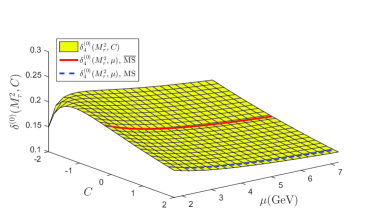
Figure 4: The four-loop prediction on δ(0)(Mτ2,C)superscript𝛿0superscriptsubscript𝑀𝜏2𝐶\delta^{(0)}(M_{\tau}^{2},C) using conventional scale setting, which is shown by a light shaded band. The solid line is for the MS¯¯MS\overline{\rm MS}-scheme, and the dashed line is for the MS-scheme.

The predictions using conventional scale setting are scheme dependent. By using the relation (11), we rewrite δn(0)(Mτ2,μ)subscriptsuperscript𝛿0𝑛superscriptsubscript𝑀𝜏2𝜇\delta^{(0)}_{n}(M_{\tau}^{2},\mu) in terms of the C𝐶C-scheme coupling a^μsubscript^𝑎𝜇\hat{a}_{\mu} as

δn(0)(Mτ2,C)=i=1nc^i(μ/Mτ)a^μi.subscriptsuperscript𝛿0𝑛superscriptsubscript𝑀𝜏2𝐶superscriptsubscript𝑖1𝑛subscript^𝑐𝑖𝜇subscript𝑀𝜏superscriptsubscript^𝑎𝜇𝑖\displaystyle\delta^{(0)}_{n}(M_{\tau}^{2},C)=\sum_{i=1}^{n}\hat{c}_{i}(\mu/M_{\tau})\hat{a}_{\mu}^{i}. (38)

A graphical representation of δ(0)(Mτ2,C)superscript𝛿0superscriptsubscript𝑀𝜏2𝐶\delta^{(0)}(M_{\tau}^{2},C) as a function of parameters C𝐶C and μ𝜇\mu is given in Fig. 4, in which we have chosen C[2,+2]𝐶22C\in[-2,+2] and μ[Mτ,4Mτ]𝜇subscript𝑀𝜏4subscript𝑀𝜏\mu\in\left[M_{\tau},4M_{\tau}\right]. The shaded band shows the four-loop prediction on δ(0)(Mτ2,C)superscript𝛿0superscriptsubscript𝑀𝜏2𝐶\delta^{(0)}(M_{\tau}^{2},C), the solid line is MS¯¯MS\overline{\rm MS}-scheme prediction and the dashed line is the MS-scheme one.

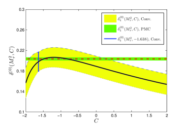
Requiring the approximate “unknown” high-order contribution, |c^n(μ/Mτ)a^μn|MAXsubscriptsubscript^𝑐𝑛𝜇subscript𝑀𝜏superscriptsubscript^𝑎𝜇𝑛MAX|\hat{c}_{n}(\mu/M_{\tau})\hat{a}_{\mu}^{n}|_{\rm MAX}, minimal, we obtain an optimal C𝐶C-scheme for δ(0)(Mτ2,C)superscript𝛿0superscriptsubscript𝑀𝜏2𝐶\delta^{(0)}(M_{\tau}^{2},C) at the nthsubscript𝑛thn_{\rm th}-order level. Using the four-loop prediction with n=4𝑛4n=4, the optimal C𝐶C-value is 1.6381.638-1.638, which leads to

δ4(0)(Mτ2,C=1.638)|Conv.=0.1979±0.0099±0.0186,evaluated-atsubscriptsuperscript𝛿04superscriptsubscript𝑀𝜏2𝐶1.638Convplus-or-minus0.19790.00990.0186\delta^{(0)}_{4}(M_{\tau}^{2},C=-1.638)|_{\rm Conv.}=0.1979\pm 0.0099\pm 0.0186,

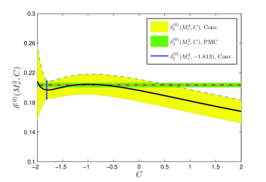
where the first error is for ΔαsMS¯(MZ)=±0.0011Δsuperscriptsubscript𝛼𝑠¯MSsubscript𝑀𝑍plus-or-minus0.0011\Delta\alpha_{s}^{\overline{\rm MS}}(M_{Z})=\pm 0.0011, and the second error is for ±|c^4(μ/Mτ)a^μ4|MAXplus-or-minussubscriptsubscript^𝑐4𝜇subscript𝑀𝜏superscriptsubscript^𝑎𝜇4MAX\pm|\hat{c}_{4}(\mu/M_{\tau})\hat{a}_{\mu}^{4}|_{\rm MAX}. If using the five-loop term r5283similar-to-or-equalssubscript𝑟5283r_{5}\simeq 283, the optimal C𝐶C-value changes to 1.8131.813-1.813, and we obtain

δ5(0)(Mτ2,C=1.813)|Conv.=0.1968±0.0095±0.0118.evaluated-atsubscriptsuperscript𝛿05superscriptsubscript𝑀𝜏2𝐶1.813Convplus-or-minus0.19680.00950.0118\delta^{(0)}_{5}(M_{\tau}^{2},C=-1.813)|_{\rm Conv.}=0.1968\pm 0.0095\pm 0.0118.

III.2.2 Predictions for τ𝜏\tau decay using PMC scale-setting

Up to four-loop level, the known conformal and non-conformal coefficients for conventional coupling can be read from Ref.Brodsky:2013vpa . By resumming all the RG-involved non-conformal {βi}subscript𝛽𝑖\{\beta_{i}\}-terms into the running coupling, we obtain the PMC prediction for δn(0)(Mτ2,C)subscriptsuperscript𝛿0𝑛superscriptsubscript𝑀𝜏2𝐶\delta^{(0)}_{n}(M_{\tau}^{2},C), i.e.

δn(0)(Mτ2,C)|PMC=34i=1nγinsa^Qi,evaluated-atsubscriptsuperscript𝛿0𝑛superscriptsubscript𝑀𝜏2𝐶PMC34superscriptsubscript𝑖1𝑛subscriptsuperscript𝛾ns𝑖superscriptsubscript^𝑎subscript𝑄𝑖\displaystyle\delta^{(0)}_{n}(M_{\tau}^{2},C)|_{\rm PMC}=\frac{3}{4}\sum_{i=1}^{n}\gamma^{\rm ns}_{i}\hat{a}_{Q_{\star}}^{i}, (39)

Using the known four-loop pQCD prediction δ4(0)(Mτ2,C)subscriptsuperscript𝛿04superscriptsubscript𝑀𝜏2𝐶\delta^{(0)}_{4}(M_{\tau}^{2},C), the PMC scale Qsubscript𝑄Q_{\star} can be determined up to next-to-next-to-leading log (N2LL) accuracy:

lnQ2Mτ2=C1.3584+1.6234a^Q1.1385a^Q2,superscriptsubscript𝑄2superscriptsubscript𝑀𝜏2𝐶1.35841.6234subscript^𝑎subscript𝑄1.1385superscriptsubscript^𝑎subscript𝑄2\displaystyle\ln\frac{Q_{\star}^{2}}{M_{\tau}^{2}}=-C-1.3584+1.6234\hat{a}_{Q_{\star}}-1.1385\hat{a}_{Q_{\star}}^{2}, (40)

where the optimal C𝐶C-scheme coupling a^Qsubscript^𝑎subscript𝑄\hat{a}_{Q_{\star}} is determined by Eq.(24).

Refer to caption
Figure 5: The PMC scale Q(i)subscriptsuperscript𝑄𝑖Q^{(i)}_{\star} of δ4(0)(Mτ2,C)subscriptsuperscript𝛿04superscriptsubscript𝑀𝜏2𝐶\delta^{(0)}_{4}(M_{\tau}^{2},C) as a function of parameter C𝐶C, where i𝑖i indicates the scale is at the N(i-1)LL accuracy.

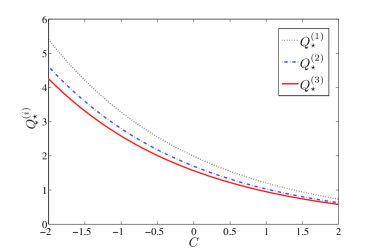
We present the scheme-dependent Qsubscript𝑄Q_{\star} as a function of C𝐶C in Fig.5, in which Q(1,2,3)subscriptsuperscript𝑄123Q^{(1,2,3)}_{\star} are at the LL, NLL and N2LLsuperscriptN2LL{\rm N^{2}LL} level, respectively. To compare with the case of D¯ns(Q2)superscript¯𝐷nssuperscript𝑄2\bar{D}^{\rm ns}(Q^{2}), the perturbative series for lnQ2/Mτ2subscriptsuperscript𝑄2superscriptsubscript𝑀𝜏2\ln{Q^{2}_{\star}}/{M_{\tau}^{2}} oscillates, leading to Q(1)<Q(2)subscriptsuperscript𝑄1subscriptsuperscript𝑄2Q^{(1)}_{\star}<Q^{(2)}_{\star} and Q(2)>Q(3)subscriptsuperscript𝑄2subscriptsuperscript𝑄3Q^{(2)}_{\star}>Q^{(3)}_{\star}; similar to the case of D¯ns(Q2)superscript¯𝐷nssuperscript𝑄2\bar{D}^{\rm ns}(Q^{2}), Q(1,2,3)subscriptsuperscript𝑄123Q^{(1,2,3)}_{\star} decreases with increasing C𝐶C. Eq.(24) indicates the C𝐶C-scheme coupling a^Qsubscript^𝑎subscript𝑄\hat{a}_{Q_{\star}} is free of the parameter C𝐶C, and for the four-loop level we obtain a^Q=0.1449(63)subscript^𝑎subscript𝑄0.144963\hat{a}_{Q_{\star}}=0.1449(63), where the error is for ΔαsMS¯(MZ)=±0.0011Δsuperscriptsubscript𝛼𝑠¯MSsubscript𝑀𝑍plus-or-minus0.0011\Delta\alpha_{s}^{\overline{\rm MS}}(M_{Z})=\pm 0.0011. We then obtain the scheme-and-scale independent PMC prediction on δ4(0)(Mτ2,C)subscriptsuperscript𝛿04superscriptsubscript𝑀𝜏2𝐶\delta^{(0)}_{4}(M_{\tau}^{2},C),

δ4(0)(Mτ2,C)|PMC=0.2035±0.0123±0.0030.evaluated-atsubscriptsuperscript𝛿04superscriptsubscript𝑀𝜏2𝐶PMCplus-or-minus0.20350.01230.0030\displaystyle\delta^{(0)}_{4}(M_{\tau}^{2},C)|_{\rm PMC}=0.2035\pm 0.0123\pm 0.0030. (41)

where the first error is for ΔαsMS¯(MZ)=±0.0011Δsuperscriptsubscript𝛼𝑠¯MSsubscript𝑀𝑍plus-or-minus0.0011\Delta\alpha_{s}^{\overline{\rm MS}}(M_{Z})=\pm 0.0011 and the second error is an estimate of the “unknown” high-order contribution.
Refer to caption
Refer to caption
Figure 6: δ(0)(Mτ2,C)superscript𝛿0superscriptsubscript𝑀𝜏2𝐶\delta^{(0)}(M_{\tau}^{2},C) for τ𝜏\tau decay as a function of the parameter C𝐶C. The solid line is the prediction using conventional scale setting, the lighter-shaded band is the uncertainty for a four-loop prediction Δ=±|c^4(μ/Mτ)a^μ4|MAXΔplus-or-minussubscriptsubscript^𝑐4𝜇subscript𝑀𝜏superscriptsubscript^𝑎𝜇4MAX\Delta=\pm|\hat{c}_{4}(\mu/M_{\tau})\hat{a}_{\mu}^{4}|_{\rm MAX} (Upper) and for an approximate five-loop prediction Δ=±|c^5(μ/Mτ)a^μ5|MAXΔplus-or-minussubscriptsubscript^𝑐5𝜇subscript𝑀𝜏superscriptsubscript^𝑎𝜇5MAX\Delta=\pm|\hat{c}_{5}(\mu/M_{\tau})\hat{a}_{\mu}^{5}|_{\rm MAX} (Lower), where MAX is the maximum value for μ[Mτ,4Mτ]𝜇subscript𝑀𝜏4subscript𝑀𝜏\mu\in[M_{\tau},4M_{\tau}]. When C=1.638𝐶1.638C=-1.638 (Upper) and C=1.183𝐶1.183C=-1.183 (Lower), the error bar as shown by a vertical solid line is the minimum. The dash-dot line represents the four-loop PMC prediction, and the darker shaded band is for Δ=±|r4,0a^Q4|Δplus-or-minussubscript𝑟40subscriptsuperscript^𝑎4subscript𝑄\Delta=\pm|r_{4,0}\hat{a}^{4}_{Q_{\star}}| .
Table 2: The value of each loop-term, LO, NLO, N2LO, or N3LO, for the four-loop prediction δ4(0)(Mτ2)subscriptsuperscript𝛿04superscriptsubscript𝑀𝜏2\delta^{(0)}_{4}(M_{\tau}^{2}) using conventional (Conv.) and PMC scale-settings, respectively. μ=Q=Mτ𝜇𝑄subscript𝑀𝜏\mu=Q=M_{\tau}. The results for the MS¯¯MS\overline{\rm MS}-scheme and the optimal C𝐶C-scheme with C=1.638𝐶1.638C=-1.638 are presented. The PMC prediction is unchanged for any C𝐶C-scheme.
 LO  NLO  N2LO  N3LO  Total
 Conv., MS¯¯MS\overline{\rm MS}-scheme 0.1006 0.0526 0.0268 0.0130 0.1930
 Conv., optimal C𝐶C-scheme 0.1873 0.0532 0.02400.0240-0.0240 0.01860.0186-0.0186 0.1979
 PMC, any C𝐶C-scheme 0.1449 0.0451 0.0105 0.0030 0.2035

To compare the scheme dependence before and after applying the PMC, we present the predictions on δ(0)(Mτ2,C)superscript𝛿0superscriptsubscript𝑀𝜏2𝐶\delta^{(0)}(M_{\tau}^{2},C) for μ=Mτ𝜇subscript𝑀𝜏\mu=M_{\tau} in Fig. 6. At four-loop level, Fig. 6 shows that the error band shall first increases and then decreases with increasing C𝐶C; the optimal scheme is obtained for C=1.638𝐶1.638C=-1.638. By using the approximate five-loop term r5283similar-to-or-equalssubscript𝑟5283r_{5}\simeq 283, we give the results for the approximate five-loop prediction. Fig. 6 shows a smaller error bar is achieved with a five-loop term, D¯5ns(Mτ2,C)|Conv.evaluated-atsubscriptsuperscript¯𝐷ns5superscriptsubscript𝑀𝜏2𝐶Conv\bar{D}^{\rm ns}_{5}(M_{\tau}^{2},C)|_{\rm Conv.} oscillates with the increment of C𝐶C, and the optimal scheme is slightly shifted to C=1.813𝐶1.813C=-1.813. Similar to the case of D¯ns(Mτ2,C)|Conv.evaluated-atsuperscript¯𝐷nssuperscriptsubscript𝑀𝜏2𝐶Conv\bar{D}^{\rm ns}(M_{\tau}^{2},C)|_{\rm Conv.}, it is observed that the predicted δ(0)(Mτ2,C)|Conv.evaluated-atsuperscript𝛿0superscriptsubscript𝑀𝜏2𝐶Conv\delta^{(0)}(M_{\tau}^{2},C)|_{\rm Conv.} with the optimal choice of C𝐶C are also consistent with the PMC predictions within errors. The flat dash-dot line in Fig. 6 shows the conventional scheme dependence can be eliminated by applying the PMC. The unknown high-order contribution could be quite small for the present four-loop PMC prediction.

We present the value of each loop-term, LO, NLO, N2LO, or N3LO, for the four-loop prediction δ4(0)subscriptsuperscript𝛿04\delta^{(0)}_{4} using conventional and PMC scale-settings in Table 2. The pQCD convergence for the conventional MS¯¯MS\overline{\rm MS}-scheme is moderate. The pQCD convergence for the optimal C𝐶C-scheme (C=1.638𝐶1.638C=-1.638) does not suffer from the usual αssubscript𝛼𝑠\alpha_{s}-suppression, |δ4(0),LO||δ4(0),NLO||δ4(0),N2LO||δ4(0),N3LO|much-greater-thansubscriptsuperscript𝛿0LO4subscriptsuperscript𝛿0NLO4similar-tosubscriptsuperscript𝛿0superscriptN2LO4similar-tosubscriptsuperscript𝛿0superscriptN3LO4|\delta^{(0),{\rm LO}}_{4}|\gg|\delta^{(0),{\rm NLO}}_{4}|\sim|\delta^{(0),{\rm N^{2}LO}}_{4}|\sim|\delta^{(0),{\rm N^{3}LO}}_{4}|. On the other hand, by applying the PMC, a better pQCD convergence is achieved due to the elimination of divergent renormalon-like terms.

IV Summary

We have shown that the scheme-and-scale ambiguities introduced by conventional scale-setting are unnecessary by combining the single-scale PMC procedure with the newly suggested scheme-independent C𝐶C-scheme coupling. We have demonstrated that using the C𝐶C-scheme, together with the PMC-s scale-setting, leads to perturbative QCD predictions which are independent of the initial renormalization scale and the choice of the renormalization scheme at all orders.

The pQCD predictions based on the PMC satisfy the standard RGI and all the self-consistency conditions of the renormalization group. Because the divergent renormalon terms are eliminated, the convergence of the PMC series depends on conformal coefficients, which are generally more convergent than conventional pQCD series. The resulting PMC-s approach not only makes the implementation and automation of the PMC simpler and more transparent, but it also achieves precise scheme-and-scale independent predictions simultaneously.

This method for eliminating the scale and scheme ambiguities relies heavily on how well we know the precise value and analytic properties of the strong coupling. In conventional RGE, the scale running is entangled with the scheme parameters, which can only be solved perturbatively or numerically. In contrast, the scheme-and-scale running behavior of a C𝐶C-scheme coupling α^ssubscript^𝛼𝑠\hat{\alpha}_{s} can be exactly separated; it satisfies a RGE free of scheme-dependent {βi}subscript𝛽𝑖\{\beta_{i}\}-terms. The resulting scheme-independent RGE for the C𝐶C-scheme coupling α^ssubscript^𝛼𝑠\hat{\alpha}_{s} provides scheme-independent predictions.

As we have shown, one can utilize a novel C𝐶C-scheme coupling whose scheme-and-scale running behaviors are governed by a single scheme-independent RGE. The value of the parameter C𝐶C can be chosen to match any conventional renormalization scheme. By using the C𝐶C-scheme coupling instead of conventional coupling, we have demonstrated that the C𝐶C-dependence of the PMC predictions can be eliminated up to any fixed order; since the value of C𝐶C is arbitrary, it means the PMC prediction is independent of any renormalization scheme. Two four-loop PMC examples confirm those observations. Thus combining the C𝐶C-scheme coupling with the PMC-s approach, the resulting predictions become completely independent of the choice of the renormalization scheme and the initial renormalization scale, satisfying all of the conditions of RGI. The PMC procedure thus systematically eliminates the scheme-and-scale ambiguities of pQCD predictions, greatly improving the precision of tests of Standard Model and the sensitivity of collider experiments to new physics.

Acknowledgments: This work was supported in part by the National Natural Science Foundation of China under Grant No.11625520, and the Department of Energy Contract No.DE-AC02-76SF00515. SLAC-PUB-17232.

References

  • (1) M. Beneke, Phys. Rept.  317, 1 (1999).
  • (2) E. Gardi and G. Grunberg, Phys. Lett. B 517, 215 (2001).
  • (3) C. G. Callan, Jr., Phys. Rev. D 2, 1541 (1970).
  • (4) K. Symanzik, Commun. Math. Phys.  18, 227 (1970).
  • (5) A. Petermann, Helv. Phys. Acta 26, 499 (1953).
  • (6) N. N. Bogoliubov and D. V. Shirkov, Dokl. Akad. Nauk SSSR 103, 391 (1955).
  • (7) A. Peterman, Phys. Rept.  53, 157 (1979).
  • (8) X. G. Wu, S. J. Brodsky and M. Mojaza, Prog. Part. Nucl. Phys.  72, 44 (2013).
  • (9) S. J. Brodsky and L. Di Giustino, Phys. Rev. D 86, 085026 (2012).
  • (10) S. J. Brodsky and X. G. Wu, Phys. Rev. D 85, 034038 (2012).
  • (11) S. J. Brodsky and X. G. Wu, Phys. Rev. D 86, 014021 (2012).
  • (12) S. J. Brodsky and X. G. Wu, Phys. Rev. Lett.  109, 042002 (2012).
  • (13) M. Mojaza, S. J. Brodsky and X. G. Wu, Phys. Rev. Lett.  110, 192001 (2013).
  • (14) S. J. Brodsky, M. Mojaza and X. G. Wu, Phys. Rev. D 89, 014027 (2014).
  • (15) S. J. Brodsky and X. G. Wu, Phys. Rev. D 86, 054018 (2012).
  • (16) S. J. Brodsky, G. P. Lepage and P. B. Mackenzie, Phys. Rev. D 28, 228 (1983).
  • (17) M. Gell-Mann and F. E. Low, Phys. Rev.  95, 1300 (1954).
  • (18) S. J. Brodsky and P. Huet, Phys. Lett. B 417, 145 (1998).
  • (19) J. M. Shen, X. G. Wu, B. L. Du and S. J. Brodsky, Phys. Rev. D 95, 094006 (2017).
  • (20) S. J. Brodsky and H. J. Lu, Phys. Rev. D 51, 3652 (1995).
  • (21) J. M. Shen, X. G. Wu, Y. Ma and S. J. Brodsky, Phys. Lett. B 770, 494 (2017).
  • (22) D. Boito, M. Jamin and R. Miravitllas, Phys. Rev. Lett.  117, 152001 (2016).
  • (23) D. J. Gross and F. Wilczek, Phys. Rev. Lett.  30, 1343 (1973).
  • (24) H. D. Politzer, Phys. Rev. Lett.  30, 1346 (1973).
  • (25) W. E. Caswell, Phys. Rev. Lett.  33, 244 (1974).
  • (26) O. V. Tarasov, A. A. Vladimirov and A. Y. Zharkov, Phys. Lett.  B 93, 429 (1980).
  • (27) S. A. Larin and J. A. M. Vermaseren, Phys. Lett. B 303, 334 (1993).
  • (28) T. van Ritbergen, J. A. M. Vermaseren and S. A. Larin, Phys. Lett. B 400, 379 (1997).
  • (29) K. G. Chetyrkin, Nucl. Phys. B 710, 499 (2005).
  • (30) M. Czakon, Nucl. Phys. B 710, 485 (2005).
  • (31) P. A. Baikov, K. G. Chetyrkin and J. H. Kuhn, Phys. Rev. Lett.  118, 082002 (2017).
  • (32) R. M. Corless, G. H. Gonnet, D. E. G. Hare, D. J. Jeffrey and D. E. Knuth, Adv. Comput. Math.  5, 329 (1996).
  • (33) H. Y. Bi, X. G. Wu, Y. Ma, H. H. Ma, S. J. Brodsky and M. Mojaza, Phys. Lett. B 748, 13 (2015).
  • (34) M. Jamin and R. Miravitllas, JHEP 1610, 059 (2016).
  • (35) P. M. Stevenson, Phys. Lett. B 100, 61 (1981).
  • (36) P. M. Stevenson, Phys. Rev. D 23, 2916 (1981).
  • (37) P. M. Stevenson, Nucl. Phys. B 231, 65 (1984).
  • (38) Y. Ma, X. G. Wu, H. H. Ma and H. Y. Han, Phys. Rev. D 91, no. 3, 034006 (2015).
  • (39) X. G. Wu, Y. Ma, S. Q. Wang, H. B. Fu, H. H. Ma, S. J. Brodsky and M. Mojaza, Rept. Prog. Phys.  78, 126201 (2015).
  • (40) C. Patrignani et al. [Particle Data Group], Chin. Phys. C 40, 100001 (2016).
  • (41) S. L. Adler, Phys. Rev. D 10, 3714 (1974).
  • (42) P. A. Baikov, K. G. Chetyrkin, J. H. Kuhn and J. Rittinger, JHEP 1207, 017 (2012).
  • (43) K. G. Chetyrkin, J. H. Kuhn and A. Kwiatkowski, Phys. Rept.  277, 189 (1996).
  • (44) P. A. Baikov, K. G. Chetyrkin and J. H. Kuhn, Phys. Rev. Lett.  104, 132004 (2010).
  • (45) M. Beneke and M. Jamin, JHEP 0809, 044 (2008).
  • (46) P. A. Baikov, K. G. Chetyrkin and J. H. Kuhn, Phys. Rev. Lett.  101, 012002 (2008).