Binarizing Weights Wisely for Edge Intelligence:
Guide for Partial Binarization of Deconvolution-Based Generators

Abstract

This work explores the weight binarization of the deconvolution-based generator in a Generative Adversarial Network (GAN) for memory saving and speedup of image construction on the edge. Our study suggests that different from convolutional neural networks (including the discriminator) where all layers can be binarized, only some of the layers in the generator can be binarized without significant performance loss. Supported by theoretical analysis and verified by experiments, a direct metric based on the dimension of deconvolution operations is established, which can be used to quickly decide which layers in a generator can be binarized. Our results also indicate that both the generator and the discriminator should be binarized simultaneously for balanced competition and better performance during training. Experimental results on CelebA dataset with DCGAN and original loss functions suggest that directly applying state-of-the-art binarization techniques to all the layers of the generator will lead to 2.83$\times$ performance loss measured by sliced Wasserstein distance compared with the original generator, while applying them to selected layers only can yield up to 25.81$\times$ saving in memory consumption, and 1.96$\times$ and 1.32$\times$ speedup in inference and training respectively with little performance loss. Similar conclusions can also be drawn on other loss functions for different GANs.

I Introduction

Generative adversarial networks (GANs), which are spin-offs from conventional convolutional neural networks (CNNs), have attracted much attention in the fields of reinforcement learning, unsupervised learning and also semi-supervised learning [1, 2, 3]. A GAN is composed of two parts: a discriminator and a generator. Usually, discriminators are implemented by convolutional neural networks, while generators are implemented by deconvolutional neural networks. More details about GANs will be presented in Section II-B.

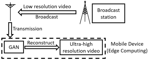
Some promising applications based on GANs include images reconstruction with super-resolution, art creation and image-to-image translation [4], many of which can run on mobile devices (edge computing). For example, one potential application of GANs allow videos to be broadcast in low resolution and then reconstructed to ultra-high resolution by end users [5] as shown in Fig. 1.

Figure 1: Low resolution broadcast based on GAN

However, the resources required by GANs to perform computations in real-time may not be easily accommodated by mobile devices. For example, constructing an image of 64$\times$64 resolution with deep convolutional generative adversarial network (DCGAN) [6] requires 86.6 MB of memory, most of which is used for the generator. The memory goes up to 620.8 MB for 1024$\times$1024 resolution [7], and up to about 800 MB for the popular 4K video with resolution of 3840$\times$2160. On the other hand, one of the state-of-the-art mobile processors, A12 Bionic in the newest iPhone XS Max [8], provides only 4 GB RAM, most of which must be occupied by the operating system and its peripheries. As a result, developers must restrict neural network models to just a few megabytes to avoid crash [9]. The memory budget gets even tighter when it comes to mobile devices of smaller form factor such as Apple Watch series 3, which only has 768 MB RAM.

The same problem has been well known for conventional CNNs, and various solutions have been proposed via redesigning the algorithms and/or computation structures [10, 11, 12, 13]. Among them, quantization until binary is one of the most popular techniques as it fits hardware implementation well with high efficiency [9, 14, 15]. However, quantization can reduce the expressive power of the neural networks significantly and the discrete parameters make the optimization much more difficult. Naive quantization usually leads to total failure especially for binarization. Significant effort has been devoted to develop better quantization and binarization methods as well as the hardware accelerator [16, 14, 17, 18, 19]. Its success on CNNs has been demonstrated by multiple works, where memory consumption is deeply compressed although sometimes the performance cannot be preserved [20, 21, 22, 23].

Compression techniques can be readily applied to discriminator networks in GANs, which are nothing different from conventional CNNs. It may be alluring to also apply the quantization techniques to binarize generators, especially the deconvolution-based [24] ones as the computation process looks similar. However, instead of distilling local information from a global map as in convolution operations, deconvolution attempts to construct the global map by local information. This difference can lead to significantly different binarization results, as will be discussed in Section III. Accordingly, a scheme tailored to deconvolution-based generators is warranted.

In this paper, we show through theoretical analysis that under certain conditions, binarizing a deconvolution layer may cause significant performance loss, which also happens in compression of CNNs per empirical findings so far. Since there is no explanation for this phenomenon to the best of the authors’ knowledge, an intuitive guess is that not all layers can be binarized together while preserving performance. Thus, some layers need to stay in the format of floating point for performance, while others can be binarized without affecting performance. To quickly decide whether a layer can be binarized, supported by theoretical analysis and verified by experiments, a simple yet effective metric based on the dimension of deconvolution operations is established. Based on this metric, we can make use of existing compression techniques to binarize the generator of GANs with little performance loss. We then propose the scheme of partial binarization of deconvolution-based generators (PBGen) under the guide of the metric.

Furthermore, we find that only binarizing the generator and leaving discriminator network unchanged will introduce unbalanced competition and performance degradation. Thus, both networks should be binarized at the same time. Experimental results based on CelebA suggest that directly applying state-of-the-art binarization techniques to all the layers of the generator will lead to 2.83$\times$ performance loss measured by sliced Wasserstein distance compared with the original generator, while applying them to selected layers only can yield up to 25.81$\times$ saving in memory consumption, and 1.96$\times$ and 1.32$\times$ speedup in inference and training respectively with little performance loss. The conclusions will stay the same even though different loss functions are utilized.

The remainder of the paper is organized as follows. Section II discusses related works and background for compression techniques for CNN as well as GANs. Section III exhibits the theoretical analysis on the power of representation in deconvolution/convolution layers and the algorithm for model binarization based on it. Experiments for verification and performance are displayed in Section IV. This work is concluded in Section V.

II Related Works and Background

II-A CNN Compression

Compression techniques for CNNs mainly consist of pruning, quantization, re-structure and other approximations based on mathematical matrix manipulations [10, 25, 26]. The main idea of the pruning method in [21] is to “prune” connections with smaller weights out so that both synapses and neurons are possible to be removed from the original structure. This can work well with traditional CNNs and reduce the number of parameters of AlexNet by a factor of nine [21]. Re-structure methods modify network structures for compression, such as changing functions or block order in layers [26, 20].

In this work, we focus on the quantization technique. Quantization aims to use fewer bits to present values of weights or even inputs. It has been used to accelerate CNNs in various works at different levels [27, 28, 29] including ternary quantization [16, 30] and iterative quantization [31], with small loss. In [10], the authors proposed to determine weight sharing after a network is fully trained, so that the shared weights approximate the original network. From a fully trained model, weights are clustered and replaced by the centroids of clusters. During retraining, the summation of the gradients in same groups are used for the fine-tuning of the centroids. Through such quantization, it is reported to be able to compress AlexNet up by around 8% before significant accuracy loss occurs. If the compression rate goes beyond that, the accuracy will deteriorate rapidly.

A number of recent works [14, 23, 20, 32, 33, 34, 35] pushed it further by using binarization to compress CNNs, where only a single bit is used to represent values. Training networks with weights and activations constrained to $\pm$1 was firstly proposed in [33]. Through transforming 32-bit floating point weight values to binary representation, CNNs with binary weights and activations are about 32$\times$ smaller. In addition, when weight values are binary, convolutions can be estimated by only addition and subtraction without multiplication, which can achieve around 2.0$\times$ speedup. However, the method introduces significant performance loss. To alleviate the problem, [20] proposed Binary-Weight-Network, where all weight values are binarized with an additional continuous scaling factor for each output channel. We will base our discussion on this weight binarization afterwards, which is one of the state-of-the-art binarization methods.

Most recently, hybrid quantization has attracted more and more attention, because it enables better trade-off between compression and performance  [36, 37, 38]. As for partial binarization, a sub-area of hybrid quantization, on which we are focused, both training methods  [39] and the corresponding hardware accelerators [19, 40] are also investigated extensively. The actual performance after compression heavily depends on the configuration of the partial binarization, i.e. which layers are binarized while others are not. Given the fact that the search space is too large to do exhaustive search, finding the optimal or near-optimal configuration becomes a foremost challenge. [41] shows that adding full precision residual connections helps to reduce the loss of classification accuracy while getting excellent memory compression. One potential drawback of this method is that it introduces additional memory overhead. [39] presents flexible network binarization with layer-wise priority, which is defined by the inverse of layer depth empirically. [42] proposes to use the binarization error of each layer as the indication of its importance to the final performance. They empirically show that partial binarization leads to significant improvement over fully binarized models. Very recently, [43] also utilizes Principal Component Analysis (PCA) to identify significant layers in CNNs and uses higher precision on important layers. However, this method depends on pre-trained models, and PCA contains a large amount of computation naturally.

All things considered, none of the existing works explored the compression of generators in GANs, where deconvolution replaces convolution as the major operation. Note that while there is a recent work that uses the term of “binary generative adversarial networks” [44], it is not about the binarization of GANs. In that work, only the inputs of the generator are restricted to binary code to meet the specific application requirement. All parameters inside the networks and the training images are not quantized.

II-B GAN

GAN was developed by [45] as a framework to train a generative model by an adversarial process. In a GAN, a discriminative network (discriminator) learns to distinguish whether a given instance is real or fake, and a generative network (generator) learns to generate realistic instances to confuse the discriminator.

Originally, the discriminator and the generator of a GAN are both multilayer perceptrons. Researchers have since proposed many variants of it. For example, DCGAN transformed multilayer perceptrons to deep convolutional networks for better performance. Specifically, the generator is composed by four deconvolutional layers. GANs with such a convolutional/deconvolutional structure have also been successfully used to synthesize plausible visual interpretations of given text [46] and to learn interpretable and disentangled representation from images in an unsupervised way [47]. Wasserstein generative adversarial networks (WGAN) [48] and least squares generative adversarial networks (LSGAN) [49] have been proposed with different loss functions to achieve more stable performance, yet they both employed the deconvolution operations too. To verify the robustness of our analysis, both DCGAN and LSGAN are tested in our experiments.

III Analysis on Power of Representation

In this section, to decide whether a layer can be binarized, we analyze the power of a deconvolution layer to represent any given mapping between the input and the output, and how such power will affect the performance after binarization. We will show that the performance loss of a layer is related to the dimension of the deconvolution, and develop a metric called the degree of redundancy to indicate the loss. Finally, based on the analysis, several inferences are deduced at the end of this section, which should lead to effective and efficient binarization.

In the discussion below, we ignore batch normalization as well as activation operations and focus on the deconvolution operation in a layer, as only the weights in that operation are binarized. The deconvolution process can be transformed to equivalent matrix multiplication. Let $\mathbf{D}^{I}$ ($\in\mathcal{R}^{{c_{i}}\times{h_{i}}\times{w_{i}}}$, where ${c_{i}}$, ${h_{i}}$ and ${w_{i}}$ are number of channels, height and width of the input respectively) be the input matrix, and $\mathbf{D}^{O}$ ($\in\mathcal{R}^{{c_{o}}\times{h_{o}}\times{w_{o}}}$, where ${c_{o}}$, ${h_{o}}$ and ${w_{o}}$ are the number of channels, height and width of the output respectively) be the output matrix. Denote $\mathbf{K}$ ($\in\mathcal{R}^{{c_{i}}\times{c_{o}}\times{h_{k}}\times{w_{k}}}$, where ${h_{k}}$ and ${w_{k}}$ are the height and width of a kernel in the weight matrix) as the weight matrix to be deconvoluted with $\mathbf{D}^{I}$. Padding is ignored in the discussion, since it will not effect the results.

For the deconvolution operation, the local regions in the output can be stretched out into columns, by which we can cast $\mathbf{D}^{O}$ to $\mathbf{D}^{Od}\in\mathcal{R}^{{s_{i}}\times{r_{o}}}$, where $s_{i}=h_{i}w_{i},r_{o}=c_{o}h_{k}w_{k}$. Similarly, $\mathbf{D}^{Id}\in\mathcal{R}^{{s_{i}}\times{c_{i}}}$ can be restructured from $\mathbf{D}^{I}$, and $\mathbf{K}^{d}\in\mathcal{R}^{c_{i}\times r_{o}}$ can be restructured from $\mathbf{K}$, where $s_{i}=h_{i}w_{i},r_{o}=c_{o}h_{k}w_{k}$. Please refer to [50] for details about the transform. Then, the deconvolution operation can be compactly written as

$$\mathbf{D}^{Od}=\mathbf{D}^{Id}*\mathbf{K}^{d},$$ (1)

where $*$ denotes matrix multiplication. $\mathbf{D}^{Id}$ and $\mathbf{D}^{Od}$ are the matrices containing pixels for an image or an intermediate feature map. During the training process, we adjust the values of $\mathbf{K}^{d}$ to construct a desired mapping between $\mathbf{D}^{Id}$ and $\mathbf{D}^{Od}$.

We use $(\cdot)_{j}$ to denote the $j$-th column of a matrix. Then (1) can be decomposed column-wise as

$$\mathbf{D}^{Od}_{j}=\mathbf{D}^{Id}*\mathbf{K}^{d}_{j},\quad 1\leq j\leq r_{o},$$ (2)

where $\mathbf{K}^{d}_{j}\in\mathcal{R}^{c_{i}}$ and $\mathbf{D}^{Od}_{j}\in\mathcal{R}^{s_{i}}$.

Now we analyze a mapping between an arbitrary input $\mathbf{D}^{Id}$ and an arbitrary output $\mathbf{D}^{Od}_{j}$. From (2), when the weights are continuously selected, all vectors that can be expressed by the right hand expression is a subspace $\Omega$ spanned by the columns of $\mathbf{D}^{Id}$, the dimension of which is $c_{i}$. Here we have assumed without loss of generality that $\mathbf{D}^{Id}$ has full column rank. When $c_{i}<s_{i}$, which is the dimension of the output space $\Phi$ where $\mathbf{D}^{Od}_{j}$ lies, $\Omega$ is of lower dimension than $\Phi$, and accordingly, $\mathbf{D}^{Od}_{j}$ can either be uniquely expressed as a linear combination of the columns in $\mathbf{D}^{Id}$ if it lies in $\Omega$ (i.e. a unique $\mathbf{K}^{d}_{j}$ exists), or cannot be expressed if it is not (i.e. no such $\mathbf{K}^{d}_{j}$ exists). When $c_{i}=s_{i}$, $\Omega$ and $\Phi$ are equivalent, and any $\mathbf{D}^{Od}$ can be uniquely expressed as a linear combination of the columns in $\mathbf{D}^{Id}$. When $c_{i}>s_{i}$, $\Omega$ and $\Phi$ are still equivalent, but any $\mathbf{D}^{Od}$ can be expressed as an infinite number of different linear combinations of the columns in $\mathbf{D}^{Id}$. In fact, the coefficients $\mathbf{K}^{d}_{j}$ of these combinations lie in a $(c_{i}-s_{i})$-dimensional sub-space $\Psi$.

The binarization imposes a constraint on the possible values of the elements in $\mathbf{K}^{d}_{j}$. Only finite number of combinations are possible. If $c_{i}\leq s_{i}$, then at least one of these combinations has to be proportional to the unique $\mathbf{K}^{d}_{j}$ that yields the desired $\mathbf{D}^{Od}_{j}$ to preserve performance. If $c_{i}>s_{i}$, then one of these combinations needs to lie in the subspace $\Psi$ to preserve performance. Apparently, the larger the dimension of $\Psi$ is, the more likely this will happen, and the less the performance loss is. A detailed math analysis is straightforward to illustrate this, and is omitted here in the interest of space. Accordingly, we define the dimension of $\Psi$, $c_{i}-s_{i}$, as the degree of redundancy in the rest of the paper. Note that when this metric is negative, it reflects that $\Omega$ is of lower dimension than $\Phi$ and thus this deconvolution layer is more vulnerable to binarization errors. In general, a higher degree of redundancy should give lower binarization error.

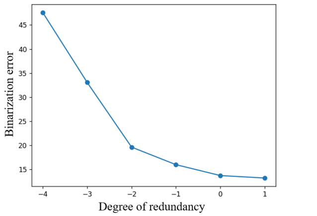
We will use a small numerical example to partially validate the above discussion. We construct a deconvolution layer and vary its degree of redundancy by adjusting the $c_{i}$ in it, where $s_{i}=20$. For each degree of redundancy we calculate the minimum average Euclidean distance between the original output and the output produced by binarized weights, which reflects the error introduced through the binarization process, referred to as binarization error throughout the paper. The binarization error is obtained by enumerating all the possible combinations of those binary weights. The results are depicted in Fig. 2. From the figure we can see that the error decreases with the increase of degree of redundancy, which matches our conjecture.

Figure 2: Binarization error v.s. degree of redundancy for a deconvolution layer

Figure 3: Degree of redundancy v.s. layer number for DCGAN. The intermediate feature maps at the output of each layer as well as the final output are also presented

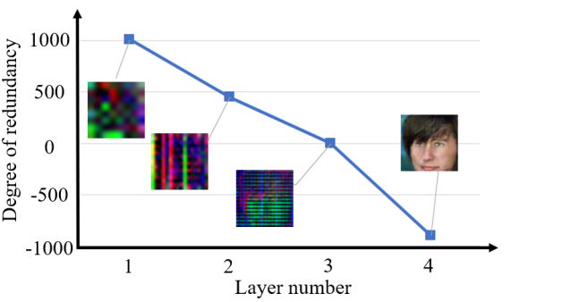
For generators in most state-of-the-art GAN models [6, 49], we find that the degree of redundancy reduces with the increase in depth, eventually dropping below zero. Such a decrease reflects the fact that more details are generated at the output of a layer as its depth grows, as can also be seen in Fig. 3. These details are highly correlated, and reduce the subspace needed to cover then.

Based on our analysis, several inferences can be deduced to guide the binarization:

• With the degree of redundancy, taking advantage of existing binarization methods becomes reasonable and feasible. Binarizing layers with higher degree of redundancy will lead to lower performance loss after binarization, while layers with negative degree of redundancy should be kept un-binarized to avoid excessive performance loss.

• According to the chain rule of probability in directed graphs, the output of every layer is only dependent on its direct input. Therefore, the binarizability of each layer can be superposed. If a layer can be binarized alone, it can be binarized with other such layers.

• When binarizing several deconvolution layers together, the layer with the least degree of redundancy may be the bottleneck of the generator’s performance.

As a result, only shallower layer(s) of a generator can be binarized together to preserve its performance, because of the degree of redundancy trend in it. This leads to PBGen. Besides, such analysis may also explain why binarization can be applied in almost all convolution layers: distilling local information from a global map leads to positive degree of redundancy.

Under the guide of such inferences, the algorithm for wise binarization on Deconv/Conv networks can be implemented by calculating the degree of redundancy for every Deconv/Conv layer at first; then all these layers can be sorted by their degree of redundancy from high to low; in this order, every layer will be binarized singly to observe the difference in performance from the original full-precision version and whether to continue or not will be decided by the trade-off between performance and efficiency; finally, selected layers will be binarized together to serve as the ultimate strategy for network binarization. This algorithm can be described as Algorithm 1. We attempt to preserve the original full-precision performance in our experiments.

Algorithm 1 Wise binarization on Deconv/Conv networks

  $L\leftarrow$ number of Deconv/Conv layers

  $T\leftarrow$ performance degradation threshold

  for $l=1:L$ do

     Compute the degree of redundancy of each layer $R_{l}$

  end for

  $\mathbf{R}\leftarrow\$sorted $R_{1}\cdots,R_{L}$ from high to low

  $i\leftarrow 1$

  while $i\leq L$ do

     Binarize the $i$-th layer

     if performance degradation exceeds $T$ then

        break

     end if

     $i\leftarrow i+1$

  end while

  return  $i$

  The network binarization strategy is to binarize the first $i-1$ layers according to $\mathbf{R}$ together

In addition, following the same derivation process for deconvolution in our manuscript, the degree of redundancy of a convolution layer can be defined as $w_{k}\times h_{k}\times c_{i}-c_{o}$, instead of $c_{i}-s_{i}$ for deconvolution. Usually in a convolution layer, $c_{o}=2\times c_{i}$, $w_{k}=h_{k}$, and $w_{k}=3$ or $5$. As a result, the degree of redundancy is usually positive, and convolution is more readily binarizable compared to deconvolution as well. This also explains why using $1\times 1$ kernels will help compress networks while not hurting the networks’ performance [51].

Figure 4: Structure of the generators in DCGAN with dimension of each layer labeled. Deconvolutional layers are denoted as “CONV” (figure credit: [6])

IV Experiments

IV-A DCGAN and Different Settings

DCGAN will serve as a vehicle to verify the inferences deducted from the theoretical analysis in Section III. Except for the original adversarial loss function for DCGAN, least square loss function proposed in LSGAN is also tested in our experiments. The least square loss is one of the most popular loss functions for GANs, because it has been proved to be efficient for different GANs training.

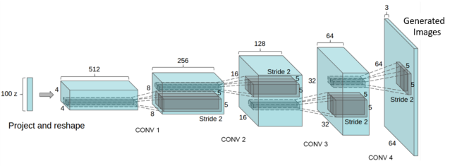
We will explore how to best binarize it with preserved performance. Specifically, we use the TensorFlow [52] implementation of DCGAN on GitHub [53]. The structure of its generator is illustrated in Fig. 4. The computed degree of redundancy in each layer in the generator is shown in Fig. 3 and qualitatively summarized in TABLE I. The degree of redundancy in the last layer drops to -960. According to the inferences before, we can expect that since the degree of redundancy decreases as the depth increases, binarizing shallower layers and keeping the deeper layers in the format of floating point will help preserve the performance. For the readers’ information, the degrees of redundancy of the four convolution layers in the discriminator are 11, 1472, 2944, and 5888 respectively.

TABLE I: Degree of redundancy in each deconvolution layer of the generator in DCGAN

Layer number	Label in Fig. 4	Degree of redundancy
1	CONV 1	496
2	CONV 2	192
3	CONV 3	-128
4	CONV 4	-960

The binarization method used in Binary-Weight-Networks (BWN) proposed in [20] is adopted to binarize layers no matter in a generator network or in a discriminator network. In BWN, all the weight values are approximated with binary values. Through keeping floating-point gradients while training, BWN is able to trained from scratch without pre-train.

There are four deconvolution layers in total in the generator, and each layer can be either binarized or not. For verification, we have conducted experiments on all $2^{4}=16$ different settings, but only the eight representative ones are discussed for clarity and space, and others will lead us to the same conclusion. Those eight different representative settings are summarized in TABLE II for clearness. In this table, the “Setting” column labels each setting. “Layer(s) binarized” indicates which layer(s) are binarized in the generator. The “Discriminator binarized” column tells whether the discriminator is binarized or not. “Y” means yes, while “N” means no. This column is introduced to verify an observation in our experiments to be discussed later. Although settings in experiments include unbinarized discriminator and binarized discriminator, whether the discriminator is binarized or not will not affect the generated images significantly. That is, if the generator cannot generate recognizable faces with the unbinarized discriminator, it still cannot generate any recognizable faces with a binarized discriminator; and vice versa.

TABLE II: Settings of different partial binarization of generator in DCGAN

Setting	Layer(s) binarized	Discriminator binarized
A	None	N
B	1	N
C	2	N
D	3	N
E	4	N
F	1,2,3	N
G	1,2,3,4	N
H	1,2,3	Y

Setting G will serve as the baseline model for performance after binarization, because it adopts the compression techniques based on CNNs directly without considering the degree of redundancy. On the other hand, Setting A serves as the baseline model when considering the memory saving, speedup as well as performance difference before and after binarization, because it represents the original DCGAN in floating point representation. It is considered as one common GAN structure providing good performance.

IV-B Dataset and Metrics

CelebA [54] is used as the dataset for our experiments, because it is a popular and verified dataset for different GAN structures. DCGAN, WGAN, LSGAN and many other GAN structures are tested on it [55]. As every image in CelebA contains only one face, it is much easier to tell the quality of the generated images.

Traditionally the quality of the generated images is identified by observation. However, qualitatively evaluation is always a hard problem. According to the in-depth analysis of commonly used criteria in [56], good performance in a single or extrapolated metric from average log-likelihood, Parzen window estimates, and visual fidelity of samples does not directly translate to good performance of a GAN. On the other hand, the log-likelihood score proposed in [57] only estimates a lower bound instead of the actual performance.

(a) Setting A

(b) Setting B

(c) Setting C

(d) Setting D

(e) Setting E

(f) Setting F

(g) Setting G

(h) Setting H

Figure 5: Images generated under different settings

Very recently, [7] proposed an efficient metric, which we will use in our experiments, and showed that it is superior to MS-SSIM [58], which is a commonly used metric. It calculates the sliced Wasserstein distance (SWD) between the training samples and the generated images under different resolutions. In particular, the SWD from the lower resolution patches indicates similarity in holistic image structures, while the finer-level patches encode information about pixel-level attributes. In this work, the max resolution is 64$\times$64. Thus, according to [7], we will use three different resolutions to evaluate the performance: 16$\times$16, 32$\times$32, and 64$\times$64. For all different resolutions, small SWD indicates that the distributions of the patches are similar, which means that a generator with smaller SWD is expected to produce images more similar to the images from the training samples in both appearance and variation.

IV-C Experimental Results

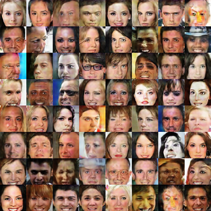
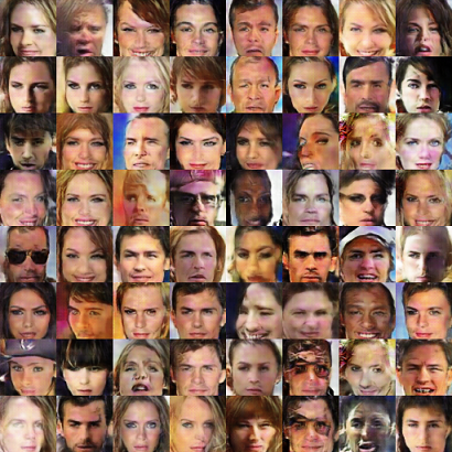
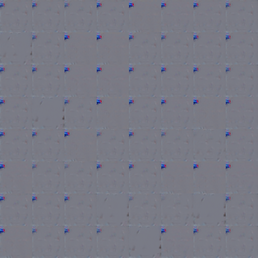
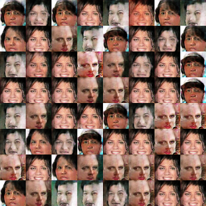
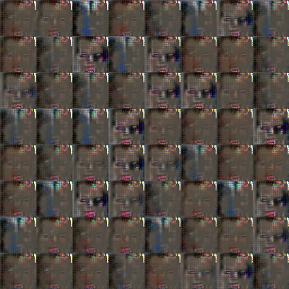
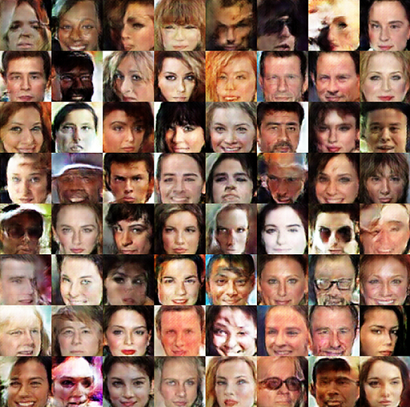
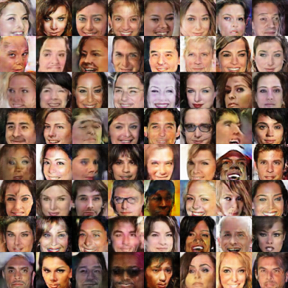
In this section, we will present experimental results that verify our inferences in Section III, along with some additional observations about the competition between the generator and the discriminator. The images generated by the original GAN (Setting A), in which all weights of each deconvolution layer are in the form of floating point, are displayed in Fig. 5a. The images generated by the binarized DCGAN without considering the degree of redundancy are displayed in Fig. 5g. These are our two baseline models.

IV-C1 Qualitative Comparison of Single-Layer Binarization

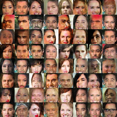
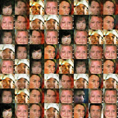
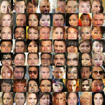
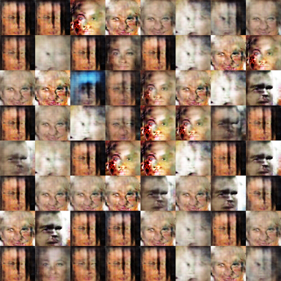
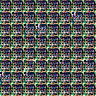
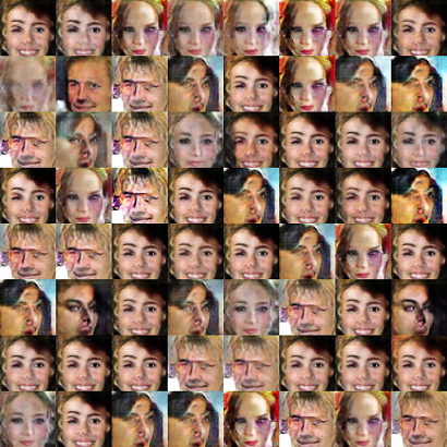
We start our experiments by comparing the images generated by binarizing a single layer in the generator of DCGAN. The results are shown in Figures 5b - 5e, which are generated by PBGen’s under Setting B - Setting E respectively. In other words, those PBGen’s utilize binary weights to the first, the second, the third, and the last deconvolution layer respectively. The degree of redundancy of each layer is shown in Fig. 3. From the generated figures we can then see that Fig. 5b generates the highest quality of images, similar to the original ones in Fig. 5a. Images in Fig. 5c are slightly inferior to those in Fig. 5b, but better than those in Fig. 5d. Fig. 5e has no meaningful images at all. These observations are in accordance with our inferences in Section III: the performance loss when binarizing a layer is decided by its degree of redundancy, and a layer with negative degree of redundancy should not be binarized.

Figure 6: SWD v.s degree of redundancy of the binarized layer in different settings

To address the concern that low performance of Setting E is caused by the low degree of redundancy instead of the position of the layer (the last layer), more experiments are conducted under Setting E. As analysed in Section III, degree of redundancy is defined by $c_{i}-s_{i}$, thus changing $c_{i}$ of one layer will only change the degree of redundancy of that layer, and will not have an effect on other layers’ degree of redundancy. Thus, experiments with different number of input channels for the CONV4 layer, $c_{4}$, under Setting E. The generated images of faces in these experiments are shown in Fig. 7. The original $c_{4}$ is 64, and experiments are also conducted with 128, 256, 512, and 1024 respectively. According to TABLE I, the degree of redundancy of CONV4 is zero when $c_{4}=1024$. As shown in Fig. 7, the generated images get clearer with more details along with the increased number of input channels and higher degree of redundancy.

(a) 64

(b) 128

(c) 256

(d) 512

(e) 1024

Figure 7: Generated images of faces under Setting E with different number of input channels for the CONV4 layer. The number of the CONV4 layer for each experiments is (a) 64, (b) 128, (c) 256, (d) 512, and (e) 1024 respectively. With the increased number of input channels in the CONV4 layer, the degree of redundancy of this layer increases while other layers’ degree of redundancy stays the same. This validates the degree of redundancy as an indication of the capability for a layer.

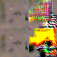
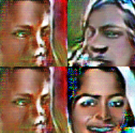
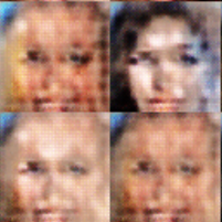
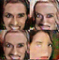
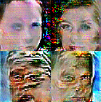
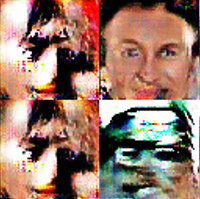
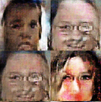
In addition, we also conducted the experiments that vary the DOR of the first three layers when binarizing the fourth layer to validate that every layer binarization is relatively independent. In fact, none of these experiments could achieve the same performance improvement as that when increasing the DOR of the fourth layer by a same number. Generated images are shown in Fig. 8.

(a) None

(b) CONV1

(c) CONV2

(d) CONV3

(e) CONV4

Figure 8: Generated images of faces after binarizing the CONV4 layer. The layer with increased DOR for each experiment is (a) none, (b) CONV1, (c) CONV2, (d) CONV3, and (e) CONV4 respectively. The DOR is increased by 960 for each experiment except for (a). We can see that increasing the DOR of other layers cannot solve the bottleneck problem introduced by CONV4, but increasing the DOR of CONV4 can.

IV-C2 Quantitative Comparison of Single-Layer Binarization

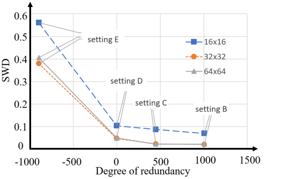
We further quantitatively compute the SWD values with 16$\times$16, 32$\times$32 and 64$\times$64 resolutions for Setting B, Setting C, Setting D, and Setting E. Their relationship with the degree of redundancy of the binarized layer is plotted in Fig. 6. From the figure, two things are clear: first, regardless of resolution, a negative degree of redundancy (Setting E) results in a more than 5$\times$ increase in SWD compared with other settings with non-negative degree of redundancy (Setting B, Setting C, and Setting D). Second, for all the three resolutions, SWD decreases almost linearly with the increase of the degree of redundancy when it is non-negative. This confirms that our degree of redundancy can capture the impact of binarization not only on the holistic structure but also on the pixel-level fine details, and as such, is indeed a good indicator to quickly judge whether a layer can be binarized.

We also report the SWD averaged over different resolutions (16$\times$16, 32$\times$32, 64$\times$64) in TABLE III, where the result for the original GAN (Setting A) is also reported. From the table we can draw similar conclusions, that binarizing second layer (Setting C) increases the average SWD by 2.3% compared with the original GAN (Setting A), while binarizing third and fourth layer (Setting D and Setting E) further increases it by 52.3% and 913.6%, respectively.

Figure 9: SWD v.s. resolution for SWD score calculation under Setting A and Setting B

TABLE III: Average SWD under different settings

Setting	A	B	C	D	E
Average SWD ($\times 10^{-3}$)	44	38	45	67	449

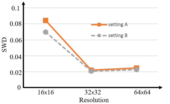
It is interesting to note that the average SWD achieved by binarizing the first layer (Setting B) is 13.6% smaller than that from the original DCGAN (Setting A). To further check this, we plot the SWD v.s. resolution for these two settings in Fig. 9. From the figure we can see that the SWD from Setting B is always smaller than that from Setting A across all three resolutions. This shows that Setting B can achieve better similarity as well as detailed attributes. Such an improvement is probably due to the regularization effect, and similar effect has been observed in the compression of CNNs [32].

(a) Setting A

(b) Setting B

(c) Setting C

(d) Setting D

(e) Setting E

(f) Setting F

(g) Setting G

(h) Setting H

Figure 10: Images generated under different settings using the least square loss

IV-C3 Validation of Superposition of Binarizability

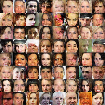
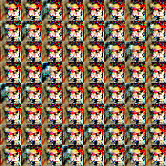
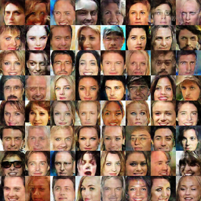
We now explore experiments to verify our inference that all layers that can be binarized alone can be binarized together. The images generated by Setting F in Fig. 5f, where the first three layers in the generator are binarized together, show no significant difference from those in Figures 5a- 5d. Binarizing any two layers from the first three layers (not shown here) will lead to the same result. On the other hand, Setting G does not generate any meaningful output (Fig. 5g), as the last layer, which cannot be binarized alone, is binarized together with the first three layers. Binarizing any of the first three layers as well as the last layer (not shown here) will produce meaningless results too. Setting G follows the state-of-the-art binarization for CNNs directly without considering the degree of redundancy. That is, with the assistance of the degree of redundancy, we can figure out that at most the first three deconvolution layers can be binarized with small loss on performance in the generator (Setting F). Nevertheless, directly adopting the existing binarization method will lead to excess degradation in performance and cannot provide any hint to improve (Setting G).

Figure 11: SWD v.s. resolutions under Setting D and Setting F

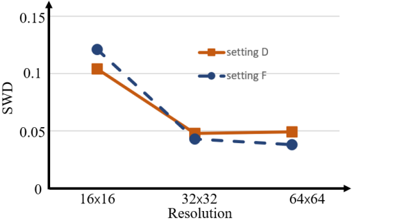
Moreover, the average SWD for Setting F is 0.067, the same as Setting D. Further looking at the SWD values under different resolutions for the two different settings as shown in Fig. 11, it is clear that the two curves are very close. This validates our last inference, that when multiple layers are binarized together, the layer with least degree of redundancy is the bottleneck, which decides the overall performance of the network.

IV-C4 Experimental Results Using the Least Square Loss

The experiments using the least square loss resulted are in accord with our previous experimental results as well as conclusions.

For each layer, the performance after binarization decreases along with the layer’s redundancy. The images generated by binarizing a single layer in the generator after training using the least square loss are shown in the Fig. 10. Same as in Fig. 5, Fig. 10a displays the original results using the least square loss. Figures 10b - 10e are generated by PBGen’s under Setting B - Setting E respectively using the least square loss. As mentioned before, the degree of redundancy of each layer is shown in Fig. 3, which decreases along each layer. As a result, the quality of the generated images also decreases along binarizing each layer under Setting B, Setting C, Setting D, and Setting E. This is the same as that observed in the experiments based on the original loss function in DCGAN.

The superposition of binarizability also holds in the experiments based on the least square loss. The images generated by Setting F in Fig. 10f, where the first three layers in the generator are binarized together, show no significant difference from those in Figures 10a- 10d. Binarizing any two layers from the first three layers (not shown here) will lead to a similar result. On the other hand, Setting G does not generate any meaningful output (Fig. 10g), as the last layer, which cannot be binarized alone, is binarized together with the first three layers. Binarizing any of the first three layers as well as the last layer (not shown here) will produce meaningless results too. Setting G follows the state-of-the-art binarization for CNNs directly without considering the degree of redundancy based on the least square loss. That is, with the assistance of the degree of redundancy, we can figure out that at most the first three deconvolution layers can be binarized with small loss on performance in the generator (Setting F) even based on the least square loss in DCGAN. Nevertheless, directly adopting the existing binarization method will lead to excessive degradation in performance and cannot provide any hint to improve (Setting G), even if a better loss function, the least square loss, is used.

IV-C5 Compression Saving

We also investigate the computation saving during training and inference and memory reduction of partially binarized deconvolution-based generators in hardware designs. Since BWN in [20] is adopted to binarize layers, the same estimation on computation saving and memory cost as BWN is also utilized.

Note that each binarized weight is $32\times$ small over its single precision presentation. Assume that out of a total of $N$ weights, $K$ are binarized. Then the new memory cost can be computed as

$$(K+32\times(N-K))/(32\times N).$$ (3)

On the other hand, [20] mentioned the computation saving is $\sim 2\times$ after binarization for a standard convolution operation, because multiplication is replaced by only addition and subtraction. This is also the situation when weights are binarized in a deconvolution operation, so the computation saving is adopted for a standard deconvolution operation. That is, the new computation cost can also be calculated using (3) by replacing weights with deconvolution operations, and using $2$ instead of $32$.

TABLE IV: Training and inference speedup as well as memory reduction for PBGen

Generator model	Computation Saving		Memory Cost
	Inference	Training
Original generator from DCGAN (Setting A)	1.0$\times$	1.0$\times$	1.0$\times$
PBGen (Setting F)	$\sim$1.96$\times$	$\sim$1.32$\times$	$\sim$1/25.81$\times$

TABLE IV summarizes the computation saving during training and inference as well as the memory reduction for PBGen compared with the original generator in DCGAN, which is the baseline model when considering the computation saving and the memory saving. PBGen under Setting F can achieve 25.81$\times$ memory saving as well as 1.96$\times$ and 1.32$\times$ speedup during inference and training respectively with little performance loss. For both the original generator and PBGen, during the training process the floating point representation of all weights need to be used for backward propagation and update [20]. As such, the speedup mainly comes from faster forward propagation with binarized weights.

Figure 12: Memory cost (normalized to the original model without binarization) v.s. input channel number of CONV4. Before the input channel number of CONV4 reaches 1024, only the first three deconvolution layers can be binarized without significant performance loss, and when the input channel number of CONV4 is 1024, all the four deconvolution layers can be binarized without significant loss.

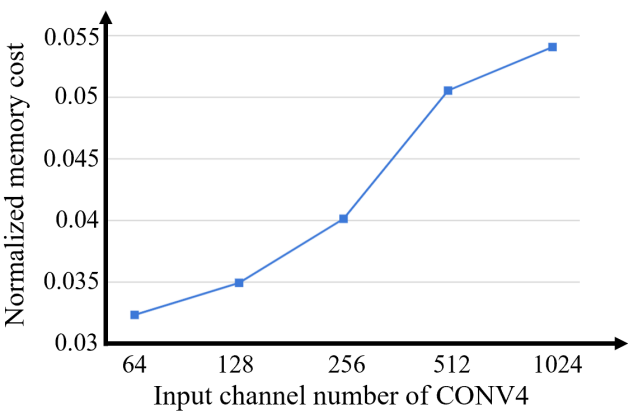
The relationship between the memory saving and the input channel number of the fourth deconvolution layer (CONV4) on the generator is also investigated. Note that increasing the input channel number of the fourth convolution layer (CONV4) will increase its DOR and at the same time the memory cost. On the other hand, eventually a high enough DOR (above 1024) will enable the layer to be binarized, leading to memory reduction. This can be seen in Fig. 12, where x-axis is the input channel number of CONV4 and the y-axis is the total memory cost of the generator normalized to the original generator without any binarization. Before the input channel number of CONV4 reaches 1024, only the first three deconvolution layers can be binarized, so increasing DOR will result in the quick growth of memory cost. However, when the input channel number of CONV4 is 1024, all the four deconvolution layers can be binarized, which introduces extra memory saving to alleviate the memory cost increment.

IV-C6 Unbalanced Competition

So far, our discussion has focused on the binarization of the generator in a GAN only, as the discriminator takes the same form as conventional CNNs. However, since competition between generator and discriminator is the key of GANs, would a binarized generator still compete well with a full discriminator?

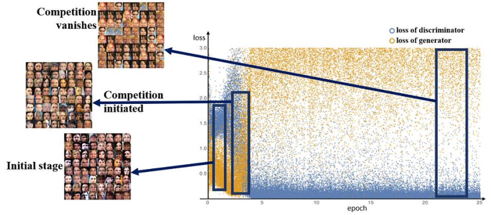
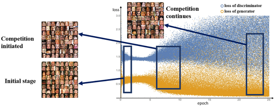
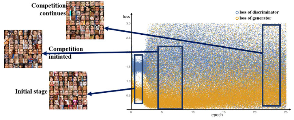
The loss values for the discriminator network and PBGen under Setting F are depicted in Fig. 13, where x-axis indicates the number of epochs and y-axis is the loss value. The images generated from different number of epochs are also exhibited aside. From the figure we can see that during the initial stage, distorted faces are generated. As the competition is initiated, image quality improves. But very quickly, the competition vanishes, and the generated images stop improving. However, when we binarize the discriminator at the same time (Setting H), the competition continues to improve image quality, as can be seen in Fig. 14.

We further plot the loss values of the discriminator and the generator of the original DCGAN (Setting A), and the results are shown in Fig. 15. It is very similar to Fig. 14, except that the competition is initiated earlier, which is due to the stronger representation power of both the generator and the discriminator before binarization. These figures confirm that the quick disappearance of competition is mainly due to the unbalanced generator and discriminator, which should be avoided.

Figure 13: Loss values of the original discriminator and PBGen under Setting F along epochs

Figure 14: Loss values of binarized discriminator and PBGen under Setting H along epochs

Figure 15: Loss values of the discriminator and the generator in original DCGAN under Setting A along epochs

V Conclusion

We now explore the quality of the images generated from balanced competition using Setting H. The images generated are shown in Fig. 5h and Fig. 10h, the quality of which is apparently better than the rest in Fig. 5 and Fig. 10 respectively. To further confirm this quantitatively, we compute the average SWD values of those images, which is 0.034 in average. This is even smaller than any average SWD values listed in TABLE III, which shows that the images are of better quality, even compared with the original DCGAN.

Figure 16: SWD v.s. resolutions under all different settings

V-1 Summary

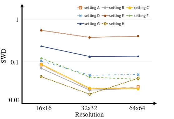
To summarize the discussion and comparisons in this section, we plot the SWD v.s. resolution curves for all the 8 settings in Fig. 16. It allows a complete view of how these different settings compare in terms of similarity as a whole and fine details. From the figure we can see that Setting H gives the best similarity as a whole, while Setting C yields the finest detailed attributes.

Consequently, utilizing the degree of redundancy as a tool, we can efficiently find out eligible layers that can be binarized and based on their superposition, a final binarization strategy can be decided. It cannot guarantee an optimal result but does decrease the search space for the final solution from $O(2^{n})$ to $O(n)$ or less, where $n$ is the number of layers, because testing on all combinations of binarization strategy is not necessary and we only need to binarize every single layer with high degree of redundancy to decide the final strategy. Since our theoretical analysis and experiments are based on deconvolutional layers, we believe this method can work for other deconvolution based generators beyond DCGAN.

Compression techniques have been widely studied for convolutional neural networks, but directly adopting them to all layers will fail deconvolution-based generator in generative adversarial networks based on our observation. We propose and validate that the performance of deconvolution-based generator can be preserved when applying binarization to carefully selected layers (PBGen). To accelerate the process deciding whether a layer can be binarized or not, the degree of redundancy is proposed based on theoretical analysis and further verified by experiments. Under the guide of this metric, search space for optimal binarization strategy is decreased from $O(2^{n})$ to $O(n)$ where $n$ is the number of layers in the generator. PBGen for DCGAN can yield up to 25.81$\times$ saving in memory consumption with 1.96$\times$ and 1.32$\times$ speedup in inference and training respectively with little performance loss measured by sliced Wasserstein distance score. Besides, we also demonstrate that both generator and discriminator should be binarized at the same time for a balanced competition and better performance.

Michael Shell Biography text here.

John Doe Biography text here.

Jane Doe Biography text here.

References

- [1] C. Finn, I. Goodfellow, and S. Levine, “Unsupervised learning for physical interaction through video prediction,” in Advances in Neural Information Processing Systems, 2016, pp. 64–72.
- [2] D. Pfau and O. Vinyals, “Connecting generative adversarial networks and actor-critic methods,” arXiv preprint arXiv:1610.01945, 2016.
- [3] T. Salimans, I. Goodfellow, W. Zaremba, V. Cheung, A. Radford, and X. Chen, “Improved techniques for training gans,” in Advances in Neural Information Processing Systems, 2016, pp. 2234–2242.
- [4] I. Goodfellow, “Nips 2016 tutorial: Generative adversarial networks,” arXiv preprint arXiv:1701.00160, 2016.
- [5] C. Ledig, L. Theis, F. Huszár, J. Caballero, A. Cunningham, A. Acosta, A. Aitken, A. Tejani, J. Totz, Z. Wang et al., “Photo-realistic single image super-resolution using a generative adversarial network,” arXiv preprint arXiv:1609.04802, 2016.
- [6] A. Radford, L. Metz, and S. Chintala, “Unsupervised representation learning with deep convolutional generative adversarial networks,” arXiv preprint arXiv:1511.06434, 2015.
- [7] T. Karras, T. Aila, S. Laine, and J. Lehtinen, “Progressive growing of gans for improved quality, stability, and variation,” arXiv preprint arXiv:1710.10196, 2017.
- [8] A. Inc., “Apple Inc. ,” 2017. [Online]. Available: https://www.apple.com
- [9] W. Chen, J. Wilson, S. Tyree, K. Weinberger, and Y. Chen, “Compressing neural networks with the hashing trick,” in International Conference on Machine Learning, 2015, pp. 2285–2294.
- [10] S. Han, H. Mao, and W. J. Dally, “Deep compression: Compressing deep neural networks with pruning, trained quantization and huffman coding,” arXiv preprint arXiv:1510.00149, 2015.
- [11] S. Zhang, Z. Du, L. Zhang, H. Lan, S. Liu, L. Li, Q. Guo, T. Chen, and Y. Chen, “Cambricon-x: An accelerator for sparse neural networks,” in Microarchitecture (MICRO), 2016 49th Annual IEEE/ACM International Symposium on. IEEE, 2016, pp. 1–12.
- [12] K. Guo, L. Sui, J. Qiu, J. Yu, J. Wang, S. Yao, S. Han, Y. Wang, and H. Yang, “Angel-eye: A complete design flow for mapping cnn onto embedded fpga,” IEEE Transactions on Computer-Aided Design of Integrated Circuits and Systems, vol. 37, no. 1, pp. 35–47, 2018.
- [13] C. Wang, L. Gong, Q. Yu, X. Li, Y. Xie, and X. Zhou, “Dlau: A scalable deep learning accelerator unit on fpga,” IEEE Transactions on Computer-Aided Design of Integrated Circuits and Systems, vol. 36, no. 3, pp. 513–517, 2017.
- [14] I. Hubara, M. Courbariaux, D. Soudry, R. El-Yaniv, and Y. Bengio, “Quantized neural networks: Training neural networks with low precision weights and activations,” arXiv preprint arXiv:1609.07061, 2016.
- [15] A. Al Bahou, G. Karunaratne, R. Andri, L. Cavigelli, and L. Benini, “Xnorbin: A 95 top/s/w hardware accelerator for binary convolutional neural networks,” in 2018 IEEE Symposium in Low-Power and High-Speed Chips (COOL CHIPS). IEEE, 2018, pp. 1–3.
- [16] F. Li, B. Zhang, and B. Liu, “Ternary weight networks,” arXiv preprint arXiv:1605.04711, 2016.
- [17] D. Zhang, J. Yang, D. Ye, and G. Hua, “Lq-nets: Learned quantization for highly accurate and compact deep neural networks,” in Proceedings of the European Conference on Computer Vision (ECCV), 2018, pp. 365–382.
- [18] F. Conti, P. D. Schiavone, and L. Benini, “Xnor neural engine: A hardware accelerator ip for 21.6-fj/op binary neural network inference,” IEEE Transactions on Computer-Aided Design of Integrated Circuits and Systems, vol. 37, no. 11, pp. 2940–2951, 2018.
- [19] Y. Ling, K. Zhong, Y. Wu, D. Liu, J. Ren, R. Liu, M. Duan, W. Liu, and L. Liang, “Taijinet: Towards partial binarized convolutional neural network for embedded systems,” in 2018 IEEE Computer Society Annual Symposium on VLSI (ISVLSI). IEEE, 2018, pp. 136–141.
- [20] M. Rastegari, V. Ordonez, J. Redmon, and A. Farhadi, “Xnor-net: Imagenet classification using binary convolutional neural networks,” in European Conference on Computer Vision. Springer, 2016, pp. 525–542.
- [21] S. Han, J. Pool, J. Tran, and W. Dally, “Learning both weights and connections for efficient neural network,” in Advances in Neural Information Processing Systems, 2015, pp. 1135–1143.
- [22] N. P. Jouppi, C. Young, N. Patil, D. Patterson, G. Agrawal, R. Bajwa, S. Bates, S. Bhatia, N. Boden, A. Borchers et al., “In-datacenter performance analysis of a tensor processing unit,” arXiv preprint arXiv:1704.04760, 2017.
- [23] S. Zhou, Y. Wu, Z. Ni, X. Zhou, H. Wen, and Y. Zou, “Dorefa-net: Training low bitwidth convolutional neural networks with low bitwidth gradients,” arXiv preprint arXiv:1606.06160, 2016.
- [24] M. D. Zeiler, D. Krishnan, G. W. Taylor, and R. Fergus, “Deconvolutional networks,” in Computer Vision and Pattern Recognition (CVPR), 2010 IEEE Conference on. IEEE, 2010, pp. 2528–2535.
- [25] M. Jaderberg, A. Vedaldi, and A. Zisserman, “Speeding up convolutional neural networks with low rank expansions,” arXiv preprint arXiv:1405.3866, 2014.
- [26] M. Lin, Q. Chen, and S. Yan, “Network in network,” arXiv preprint arXiv:1312.4400, 2013.
- [27] P. Judd, J. Albericio, T. Hetherington, T. M. Aamodt, and A. Moshovos, “Stripes: Bit-serial deep neural network computing,” in Microarchitecture (MICRO), 2016 49th Annual IEEE/ACM International Symposium on. IEEE, 2016, pp. 1–12.
- [28] D. Miyashita, E. H. Lee, and B. Murmann, “Convolutional neural networks using logarithmic data representation,” arXiv preprint arXiv:1603.01025, 2016.
- [29] X. Xu, Q. Lu, L. Yang, S. Hu, D. Chen, Y. Hu, and Y. Shi, “Quantization of fully convolutional networks for accurate biomedical image segmentation,” in Proceedings of the IEEE Conference on Computer Vision and Pattern Recognition, 2018, pp. 8300–8308.
- [30] C. Zhu, S. Han, H. Mao, and W. J. Dally, “Trained ternary quantization,” arXiv preprint arXiv:1612.01064, 2016.
- [31] A. Zhou, A. Yao, Y. Guo, L. Xu, and Y. Chen, “Incremental network quantization: Towards lossless cnns with low-precision weights,” arXiv preprint arXiv:1702.03044, 2017.
- [32] Z. Cai, X. He, J. Sun, and N. Vasconcelos, “Deep learning with low precision by half-wave gaussian quantization,” arXiv preprint arXiv:1702.00953, 2017.
- [33] M. Courbariaux, Y. Bengio, and J.-P. David, “Binaryconnect: Training deep neural networks with binary weights during propagations,” in Advances in Neural Information Processing Systems, 2015, pp. 3123–3131.
- [34] M. Courbariaux, I. Hubara, D. Soudry, R. El-Yaniv, and Y. Bengio, “Binarized neural networks: Training deep neural networks with weights and activations constrained to+ 1 or-1,” arXiv preprint arXiv:1602.02830, 2016.
- [35] Y. Ding, J. Liu, J. Xiong, and Y. Shi, “On the universal approximability and complexity bounds of quantized relu neural networks,” arXiv preprint arXiv:1802.03646, 2018.
- [36] J. Wang, Q. Lou, X. Zhang, C. Zhu, Y. Lin, and D. Chen, “Design flow of accelerating hybrid extremely low bit-width neural network in embedded fpga,” in 2018 28th International Conference on Field Programmable Logic and Applications (FPL). IEEE, 2018, pp. 163–1636.
- [37] X. Zhu, W. Zhou, and H. Li, “Adaptive layerwise quantization for deep neural network compression,” in 2018 IEEE International Conference on Multimedia and Expo (ICME). IEEE, 2018, pp. 1–6.
- [38] S. Yin, S. Tang, X. Lin, P. Ouyang, F. Tu, L. Liu, and S. Wei, “A high throughput acceleration for hybrid neural networks with efficient resource management on fpga,” IEEE Transactions on Computer-Aided Design of Integrated Circuits and Systems, vol. 38, no. 4, pp. 678–691, 2018.
- [39] L. Zhuang, Y. Xu, B. Ni, and H. Xu, “Flexible network binarization with layer-wise priority,” arXiv preprint arXiv:1709.04344, 2017.
- [40] X. Xu, Q. Lu, T. Wang, Y. Hu, C. Zhuo, J. Liu, and Y. Shi, “Efficient hardware implementation of cellular neural networks with incremental quantization and early exit,” ACM Journal on Emerging Technologies in Computing Systems (JETC), vol. 14, no. 4, p. 48, 2018.
- [41] I. Chakraborty, D. Roy, A. Ankit, and K. Roy, “Efficient hybrid network architectures for extremely quantized neural networks enabling intelligence at the edge,” arXiv preprint arXiv:1902.00460, 2019.
- [42] A. Prabhu, V. Batchu, R. Gajawada, S. A. Munagala, and A. Namboodiri, “Hybrid binary networks: Optimizing for accuracy, efficiency and memory,” in 2018 IEEE Winter Conference on Applications of Computer Vision (WACV). IEEE, 2018, pp. 821–829.
- [43] I. Chakraborty, D. Roy, I. Garg, A. Ankit, and K. Roy, “Pca-driven hybrid network design for enabling intelligence at the edge,” arXiv preprint arXiv:1906.01493, 2019.
- [44] J. Song, “Binary generative adversarial networks for image retrieval,” arXiv preprint arXiv:1708.04150, 2017.
- [45] I. Goodfellow, J. Pouget-Abadie, M. Mirza, B. Xu, D. Warde-Farley, S. Ozair, A. Courville, and Y. Bengio, “Generative adversarial nets,” in Advances in neural information processing systems, 2014, pp. 2672–2680.
- [46] S. Reed, Z. Akata, X. Yan, L. Logeswaran, B. Schiele, and H. Lee, “Generative adversarial text to image synthesis,” arXiv preprint arXiv:1605.05396, 2016.
- [47] X. Chen, Y. Duan, R. Houthooft, J. Schulman, I. Sutskever, and P. Abbeel, “Infogan: Interpretable representation learning by information maximizing generative adversarial nets,” in Advances in Neural Information Processing Systems, 2016, pp. 2172–2180.
- [48] M. Arjovsky, S. Chintala, and L. Bottou, “Wasserstein generative adversarial networks,” in International Conference on Machine Learning, 2017, pp. 214–223.
- [49] X. Mao, Q. Li, H. Xie, R. Y. Lau, Z. Wang, and S. P. Smolley, “Least squares generative adversarial networks,” arXiv preprint ArXiv:1611.04076, 2016.
- [50] cs231n Course Materials, “Implementation as Matrix Multiplication,” 2017. [Online]. Available: http://cs231n.github.io/convolutional-networks/#layers
- [51] F. N. Iandola, S. Han, M. W. Moskewicz, K. Ashraf, W. J. Dally, and K. Keutzer, “Squeezenet: Alexnet-level accuracy with 50x fewer parameters and¡ 0.5 mb model size,” arXiv preprint arXiv:1602.07360, 2016.
- [52] M. Abadi, A. Agarwal, P. Barham, E. Brevdo, Z. Chen, C. Citro, G. S. Corrado, A. Davis, J. Dean, M. Devin et al., “Tensorflow: Large-scale machine learning on heterogeneous distributed systems,” arXiv preprint arXiv:1603.04467, 2016.
- [53] T. Kim, “DCGAN-tensorflow,” 2017. [Online]. Available: https://github.com/carpedm20/DCGAN-tensorflow
- [54] Z. Liu, P. Luo, X. Wang, and X. Tang, “Deep learning face attributes in the wild,” in Proceedings of International Conference on Computer Vision (ICCV), 2015.
- [55] J. Cha, “tf.gans-comparision,” 2017. [Online]. Available: https://github.com/qingshan412/tf.gans-comparison
- [56] L. Theis, A. van den Oord, and M. Bethge, “Anote on the evaluation of generative models,” stat, vol. 1050, p. 24, 2016.
- [57] Y. Wu, Y. Burda, R. Salakhutdinov, and R. Grosse, “On the quantitative analysis of decoder-based generative models,” arXiv preprint arXiv:1611.04273, 2016.
- [58] A. Odena, C. Olah, and J. Shlens, “Conditional image synthesis with auxiliary classifier gans,” arXiv preprint arXiv:1610.09585, 2016.