OGLE-2017-BLG-1130: THE FIRST BINARY GRAVITATIONAL MICROLENS DETECTED FROM Spitzer ONLY

Abstract

We analyze the binary gravitational microlensing event OGLE-2017-BLG-1130 (mass ratio $q\sim 0.45$), the first published case in which the binary anomaly was only detected by the Spitzer Space Telescope. This event provides strong evidence that some binary signals can be missed by observations from the ground alone but detected by Spitzer. We therefore invert the normal procedure, first finding the lens parameters by fitting the space-based data and then measuring the microlensing parallax using ground-based observations. We also show that the normal four-fold space-based degeneracy in the single-lens case can become a weak eight-fold degeneracy in binary-lens events. Although this degeneracy is resolved in event OGLE-2017-BLG-1130, it might persist in other events.

P. Mróz

1 Introduction

The projected Einstein radii, $\tilde{r}_{\rm E}\equiv{\rm AU}/\pi_{\rm E}$, of typical Galactic gravitational microlensing events are of the order of a few astronomical units (au). Hence, the relative lens-source positions seen from the ground and from a satellite in solar orbit appear to be different. This results in different light curves, and a combined analysis of the light curves should lead to the measurement of the microlens-parallax vector $\pi_{\rm E}$ (Refsdal, 1966; Gould, 1994), which is related to the physical lens parameters by

$$\mbox{\boldmath$\pi_{\rm E}$}\equiv\frac{\pi_{\rm rel}}{\theta_{\rm E}}\frac{\mbox{\boldmath$\mu$}}{\mu};\quad\theta_{\rm E}\equiv\sqrt{\kappa M\pi_{\rm rel}}$$ (1)

where $(\pi_{\rm rel},\mbox{\boldmath$\mu$})$ are the lens-source relative (parallax, proper motion), $\theta_{E}$ is the angular Einstein radius, $\kappa\equiv 4G/(c^{2}{\rm au})\simeq 8.14\ {\rm mas}/M_{\odot}$. The measurement of $\pi_{\rm E}$ is important because, by itself, it strongly constrains the lens mass $M$ and distance $D_{L}$ (Han & Gould, 1995), and provided that $\theta_{\rm E}$ is also determined, enables one to measure both quantities,

$$M=\frac{\theta_{E}}{\kappa\pi_{\rm E}};\quad D_{L}=\frac{\rm AU}{\pi_{\rm E}\theta_{E}+\pi_{S}},$$ (2)

where $\pi_{S}={\rm AU}/D_{S}$ is the parallax of the lensed star (source), and $D_{S}$ is the distance to the source

Since 2014, Spitzer Space Telescope has measured the microlens parallax $\pi_{\rm E}$ for hundreds of microlensing (single and binary) events, proving it to be an excellent microlensing parallax measurement satellite (Dong et al., 2007; Udalski et al., 2015; Yee et al, 2015a; Zhu et al., 2015; Calchi Novati et al., 2015). However, the usefulness of Spitzer observations in characterizing binaries can extend beyond measuring parallax. For example, in the case of event OGLE-2014-BLG-0124 (Udalski et al., 2015), the planetary signal was independently detected from Spitzer.

For most binary microlensing events, the caustic structures and lens parameters can be directly determined by ground-based observations. In such cases, Spitzer data are only used to measure the satellite parallax and sometimes to resolve the remaining degeneracies. Nevertheless, it is possible, in principle, that the binary signal would be detected solely from the satellite, in which case the ground-based data would be used to measure the parallax parameters. This happens in the binary event OGLE-2017-BLG-1130, for which the ground-based data show no deviation from a single-lens light curve.

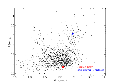
Figure 4: OGLE-IV color magnitude diagram of the stars (black dots) within $2^{\prime}\times 2^{\prime}$ of OGLE-2017-BLG-1130. The red and blue dots show the source star and the centroid of the red clump stars, respectively.

Light curves of single-mass lensing events obtained from ground-based observatories and one space-based observatory typically yield a set of four degenerate solutions (Refsdal, 1966; Gould, 1994; Gould & Horne, 2013; Calchi Novati et al., 2015; Yee et al., 2015), which are often denoted as (+,+), ($-$,$-$), (+,$-$), and ($-$,+). Here the first and second signs in each parenthesis represent the signs of the lens-source impact parameters as seen from Earth and from the satellite, respectively. See Figure 4 of Gould (2004) for the sign conventions. This four-fold degeneracy can be expressed as (+,$-$)$\times$(same, opposite), where the signs in the first parenthesis represent the signs of the impact parameter seen from Earth, and same (or opposite) means that the source trajectories seen from Earth and from the satellite pass on the same side (or opposite sides) with respect to the lens.

For binary-lens events that are well covered by the observations, the (same, opposite) degeneracy is generally broken due to the asymmetry in the light curve. If the degeneracy remains unresolved, we usually consider that “opposite side of the lens” means “opposite side of the nearby component of lens primary”, as has been seen in previous cases (Zhu et al., 2015; Han et al., 2016). For binary-lens events that are not well covered, such as the present event OGLE-2017-BLG-1130, the source trajectories seen from Earth and the satellite in the “opposite” solution can in principle pass on the opposite side of either the whole lens system or of the nearby component (see Section 3.3.1), and there can be as many as eight degenerate solutions. We identify this new form of the four-fold degeneracy here for the first time. We show that while it is resolved for OGLE-2017-BLG-1130, it may persist in the case of other events.

In this paper, we present the analysis of the Spitzer binary event OGLE-2017-BLG-1130. This is the first published case in which the binary anomaly is detected by Spitzer only. We summarize the ground-based and space-based observations in Section 2, describe the light curve modeling in Section 3, and derive the physical properties of the binary system in Section 4. In Section 5, we discuss the potentially new form of the four-fold degeneracy that occurs in this event.

2 Observations

2.1 Ground-Based Alert and Follow-up

At UT 11:57 of 2017 June 19 (HJD^′ = HJD$-$2450000 = 7924.00), the OGLE collaboration identified the microlensing event OGLE-2017-BLG-1130 at equatorial coordinates (R.A., decl.)₂₀₀₀ = ($18^{\rm h}01^{\rm m}36\fs 93$, $-27\arcdeg 39\arcmin 56\farcs 9$) with corresponding Galactic coordinates $(l,b)$ = (2.88^∘, $-$2.39^∘), based on observations with the 1.3m Warsaw telescope with 1.4 deg² camera at Las Campanas in Chile. This microlensing event, lies in the OGLE-IV field BLG511, which was covered with a cadence of $1\,{\rm hr^{-1}}$ (Udalski et al., 1994; Udalski, 2003; Udalski et al., 2015).

The Korea Microlesning Telescope Network (KMTNet, Kim et al. 2016) observed this event from its three 1.6m telescopes at CTIO (Chile, KMTC), SAAO (South Africa, KMTS) and SSO (Australia, KMTA), in its BLG03 field, with cadence of $2\,{\rm hr^{-1}}$. KMTNet designated the event as BLG03K0102.032555.

All ground-based data were reduced using variants of the image subtraction method (Alard & Lupton, 1998; Woźniak, 2000; Albrow et al., 2009).

Both OGLE and KMTNet data were adversely affected by a diffraction spike from a nearby bright star. Because this star was very blue, the $V$-band light curves from both surveys were completely corrupted. Since these would normally be used to determine the source color $(V-I)_{S}$, we had to develop a novel technique to measure this quantity, a point to which we return below.

The $I$-band light curves also suffered from some degradation depending on the observatories (OGLE, KMTS, KMTC, KMTA) where the data were taken. Because the ground-based data are well-characterized by a Paczyński (1986) “point lens” fit, we could afford to be quite conservative in including in the modeling only the best ground-based data. We found that the OGLE and KMTS data were of comparable, and generally quite good, quality. On the other hand, the KMTC and KMTA data showed much larger scatter and also much greater systematics. We therefore do not use KMTC and KMTA data in our analysis. Closer investigations of the OGLE and KMTS data revealed that both display some systematics in “better seeing” images. This is not surprising because diffraction spikes are more pronounced in better seeing. Although these effects were not severe, to be conservative, we nevertheless eliminated all OGLE images with FWHM$<1.17^{\prime\prime}$ (4.5 pixels) and all KMTS images with FWHM$<2.08^{\prime\prime}$ (5.2 pixels).

2.2 Spitzer Follow-up

OGLE-2017-BLG-1130 was originally selected as a Spitzer target within the framework of the protocols of Yee et al. (2015b). These protocols are designed to obtain an “objective sample” to measure the Galactic distribution of planets despite the fact that humans must make observing decisions based on real-time data. Very briefly, events can be selected “objectively”, “subjectively”, or “secretly”. Events that meet certain objective criteria must be observed according to the pre-specified rules. As a consequence, all planets found in the data enter into the Galactic-distribution sample. Events can be selected subjectively by the Spitzer team for any reason. However, only planets that do not give rise to significant signal in the data available at the time of the announcement can be included in the Galactic-distribution sample. The announcement must specify the candence of observations and the time (or conditions) under which the observations will cease. Finally, events can be selected “secretly”, i.e., without public announcement. In this case Spitzer observations are commenced with no specifications on when they might terminate. Such events may be converted by the team from “secret” to “subjective” by making a public announcement. In this case, planets can enter the Galactic-sample according to the conditions governing “subjective” events, and in particular, according to the date of the public announcement.

OGLE-2017-BLG-1130 was initially chosen “secretly” on June 19, just a few hours after it was announced by OGLE (and just before the Spitzer upload time) because it was judged by the upload subteam that it might reach relatively high magnification based on the data then available. In particular, this subteam does not generally have the authority to choose events subjectively without consulting the team, other than in exceptional circumstances. The following week, the event’s future course remained too uncertain to decide between stopping observations and choosing it subjectively. Hence, it remained “secret”. Finally, at UT 16:56 on July 2, shortly before the third upload, it was publicly announced as “subjective”. Observations continued until the end of the Spitzer window. The binary signal in the Spitzer data only became discernible at UT 00:28 on August 9, i.e., five days after the final observation, when the reduced Spitzer data were circulated to the team. It was specifically noted by SCN about 16 hours later. Because OGLE-2017-BLG-1130L is not planetary, these details do not directly impact any scientific conclusion. However, we document them here nonetheless in order to maintain homogeneous records for planets and binaries.

3 Light Curve Modeling

3.1 Initial Solution Search

We fit a binary microlensing model to the light curve to explain the observed variation in brightness. The standard binary modeling needs seven basic parameters: the time of the source closest approach to the center of mass of the lens system, $t_{0}$; the impact parameter with respect to the center of mass of the lens system normalized by the Einstein radius, $u_{0}$; the Einstein radius crossing time, $t_{\rm E}\equiv\theta_{\rm E}/\mu$, where $\mu$ is the relative lens-source proper motion; the source radius normalized by the Einstein radius, $\rho\equiv\theta_{\star}/\theta_{\rm E}$; the projected separation of the binary components normalized to the Einstein radius, $s$; the binary mass ratio, $q$; and the angle between the binary-lens axis and the lens-source relative motion, $\alpha$. With these seven parameters, we can calculate the binary magnification as a function of time $A(t)$. To describe the blend in the crowded stellar fields, we further introduce two flux parameters, the source flux $(F_{\rm S,j})$ and the blending flux $(F_{\rm B,j})$ so that the observed flux at given time $t_{i}$ is

$$F_{\rm j}(t_{i})=F_{\rm S,j}\cdot A(t_{i})+F_{\rm B,j}\ .$$ (3)

where $A(t_{i})$ is the magnification at $t_{i}$. These flux parameters are found for each data set and each trial of geometric parameters from a linear fit.

We calculate the binary lens magnification $A(t)$ using the advanced contour integration code, VBBinaryLensing . This code includes a parabolic correction in Green’s line integral that automatically adjusts the step size of integration based on the distance to the binary caustic, in order to achieve a desired precision in magnification. See Bozza (2010) for more details.

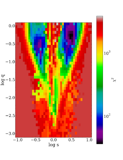
Figure 1: $\chi^{2}$ results of the grid search projected onto the ($\log s$, $\log q$) plane.

To find the best-fit model, we first fit the Spitzer data only, since the binary signal is not detected from ground. We conducted a grid in the ($\log s$, $\log q$, $\alpha$) parameter space, with 40 values equally spaced between $-1\leq$ $\log s$ $\leq 1$, $-3\leq$ $\log q$ $\leq 0$ and $0^{\circ}$$\leq\alpha\leq 360^{\circ}$, respectively. For each set of ($\log s$, $\log q$, $\alpha$), we find the minimum $\chi^{2}$ by using a function based on the Nelder-Mead simplex algorithm from the SciPy package on the remaining parameters ($t_{0}$, $u_{0}$, $t_{E}$, log $\rho$). We find the global minimum at $\log s\sim 0.5$, $\log q\sim-0.3$ and $\alpha\sim 108^{\circ}$, and the result of the grid search clearly shows the close-wide degeneracy (See Figure 1). Other local minima will be discussed in Section 3.3.

We then perform a Markov Chain Monte Carlo (MCMC) analysis on all parameters around the initial solutions found by the previous grid search, which employs the emcee ensemble sampler (Foreman-Mackey et al., 2013).

3.2 Inclusion of the Microlensing Parallax Effect

The microlensing parallax effect must be taken into account in order to simultaneously model the ground-based and space-based data. This effect invokes two additional parameters, $\pi_{\rm E,N}$ and $\pi_{\rm E,E}$, which are the northern and eastern components of the microlens parallax vector $\pi_{{\rm E}}$. We extract the geocentric locations of Spitzer during the entire season from the JPL Horizons website and project them onto the observer plane. The projected locations are then oriented and rescaled according to a given $\pi_{\rm E}$ to determine the lens-source vector as seen from Spitzer.

As described in Section 1, the normal four-fold space-based degeneracy (Refsdal, 1966; Gould, 1994) for single lens events $[(+,+),(-,-),(+,-),(-,+)]$ is potentially ambiguous when applied to binary events. That is, for single-lens events, this degeneracy can be expressed as $(+,-)\times$(same, opposite), where “same” and “opposite” refer to the location of the source trajectory as seen from the satellite relative to the location as seen from Earth. However, for a wide binary lens, this degeneracy can become six fold: $(+,-)\times$(same, opposite nearby component, opposite whole binary). In some cases, the “opposite nearby component” will become two-fold degenerate with the trajectory closer to the primary star or to the secondary star (See Section 3.3.1). Therefore, in the most general case, there would be eight degenerate solutions. This form of degeneracy was not previously anticipated and appears for the case of OGLE-2017-BLG-1130 for the first time. The parameters of these solutions are shown in Table 1.

3.3 Summary of Local Minima

For completeness, we present all local minima in this section. These minima can all explain the data qualitatively. As we subsequently show, however, only the pair of $(+,-)\times$(same) solutions, i.e., the $(+,+)$ and $(-,-)$ solutions, are viable.

3.3.1 Best-fit Model

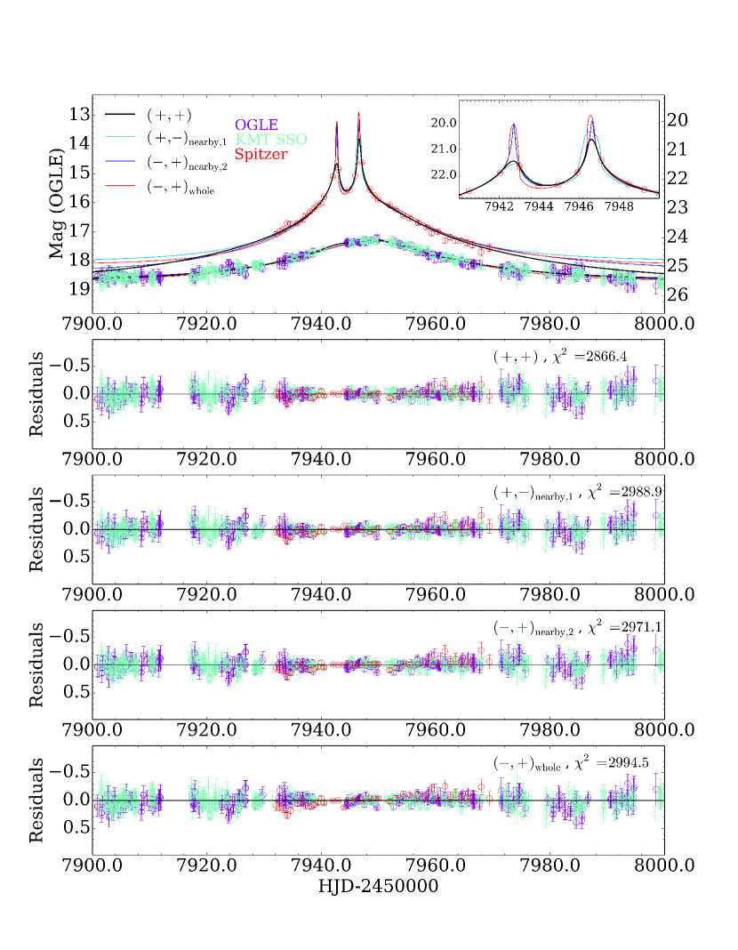
Figure 2: Light curves of the best-fit model and its degenerate counterparts.

The best-fit models are the (+,+) and ($-$,$-$) solutions listed in Table 1. After finding these two solutions, we looked for large-parallax degenerate solutions by setting the initial guess of parallax parameters to large values and running a longer MCMC. The other four-fold degenerate solutions are all found by this method. As discussed above, the source trajectories seen from Earth and the satellite in the“opposite” solution could pass on either the opposite side of the whole lens system (two solutions) or of the nearby component (four solutions). Therefore, there are six possible large-parallax degenerate solutions. We present the light curves and caustic plots for the (+, +), (+,$-$)${}_{\text{nearby,1}}$, ($-$,+)${}_{\text{nearby,2}}$ and ($-$, +)_whole in Figures 2 and 3. The solutions of $u_{0}\pm$ degeneracy are similar to each other (the caustics are almost the same, with trajectories reflected about the $x$-axis), and we only present figures for one solution for each pair. Moreover, in event OGLE-2017-BLG-1130, the binary signal is only detected by Spitzer, and it is easier to see the difference between different solutions if the source trajectories seen by Spitzer are fixed on the caustics plots. Therefore, we choose to present figures of solutions with the same sign of $u_{0}$ as seen from Spitzer (and different signs of $u_{0}$ as seen from Earth).

The three pairs of large-parallax solutions represented in the three diagrams [(+,$-$)_nearby,1, ($-$,+)_nearby,2 and ($-$,+)_whole] can qualitatively explain the data, but they are actually not viable. In addition to their larger $\chi^{2}$, these solutions all have excessive negative blending. The $F_{S}$ parameters measured from the OGLE data set are too large, implying that the unmagnified source fluxes, $I_{S,\rm OGLE}=18-2.5\log_{10}(F_{S,{\rm OGLE}})<17.3$, are clearly ruled out by the total baseline of OGLE data, $I_{\rm s,OGLE}=18.69$.

3.3.2 Close/Wide degeneracy

Here we consider the “close-wide” degeneracy. The best-fit model listed in Section 3.3.1 is the “wide” ($s>$1) solution, and we discuss the “close” ($s<$1) solution here. In this case, the four-fold degeneracy is reduced into the two-fold $u_{0}\pm$ degeneracy. First, for a close lens there is only one diamond-shaped caustic so there are only two large-parallax solutions. Second, the large-parallax solutions are disfavored by $\Delta\chi^{2}>100$. Their parameters are shown in Table 2. These two solutions have $\chi^{2}$ larger than the best-fit model by about 70 and hence are rejected.

3.3.3 Other solutions

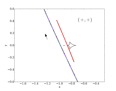
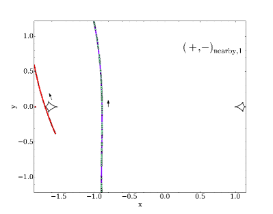
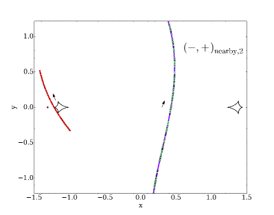
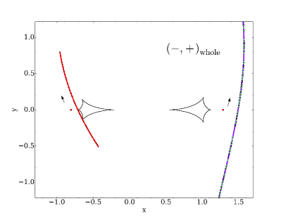
Figure 3: Caustics and trajectories of the best-fit model and its degenerate solutions. The red (blue) curve shows the source trajectory as seen from Spitzer (Earth). The red dots mark the positions of the lens components.

It is possible to reproduce the two peaks in light curves seen in Spitzer data provided that the trajectories seen by Spitzer pass the diamond-shaped caustics at different angles while the other parameters remain approximately the same. For example, a source trajectory at roughly 90 degrees to the one shown in Figure 3 would pass the bottom cusp and then the right-most cusp, producing two bumps as seen in the light curve. There are two such solutions, one corresponding to the best-fit model and the other corresponding to the “close” solution. These two solutions have $\chi^{2}$ larger than the best-fit model by more than 130 and hence are rejected.

We have also tried binary-source models. These fail by $\Delta\chi^{2}\sim 300$ for Spitzer only and by $\Delta\chi^{2}\sim 310$ for combined data sets, so they are not considered.

4 Physical Parameters

The amplitude of the parallax vector, $\pi_{\rm E}=0.097\pm 0.005,$ is well-measured. Hence, if the Einstein radius $\theta_{\rm E}$ were also well measured, we could directly determine the lens mass $M=\theta_{\rm E}/\kappa\pi_{\rm E}$ and lens-source relative parallax, $\pi_{\rm rel}=\theta_{\rm E}\pi_{\rm E}$. Unfortunately, as is apparent from Table 1, the normalized source size, $\rho=\theta_{\star}/\theta_{\rm E}$, is barely detected. In fact, as we show below, $\rho$ is consistent with zero at the $\Delta\chi^{2}=1.5$ level. The fact that $\rho$ is weakly constrained implies that $\theta_{\rm E}=\theta_{\star}/\rho$ is likewise weakly constrained. We will therefore ultimately require a Bayesian analysis to estimate the mass and distance of the lens system.

Even though $\rho$ is not strongly constrained, we must still measure $\theta_{\star}$ in order to make use of it at all. This turns out to require a somewhat novel technique.

4.1 Measurement of $\theta_{\star}$

The usual path to measuring $\theta_{\star}$ (Yoo et al., 2004) is to start by measuring the source color and magnitude on an instrumental color-magnitude diagram, usually $(V-I,I)_{S}$, and to find the offset of this quantity from the clump, i.e., $\Delta(V-I,I)=(V-I,I)_{S}-(V-I,I)_{\rm cl}$. Then one determines the intrinsic position of the clump $(V-I,I)_{\rm cl,0}=(1.06,14.35)$ from the literature (Nataf et al., 2013; Bensby et al., 2013), and so $(V-I,I)_{S,0}=(V-I,I)_{\rm cl,0}+\Delta(V-I,I)$. Finally, one transforms from $V/I$ to $V/K$ using the color-color relations of Bessell & Brett (1988) and then applies the color/surface-brightness relations of Kervella et al. (2004).

In our case, unfortunately, we cannot measure $V_{S}$ because the $V$-band images from both OGLE and KMTNet are corrupted by diffraction spikes from a nearby bright, blue star. Moreover, a frequently used back-up (for cases that $V$-band data are too poor to be used), namely an $H$-band light curve, is also not available in the present case.

We therefore introduce a novel approach to this problem by employing the Spitzer $3.6\,\mu$m (“$L$-band”) observations to determine the $(V-I)$ color. In fact, there is a well-developed technology for contructing $VIL$ color-color relations for Spitzer microlensing data (Calchi Novati et al., 2015). Normally, this is used when the Spitzer source flux is not well constrained by the microlensing light curve, which often occurs if the Spitzer data begin well after the peak. In these cases, the well-measured $(V-I)_{S}$ color is then used to determine $(I-L)_{S}$ and thereby strongly constrain the Spitzer source flux (and therefore the magnification changes as a function of time).

In the present case, we invert this procedure. From the measured $(I-L)_{S}=1.48\pm 0.15$ [or $(I-L)_{S}=1.44\pm 0.15$] color derived from the fits in Table 1, we find $(V-I)_{S,\rm OGLE}=2.10\pm 0.15$ [or $(V-I)_{S,\rm OGLE}=2.07\pm 0.15$]. See Figure 4. Then, applying all the steps above, we find

$$\begin{split}\theta_{\star}&=0.92\pm 0.10~{}\mu{\rm\,as}\quad{\rm for~{}(+,+)~{}solution},\\ \theta_{\star}&=0.90\pm 0.10~{}\mu{\rm\,as}\quad{\rm for~{}(-,-)~{}solution}.\end{split}$$ (4)

4.2 Bayesian Analysis

We begin our Bayesian analysis by extracting from the MCMC the best fit $a_{0,i}$ and covariance $c_{ij}$ of the three measured quantities $a_{i}=(\tilde{v}_{\rm l,hel},\tilde{v}_{\rm b,hel},t_{\rm E,hel})$. Here,

$$\mbox{\boldmath$\tilde{v}$}_{\rm hel}=\mbox{\boldmath$\tilde{v}$}_{\rm geo}+\mbox{\boldmath$v$}_{\oplus,\perp};\qquad t_{\rm E,hel}=\frac{{\tilde{v}}_{\rm geo}}{{\tilde{v}}_{\rm hel}}t_{\rm E}$$ (5)

are the helicentric velocity and timescale, where $v_{\oplus,\perp}(\rm N,E)=(-0.73,27.22){\rm km}\,{\rm s}^{-1}$, which is equivalent to $v_{\oplus,\perp}(\rm l,b)=(12.98,-23.94){\rm km}\,{\rm s}^{-1}$.

We consider bulge sources and disk or bulge lenses drawn randomly from the Galactic model in Zhu et al. (2017a), and for each trial we draw a mass of the primary star randomly from a Kroupa (2001) mass function. We then calculate the resulting $\theta_{\rm E}=\sqrt{\kappa M\pi_{\rm rel}}$, ${\mbox{\boldmath$\tilde{v}$}}_{\rm hel}={\mbox{\boldmath$\mu$}}_{\rm hel}{\rm AU}/\pi_{\rm rel}$, $t_{\rm E,hel}=\theta_{E}/\mu_{\rm hel}$ and $\rho=\theta_{\star}/\theta_{E}$.

We then evaluate

$$\begin{split}\chi^{2}_{\rm gal}&=\chi^{2}(\rho)+\chi^{2}_{\rm dyn},\\ \chi^{2}_{\rm dyn}&=\sum_{i,j=1}^{3}(a-a_{0})_{i}b_{ij}(a-a_{0})_{j},\end{split}$$ (6)

where $a_{i}=(\tilde{v}_{\rm l,hel},\tilde{v}_{\rm b,hel},t_{\rm E,hel})$, $b\equiv c^{-1}$, and $\chi^{2}(\rho)$ represents the lower envelope of the $(\chi^{2}\ \rm vs.\ \rho)$ diagram derived from the MCMC (Calchi Novati et al., 2018). We then weight all trials by the probability evaluated by combining $\chi^{2}_{\rm gal}$ and the microlensing rate contribution,

$$w_{i}=\exp(-\chi^{2}_{\rm gal,i}/2)\times\theta_{\rm E,i}\mu_{\rm i}.$$ (7)

We also take into account the flux constraint on the lens. The blend flux is $I_{b}=19.9$ and $I_{b}=20.0$ for the $(+,+)$ and $(-,-)$ solutions. We find that the microlensed source is displaced from the “baseline object” by $0.22^{\prime\prime}\pm 0.02^{\prime\prime}$. This implies that no more than about 50% of the blended light could be due to the lens. To be conservative, we set an upper limit of 75%, which implies $I_{l}>20.2$ and $I_{l}>20.3$ in the two cases. We then use these as the upper limits on the lens flux. We adopt the mass-luminosity relation

$$M_{I}=4.4-8.5\log\biggl{(}\frac{M_{\rm prim}}{M_{\odot}}\biggr{)},$$ (8)

where $M_{I}$ is the absolute magnitude in $I$-band and $M_{\rm prim}$ is the mass of the primary. Then the lens distance should satisfy

$$M_{I}+5\log\biggl{(}\frac{D_{L}}{10{\ \rm pc}}\biggr{)}+A_{I}\geq I_{b},$$ (9)

where $D_{L}$ is the distance to the lens and the extinction $A_{I}=I_{\rm RC}-I_{\rm RC,0}=1.52$. We reject trials that violate this relation.

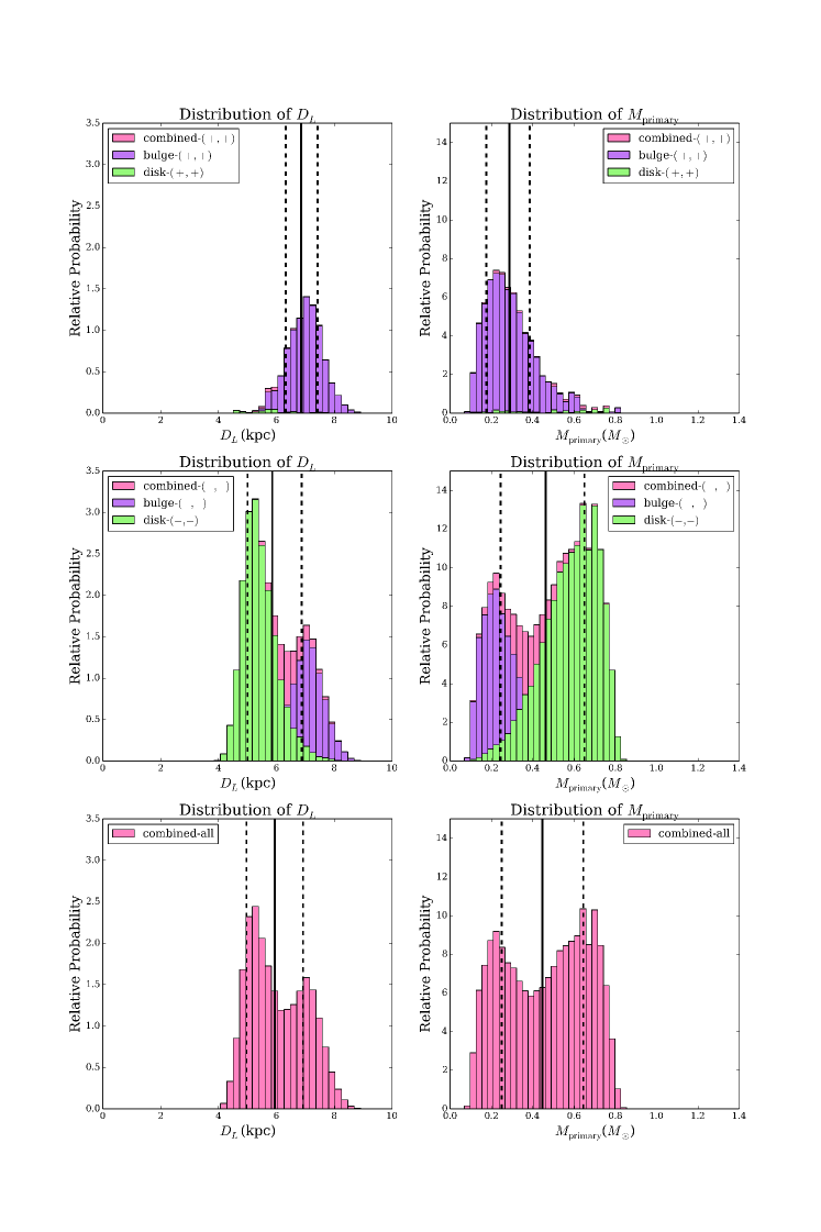
Figure 5: Distribution of $D_{L}$ and $M_{\rm prim}$ from the Bayesian analysis. Top: the $(+,+)$ solution. Middle: the $(-,-)$ solution. Bottom: combined distributions. The distributions are arbitrarily normalized.

The results of the Bayesian analysis are shown in Figure 5. For bulge lenses, the $(+,+)$ and $(-,-)$ solutions yield similar distributions of physical parameters. On the other hand, for disk lenses, the $(-,-)$ solution is strongly favored because its direction is right in the direction of Galactic rotation. The ratio between the probability of bulge and disk lenses in the $(-,-)$ solution is about 1/2.2, while the disk lens part of the $(+,+)$ solution is almost ruled out. In principle, the two solutions $(+,+)$ and $(-,-)$ should be weighted by $e^{-\chi^{2}/2}$. However, the difference in $\chi^{2}$ is well-within the margin of what can be produced by typical microlensing systematics. Hence, we just weight them by total probability and so obtain $M_{\rm prim}=0.45\pm 0.20M_{\odot}$ and $D_{L}=5.9\pm 1.0\,{\rm kpc}$.

4.3 Future Resolution

From

$$M=\frac{\mu_{\rm hel}t_{{\rm E},{\rm hel}}}{\kappa\pi_{\rm E}}$$ (10)

and

$$\pi_{\rm rel}=\pi_{\rm E}\mu_{\rm hel}t_{{\rm E},{\rm hel}},$$ (11)

we can measure the lens mass and lens-source relative parallax if a future determination of the lens-source relative heliocentric proper motion $\mbox{\boldmath$\mu$}_{\rm hel}$ is available. Because the errors in $\pi_{\rm E}$ and $t_{\rm E}$ are about 10% and 5%, the mass and relative parallax can ultimately be constrained to $\pm 15\%$, provided that the proper-motion measurement is more precise than this.

The vector proper motion measurement would also decisively rule out (or possibly confirm one of) the other solutions that we analyzed in Section 3.3. As discussed above, the larger parallax solutions are extremely unlikely to be correct due to their large $\chi^{2}$ and excessive negative blending. The proper motion measurement can confirm this conclusion.

To assess when such a measurement can first be made, we first estimate the expected proper motion as a function of the lens mass $M=(1+q)M_{\rm prim}$ and quantities that are directly measured from the light curve

$$\begin{split}{\mbox{\boldmath$\mu$}}_{\rm hel}&={\pi_{\rm rel}\over{\rm AU}}\mbox{\boldmath$\tilde{v}$}_{\rm hel}\\ &={\kappa\pi_{\rm E}^{2}M\over{\rm AU}}(\mbox{\boldmath$\tilde{v}$}_{\rm geo}+\mbox{\boldmath$v$}_{\oplus,\perp})\\ &=\kappa M\biggl{(}{{\mbox{\boldmath$\pi$}}_{\rm E}\over t_{\rm E}}+{\pi_{\rm E}^{2}\over{\rm AU}}\mbox{\boldmath$v$}_{\oplus,\perp}\biggr{)}\end{split}$$ (12)

For the two cases, this yields

$$\begin{split}{\mbox{\boldmath$\mu$}}_{{\rm hel}_{+,+}}(\rm N,E)&=(-4.7,+3.5){\rm mas}\,{\rm yr}^{-1}\biggl{(}{M\over M_{\odot}}\biggr{)};\\ {\mbox{\boldmath$\mu$}}_{{\rm hel}_{-,-}}(\rm N,E)&=(+5.2,+2.9){\rm mas}\,{\rm yr}^{-1}\biggl{(}\frac{M}{M_{\odot}}\biggr{)},\end{split}$$ (13)

i.e., similar amplitudes $\mu_{\rm hel}\simeq 5.9\,{\rm mas}\,{\rm yr}^{-1}(M/M_{\odot})$.

Based on the experience of Batista et al. (2015), who resolved the equally-bright source and lens of OGLE-2005-BLG-169 at a separation of $\sim 60~{}$mas, we can see that such a measurement using present-day instrumentation would require a 15 year wait for an $M\sim 0.7\,M_{\odot}$ ($M_{\rm prim}\sim 0.48\,M_{\odot}$) lens. From Figure 5 and Equation 13, this would imply only a 50% probability of separately resolving the source and lens. However, by this time it is very likely that next generation (“30 meter”) telescopes with adaptive optics will be operating. Since these will have roughly three times better resolution than the current 8-10m telescopes, the lens and source can almost certainly be resolved at first light of these instruments.

5 Discussion

We analyzed the binary-lensing event OGLE-2017-BLG-1130 in which the binary anomaly was only detected by the Spitzer Space Telescope. We found the lens parameters by fitting the space-based data, and we measured the microlensing parallax using ground-based observations.

This event provides strong evidence that some binary signals (as predicted by Mao & Paczynski 1991) can be missed by observations from the ground alone but detected by Spitzer, especially for wide and close binaries. Although space-based data are normally used to measure the microlensing parallax, it is possible that some interesting signals, for example, planetary signals, can only be seen from Spitzer. In event OGLE-2014-BLG-0124, the planetary signal was independently detected from Spitzer, and if the trajectories had been slightly different, the planetary signal could have been detected by Spitzer and missed from the ground. In addition, such binaries may affect the observed event timescale distributions (Wegg et al., 2017; Mróz et al., 2017), as in event OGLE-2017-BLG-1130 the timescale fitted from ground data is about 10 days shorter than the real case. Therefore, the role that Spitzer plays in microlensing observations is more than functioning as a parallax satellite, and it will produce more results of scientific interest in the future.

The binary-lensing event OGLE-2017-BLG-1130 is peculiar in another aspect. We show that the normal four-fold space-based degeneracy can in principle become eight-fold: $(+,-)\times$(same, opposite nearby component & close to primary, opposite nearby component & close to secondary, opposite whole binary). This eight-fold degeneracy should not occur frequently because as it requires at least three conditions: (1) the mass ratio is close to unity because the timescale set by one component of the binary should be similar to the timescale set by the other, (2) the source trajectory is nearly normal to the binary-lens axis and, (3) the binary separation is sufficiently large.

Table 1: Best Solutions with 8-fold Degeneracy (the “wide” solutions).

	($+$,$+$)	($-$,$-$)	$(+,-)_{\text{nearby,1}}$	$(-,+)_{\text{nearby,1}}$	(+,$-$)${}_{\text{nearby,2}}$	($-$,+)${}_{\text{nearby,2}}$	(+,$-$)${}_{\text{whole}}$	($-$,+)${}_{\text{whole}}$
$\chi^{2}/DOF$	2866.4/2866	2864.3/2866	2919.1/2866	2933.9/2866	2983.5/2866	2971.1/2866	2962.9/2866	2994.5/2866
$t_{0}{({\rm HJD}^{\prime})}$	7931.33$\pm$1.93	7931.46$\pm$1.75	7948.31$\pm$0.57	7947.80$\pm$0.72	7945.42$\pm$1.07	7945.72$\pm$0.92	7943.40$\pm$0.99	7943.72$\pm$0.17
$u_{0}$	0.881$\pm$0.052	-0.907$\pm$0.046	0.890$\pm$0.095	-0.969$\pm$0.118	0.435$\pm$0.051	-0.424$\pm$0.051	1.517$\pm$0.008	-1.470$\pm$0.013
$t_{E}\text{(day)}$	49.76$\pm$2.37	49.39$\pm$2.33	37.28$\pm$0.51	39.73$\pm$0.47	43.28$\pm$1.33	39.64$\pm$0.86	29.62$\pm$1.12	26.51$\pm$0.60
$\rho$	0.005$\pm$0.002	0.006$\pm$0.002	0.012$\pm$0.001	0.011$\pm$0.001	0.001$\pm$0.001	0.001$\pm$0.001	0.015$\pm$0.003	0.007$\pm$0.001
$\pi_{\rm E,N}$	-0.079$\pm$0.006	0.088$\pm$0.006	0.605$\pm$0.037	-0.584$\pm$0.046	-1.194$\pm$0.030	1.208$\pm$0.034	-1.558$\pm$0.023	1.616$\pm$0.015
$\pi_{\rm E,E}$	0.052$\pm$0.003	0.041$\pm$0.002	0.016$\pm$0.010	0.088$\pm$0.011	-0.083$\pm$0.048	-0.234$\pm$0.035	-0.055$\pm$0.031	-0.271$\pm$0.006
$\alpha\text{(deg)}$	115.67$\pm$1.50	-115.01$\pm$1.44	90.86$\pm$0.97	-91.31$\pm$1.26	-81.16$\pm$2.14	81.02$\pm$1.52	-81.58$\pm$1.20	80.29$\pm$0.16
$s$	2.95$\pm$0.05	2.98$\pm$0.07	3.06$\pm$0.02	3.02$\pm 0.03$	2.81$\pm$0.02	2.87$\pm$0.02	1.98$\pm$0.04	2.09$\pm$0.02
$q$	0.447$\pm$0.037	0.456$\pm$0.031	1.49$\pm$0.13	1.72$\pm$0.16	0.801$\pm$0.04	0.842$\pm$0.048	0.432$\pm$0.025	0.629$\pm$0.020
I-L	1.48$\pm$0.15	1.44$\pm$0.15	-0.31$\pm$0.18	-0.19$\pm$0.16	-0.38$\pm$0.10	-0.54$\pm$0.10	0.21$\pm$0.06	0.28$\pm$0.06
$F_{\rm S,OGLE}$	0.30	0.31	2.89	2.84	2.80	3.08	2.15	2.09
$F_{\rm B,OGLE}$	0.17	0.16	-2.40	-2.35	-2.31	-2.58	-1.65	-1.46

Table 2: The “close” solutions with $u_{0}\pm$ Degeneracy

	(+,+)	($-$, $-$)
$\chi^{2}/DOF$	2933.7/2866	2933.4/2866
$t_{0}{({\rm HJD}^{\prime})}$	7949.43$\pm$0.08	7949.45$\pm$0.08
$u_{0}$	0.132$\pm$0.012	-0.128$\pm$0.018
$t_{E}\text{(day)}$	50.07$\pm$4.29	51.46$\pm$3.70
$\rho$	0.007$\pm$0.004	0.007$\pm$0.004
$\pi_{\rm E,N}$	-0.063$\pm$0.006	0.069$\pm$0.010
$\pi_{\rm E,E}$	0.059$\pm$0.006	0.050$\pm$0.006
$\alpha\text{(deg)}$	113.84$\pm$1.31	-113.93$\pm$1.19
$s$	0.393$\pm$0.011	0.387$\pm$0.020
$q$	0.280$\pm$0.034	0.275$\pm$0.037
I-L	0.031	0.029
$F_{\rm S,OGLE}$	0.232	0.223
$F_{\rm B,OGLE}$	0.264	0.272

References

- Alard & Lupton (1998) Alard, C., Lupton, R. H. 1998, ApJ, 503, 325
- Albrow et al. (2009) Albrow, M. D., Horne, K., Bramich, D. M., et al. 2009, MNRAS, 397, 2099
- Batista et al. (2015) Batista, V., Beaulieu, J.-P., Bennett, D. P., et al. 2015, ApJ, 808, 170
- Bensby et al. (2013) Bensby, T., Yee, J. C., Feltzing, S., et al. 2013, A&A, 549A, 147
- Bessell & Brett (1988) Bessell, M. S., & Brett, J. M. 1988, PASP, 100, 1134
- Bozza (2010) Bozza, V. 2010, MNRAS, 408, 2188
- Calchi Novati et al. (2015) Calchi Novati, S., Gould, A., Udalski, A., et al. 2015, ApJ, 804, 20
- Calchi Novati et al. (2015) Calchi Novati, S., Gould, A., Yee, J. C., et al. 2015, ApJ, 814, 92
- Calchi Novati et al. (2018) Calchi Novati, S., Suzuki, D., Udalski, A., et al. 2018, arxiv:1801.05806
- Dong et al. (2007) Dong, S., Udalski, A., Gould, A., et al. 2007, ApJ, 664, 862
- Dwek et al. (1995) Dwek, E., Arendt, R. G., Hauser, M. G., et al. 1995, ApJ, 445,716
- Foreman-Mackey et al. (2013) Foreman-Mackey, D., Hogg, D. W., Lang, D., & Goodman, J. 2013, PASP, 125, 306
- Gould (1994) Gould, A. 1994, ApJ, 421, L75
- Gould (2004) Gould, A. 2004 ApJ, 606, 319
- Gould & Horne (2013) Gould, A., &Horne, K. 2013, ApJ, 779, L28
- Han & Gould (1995) Han, C. & Gould, A. 1995, ApJ, 447, 53
- Han et al. (2016) Han, C., Udalski, A., Gould, A., et al. 2016, ApJ, 828, 53
- Kent et al. (1991) Kent, S. M., Dame, T. M., Fazio, G. 1991, ApJ, 378, 131
- Kervella et al. (2004) Kervella, P., Thévenin, F., Di Folco, E., et al. 2004, A&A, 426, 297-307
- Kim et al. (2016) Kim, S.-L., Lee, C.-U., Park, B.-G., et al. 2016, JKAS, 49, 37
- Kroupa (2001) Kroupa, P. 2001, MNRAS, 322, 231
- Mao & Paczynski (1991) Mao, S., Paczynski, B. 1991, ApJ, 374, L37
- Mróz et al. (2017) Mróz, P., Udalski, A., Skowron, J. 2017, Nature, 548, 183
- Nataf et al. (2013) Nataf, D. M., Gould, A., Fouqué, P., et al. 2013, ApJ, 769, 88
- Paczyński (1986) Paczyński, B. 1986, ApJ, 304, 1
- Refsdal (1966) Refsdal, S. 1966, MNRAS, 134, 315
- Udalski et al. (1994) Udalski, A.,Szymanski, M., Kaluzny, J., Kubiak, M., Mateo, M., Krzeminski, W., & Paczyński, B. 1994, Acta Astron.., 44, 227
- Udalski (2003) Udalski, A. 2003, Acta Astron., 53, 291
- Udalski et al. (2015) Udalski, A., Szymański, M. K., Szymański, G. 2015, Acta Astron., 65, 1-38
- Udalski et al. (2015) Udalski, A., Yee, J. C., Gould, A., et al. 2015, ApJ, 799, 237
- Udalski et al. (2015) Udalski, A., Szymański, M. K., & Szymański, G. 2015, Acta Astron., 65, 1
- Wegg et al. (2017) Wegg, C., Gerhard, O., Portail, M. 2017, ApJ, 843, L5
- Woźniak (2000) Woźniak, P. R. 2000, Acta Astron., 50, 421
- Yee et al (2015a) Yee, J. C., Udalski, A., Calchi Novati, S., et al. 2015a, ApJ, 802, 76
- Yee et al. (2015b) Yee, J. C., Gould, A., Beichman, C. 2015b, ApJ, 810, 155
- Yee et al. (2015) Yee, J. C., Udalski, A., Calchi Novati, S., et al. 2015, ApJ, 802, 76
- Yoo et al. (2004) Yoo, J., DePoy, D. L., Gal-Yam, A., et al. 2004, ApJ, 603, 139
- Zhu et al. (2015) Zhu, W., Udalski, A., Gould, A., et al. 2015, ApJ, 805, 8
- Zhu et al. (2017a) Zhu, W., Udalski, A., Calchi Novati, S., et al. 2017, AJ, 154, 210
- Zhu et al. (2017b) Zhu, W., Udalski, A., Huang, C. X., et al. 2017, ApJ, 849, L31