An Accelerated Method for Derivative-Free Smooth Stochastic Convex Optimization

Abstract

We consider an unconstrained problem of minimizing a smooth convex function which is only available through noisy observations of its values, the noise consisting of two parts. Similar to stochastic optimization problems, the first part is of stochastic nature. The second part is additive noise of unknown nature, but bounded in absolute value. In the two-point feedback setting, i.e. when pairs of function values are available, we propose an accelerated derivative-free algorithm together with its complexity analysis. The complexity bound of our derivative-free algorithm is only by a factor of $\sqrt{n}$ larger than the bound for accelerated gradient-based algorithms, where $n$ is the dimension of the decision variable. We also propose a non-accelerated derivative-free algorithm with a complexity bound similar to the stochastic-gradient-based algorithm, that is, our bound does not have any dimension-dependent factor except logarithmic. Notably, if the difference between the starting point and the solution is a sparse vector, for both our algorithms, we obtain a better complexity bound if the algorithm uses an $1$-norm proximal setup, rather than the Euclidean proximal setup, which is a standard choice for unconstrained problems

90C15, 90C25, 90C56

1 Introduction

Derivative-free or zeroth-order optimization [58, 34, 16, 63, 24] is one of the oldest areas in optimization, which constantly attracts attention from the learning community, mostly in connection to online learning in the bandit setup [17] and reinforcement learning [60, 23, 35, 22]. We study stochastic derivative-free optimization problems in a two-point feedback situation, considered by [1, 30, 62] in the learning community and by [55, 64, 41, 42, 40] in the optimization community. Two-point setup allows one to prove complexity bounds, which typically coincide with the complexity bounds for gradient-based algorithms up to a small-degree polynomial of $n$, where $n$ is the dimension of the decision variable. On the contrary, problems with one-point feedback are harder and complexity bounds for such problems either have worse dependence on $n$, or worse dependence on the desired accuracy of the solution, see [52, 57, 36, 2, 45, 61, 49, 5, 18] and the references therein.

More precisely, we consider the following optimization problem

(1) $$\min_{x\in\mathbb{R}^{n}}\left\{f(x):=\mathbb{E}_{\xi}[F(x,\xi)]=\int_{\mathcal{X}}F(x,\xi)dP(x)\right\},$$

where $\xi$ is a random vector with probability distribution $P(\xi)$, $\xi\in\mathcal{X}$, and the function $f(x)$ is closed and convex. Note that $F(x,\xi)$ can be non-convex in $x$ with positive probability. Moreover, we assume that, almost sure w.r.t. distribution $P$, the function $F(x,\xi)$ has gradient $g(x,\xi)$, which is $L(\xi)$-Lipschitz continuous with respect to the Euclidean norm. We assume that we know a constant $L_{2}\geqslant 0$ such that $\sqrt{\mathbb{E}_{\xi}L(\xi)^{2}}\leq L_{2}<+\infty$. Under these assumptions, $\mathbb{E}_{\xi}g(x,\xi)=\nabla f(x)$ and $f$ is $L_{2}$-smooth, i.e. has $L_{2}$-Lipschitz continuous gradient with respect to the Euclidean norm. Also we assume that, for all $x$,

(2) $$\mathbb{E}_{\xi}[\|g(x,\xi)-\nabla f(x)\|_{2}^{2}]\leqslant\sigma^{2},$$

where $\|\cdot\|_{2}$ is the Euclidean norm. We emphasize that, unlike [30], we do not assume that $\mathbb{E}_{\xi}\left[\|g(x,\xi)\|_{2}^{2}\right]$ is bounded since it is not the case for many unconstrained optimization problems, e.g. for deterministic quadratic optimization problems.

Finally, we assume that we are in the two-point feedback setup, which is also connected to the common random numbers assumption, see [48] and references therein. Specifically, an optimization procedure, given a pair of points $(x,y)\in\mathbb{R}^{2n}$, can obtain a pair of noisy stochastic realizations $(\widetilde{f}(x,\xi),\widetilde{f}(y,\xi))$ of the objective value $f$, which we refer to as oracle call. Here

(3) $$\widetilde{f}(x,\xi)=F(x,\xi)+\eta(x,\xi),\quad|\eta(x,\xi)|\leqslant\Delta,\;\forall x\in\mathbb{R}^{n},\;\text{a.s.\ in }\xi,$$

and there is a possibility to obtain an iid sample $\xi$ from $P$. This makes our problem more complicated than problems studied in the literature. Not only do we have stochastic noise in problem (1), but also an additional noise $\eta(x,\xi)$, which can be adversarial.

Our model of the two-point feedback oracle is pretty general and covers deterministic exact oracle or even specific types of one-point feedback oracle. For example, if the function $F(x,\xi)$ is separable, i.e. $F(x,\xi)=f(x)+h(\xi)$, where $\mathbb{E}_{\xi}\left[h(\xi)\right]=0$, $|h(\xi)|\leq\tfrac{\Delta}{2}$ for all $\xi$ and the oracle gives us $F(x,\xi)$ at a given point $x$, then for all $\xi_{1},\xi_{2}$ we can define $\widetilde{f}(x,\xi_{1})=F(x,\xi_{1})$ and $\widetilde{f}(y,\xi_{2})=F(y,\xi_{2})=F(y,\xi_{1})+h(\xi_{2})-h(\xi_{1})$. Since $|h(\xi_{2})-h(\xi_{1})|\leq|h(\xi_{2})|+|h(\xi_{1})|\leq\Delta$ we can use representation (3) omitting dependence of $\eta(x,\xi_{1})$ on $\xi_{2}$. Moreover, such an oracle can be encountered in practice as rounding errors can be modeled as a process of adding a random bit modulo $2$ to the last or several last bits in machine number representation format (see [37] for details).

As it is known [47, 26, 31, 38], if a stochastic approximation $g(x,\xi)$ for the gradient of $f$ is available, an accelerated gradient method has oracle complexity bound (i.e. the total number of stochastic first-order oracle calls) $O\left(\max\left\{\sqrt{L_{2}R_{2}^{2}/\varepsilon},\sigma^{2}R_{2}^{2}/\varepsilon^{2}\right\}\right)$, where $\varepsilon$ is the target optimization error in terms of the objective residual, the goal being to find such $\hat{x}$ that $\mathbb{E}f(\hat{x})-f^{*}\leq\varepsilon$. Here $f^{*}$ is the global optimal value of $f$, $R_{2}$ is such that $\|x_{0}-x^{*}\|_{2}\leq R_{2}$ with $x^{*}$ being some solution. The question, to which we give a positive answer in this paper, is as follows.

Is it possible to solve a stochastic optimization problem with the same $\varepsilon$-dependence in the iteration and sample complexity and only noisy observations of the objective value?

Many existing first- and zero-order methods are based on so-called proximal setup (see [9] and Subsection 2.1 for the precise definition). This includes a choice of some norm in $\mathbb{R}^{n}$ and a corresponding prox-function, which is strongly convex with respect to this norm. Standard gradient method for unconstrained problems such as (1) is obtained when one chooses the Euclidean $\|\cdot\|_{2}$-norm as the norm and squared Euclidean norm as the prox-function. We go beyond this conventional path and consider $\|\cdot\|_{1}$-norm in $\mathbb{R}^{n}$ and corresponding prox-function given in [9]. Yet this proximal setup is described in the textbook, we are not aware of any particular examples where it is used for unconstrained optimization problems. Notably, as we show in our analysis, this choice can lead to better complexity bounds. In what follows, we characterize these two cases by the choice of $\|\cdot\|_{p}$-norm with $p\in\{1,2\}$ and its conjugate $q\in\{2,\infty\}$, given by the identity $\tfrac{1}{p}+\tfrac{1}{q}=1$.

1.1 Related Work

Online optimization with two-point bandit feedback was considered in [1], where regret bounds were obtained. Non-smooth deterministic and stochastic problems in the two-point derivative-free offline optimization setting were considered in [55]. Non-smooth stochastic problems were considered in [62] and independently in [7], the latter paper considering also problems with additional noise of an unknown nature in the objective value. The authors of [30] consider smooth stochastic optimization problems, yet under additional quite restrictive assumption $\mathbb{E}_{\xi}\left[\|g(x,\xi)\|_{{\color[rgb]{0,0,0}q}}^{2}\right]{\color[rgb]{0,0,0}<}+\infty$. Their bound was improved in [40, 39] for the problems with non-Euclidean proximal setup and noise in the objective value. Strongly convex problems with different smoothness assumptions were considered in [39, 7]. Smooth stochastic convex optimization problems, without the assumption that $\mathbb{E}\|g(x,\xi)\|_{2}^{2}<+\infty$, were studied in [42, 41] for the Euclidean case. Accelerated and non-accelerated derivative-free method for smooth but deterministic problems were proposed in [55] and extended in [14, 33] for the case of additional bounded noise in the function value.

Table 1 presents a detailed comparison of our results and most close results in the literature on two-point feedback derivative-free optimization and assumptions, under which they are obtained. The first row corresponds to the non-smooth setting with the assumption that $\mathbb{E}_{\xi}\left[\|g(x,\xi)\|_{2}^{2}\right]\leq M_{2}^{2}$, which mostly restricts the scope to constrained optimization problems on a convex set with the diameter $R_{p}$ measured by $\|\cdot\|_{p}$-norm. This setting is very well understood with the proposed methods being able to solve stochastic optimization problems with additional bounded noise in the objective value and to use non-Euclidean proximal setup. Importantly, non-Euclidean proximal setup corresponding to $p=1$, $q=\infty$ allows one to obtain a complexity bound with only logarithmic dependence on the dimension $n$.

Rows 2-6 of Table 1 correspond to smooth problems with $L_{2}$-Lipschitz continuous gradient, which makes possible to apply Nesterov’s acceleration and obtain better complexity bounds. In this case stochastic optimization problems are characterized by the variance $\sigma^{2}$ of the stochastic gradient, see (2). For the smooth setting the full picture is not completely understood in the literature, and our goal is to obtain methods, which provide the full picture similarly to the non-smooth setting by combining stochastic optimization setup, additional bounded noise in the objective value, acceleration, and better complexity bounds achievable owing to the use of non-Euclidean proximal setup corresponding to $p=1$, $q=\infty$. Previous works for the smooth case consider only Euclidean case and either deterministic problems with additional bounded noise [55, 14, 33] or stochastic problems without additional bounded noise [42, 41].

Method	Assumptions	Oracle complexity, $\widetilde{O}\left(\cdot\right)$	$p=1$	$\sigma^{2}$	$\Delta$
MD [30, 40, 39, 37] [62, 7]	bound. gr.	$\tfrac{{\color[rgb]{0,0,1}n^{\tfrac{2}{q}}}{\color[rgb]{1,0,0}M_{2}^{2}}R_{p}^{2}}{\varepsilon^{2}}$	$\surd$	$\surd$	$\surd$
RSGF [42, 41]	bound. var.	$\max\left\{\tfrac{{\color[rgb]{1,0,0}n}L_{2}R_{2}^{2}}{\varepsilon},\tfrac{{\color[rgb]{1,0,0}n}{\color[rgb]{0,0,1}\sigma^{2}}R_{2}^{2}}{\varepsilon^{2}}\right\}$	$\times$	$\surd$	$\times$
RS [55, 14]		$\tfrac{{\color[rgb]{1,0,0}n}L_{2}R_{2}^{2}}{\varepsilon}$	$\times$	$\times$	$\surd$
RDFDS [This paper]	bound. var.	$\max\left\{\tfrac{{\color[rgb]{0,0,1}n^{\tfrac{2}{q}}}L_{2}R_{p}^{2}}{\varepsilon},\tfrac{{\color[rgb]{0,0,1}n^{\tfrac{2}{q}}}{\color[rgb]{0,0,1}\sigma^{2}}R_{p}^{2}}{\varepsilon^{2}}\right\}$	$\surd$	$\surd$	$\surd$
AccRS [55, 33]		${\color[rgb]{1,0,0}n}\sqrt{\tfrac{L_{2}R_{2}^{2}}{\varepsilon}}$	$\times$	$\times$	$\surd$
ARDFDS [This paper]	bound. var.	$\max\left\{{\color[rgb]{0,0,1}n^{\tfrac{1}{2}+\tfrac{1}{q}}}\sqrt{\tfrac{L_{2}R_{p}^{2}}{\varepsilon}},\tfrac{{\color[rgb]{0,0,1}n^{\tfrac{2}{q}}}{\color[rgb]{0,0,1}\sigma^{2}}R_{p}^{2}}{\varepsilon^{2}}\right\}$	$\surd$	$\surd$	$\surd$

Table 1: Comparison of oracle complexity (total number of zero-order oracle calls) of different methods with two-point feedback for convex optimization problems. $R_{p}$ is such that $\|x_{0}-x^{*}\|_{p}\leq R_{p}$ with $x^{*}$ being some solution. In the column “Assumptions” we use “bound. gr.” for $\mathbb{E}_{\xi}\left[\|g(x,\xi)\|_{2}^{2}\right]\leq M_{2}^{2}$ and “bound. var.” for $\mathbb{E}_{{\color[rgb]{0,0,0}\xi}}\|g(x,\xi)-\nabla f(x)\|_{2}^{2}\leqslant\sigma^{2}$. Column “$p=1$” corresponds to the support of non-Euclidean proximal setup, column “$\sigma^{2}$” to the support of stochastic optimization problems, “$\Delta$” corresponds to the support of additional bounded noise of unknown nature. All the rows except the first one assume that $f$ is $L_{2}$-smooth. $\widetilde{O}(\cdot)$ notation means ${O}(\cdot)$ up to logarithmic factors in $n,\varepsilon$.

We also mention the works [52, 57, 56, 28, 36, 59, 25, 39, 2, 49, 8, 18, 61, 45, 44, 5, 45, 6, 50, 3] where derivative-free optimization with one-point feedback is studied in different settings, and works [54, 4] on coupling non-accelerated methods to obtain acceleration, which inspired our work. After our paper appeared as a preprint, the papers [10, 15] studied derivative-free quasi-Newton methods for problems with noisy function values, and the paper [11] reported theoretical and empirical comparison of different gradient approximations for zero-order methods. The authors of [21] combine accelerated derivative-free optimization with accelerated variance reduction technique for finite-sum convex problems. For a recent review of derivative-free optimization see [48]. We extend the proposed algorithms for a more general setting of inexact directional derivative oracle as well as for strongly convex problems in [32]. Mixed first-order/zero-order setting is considered in [12] and zero-order methods for non-smooth saddle-point problems are developed in [13].

1.2 Our Contributions

As our main contribution, we propose an accelerated method for smooth stochastic derivative-free optimization with two-point feedback, which we call Accelerated Randomized Derivative-Free Directional Search (ARDFDS). Our method has the complexity bound

(4) $$\widetilde{O}\left(\max\left\{n^{\tfrac{1}{2}+\tfrac{1}{q}}\sqrt{\tfrac{L_{2}R_{p}^{2}}{\varepsilon}},\tfrac{n^{\tfrac{2}{q}}\sigma^{2}R_{p}^{2}}{\varepsilon^{2}}\right\}\right),$$

where $\widetilde{O}$ hides logarithmic factor of the dimension, $R_{p}$ is such that $\|x_{0}-x^{*}\|_{p}\leq R_{p}$ with $x^{*}$ being an arbitrary solution to (1) and $x_{0}$ being the starting point of the algorithm. We underline that our bounds hold for any solution. Thus, to obtain the best possible bound, one can consider the closest solution to the starting point. In the Euclidean case $p=q=2$, the first term in the above bound has better dependence on $\varepsilon$, $L_{2}$ and $R_{2}$ than the first term in the bound in [42, 41]. Unlike these papers, our bound also covers the non-Euclidean case $p=1$, $q=\infty$ and, due to that, allows to obtain better complexity bounds. To illustrate this, let us consider an arbitrary solution $x^{*}$ to (1), start method from a point $x_{0}$ and define the sparsity $s$ of the vector $x_{0}-x^{*}$, i.e. $\|x_{0}-x^{*}\|_{1}\leq s\cdot\|x_{0}-x^{*}\|_{2}$ and $1\leq s\leq\sqrt{n}$. Then the complexity of our method for $p=1$, $q=\infty$ is $\widetilde{O}\left(\max\left\{\sqrt{\tfrac{ns^{2}L_{2}\|x_{0}-x^{*}\|_{2}^{2}}{\varepsilon}},\tfrac{s^{2}\sigma^{2}\|x_{0}-x^{*}\|_{2}^{2}}{\varepsilon^{2}}\right\}\right)$, which is always no worse than the complexity for $p=q=2$, which is $\widetilde{O}\left(\max\left\{\sqrt{\tfrac{n^{2}L_{2}\|x_{0}-x^{*}\|_{2}^{2}}{\varepsilon}},\tfrac{n\sigma^{2}\|x_{0}-x^{*}\|_{2}^{2}}{\varepsilon^{2}}\right\}\right)$ and allows to gain up to $\sqrt{n}$ if $s$ is close to 1. Notably, this is done automatically, without any prior knowledge of $s$. An example of this situation can be a typical compressed sensing problem [19, 29] of recovering a sparse signal $x^{*}$ from noisy observations of a linear transform of $x^{*}$ via solving an optimization problem. In this case, if $x_{0}=0$ then $x_{0}-x^{*}$ is sparse by the problem assumption. Moreover, since our bounds hold for arbitrary solution $x^{*}$, to get better complexity estimate, one can use the bound obtained using the sparsest solution.

Unlike previous works, we consider additional, possibly adversarial noise $\eta(x,\xi)$ in the objective value and analyze how this noise affects the convergence rate estimates. If the noise can be controlled and $\Delta$ can be made arbitrarily small, e.g. if the objective is calculated by an auxiliary procedure, we estimate how $\Delta$ should depend on the target accuracy $\varepsilon$ to ensure finding an $\varepsilon$-solution. If the noise is uncontrolled, e.g. we only have an estimate for the noise level $\Delta$ and we cannot make $\Delta$ arbitrarily small, we can run our algorithms and guarantee that they generate a point with expected objective residual bounded by a quantity dependent on $\Delta$. This is important when the objective is given as a solution to some auxiliary problem, which can not be solved exactly, e.g. in bi-level optimization or reinforcement learning. It should also be mentioned that our assumption $\mathbb{E}_{\xi}[L(\xi)^{2}]\leq L_{2}$ for some $L_{2}$ is weaker than the assumption that there is $L_{2}$ s.t. $L(\xi)\leq L_{2}$ a.s. in $\xi$, which is used in [42, 41].

As our second contribution, we propose a non-accelerated Randomized Derivative-Free Directional Search (RDFDS) method with the complexity bound

(5) $$\widetilde{O}\left(\max\left\{\tfrac{n^{\tfrac{2}{q}}L_{2}R_{p}^{2}}{\varepsilon},\tfrac{n^{\tfrac{2}{q}}\sigma^{2}R_{p}^{2}}{\varepsilon^{2}}\right\}\right),$$

where, unlike [42, 41], the non-Euclidean case $p=1$, $q=\infty$ is also covered with the gain in the complexity of up to the factor of $n$ in comparison to the case $p=q=2$. Notably, in the non-Euclidean case, we obtain a nearly dimension independent ($\widetilde{O}$ hides logarithmic factor of the dimension) complexity bound despite we use only noisy function value observations.

Why is it important to improve the first term under the maximum?

1. Acceleration when $n$ is large. The first term under the maximum dominates the second term when $\sigma^{2}\leq\tfrac{\varepsilon^{\tfrac{3}{2}}n^{\tfrac{1}{2}-\tfrac{1}{q}}\sqrt{L_{2}}}{R_{p}}$ in the accelerated case and when $\sigma^{2}\leq\varepsilon L_{2}$ in the non-accelerated case, which could be met in practice if $\varepsilon$, $L_{2}$ and $n$ are large enough compared to $R_{p}$. For example, if $p=1,q=\infty$ and we would like to find an $\varepsilon$-solution with $\varepsilon=10^{-3}$ and $L_{2}=100$, $R_{p}=10$, $n=10000$ (or larger), and the variance satisfies mild assumption $\sigma^{2}\leq 10^{-1}$, then the complexity of ARDFDS is better than that of RDFDS.

2. Better dimension dependence in the deterministic case. We underline that even in the deterministic case with $\sigma=0$ and without additive noise, both our non-accelerated and accelerated complexity bounds for $p=1$ are new. Moreover, disregarding $\ln n$ factors, for $s\in[1,\sqrt{n}]$, the existing bounds [55] are $n/s^{2}$ and $n/s$ times worse than our new bounds respectively in non-accelerated and accelerated cases. Importantly, in the non-accelerated case our bound is dimension-independent up to a $\ln n$ factor.

3. Parallel computation of mini-batches makes acceleration reasonable when $\sigma^{2}$ is not small. Even when the second term in (4) is dominating and, thus, the total computation time is proportional to the second term, using parallel computations we can force the total computation time to be proportional to the first term, underlining the importance of making it smaller via accelerating the method. The idea is to use parallel computations of mini-batches as follows. Instead of sampling one $\xi$ in each iteration of the algorithm one can consider a mini-batch of size $r$, i.e. sample $r$ iid realizations of $\xi$ and average $r$ finite-difference approximations for the gradient to reduce the variance of this approximation from $\sigma^{2}$ to $\tfrac{\sigma^{2}}{r}$. If one can have an access to at least $r$ processors, in each iteration all processors simultaneously in parallel can make a call to the zeroth-order oracle and calculate finite-difference approximation for the gradient. Then a processor chosen to be central calculates the average of these $r$ approximations, which gives a mini-batch approximation of the gradient. Since this work is done in parallel, it takes nearly the same amount of time as using a mini-batch of size $1$ in the standard approach. By choosing sufficiently large $r$, one can make the second term in (4) (which is now proportional to $\tfrac{\sigma^{2}}{r}$) smaller than the first term. Hence, the total computation time will be proportional to the first term under the maximum in (4). Such an acceleration can be achieved by a reasonable amount of processors. For example, if $\sigma^{2}=1$, which is not small, $n=10000$, $R_{p}=10$, $\varepsilon=10^{-3}$ and $L_{2}=100$, then it is sufficient to have $r=10^{2.5}\approx 316$ processors which is a small number compared to modern supercomputers and clusters that often have $\sim 10^{5}-10^{6}$ processors.

2 Algorithms for Stochastic Convex Optimization

2.1 Preliminaries

$p$-norm proximal setup. Let $p\in[1,2]$ and $\|x\|_{p}$ be the $\|\cdot\|_{p}$-norm in $\mathbb{R}^{n}$ defined as $\|x\|_{p}^{p}=\sum\limits_{i=1}^{n}|x_{i}|^{p}$. Further, let $\|\cdot\|_{q}$ be its dual, defined by $\|g\|_{q}=\max\limits_{x}\big{\{}\langle g,x\rangle,\|x\|_{p}\leq 1\big{\}}$, where $q\in[2,\infty]$ is the conjugate number to $p$, given by $\tfrac{1}{p}+\tfrac{1}{q}=1$, and, for $q=\infty$, by definition, $\|x\|_{\infty}=\max\limits_{i=1,\ldots,n}|x_{i}|$. We also use $\|x\|_{0}$ to denote the number of non-zero components of $x\in\mathbb{R}^{n}$. We choose a prox-function $d(x)$, which is continuousand $1$-strongly convex on $\mathbb{R}^{n}$ with respect to $\|\cdot\|_{p}$, i.e., for any $x,y\in\mathbb{R}^{n}$, $d(y)-d(x)-\langle\nabla d(x),y-x\rangle\geq\tfrac{1}{2}\|y-x\|_{p}^{2}$. Without loss of generality, we assume that $\min\limits_{x\in\mathbb{R}^{n}}d(x)=0$. We define also the corresponding Bregman divergence $V[z](x)=d(x)-d(z)-\langle\nabla d(z),x-z\rangle$, for $x,z\in\mathbb{R}^{n}$. Note that, by the $1$-strong convexity of $d(\cdot)$,

(6) $$V[z](x)\geq\tfrac{1}{2}\|x-z\|_{p}^{2},\quad{\color[rgb]{0,0,0}\forall}\;x,z\in\mathbb{R}^{n}.$$

For $p=1$, we choose the prox-function (see [9]) $d(x)=\tfrac{\|x\|_{\kappa}^{2}{{\color[rgb]{0,0,0}\exp(1)}}n^{(\kappa-1)(2-\kappa)/\kappa}\ln n}{2}$, where $\kappa=1+\tfrac{1}{\ln n}$ and, for the case $p=2$, we choose the prox-function to be $d(x)=\tfrac{1}{2}\|x\|_{2}^{2}.$

Main technical lemma. In our proofs of complexity bounds, we rely on the following lemma. The proof is rather technical and is provided in the appendix.

Lemma 2.1.

Let $e\in RS_{2}(1)$, i.e. be a random vector uniformly distributed on the surface of the unit Euclidean sphere in $\mathbb{R}^{n}$, $p\in[1,2]$ and $q$ be given by $\tfrac{1}{p}+\tfrac{1}{q}=1$. Define $\rho_{n}=\min\{q-1,\,16\ln n-8\}n^{2/q-1}$. Then, for $n\geqslant 8$,

(7) $$\mathbb{E}_{e}\|e\|_{q}^{2} \leq\rho_{n},\;\text{{\color[rgb]{0,0,0}and}}$$

(8) $$\mathbb{E}_{e}\left(\langle s,e\rangle^{2}\|e\|_{q}^{2}\right) \leq\tfrac{6\rho_{n}}{n}\|s\|_{2}^{2},\quad\forall s\in\mathbb{R}^{n}.$$

Stochastic approximation of the gradient. Based on the noisy observations (3) of the objective value, we form the following stochastic approximation of $\nabla f(x)$

(9) $$\widetilde{\nabla}^{m}f^{t}(x)=\frac{1}{m}\sum\limits_{i=1}^{m}\frac{\widetilde{f}(x+te,\xi_{i})-\widetilde{f}(x,\xi_{i})}{t}e,$$

where $e\in RS_{2}(1)$, $\xi_{i}$, $i=1,...,m$ are independent realizations of $\xi$, $m$ is the mini-batch size, $t$ is some small positive parameter, which we call smoothing parameter.

2.2 Accelerated Randomized Derivative-Free Directional Search

The method is listed as Algorithm 1. Following [55, 42, 41] we assume that $L_{2}$ is known. The possible choice of the smoothing parameter $t$ and mini-batch size $m$ are discussed below. Note that at every iteration the algorithm requires to solve an auxiliary minimization problem. As it is shown in [9], for both cases $p=1$ and $p=2$ this minimization can be made explicitly in $O(n)$ arithmetic operations.

Algorithm 1 Accelerated Randomized Derivative-Free Directional Search (ARDFDS)

0:  $x_{0}$ – starting point; $N$ – number of iterations; $L_{2}$ – smoothness constant; $m\geq 1$ – mini-batch size; $t>0$ – smoothing parameter; $V(\cdot,\cdot)$ – Bregman divergence.

1:  $y_{0}\leftarrow x_{0},\,z_{0}\leftarrow x_{0}$.

2:  for $k=0,\,\dots,\,N-1$. do

3:     Generate $e_{k+1}\in RS_{2}\left(1\right)$ independently from previous iterations and $\xi_{i}^{{\color[rgb]{0,0,0}k+1}}$, $i=1,...,m$ – independent realizations of $\xi$, which are also independent from previous iterations.

4:     $\tau_{k}\leftarrow\tfrac{2}{k+2}$, $x_{k+1}\leftarrow\tau_{k}z_{k}+(1-\tau_{k})y_{k}$.

5:     Calculate $\widetilde{\nabla}^{m}f^{t}(x_{k+1})$ using (9) with $e=e_{k+1}$ and set $y_{k+1}\leftarrow x_{k+1}-\tfrac{1}{2L_{2}}\widetilde{\nabla}^{m}f^{t}(x_{k+1})$.

6:     $\alpha_{k}\leftarrow\tfrac{k+1}{96n^{2}\rho_{n}L_{2}}$, $z_{k+1}\leftarrow\mathop{\arg\!\min}\limits_{z\in\mathbb{R}^{n}}\Big{\{}\alpha_{k+1}n\left\langle\widetilde{\nabla}^{m}f^{t}(x_{k+1}),\,z-z_{k}\right\rangle+V[z_{k}]\left(z\right)\Big{\}}.$

7:  end for

8:  return  $y_{N}$

Theorem 2.2.

Let ARDFDS be applied to solve problem (1), $x^{*}$ be an arbitrary solution to (1) and $\Theta_{p}$ be such that $V[z_{0}](x^{*})\leq\Theta_{p}$. Then, for all $n\geq 8$,

(10) $$\begin{array}[]{rcll}\mathbb{E}[f(y_{N})]-f(x^{*})&\leqslant&\tfrac{384n^{2}\rho_{n}L_{2}\Theta_{p}}{N^{2}}+\tfrac{384N}{nL_{2}}\tfrac{\sigma^{2}}{m}+\tfrac{12\sqrt{2n\Theta_{p}}}{N^{2}}\left(\tfrac{L_{2}t}{2}+\tfrac{2\Delta}{t}\right)&\\ &&\quad+\tfrac{6N}{L_{2}}\left(L_{2}^{2}t^{2}+\tfrac{16\Delta^{2}}{t^{2}}\right)+\tfrac{N^{2}}{24n\rho_{n}L_{2}}\left(L_{2}^{2}t^{2}+\tfrac{16\Delta^{2}}{t^{2}}\right).\end{array}$$

Before we prove Theorem 2.2 in the next subsection, let us discuss its result. In the simple case $\Delta=0$, all the terms in the r.h.s. of (10) can be made smaller than $\varepsilon$ for any $\varepsilon\geqslant 0$ by an appropriate choice of $N,m,t$. Thus, we consider a more interesting case and assume that the noise level satisfies $0<\Delta\leqslant L_{2}\Theta_{p}n^{3}\rho_{n}^{2}/2$. The second inequality is non-restrictive since by the $L_{2}$-smoothness $f(x_{0})-f^{*}\leqslant L_{2}\Theta_{p}$ and it is natural to assume that the oracle error is smaller than the initial objective residual. In order to minimize the terms with $L_{2}^{2}t^{2}+\tfrac{16\Delta^{2}}{t^{2}}$ in the r.h.s of (10), we set $t$ as $2\sqrt{\tfrac{\Delta}{L_{2}}}$. Substituting this into the r.h.s. of (10) and using that, by our assumption on $\Delta$, $\Theta_{p}n^{2}\rho_{n}L_{2}\geqslant\sqrt{2nL_{2}\Theta_{p}\Delta}$, we obtain the following inequality

(11) $$\begin{array}[]{rl}\mathbb{E}[f(y_{N})]-f(x^{*})&\leqslant\tfrac{408L_{2}\Theta_{p}n^{2}\rho_{n}}{N^{2}}+\tfrac{384N}{nL_{2}}\tfrac{\sigma^{2}}{m}+48N\Delta+\tfrac{N^{2}\Delta}{3n\rho_{n}}\end{array}$$

First, we consider the situation of controlled noise level $\Delta$ which can be made arbitrarily small. For example, the value of $f$ is defined as a solution of some auxiliary problem, which can be solved numerically with arbitrarily small accuracy $\Delta$. Then we have control over parameters $N,m,\Delta$ in the r.h.s of (11) and can choose these parameters to make it smaller than $\varepsilon$. First, we choose $N$ to make the first term to be smaller than $\varepsilon$. After that we choose $m$ to make the second term smaller than $\varepsilon$. Finally, we choose $\Delta$ to make all the other terms smaller than $\varepsilon$. The resulting values of these parameters up to constants are given in Table 2. As a summary, we have the following corollary of Theorem 2.2.

Corollary 2.3.

Assume that the value of $\Delta$ can be controlled and satisfies $0<\Delta\leqslant L_{2}\Theta_{p}n^{3}\rho_{n}^{2}/2$. Assume that for a given accuracy $\varepsilon\geqslant 0$ the values of the parameters $N(\varepsilon),m(\varepsilon),t(\varepsilon),\Delta(\varepsilon)$ satisfy relations stated in Table 2 and ARDFDS is applied to solve problem (1). Then the output point $y_{N}$ satisfies $\mathbb{E}\left[f(y_{N})\right]-f(x^{*})\leqslant\varepsilon$. Moreover, the overall number of oracle calls is $N(\varepsilon)m(\varepsilon)$ given in the same table.

	$p=1$	$p=2$
$N(\varepsilon)$	$\sqrt{\tfrac{n\ln nL_{2}\Theta_{1}}{\varepsilon}}$	$\sqrt{\tfrac{n^{2}L_{2}\Theta_{2}}{\varepsilon}}$
$m(\varepsilon)$	$\max\left\{1,\tfrac{\sigma^{2}}{\varepsilon^{3/2}}\cdot\sqrt{\tfrac{\Theta_{1}\ln n}{nL_{2}}}\right\}$	$\max\left\{1,\tfrac{\sigma^{2}}{\varepsilon^{3/2}}\cdot\sqrt{\tfrac{\Theta_{2}}{L_{2}}}\right\}$
$\Delta(\varepsilon)$	$\min\left\{\tfrac{\varepsilon^{3/2}}{\sqrt{L_{2}\Theta_{1}n\ln n}},\,\tfrac{\varepsilon^{2}}{nL_{2}\Theta_{1}}\right\}$	$\min\left\{\tfrac{\varepsilon^{3/2}}{n\sqrt{L_{2}\Theta_{2}}},\,\tfrac{\varepsilon^{2}}{nL_{2}\Theta_{2}}\right\}$
$t(\varepsilon)$	$\min\left\{\tfrac{\varepsilon^{3/4}}{\sqrt[4]{L_{2}^{3}\Theta_{1}n\ln n}},\,\tfrac{\varepsilon}{L_{2}\sqrt{n\Theta_{1}}}\right\}$	$\min\left\{\tfrac{\varepsilon^{3/4}}{\sqrt[4]{n^{2}L_{2}^{3}\Theta_{2}}},\,\tfrac{\varepsilon}{L_{2}\sqrt{n\Theta_{2}}}\right\}$
$N(\varepsilon)m(\varepsilon)$	$\max\left\{\sqrt{\tfrac{n\ln nL_{2}\Theta_{1}}{\varepsilon}},\tfrac{\sigma^{2}\Theta_{1}\ln n}{\varepsilon^{2}}\right\}$	$\max\left\{\sqrt{\tfrac{n^{2}L_{2}\Theta_{2}}{\varepsilon}},\tfrac{\sigma^{2}\Theta_{2}n}{\varepsilon^{2}}\right\}$

Table 2: Summary of the values for $N,m,\Delta,t$ and the total number of function value evaluations $Nm$ guaranteeing for the cases $p=1$ and $p=2$ that Algorithm 1 outputs $y_{N}$ satisfying $\mathbb{E}\left[f(y_{N})\right]-f(x_{*})\leq\varepsilon$. Numerical constants are omitted for simplicity.

Note that in the case of uncontrolled noise level $\Delta$, the values of this parameter stated in Table 2 can be seen as the maximum value of the noise level which can be tolerated by the method still allowing it to achieve $\mathbb{E}\left[f(y_{N})\right]-f(x^{*})\leqslant\varepsilon$.

Next, we consider the case of uncontrolled noise level $\Delta$ and estimate the smallest expected objective residual which can be guaranteed in theory. First, we focus on the following three terms in the r.h.s. of (11), for simplicity disregarding the numerical constants,

(12) $$\tfrac{L_{2}\Theta_{p}n^{2}\rho_{n}}{N^{2}}+N\Delta+\tfrac{N^{2}\Delta}{n\rho_{n}},$$

and consider two cases a) $N\leqslant n\rho_{n}$ and b) $N\geqslant n\rho_{n}$. In the case a), we have that the third term in (12) is dominated by the second one. Minimizing then in $N$ the upper bound $\tfrac{L_{2}\Theta_{p}n^{2}\rho_{n}}{N^{2}}+N\Delta$ for (12), we obtain the optimal number $N_{a)}$ of steps and minimal possible value $\varepsilon_{a)}$ of this upper bound. Moreover inequality $N_{a)}\leqslant n\rho_{n}$ turns out to be equivalent to $\Delta\geqslant\frac{L_{2}\Theta_{p}}{n\rho_{n}^{2}}$. In the case b) the second term in (12) is dominated by the third one. Minimizing then in $N$ the upper bound $\tfrac{L_{2}\Theta_{p}n^{2}\rho_{n}}{N^{2}}+\tfrac{N^{2}\Delta}{n\rho_{n}}$ for (12), we obtain the optimal number $N_{b)}$ of steps and minimal possible value $\varepsilon_{b)}$ of this upper bound. Moreover inequality $N_{b)}\geqslant n\rho_{n}$ turns out to be equivalent to $\Delta\leqslant\frac{L_{2}\Theta_{p}}{n\rho_{n}^{2}}$. Now we can choose $m_{a)}=\tfrac{N_{a)}}{nL_{2}}\tfrac{\sigma^{2}}{\varepsilon_{a)}}$ and $m_{b)}=\tfrac{N_{b)}}{nL_{2}}\tfrac{\sigma^{2}}{\varepsilon_{b)}}$ to make the second term in the r.h.s. of (11) to be of the same order as the smallest achievable error $\varepsilon_{a)}$ or $\varepsilon_{b)}$ in the case a) or b) respectively. Finally, we check that $\Delta\geqslant\frac{L_{2}\Theta_{p}}{n\rho_{n}^{2}}$ is equivalent to the case a) and inequalities $\varepsilon_{a)}\geqslant\varepsilon_{b)}$, $N_{a)}\leqslant N_{b)}$, $m_{a)}\leqslant m_{b)}$. This means that the smallest possible error is $\max\{\varepsilon_{a)},\varepsilon_{b)}\}$ and it is achieved in the number of iterations $\min\{N_{a)},N_{b)}\}$ with batch size $\min\{m_{a)},m_{b)}\}$. The corresponding values of the parameters are given in Table 3 and we summarize the result as follows.

Corollary 2.4.

Assume that $\Delta$ is known and satisfies $0<\Delta\leqslant L_{2}\Theta_{p}n^{3}\rho_{n}^{2}/2$, the parameters $N(\Delta),m(\Delta),t(\Delta)$ satisfy relations stated in Table 3 and ARDFDS is applied to solve problem (1). Then the output point $y_{N}$ satisfies $\mathbb{E}\left[f(y_{N})\right]-f(x^{*})\leqslant\varepsilon(\Delta)$, where $\varepsilon(\Delta)$ satisfies the corresponding relation in the same table. Moreover, the overall number of oracle calls is $N(\Delta)m(\Delta)$ given in the same table.

	$p=1$	$p=2$
$t(\Delta)$	$\sqrt{\Delta/L_{2}}$	$\sqrt{\Delta/L_{2}}$
$N(\Delta)$	$\min\left\{\left(\tfrac{L_{2}\Theta_{1}n}{\Delta}\right)^{\nicefrac{{1}}{{3}}},\left(\tfrac{L_{2}\Theta_{1}n}{\Delta}\right)^{\nicefrac{{1}}{{4}}}\right\}$	$\min\left\{\left(\tfrac{L_{2}\Theta_{2}n^{2}}{\Delta}\right)^{\nicefrac{{1}}{{3}}},\left(\tfrac{L_{2}\Theta_{2}n^{3}}{\Delta}\right)^{\nicefrac{{1}}{{4}}}\right\}$
$m(\Delta)$	$\min\left\{\tfrac{\sigma^{2}}{nL_{2}\Delta},\tfrac{\sigma^{2}}{(n^{4}L_{2}^{5}\Theta_{1}\Delta^{3})^{\nicefrac{{1}}{{4}}}}\right\}$	$\min\left\{\tfrac{\sigma^{2}}{nL_{2}\Delta},\tfrac{\sigma^{2}}{(n^{3}L_{2}^{5}\Theta_{2}\Delta^{3})^{\nicefrac{{1}}{{4}}}}\right\}$
$\varepsilon(\Delta)$	$\max\left\{\left(L_{2}\Theta_{1}n\Delta^{2}\right)^{\nicefrac{{1}}{{3}}},\sqrt{nL_{2}\Theta_{1}\Delta}\right\}$	$\max\left\{\left(L_{2}\Theta_{2}n^{2}\Delta^{2}\right)^{\nicefrac{{1}}{{3}}},\sqrt{nL_{2}\Theta_{2}\Delta}\right\}$
$Nm$	$\min\left\{\sigma^{2}\left(\tfrac{\Theta_{1}}{n^{2}L_{2}^{2}\Delta^{4}}\right)^{\nicefrac{{1}}{{3}}},\tfrac{\sigma^{2}}{nL_{2}\Delta}\right\}$	$\min\left\{\sigma^{2}\left(\tfrac{\Theta_{2}}{nL_{2}^{2}\Delta^{4}}\right)^{\nicefrac{{1}}{{3}}},\tfrac{\sigma^{2}}{L_{2}\Delta}\right\}$

Table 3: Summary of the values for $N,m,t$ and the total number of function value evaluations $Nm$ guaranteeing for the cases $p=1$ and $p=2$ that Algorithm 1 outputs $y_{N}$ with minimal possible expected objective residual $\varepsilon$ if the oracle noise level $\Delta$ is uncontrolled. Numerical constants and logarithmic factors in $n$ are omitted for simplicity.

Using an additional “light-tail” assumption that $\mathbb{E}_{\xi}[\exp(\|g(x,\xi)-\nabla f(x)\|_{2}^{2}/\sigma^{2})]\leqslant\exp(1)$ and techniques of [43] our algorithm and analysis can be extended to obtain results in terms of probability of large deviations. For example, in the case of controlled noise level $\Delta$ this means that our algorithm outputs a point $y_{N}$ which satisfies $\mathbb{P}\{f(y_{N})-f(x^{*})\leqslant\varepsilon\}\geqslant 1-\delta$, where $\delta\in(0,1)$ is the confidence level, for the price of extra $\ln\frac{1}{\delta}$ factor in $N$ and $m$.

In the several next subsections we provide the full proof of Theorem 2.2 consisting of the four following parts. We start with the technical result providing us with inequalities relating the approximation (9) with the stochastic gradient $g(x,\xi)$ and full gradient $\nabla f(x)$. The next two parts are in the spirit of Linear Coupling method of [4]. Namely, we analyze the progress of the Gradient Descent step (line 5 of ARDFDS) and estimate the progress of the Mirror Descent step (line 6 of ARDFDS). In the final fourth part, we combine all previous parts and finish the proof of the theorem. We emphasize that in the last part we use a careful analysis of the recurrent inequalities for $\mathbb{E}[\|x^{*}-z_{k}\|_{p}]$ (see Lemma B.1, proved in Appendix B) in order to bound the terms related to the noise in the objective values.

2.2.1 Inequalities for Gradient Approximation

The proof of the main theorem relies on the following technical result, which connects finite-difference approximation (9) of the stochastic gradient with the stochastic gradient itself and also with $\nabla f$. This lemma plays a central role in our analysis providing correct dependence of the complexity bounds on the dimension.

Lemma 2.5.

For all $x,s\in\mathbb{R}^{n}$, we have

(13) $$\mathbb{E}_{e}\|\widetilde{\nabla}^{m}f^{t}(x)\|_{q}^{2} \leqslant \tfrac{12\rho_{n}}{n}\|g^{m}(x,\vec{\xi}_{m})\|_{2}^{2}+\tfrac{\rho_{n}t^{2}}{m}\sum\limits_{i=1}^{m}L(\xi_{i})^{2}+\tfrac{16\rho_{n}\Delta^{2}}{t^{2}},$$

(14) $$\mathbb{E}_{e}\|\widetilde{\nabla}^{m}f^{t}(x)\|_{2}^{2} \geqslant \tfrac{1}{2n}\|g^{m}(x,\vec{\xi}_{m})\|_{2}^{2}-\tfrac{t^{2}}{2m}\sum\limits_{i=1}^{m}L(\xi_{i})^{2}-\tfrac{8\Delta^{2}}{t^{2}},$$

(15) $$\mathbb{E}_{e}\langle\widetilde{\nabla}^{m}f^{t}(x),s\rangle \geqslant \tfrac{1}{n}\langle g^{m}(x,\vec{\xi}_{m}),s\rangle-\tfrac{t\|s\|_{p}}{2m\sqrt{n}}\sum\limits_{i=1}^{m}L(\xi_{i})-\tfrac{2\Delta\|s\|_{p}}{t\sqrt{n}},$$

(16) $$\hskip 30.00005pt\mathbb{E}_{e}\|\langle\nabla f(x),e\rangle e-\widetilde{\nabla}^{m}f^{t}(x)\|_{2}^{2} \leqslant \tfrac{2}{n}\|\nabla f(x)-g^{m}(x,\vec{\xi}_{m})\|_{2}^{2}+\tfrac{t^{2}}{m}\sum\limits_{i=1}^{m}L(\xi_{i})^{2}+\tfrac{16\Delta^{2}}{t^{2}},$$

where $g^{m}(x,\vec{\xi}_{m}):=\tfrac{1}{m}\sum\limits_{i=1}^{m}g(x,\xi_{i})$, $\Delta$ is defined in (3), $L(\xi)$ is the Lipschitz constant of $g(\cdot,\xi)$, which is the gradient of $F(\cdot,\xi)$.

Proof 2.6.

First of all, we rewrite $\widetilde{\nabla}^{m}f^{t}(x)$ as follows

$$\widetilde{\nabla}^{m}f^{t}(x)=\left(\left\langle g^{m}(x,\vec{\xi}_{m}),e\right\rangle+\tfrac{1}{m}\sum\limits_{i=1}^{m}\theta(x,\xi_{i},t,e)\right)e,$$

where $\theta(x,\xi_{i},t,e)=\tfrac{F(x+te,\xi_{i})-F(x,\xi_{i})}{t}-\langle g(x,\xi_{i}),\,e\rangle+\tfrac{{\color[rgb]{0,0,0}\eta}(x+te,\xi_{i})-{\color[rgb]{0,0,0}\eta}(x,\xi_{i})}{t}$, $i=1,\ldots,m$. By the $L(\xi)$-smoothness of $F(\cdot,\xi)$ and (3), we have

(17) $$|\theta(x,\xi_{i},t,e)|\leq\tfrac{L(\xi)t}{2}+\tfrac{2\Delta}{t}.$$

Proof of (13).

(18) $$\begin{array}[]{rl}\mathbb{E}_{e}\|\widetilde{\nabla}^{m}f^{t}(x)\|_{q}^{2}&=\mathbb{E}_{e}\Big{\|}\left(\left\langle g^{m}(x,\vec{\xi}_{m}),e\right\rangle+\tfrac{1}{m}\sum\limits_{i=1}^{m}\theta(x,\xi_{i},t,e)\right)e\Big{\|}_{q}^{2}\\ &\overset{\text{\char 172}}{\leqslant}2\mathbb{E}_{e}\|\langle g^{m}(x,\vec{\xi}_{m}),e\rangle e\|_{q}^{2}+2\mathbb{E}_{e}\left\|\tfrac{1}{m}\sum\limits_{i=1}^{m}\theta(x,\xi_{i},t,e)e\right\|_{q}^{2}\\ &\overset{\text{\char 173}}{\leqslant}\tfrac{12\rho_{n}}{n}\|g^{m}(x,\vec{\xi}_{m})\|_{2}^{2}+\tfrac{2\rho_{n}}{m}\sum\limits_{i=1}^{m}\left(\tfrac{L(\xi_{i})t}{2}+\tfrac{2\Delta}{t}\right)^{2}\\ &\leqslant\tfrac{12\rho_{n}}{n}\|g^{m}(x,\vec{\xi}_{m})\|_{2}^{2}+\tfrac{\rho_{n}t^{2}}{m}\sum\limits_{i=1}^{m}L(\xi_{i})^{2}+\tfrac{16\rho_{n}\Delta^{2}}{t^{2}},\end{array}$$

where ① holds since $\|x+y\|_{q}^{2}\leqslant 2\|x\|_{q}^{2}+2\|y\|_{q}^{2},\forall x,y\in\mathbb{R}^{n}$; ② follows from inequalities (7), (8), (17) and the fact that, for any $a_{1},a_{2},\ldots,a_{m}>0$, it holds that $\left(\sum\limits_{i=1}^{m}a_{i}\right)^{2}\leqslant m\sum\limits_{i=1}^{m}a_{i}^{2}$.

Proof of (14).

(19) $$\begin{array}[]{rl}\mathbb{E}_{e}\|\widetilde{\nabla}^{m}f^{t}(x)\|_{2}^{2}&=\mathbb{E}_{e}\Big{\|}\left(\left\langle g^{m}(x,\vec{\xi}_{m}),e\right\rangle+\tfrac{1}{m}\sum\limits_{i=1}^{m}\theta(x,\xi_{i},t,e)\right)e\Big{\|}_{2}^{2}\\ &\overset{\text{\char 172}}{\geqslant}\tfrac{1}{2}\mathbb{E}_{e}\|\langle g^{m}(x,\vec{\xi}_{m}),e\rangle e\|_{2}^{2}-\tfrac{1}{m}\sum\limits_{i=1}^{m}\left(\tfrac{L(\xi_{i})t}{2}+\tfrac{2\Delta}{t}\right)^{2}\\ &\overset{\text{\char 173}}{\geqslant}\tfrac{1}{2n}\|g^{m}(x,\vec{\xi}_{m})\|_{2}^{2}-\tfrac{t^{2}}{2m}\sum\limits_{i=1}^{m}L(\xi_{i})^{2}-\tfrac{8\Delta^{2}}{t^{2}},\end{array}$$

where ① follows from (17) and inequality $\|x+y\|_{2}^{2}\geqslant\tfrac{1}{2}\|x\|_{2}^{2}-\|y\|_{2}^{2},\forall x,y\in\mathbb{R}^{n}$; ② follows from $e\in RS_{2}(1)$ and Lemma B.10 in [14], stating that, for any $s\in\mathbb{R}^{n}$, $\mathbb{E}\langle s,e\rangle^{2}=\tfrac{1}{n}\|s\|_{2}^{2}$.

Proof of (15).

(20) $$\begin{array}[]{rl}\mathbb{E}_{e}\langle\widetilde{\nabla}^{m}f^{t}(x),s\rangle&=\mathbb{E}_{e}\langle\langle g^{m}(x,\vec{\xi}_{m}),e\rangle e,s\rangle+\mathbb{E}_{e}\tfrac{1}{m}\sum\limits_{i=1}^{m}\theta(x,\xi_{i},t,e)\langle e,s\rangle\\ &\overset{\text{\char 172}}{\geqslant}\tfrac{1}{n}\langle g^{m}(x,\vec{\xi}_{m}),s\rangle-\tfrac{1}{m}\sum\limits_{i=1}^{m}\left(\tfrac{L(\xi_{i})t}{2}+\tfrac{2\Delta}{t}\right)\mathbb{E}_{e}|\langle e,s\rangle|\\ &\overset{\text{\char 173}}{\geqslant}\tfrac{1}{n}\langle g^{m}(x,\vec{\xi}_{m}),s\rangle-\tfrac{t\|s\|_{p}}{2m\sqrt{n}}\sum\limits_{i=1}^{m}L(\xi_{i})-\tfrac{2\Delta\|s\|_{p}}{t\sqrt{n}}\end{array}$$

where ① follows from $\mathbb{E}_{e}[n\langle g,e\rangle e]=g,\,\forall g\in\mathbb{R}^{n}$ and (17); ② follows from Lemma B.10 in [14], since $\mathbb{E}|\langle s,e\rangle|\leq\sqrt{\mathbb{E}\langle s,e\rangle^{2}}$, and the fact that $\|x\|_{2}\leqslant\|x\|_{p}$ for $p\leqslant 2$.

Proof of (16).

(21) $$\begin{array}[]{r}\mathbb{E}_{e}\|\langle\nabla f(x),e\rangle e-\widetilde{\nabla}^{m}f^{t}(x)\|_{2}^{2}\\ =\mathbb{E}_{e}\left\|\langle\nabla f(x),e\rangle e-\langle g^{m}(x,\vec{\xi}_{m}),e\rangle e-\tfrac{1}{m}\sum\limits_{i=1}^{m}\theta(x,\xi_{i},t,e)e\right\|_{2}^{2}\\ \overset{\text{\char 172}}{\leqslant}2\mathbb{E}_{e}\left\|\langle\nabla f(x)-g^{m}(x,\vec{\xi}_{m}),e\rangle e\right\|_{2}^{2}+2\mathbb{E}_{e}\left\|\tfrac{1}{m}\sum\limits_{i=1}^{m}\theta(x,\xi_{i},t,e)e\right\|_{2}^{2}\\ \overset{\text{\char 173}}{\leqslant}\tfrac{2}{n}\|\nabla f(x)-g^{m}(x,\vec{\xi}_{m})\|_{2}^{2}+\tfrac{t^{2}}{m}\sum\limits_{i=1}^{m}L(\xi_{i})^{2}+\tfrac{16\Delta^{2}}{t^{2}},\end{array}$$

where ① holds since $\|x+y\|_{2}^{2}\leqslant 2\|x\|_{2}^{2}+2\|y\|_{2}^{2},\forall x,y\in\mathbb{R}^{n}$; ② follows from $e\in S_{2}(1)$ and Lemma B.10 in [14], and (17).

2.2.2 Progress of the Gradient Descent Step

The following lemma estimates the progress in step 5 of ARDFDS, which is a gradient step.

Lemma 2.7.

Assume that $y=x-\tfrac{1}{2L_{2}}\widetilde{\nabla}^{m}f^{t}(x)$. Then,

(22) $$\|g^{m}(x,\vec{\xi}_{m})\|_{2}^{2}\leq 8nL_{2}(f(x)-\mathbb{E}_{e}f(y))+8\|\nabla f(x)-g^{m}(x,\vec{\xi}_{m})\|_{2}^{2}+\tfrac{5nt^{2}}{m}\sum\limits_{i=1}^{m}L(\xi_{i})^{2}+\tfrac{80n\Delta^{2}}{t^{2}},$$

where $g^{m}(x,\vec{\xi}_{m})$ is defined in Lemma 2.5, $\Delta$ is defined in (3), $L(\xi)$ is the Lipschitz constant of $g(\cdot,\xi)$, which is the gradient of $F(\cdot,\xi)$.

Proof 2.8.

Since $\widetilde{\nabla}^{m}f^{t}(x)$ is collinear to $e$, we have that, for some $\gamma\in\mathbb{R}$, $y-x=\gamma e$. Then, since $\|e\|_{2}=1$,

$$\begin{array}[]{c}\langle\nabla f(x),y-x\rangle=\langle\nabla f(x),e\rangle\gamma=\langle\nabla f(x),e\rangle\langle e,y-x\rangle=\langle\langle\nabla f(x),e\rangle e,\,y-x\rangle.\end{array}$$

From this and $L_{2}$-smoothness of $f$, we obtain

$$\begin{array}[]{rl}f(y)&\leqslant f(x)+\langle\langle\nabla f(x),e\rangle e,\,y-x\rangle+\tfrac{L_{2}}{2}||y-x||_{2}^{2}\\ &=f(x)+\langle\widetilde{\nabla}^{m}f^{t}(x),\,y-x\rangle+L_{2}||y-x||_{2}^{2}+\langle\langle\nabla f(x),e\rangle e-\widetilde{\nabla}^{m}f^{t}(x),\,y-x\rangle\\ &\quad-\tfrac{L_{2}}{2}||y-x||_{2}^{2}\\ &\overset{\text{\char 172}}{\leqslant}f(x)+\langle\widetilde{\nabla}^{m}f^{t}(x),\,y-x\rangle+L_{2}||y-x||_{2}^{2}+\tfrac{1}{2L_{2}}\|\langle\nabla f(x),e\rangle e-\widetilde{\nabla}^{m}f^{t}(x)\|_{2}^{2},\end{array}$$

where ① follows from the Fenchel inequality $\langle s,z\rangle-\tfrac{\zeta}{2}\|z\|_{2}^{2}\leq\tfrac{1}{2\zeta}\|s\|_{2}^{2}$. Using $y=x-\tfrac{1}{2L_{2}}\widetilde{\nabla}^{m}f^{t}(x)$, we get

$$\begin{array}[]{c}\tfrac{1}{4L_{2}}\|\widetilde{\nabla}^{m}f^{t}(x)\|_{2}^{2}\leqslant f(x)-f(y)+\tfrac{1}{2L_{2}}\|\langle\nabla f(x),e\rangle e-\widetilde{\nabla}^{m}f^{t}(x)\|_{2}^{2}.\end{array}$$

Taking the expectation in $e$ we obtain

$$\begin{array}[]{c}\tfrac{1}{4L_{2}}\left(\tfrac{1}{2n}\|g^{m}(x,\vec{\xi}_{m})\|_{2}^{2}-\tfrac{t^{2}}{2m}\sum\limits_{i=1}^{m}L(\xi_{i})^{2}-\tfrac{8\Delta^{2}}{t^{2}}\right)\overset{\eqref{eq:tnfm22}}{\leqslant}\tfrac{1}{4L_{2}}\mathbb{E}_{e}\|\widetilde{\nabla}^{m}f^{t}(x)\|_{2}^{2}\\ \leqslant f(x)-\mathbb{E}_{e}f(y)+\tfrac{1}{2L_{2}}\mathbb{E}_{e}\|\langle\nabla f(x),e\rangle e-\widetilde{\nabla}^{m}f^{t}(x)\|_{2}^{2}\\ \overset{\eqref{eq:nf-tnfm22}}{\leqslant}f(x)-\mathbb{E}_{e}f(y)+\tfrac{1}{2L_{2}}\left(\tfrac{2}{n}\|\nabla f(x)-g^{m}(x,\vec{\xi}_{m})\|_{2}^{2}+\tfrac{t^{2}}{m}\sum\limits_{i=1}^{m}L(\xi_{i})^{2}+\tfrac{16\Delta^{2}}{t^{2}}\right).\end{array}$$

Rearranging the terms, we obtain the statement of the lemma.

2.2.3 Progress of the Mirror Descent Step

The following lemma estimates the progress in step 6 of ARDFDS, which is a Mirror Descent step.

Lemma 2.9.

For $z_{+}=\mathop{\arg\!\min}\limits_{u\in\mathbb{R}^{n}}\left\{{\alpha n\left\langle\widetilde{\nabla}^{m}f^{t}(x),\,u-z\right\rangle+V[z]\left(u\right)}\right\}$ we have

(23) $$\begin{array}[]{rl}\alpha\langle g^{m}(x,\vec{\xi}_{m}),z-u\rangle&\leqslant 6\alpha^{2}n\rho_{n}\|g^{m}(x,\vec{\xi}_{m})\|_{2}^{2}+V[z](u)-\mathbb{E}_{e}[V[z_{+}](u)\\ &+\tfrac{\alpha^{2}n^{2}\rho_{n}}{2}\left(\tfrac{t^{2}}{m}\sum\limits_{i=1}^{m}L(\xi_{i})^{2}+\tfrac{16\Delta^{2}}{t^{2}}\right)\\ &+\alpha\sqrt{n}\|z-u\|_{p}\left(\tfrac{t}{2m}\sum\limits_{i=1}^{m}L(\xi_{i})+\tfrac{2\Delta}{t}\right),\end{array}$$

where $g^{m}(x,\vec{\xi}_{m})$ is defined in Lemma 2.5, $\Delta$ is defined in (3), $L(\xi)$ is the Lipschitz constant of $g(\cdot,\xi)$, which is the gradient of $F(\cdot,\xi)$.

Proof 2.10.

For all $u\in\mathbb{R}^{n}$, we have

(24) $$\begin{array}[]{rl}\alpha n\langle\widetilde{\nabla}^{m}f^{t}(x),\,z-u\rangle&=\alpha n\langle\widetilde{\nabla}^{m}f^{t}(x),\,z-z_{+}\rangle+\alpha n\langle\widetilde{\nabla}^{m}f^{t}(x),\,z_{+}-u\rangle\\ &\overset{\text{\char 172}}{\leqslant}\alpha n\langle\widetilde{\nabla}^{m}f^{t}(x),\,z-z_{+}\rangle+\langle-\nabla V[z](z_{+}),\,z_{+}-u\rangle\\ &\overset{\text{\char 173}}{=}\alpha n\langle\widetilde{\nabla}^{m}f^{t}(x),\,z-z_{+}\rangle+V[z](u)-V[z_{+}](u)-V[z](z_{+})\\ &\overset{\text{\char 174}}{\leqslant}\left(\alpha n\langle\widetilde{\nabla}^{m}f^{t}(x),\,z-z_{+}\rangle-\tfrac{1}{2}\|z-z_{+}\|_{p}^{2}\right)+V[z](u)-V[z_{+}](u)\\ &\overset{\text{\char 175}}{\leqslant}\tfrac{\alpha^{2}n^{2}}{2}\|\widetilde{\nabla}^{m}f^{t}(x)\|_{q}^{2}+V[z](u)-V[z_{+}](u),\end{array}$$

where ① follows from the definition of $z_{+}$, whence $\langle\nabla V[z](z_{+})+\alpha n\widetilde{\nabla}^{m}f^{t}(x),\,u-z_{+}\rangle\geqslant 0$ for all $u\in\mathbb{R}^{n}$; ② follows from the “magic identity” Fact 5.3.2 in [9] for the Bregman divergence; ③ follows from (6); and ④ follows from the Fenchel inequality $\zeta\langle s,z\rangle-\tfrac{1}{2}\|z\|_{p}^{2}\leq\tfrac{\zeta^{2}}{2}\|s\|_{q}^{2}$. Taking expectation in $e$, applying (15) with $s=z-u$ and (13), we get

(25) $$\begin{array}[]{c}\alpha n\left(\tfrac{1}{n}\langle g^{m}(x,\vec{\xi}_{m}),z-u\rangle-\tfrac{t\|z-u\|_{p}}{2m\sqrt{n}}\sum\limits_{i=1}^{m}L(\xi_{i})-\tfrac{2\Delta\|z-u\|_{p}}{t\sqrt{n}}\right)\\ \leqslant\alpha n\mathbb{E}_{e}\langle\widetilde{\nabla}^{m}f^{t}(x),\,z-u\rangle\leqslant\tfrac{\alpha^{2}n^{2}}{2}\mathbb{E}_{e}\|\widetilde{\nabla}^{m}f^{t}(x)\|_{q}^{2}+V[z](u)-\mathbb{E}_{e}[V[z_{+}](u)]\\ \leqslant\tfrac{\alpha^{2}n^{2}}{2}\left(\tfrac{12\rho_{n}}{n}\|g^{m}(x,\vec{\xi}_{m})\|_{2}^{2}+\tfrac{\rho_{n}t^{2}}{m}\sum\limits_{i=1}^{m}L(\xi_{i})^{2}+\tfrac{16\rho_{n}\Delta^{2}}{t^{2}}\right)+V[z](u)-\mathbb{E}_{e}[V[z_{+}](u)].\end{array}$$

Rearranging the terms, we obtain the statement of the lemma.

2.2.4 Proof of Theorem 2.2

First, we prove the following lemma, which estimates the per-iteration progress of the whole algorithm.

Lemma 2.11.

Let $\{x_{k},y_{k},z_{k},\alpha_{k},\tau_{k}\}$, $k\geqslant 0$ be generated by ARDFDS. Then, for all $u\in\mathbb{R}^{n}$,

(26) $$\begin{array}[]{rl}48n^{2}\rho_{n}L_{2}\alpha_{k+1}^{2}\mathbb{E}_{e,\xi}[f(y_{k+1})\mid{\mathcal{E}}_{k},\Xi_{k}]-(48n^{2}\rho_{n}L_{2}\alpha_{k+1}^{2}-\alpha_{k+1})f(y_{k})&\\ -V[z_{k}](u)+\mathbb{E}_{e,\xi}[V[z_{k+1}](u)\mid{\mathcal{E}}_{k},\Xi_{k}]-\mathcal{R}_{k+1}&\leqslant\alpha_{k+1}f(u),\end{array}$$

(27) $$\begin{array}[]{c}\mathcal{R}_{k+1}=\tfrac{48\alpha_{k+1}^{2}n\rho_{n}\sigma^{2}}{m}+\tfrac{61\alpha_{k+1}^{2}n^{2}\rho_{n}}{2}\left(L_{2}^{2}t^{2}+\tfrac{16\Delta^{2}}{t^{2}}\right)+\alpha_{k+1}\sqrt{n}\|z_{k}-u\|_{p}\left(\tfrac{L_{2}t}{2}+\tfrac{2\Delta}{t}\right),\end{array}$$

where $\Delta$ is defined in (3), ${\mathcal{E}}_{k}$ and $\Xi_{k}$ denote the history of realizations of $e_{1},\ldots,e_{k}$ and $\xi_{1}^{1},\ldots,\xi_{m}^{1},\ldots,\xi_{1}^{k},\ldots,\xi_{m}^{k}$ respectively, up to the step $k$.

Proof 2.12.

Combining (22) and (23), we obtain

(28) $$\begin{array}[]{rl}\alpha\langle g^{m}(x_{k+1},\vec{\xi}_{m}^{\hskip 1.39998ptk+1}),z-u\rangle&\leqslant 48\alpha^{2}n^{2}\rho_{n}L_{2}(f(x_{k+1})-\mathbb{E}_{e}f(y_{k+1}))\\ &+V[z_{k}](u)-\mathbb{E}_{e}[V[z_{k+1}](u)]+48\alpha^{2}n\rho_{n}\|\nabla f(x_{k+1})-g^{m}(x_{k+1},\vec{\xi}_{m}^{\hskip 1.39998ptk+1})\|_{2}^{2}\\ &+\tfrac{61\alpha^{2}n^{2}\rho_{n}}{2}\left(\tfrac{t^{2}}{m}\sum\limits_{i=1}^{m}L(\xi_{i}^{k+1})^{2}+\tfrac{16\Delta^{2}}{t^{2}}\right)+\alpha\sqrt{n}\|z_{k}-u\|_{p}\left(\tfrac{t}{2m}\sum\limits_{i=1}^{m}L(\xi_{i}^{k+1})+\tfrac{2\Delta}{t}\right),\end{array}$$

where $g^{m}(x,\vec{\xi}_{m})$ is defined in Lemma 2.5 and the expectation in $e$ is conditional on ${\mathcal{E}}_{k}$. By the definition of $g^{m}(x,\vec{\xi}_{m})$ and (2), for all $x\in\mathbb{R}^{n}$, $\mathbb{E}_{\xi}g^{m}(x,\vec{\xi}_{m})=\nabla f(x)$ and $\mathbb{E}_{\xi}\|\nabla f(x)-g^{m}(x,\vec{\xi}_{m})\|_{2}^{2}\leq\tfrac{\sigma^{2}}{m}$. Using these two facts and taking the expectation in $\vec{\xi}_{m}^{\hskip 1.39998ptk+1}$ conditional on $\Xi_{k}$, we obtain

(29) $$\begin{array}[]{rl}\alpha_{k+1}\langle\nabla f(x_{k+1}),z_{k}-u\rangle&\leqslant 48\alpha_{k+1}^{2}n^{2}\rho_{n}L_{2}\left(f(x_{k+1})-\mathbb{E}_{e,\xi}[f(y_{k+1})\mid{\mathcal{E}}_{k},\Xi_{k}]\right)\\ &+V[z_{k}](u)-\mathbb{E}_{e,\xi}[V[z_{k+1}](u)\mid{\mathcal{E}}_{k},\Xi_{k}]+\mathcal{R}_{k+1}.\end{array}$$

Further,

$$\begin{array}[]{rl}\alpha_{k+1}&(f(x_{k+1})-f(u))\leqslant\alpha_{k+1}\langle\nabla f(x_{k+1}),\,x_{k+1}-u\rangle\\ &=\alpha_{k+1}\langle\nabla f(x_{k+1}),\,x_{k+1}-z_{k}\rangle+\alpha_{k+1}\langle\nabla f(x_{k+1}),\,z_{k}-u\rangle\\ &\overset{\text{\char 172}}{=}\tfrac{(1-\tau_{k})\alpha_{k+1}}{\tau_{k}}\langle\nabla f(x_{k+1}),\,y_{k}-x_{k+1}\rangle+\alpha_{k+1}\langle\nabla f(x_{k+1}),\,z_{k}-u\rangle\\ &\overset{\text{\char 173}}{\leqslant}\tfrac{(1-\tau_{k})\alpha_{k+1}}{\tau_{k}}(f(y_{k})-f(x_{k+1}))+\alpha_{k+1}\langle\nabla f(x_{k+1}),\,z_{k}-u\rangle\\ &\overset{\eqref{eq:OneStepPr2}}{\leqslant}\tfrac{(1-\tau_{k})\alpha_{k+1}}{\tau_{k}}(f(y_{k})-f(x_{k+1}))\\ &+48\alpha_{k+1}^{2}n^{2}\rho_{n}L_{2}\left(f(x_{k+1})-\mathbb{E}_{e,\xi}[f(y_{k+1})\mid{\mathcal{E}}_{k},\Xi_{k}]\right)\\ &+V[z_{k}](u)-\mathbb{E}_{e,\xi}[V[z_{k+1}](u)\mid{\mathcal{E}}_{k},\Xi_{k}]+\mathcal{R}_{k+1}\\ &\overset{\text{\char 174}}{=}(48\alpha_{k+1}^{2}n^{2}\rho_{n}L_{2}-\alpha_{k+1})f(y_{k})\\ &-48\alpha_{k+1}^{2}n^{2}\rho_{n}L_{2}\mathbb{E}_{e,\xi}[f(y_{k+1})\mid{\mathcal{E}}_{k},\Xi_{k}]+\alpha_{k+1}f(x_{k+1})\\ &+V[z_{k}](u)-\mathbb{E}_{e,\xi}[V[z_{k+1}](u)\mid{\mathcal{E}}_{k},\Xi_{k}]+\mathcal{R}_{k+1}.\end{array}$$

Here ① is since $x_{k+1}:=\tau_{k}z_{k}+(1-\tau_{k})y_{k}\;\Leftrightarrow\;\tau_{k}(x_{k+1}-z_{k})=(1-\tau_{k})(y_{k}-x_{k+1})$, ② follows from the convexity of $f$ and inequality $1-\tau_{k}\geqslant 0$, and ③ is since $\tau_{k}=\tfrac{1}{48\alpha_{k+1}n^{2}\rho_{n}L_{2}}$. Rearranging the terms, we obtain the statement of the lemma.

Proof 2.13 (Proof of Theorem 2.2).

Note that
$48n^{2}\rho_{n}L_{2}\alpha_{k+1}^{2}-\alpha_{k+1}+\tfrac{1}{192n^{2}\rho_{n}L_{2}}=48n^{2}\rho_{n}L_{2}\alpha_{k}^{2}$ since

$$\begin{array}[]{rl}48n^{2}\rho_{n}L_{2}\alpha_{k+1}^{2}&-\alpha_{k+1}+\tfrac{1}{192n^{2}\rho_{n}L_{2}}=\tfrac{(k+2)^{2}}{192n^{2}\rho_{n}L_{2}}-\tfrac{k+2}{96n^{2}\rho_{n}L_{2}}+\tfrac{1}{192n^{2}\rho_{n}L_{2}}\\ &=\tfrac{k^{2}+4k+4-2k-4+1}{192n^{2}\rho_{n}L_{2}}=\tfrac{(k+1)^{2}}{192n^{2}\rho_{n}L_{2}}=48n^{2}\rho_{n}L_{2}\alpha_{k}^{2}.\end{array}$$

Taking, for any $1\leqslant l\leqslant N$, the full expectation $\mathbb{E}[\cdot]=\mathbb{E}_{e_{1},\ldots,e_{N},\xi_{1}^{1},\ldots,\xi_{m}^{1},\ldots,\xi_{1}^{N},\ldots,\xi_{m}^{N}}[\cdot]$ in both sides of (26) for $k=0,\ldots,l-1$ and telescoping the obtained inequalities, we have,

(30) $$\begin{array}[]{rl}48n^{2}\rho_{n}L_{2}\alpha_{l}^{2}\mathbb{E}[f(y_{l})]+\sum\limits_{k=1}^{l-1}\tfrac{1}{192n^{2}\rho_{n}L_{2}}\mathbb{E}[f(y_{k})]-V[z_{0}](u)&\\ +\mathbb{E}[V[z_{l}](u)]-\zeta_{1}\sum\limits_{k=0}^{l-1}\alpha_{k+1}\mathbb{E}[\|u-z_{k}\|_{p}]-\zeta_{2}\sum\limits_{k=0}^{l-1}\alpha_{k+1}^{2}&\leqslant\sum\limits_{k=0}^{l-1}\alpha_{k+1}f(u),\end{array}$$

where we denoted

(31) $$\zeta_{1}:=\sqrt{n}\left(\tfrac{L_{2}t}{2}+\tfrac{2\Delta}{t}\right),\quad\zeta_{2}:=48n\rho_{n}\tfrac{\sigma^{2}}{m}+\tfrac{61n^{2}\rho_{n}}{2}\left(L_{2}^{2}t^{2}+\tfrac{16\Delta^{2}}{t^{2}}\right).$$

Since $u$ in (30) is arbitrary, we set $u=x^{*}$, where $x^{*}$ is a solution to (1), use the inequality $\Theta_{p}\geqslant V[z_{0}](x^{*})$, and define $R_{k}:=\mathbb{E}[\|x^{*}-z_{k}\|_{p}]$. Also, from (6), we have that $\zeta_{1}\alpha_{1}R_{0}\leq\tfrac{\sqrt{2\Theta_{p}}\zeta_{1}}{48n^{2}\rho_{n}L_{2}}$. To simplify the notation, we define $B_{l}:=\zeta_{2}\sum\limits_{k=0}^{l-1}\alpha_{k+1}^{2}+\Theta_{p}+\tfrac{\sqrt{2\Theta_{p}}\zeta_{1}}{48n^{2}\rho_{n}L_{2}}$ . Since $\sum\limits_{k=0}^{l-1}\alpha_{k+1}=\tfrac{l(l+3)}{192n^{2}\rho_{n}L_{2}}$ and, for all $i=1,\ldots,N$, $f(y_{i})\leqslant f(x^{*})$, we get from (30) that

(32) $$\begin{array}[]{rl}\tfrac{(l+1)^{2}}{192n^{2}\rho_{n}L_{2}}\mathbb{E}[f(y_{l})]&\leqslant f(x^{*})\left(\tfrac{(l+3)l}{192n^{2}\rho_{n}L_{2}}-\tfrac{l-1}{192n^{2}\rho_{n}L_{2}}\right)+B_{l}\\ &-\mathbb{E}[V[z_{l}](x^{*})]+\zeta_{1}\sum\limits_{k=1}^{l-1}\alpha_{k+1}R_{k},\\ 0\leqslant\tfrac{(l+1)^{2}}{192n^{2}\rho_{n}L_{2}}\left(\mathbb{E}[f(y_{l})]-f(x^{*})\right)&\leqslant B_{l}-\mathbb{E}[V[z_{l}](x^{*})]+\zeta_{1}\sum\limits_{k=1}^{l-1}\alpha_{k+1}R_{k},\end{array}$$

which gives $\mathbb{E}[V[z_{l}](x^{*})]\leqslant B_{l}+\zeta_{1}\sum\limits_{k=1}^{l-1}\alpha_{k+1}R_{k}$ and

(33) $$\tfrac{1}{2}\left(\mathbb{E}[\|z_{l}-x^{*}\|_{p}]\right)^{2}\leqslant\tfrac{1}{2}\mathbb{E}[\|z_{l}-x^{*}\|_{p}^{2}]\leqslant\mathbb{E}[V[z_{l}](x^{*})]\leqslant B_{l}+\zeta_{1}\sum\limits_{k=1}^{l-1}\alpha_{k+1}R_{k},$$

whence, $R_{l}\leqslant\sqrt{2}\cdot\sqrt{B_{l}+\zeta_{1}\sum\limits_{k=1}^{l-1}\alpha_{k+1}R_{k}}$. This recurrent sequence of $R_{l}$’s is analyzed separately in Appendix B. Applying Lemma B.1 with $a_{0}=\zeta_{2}\alpha_{1}^{2}+\Theta_{p}+\tfrac{\sqrt{2\Theta_{p}}\zeta_{1}}{48n^{2}\rho_{n}L_{2}},a_{k}=\zeta_{2}\alpha_{k+1}^{2},b=\zeta_{1}$ for $k=1,\ldots,N-1$, we obtain

(34) $$\begin{array}[]{c}B_{l}+\zeta_{1}\sum\limits_{k=1}^{l-1}\alpha_{k+1}R_{k}\leqslant\left(\sqrt{B_{l}}+\sqrt{2}\zeta_{1}\cdot\tfrac{l^{2}}{96n^{2}\rho_{n}L_{2}}\right)^{2},\;l=1,\ldots,N\end{array}$$

Since $V[z](x^{*})\geqslant 0$, by inequality (32), for $l=N$ and the definition of $B_{l}$, we have

(35) $$\begin{array}[]{rl}\tfrac{(N+1)^{2}}{192n^{2}\rho_{n}L_{2}}\left(\mathbb{E}[f(y_{N})]-f(x^{*})\right)&\leqslant\left(\sqrt{B_{N}}+\sqrt{2}\zeta_{1}\cdot\tfrac{N^{2}}{96n^{2}\rho_{n}L_{2}}\right)^{2}\\ &\overset{\text{\char 172}}{\leqslant}2B_{N}+4\zeta_{1}^{2}\cdot\tfrac{N^{4}}{(96n^{2}\rho_{n}L_{2})^{2}}=2\zeta_{2}\sum\limits_{k=0}^{l-1}\alpha_{k+1}^{2}+2\Theta_{p}+\tfrac{\sqrt{2\Theta_{p}}\zeta_{1}}{24n^{2}\rho_{n}L_{2}}+\tfrac{4\zeta_{1}^{2}N^{4}}{(96n^{2}\rho_{n}L_{2})^{2}}\\ &\overset{\text{\char 173}}{\leqslant}2\Theta_{p}+\tfrac{\sqrt{2\Theta_{p}}\zeta_{1}}{24n^{2}\rho_{n}L_{2}}+\tfrac{2\zeta_{2}(N+1)^{3}}{(96n^{2}\rho_{n}L_{2})^{2}}+\tfrac{4\zeta_{1}^{2}N^{4}}{(96n^{2}\rho_{n}L_{2})^{2}}\end{array}$$

where ① is due to the fact that, $\forall a,b\in\mathbb{R},\quad(a+b)^{2}\leqslant 2a^{2}+2b^{2}$ and ② is because $\sum\limits_{k=0}^{N-1}\alpha_{k+1}^{2}=\tfrac{1}{(96n^{2}\rho_{n}L_{2})^{2}}\sum\limits_{k=2}^{N+1}k^{2}\leqslant\tfrac{1}{(96n^{2}\rho_{n}L_{2})^{2}}\cdot\tfrac{(N+1)(N+2)(2N+3)}{6}\leqslant\tfrac{1}{(96n^{2}\rho_{n}L_{2})^{2}}\cdot\tfrac{(N+1)2(N+1)3(N+1)}{6}=\tfrac{(N+1)^{3}}{(96n^{2}\rho_{n}L_{2})^{2}}$. Dividing (35) by $\tfrac{(N+1)^{2}}{192n^{2}\rho_{n}L_{2}}$ and substituting $\zeta_{1},\zeta_{2}$ from (31), we obtain

$$\begin{array}[]{rl}\mathbb{E}[f(y_{N})]-f(x^{*})&\leqslant\tfrac{384\Theta_{p}n^{2}\rho_{n}L_{2}}{(N+1)^{2}}+\tfrac{12\sqrt{2\Theta_{p}}}{(N+1)^{2}}\zeta_{1}+\tfrac{384(N+1)\zeta_{2}}{(96n^{2}\rho_{n}L_{2})^{2}}+\tfrac{N^{4}\zeta_{1}^{2}}{12n^{2}\rho_{n}L_{2}(N+1)^{2}}\\ &\leqslant\tfrac{384\Theta_{p}n^{2}\rho_{n}L_{2}}{N^{2}}+\tfrac{12\sqrt{2n\Theta_{p}}}{N^{2}}\left(\tfrac{L_{2}t}{2}+\tfrac{2\Delta}{t}\right)+\tfrac{384N}{nL_{2}}\tfrac{\sigma^{2}}{m}\\ &+\tfrac{6N}{L_{2}}\left(L_{2}^{2}t^{2}+\tfrac{16\Delta^{2}}{t^{2}}\right)+\tfrac{N^{2}}{24n\rho_{n}L_{2}}\left(L_{2}^{2}t^{2}+\tfrac{16\Delta^{2}}{t^{2}}\right).\end{array}$$

2.3 Randomized Derivative-Free Directional Search

Our non-accelerated method is listed as Algorithm 2. Following [55, 42, 41] we assume that $L_{2}$ is known. The possible choice of the smoothing parameter $t$ and mini-batch size $m$ are discussed below. Note that at every iteration the algorithm requires to solve an auxiliary minimization problem. As it is shown in [9], for both cases $p=1$ and $p=2$ this minimization can be made explicitly in $O(n)$ arithmetic operations.

Algorithm 2 Randomized Derivative-Free Directional Search (RDFDS)

0:  $x_{0}$ – starting point; $N$ – number of iterations; $L_{2}$ – smoothness constant; $m\geqslant 1$ – mini-batch size; $t>0$ – smoothing parameter; $\alpha=\tfrac{1}{48n\rho_{n}L_{2}}$ – stepsize; $V(\cdot,\cdot)$ – Bregman divergence.

1:  for $k=0,\,\dots,\,N-1$. do

2:     Generate $e_{k+1}\in RS_{2}\left(1\right)$ independently from previous iterations and $\xi_{i}^{{\color[rgb]{0,0,0}k+1}}$, $i=1,...,m$ – independent realizations of $\xi$, which are also independent from previous iterations.

3:     Calculate $\widetilde{\nabla}^{m}f^{t}(x_{k})$ using (9) with $e=e_{k+1}$.

4:     $x_{k+1}\leftarrow\mathop{\arg\!\min}\limits_{x\in\mathbb{R}^{n}}\Big{\{}\alpha n\left\langle\widetilde{\nabla}^{m}f^{t}(x_{k}),\,x-x_{k}\right\rangle+V[x_{k}]\left(x\right)\Big{\}}.$

5:  end for

6:  return  $\bar{x}_{N}\leftarrow\tfrac{1}{N}\sum\limits_{k=0}^{N-1}x_{k}$.

Theorem 2.14.

Let RDFDS be applied to solve problem (1), $x^{*}$ be an arbitrary solution to (1), and $\Theta_{p}$ be such that $V[z_{0}](x^{*})\leq\Theta_{p}$. Then

(36) $$\begin{array}[]{rcl}\mathbb{E}[f(\bar{x}_{N})]-f(x_{*})&\leqslant&\tfrac{384n\rho_{n}L_{2}\Theta_{p}}{N}+\tfrac{2\sigma^{2}}{L_{2}m}+\left(\tfrac{n}{6L_{2}}+\tfrac{N}{3L_{2}\rho_{n}}\right)\left(\tfrac{L_{2}^{2}t^{2}}{2}+\tfrac{8\Delta^{2}}{t^{2}}\right)\\ &&\quad+\tfrac{8\sqrt{2n\Theta_{p}}}{N}\left(\tfrac{L_{2}t}{2}+\tfrac{2\Delta}{t}\right),\qquad\forall n\geq 8.\end{array}$$

Proof 2.15 (Proof of Theorem 2.14).

The proof of this result is rather similar to the proof of Theorem 2.2. First of all,

(37) $$\begin{array}[]{r}\alpha n\langle\widetilde{\nabla}^{m}f^{t}(x_{k}),\,x_{k}-x_{*}\rangle\\ =\alpha n\langle\widetilde{\nabla}^{m}f^{t}(x_{k}),\,x_{k}-x_{k+1}\rangle+\alpha n\langle\widetilde{\nabla}^{m}f^{t}(x_{k}),\,x_{k+1}-x_{*}\rangle\\ \overset{\text{\char 172}}{\leqslant}\alpha n\langle\widetilde{\nabla}^{m}f^{t}(x_{k}),\,x_{k}-x_{k+1}\rangle+\langle-\nabla V[x_{k}](x_{k+1}),\,x_{k+1}-x_{*}\rangle\\ \overset{\text{\char 173}}{=}\alpha n\langle\widetilde{\nabla}^{m}f^{t}(x_{k}),\,x_{k}-x_{k+1}\rangle+V[x_{k}](x_{*})-V[x_{k+1}](x_{*})-V[x_{k}](x_{k+1})\\ \overset{\text{\char 174}}{\leqslant}\left(\alpha n\langle\widetilde{\nabla}^{m}f^{t}(x_{k}),\,x_{k}-x_{k+1}\rangle-\tfrac{1}{2}\|x_{k}-x_{k+1}\|_{p}^{2}\right)+V[x_{k}](x_{*})-V[x_{k+1}](x_{*})\\ \leqslant\tfrac{\alpha^{2}n^{2}}{2}\|\widetilde{\nabla}^{m}f^{t}(x_{k}\|_{q}^{2}+V[x_{k}](x_{*})-V[x_{k+1}](x_{*}),\end{array}$$

where ① follows from $\langle\nabla V[x_{k}](x_{k+1})+\alpha n\widetilde{\nabla}^{m}f^{t}(x_{k}),\,x-x_{k+1}\rangle\geqslant 0$ for all $x\in\mathbb{R}^{n}$, ② follows from “magic identity” Fact 5.3.2 in [9] for Bregman divergence, and ③ is since $V[x](y)\geqslant\tfrac{1}{2}\|x-y\|_{p}^{2}$. Taking conditional expectation $\mathbb{E}_{e}[\;\cdot\mid{\mathcal{E}}_{k}]$ in both sides of (37) we get

(38) $$\begin{array}[]{rl}\alpha n\mathbb{E}_{e}[\langle\widetilde{\nabla}^{m}f^{t}(x_{k}),\,x_{k}-x_{*}\rangle\mid{\mathcal{E}}_{k}]&\leqslant\tfrac{\alpha^{2}n^{2}}{2}\mathbb{E}_{e}[\|\widetilde{\nabla}^{m}f^{t}(x_{k})\|_{q}^{2}\mid{\mathcal{E}}_{k}]\\ &+V[x_{k}](x_{*})-\mathbb{E}_{e}[V[x_{k+1}](x_{*})\mid{\mathcal{E}}_{k}]\end{array}$$

From (38), (13) and (15) for $s=x_{k}-x_{*}$, we obtain

$$\begin{array}[]{rl}\langle g^{m}(x_{k},\vec{\xi}_{m}^{\hskip 1.39998ptk+1}),\,x_{k}-x_{*}\rangle&\leqslant 24\alpha^{2}n\rho_{n}L_{2}(f(x_{k})-f(x_{*}))\\ &+12\alpha^{2}n\rho_{n}\|\nabla f(x_{k})-g^{m}(x_{k},\vec{\xi}_{m}^{\hskip 1.39998ptk+1})\|_{2}^{2}+\alpha^{2}n^{2}\rho_{n}\cdot\tfrac{t^{2}}{2m}\sum\limits_{i=1}^{m}L_{2}(\xi_{i}^{k+1})^{2}+\tfrac{8\alpha^{2}n^{2}\rho_{n}\Delta^{2}}{t^{2}}\\ &+\alpha\sqrt{n}\|x_{k}-x_{*}\|_{p}\cdot\tfrac{t}{2m}\sum\limits_{i=1}^{m}L_{2}(\xi_{i}^{k+1})+\tfrac{2\alpha\Delta\sqrt{n}\|x_{k}-x_{*}\|_{p}}{t}\\ &+V[x_{k}](x_{*})-\mathbb{E}_{e}[V[x_{k+1}](x_{*})\mid{\mathcal{E}}_{k}].\end{array}$$

Taking conditional expectation $\mathbb{E}_{\xi}[\;\cdot\mid\Xi_{k}]$ in the both sides of the previous inequality and using the convexity of $f$ and (2), we have

(39) $$\begin{array}[]{rl}\underbrace{(\alpha-24\alpha^{2}n\rho_{n}L_{2})}_{\alpha/4}\left(f(x_{k})-f(x_{*})\right)&\leqslant 12\alpha^{2}n\rho_{n}\tfrac{\sigma^{2}}{m}+\alpha^{2}n^{2}\rho_{n}\left(\tfrac{L_{2}^{2}t^{2}}{2}+\tfrac{8\Delta^{2}}{t^{2}}\right)\\ &+\alpha\sqrt{n}\|x_{k}-x_{*}\|_{p}\left(\tfrac{L_{2}t}{2}+\tfrac{2\Delta}{t}\right)+V[x_{k}](x_{*})-\mathbb{E}_{e,\xi}[V[x_{k+1}](x_{*})\mid{\mathcal{E}}_{k},\Xi_{k}],\end{array}$$

since $\alpha=\tfrac{1}{48n\rho_{n}L_{2}}$. Denote

(40) $$\zeta_{1}=\tfrac{L_{2}t}{2}+\tfrac{2\Delta}{t},\quad\zeta_{2}=\tfrac{L_{2}^{2}t^{2}}{2}+\tfrac{8\Delta^{2}}{t^{2}}.$$

Note that

(41) $$\zeta_{1}^{2}=\left(\tfrac{L_{2}t}{2}+\tfrac{2\Delta}{t}\right)^{2}\leqslant 2\cdot\tfrac{L_{2}^{2}t^{2}}{4}+2\cdot\tfrac{4\Delta^{2}}{t^{2}}=\zeta_{2}.$$

Taking for any $1\leqslant l\leqslant N$, the full expectation $\mathbb{E}[\cdot]=\mathbb{E}_{e_{1},\ldots,e_{N},\xi_{1}^{1},\ldots,\xi_{m}^{1},\ldots,\xi_{1}^{N},\ldots,\xi_{m}^{N}}[\cdot]$ in both sides of inequalities (39) for $k=0,\ldots,l-1$ and summing them, we get

(42) $$\begin{array}[]{rl}0\leqslant\tfrac{N\alpha}{4}\left(\mathbb{E}[f(\bar{x}_{l})]-f(x_{*})\right)&\leqslant l\cdot 12\alpha^{2}n\rho_{n}\tfrac{\sigma^{2}}{m}+l\alpha^{2}n^{2}\rho_{n}\zeta_{2}\\ &+\alpha\sqrt{n}\zeta_{1}\sum\limits_{k=0}^{l-1}\mathbb{E}[\|x_{k}-x_{*}\|_{p}]{\color[rgb]{0,0,0}+V[x_{0}](x_{*})}-\mathbb{E}[V[x_{l}](x^{*})],\end{array}$$

where $\bar{x}_{l}=\tfrac{1}{l}\sum\limits_{k=0}^{l-1}x_{k}$. From the previous inequality, since $V[z_{0}](x^{*})\leqslant\Theta_{p}$, we get

(43) $$\begin{array}[]{c}\tfrac{1}{2}\left(\mathbb{E}[\|x_{l}-x_{*}\|_{p}]\right)^{2}\leqslant\tfrac{1}{2}\mathbb{E}[\|x_{l}-x_{*}\|_{p}^{2}]\leqslant\mathbb{E}[V[x_{l}](x_{*})]\\ \leqslant\Theta_{p}+l\cdot 12\alpha^{2}n\rho_{n}\tfrac{\sigma^{2}}{m}+l\alpha^{2}n^{2}\rho_{n}\zeta_{2}+\alpha\sqrt{n}\delta\zeta_{1}\sum\limits_{k=0}^{l-1}\mathbb{E}[\|x_{k}-x_{*}\|_{p}],\end{array}$$

whence, $\forall l\leqslant N$, we obtain

(44) $$\mathbb{E}[\|x_{{\color[rgb]{0,0,0}l}}-x_{*}\|_{p}]\leqslant\sqrt{2}\sqrt{\Theta_{p}+l\cdot 12\alpha^{2}n\rho_{n}\tfrac{\sigma^{2}}{m}+l\alpha^{2}n^{2}\rho_{n}\zeta_{2}+\alpha\sqrt{n}\zeta_{1}\sum\limits_{k=0}^{l-1}\mathbb{E}[\|x_{k}-x_{*}\|_{p}]}.$$

Denote $R_{k}=\mathbb{E}[\|x^{*}-x_{k}\|_{p}]$ for $k=0,\ldots,N$. The recurrent sequence of $R_{k}$’s is analyzed separately in Appendix B. Applying Lemma B.3 with $a_{0}=\Theta_{p}+\alpha\sqrt{n}\zeta_{1}\mathbb{E}[\|x_{0}-x_{*}\|_{p}]\leqslant\Theta_{p}+\alpha\sqrt{2n\Theta_{p}}\zeta_{1},a_{k}=12\alpha^{2}n\rho_{n}\tfrac{\sigma^{2}}{m}+\alpha^{2}n^{2}\rho_{n}\zeta_{2},b=\sqrt{n}\zeta_{1}$ for $k=1,\ldots,N-1$ we have for $l=N$

$$\begin{array}[]{c}\tfrac{N\alpha}{4}\left(\mathbb{E}[f(\bar{x}_{N})]-f(x_{*})\right)\\ \leqslant\left(\sqrt{\Theta_{p}+N\cdot 12\alpha^{2}n\rho_{n}\tfrac{\sigma^{2}}{m}+N\alpha^{2}n^{2}\rho_{n}\zeta_{2}+\alpha\sqrt{2n\Theta_{p}}\zeta_{1}}+\sqrt{2n}\zeta_{1}\alpha N\right)^{2}\\ \overset{\text{\char 172}}{\leqslant}2\Theta_{p}+24N\alpha^{2}n\rho_{n}\tfrac{\sigma^{2}}{m}+2N\alpha^{2}n^{2}\rho_{n}\zeta_{2}+2\alpha\sqrt{2n\Theta_{p}}\zeta_{1}+4n\zeta_{1}^{2}\alpha^{2}N^{2},\end{array}$$

whence

$$\begin{array}[]{rl}\mathbb{E}[f(\bar{x}_{N})]-f(x_{*})&\overset{\eqref{eq:zeta_2_zeta_1_non_acc}}{\leqslant}\tfrac{384n\rho_{n}L_{2}\Theta_{p}}{N}+\tfrac{2\sigma^{2}}{L_{2}m}+\tfrac{n\zeta_{2}}{6L_{2}}+\tfrac{8\sqrt{2n\Theta_{p}}\zeta_{1}}{N}+\tfrac{\zeta_{2}N}{3L_{2}\rho_{n}}\\ &\overset{\eqref{eq:zeta_1_zeta_2_def_non_acc}}{\leqslant}\tfrac{384n\rho_{n}L_{2}\Theta_{p}}{N}+\tfrac{2\sigma^{2}}{L_{2}m}+\left(\tfrac{n}{6L_{2}}+\tfrac{N}{3L_{2}\rho_{n}}\right)\left(\tfrac{L_{2}^{2}t^{2}}{2}+\tfrac{8\Delta^{2}}{t^{2}}\right)\\ &+\tfrac{8\sqrt{2n\Theta_{p}}}{N}\left(\tfrac{L_{2}t}{2}+\tfrac{2\Delta}{t}\right),\end{array}$$

where we used also that $\alpha=\tfrac{1}{48n\rho_{n}L_{2}}$.

Similarly to the discussion above concerning the ARDFDS and its convergence theorem, we can formulate corollaries for the RDFDS in the case of controlled and uncontrolled noise level $\Delta$. In the simple case $\Delta=0$, all the terms in the r.h.s. of (36) can be made smaller than $\varepsilon$ for any $\varepsilon\geqslant 0$ by an appropriate choice of $N,m,t$. Thus, we consider a more interesting case and assume that the noise level satisfies $0<\Delta\leqslant L_{2}\Theta_{p}n\rho_{n}^{2}/2$, the second inequality being non-restrictive. In order to minimize the term with $\tfrac{L_{2}^{2}t^{2}}{2}+\tfrac{8\Delta^{2}}{t^{2}}$ in the r.h.s of (36), we set $t=2\sqrt{\tfrac{\Delta}{L_{2}}}$. Substituting this into the r.h.s. of (36) and using that, by our assumption on $\Delta$, $\sqrt{2nL_{2}\Theta_{p}\Delta}\leqslant n\rho_{n}L_{2}\Theta_{p}$, we obtain an upper bound for $\mathbb{E}[f(\bar{x}_{N})]-f(x_{*})$. Following the same steps as in the proof of Corollaries 2.3 and 2.4, we obtain the following results for RDFDS.

Corollary 2.16.

Assume that the value of $\Delta$ can be controlled and satisfies $0<\Delta\leqslant L_{2}\Theta_{p}n\rho_{n}^{2}/2$. Assume that for a given accuracy $\varepsilon\geqslant 0$ the values of the parameters $N(\varepsilon),m(\varepsilon),t(\varepsilon),\Delta(\varepsilon)$ satisfy the relations stated in Table 4 and RDFDS is applied to solve problem (1). Then the output point $\bar{x}_{N}$ satisfies $\mathbb{E}\left[f(\bar{x}_{N})\right]-f(x^{*})\leq\varepsilon$. Moreover, the overall number of oracle calls is $N(\varepsilon)m(\varepsilon)$ given in the same table.

	$p=1$	$p=2$
$N(\varepsilon)$	$\tfrac{\ln nL_{2}\Theta_{1}}{\varepsilon}$	$\tfrac{nL_{2}\Theta_{2}}{\varepsilon}$
$m(\varepsilon)$	$\max\left\{1,\tfrac{\sigma^{2}}{L_{2}\varepsilon}\right\}$	$\max\left\{1,\tfrac{\sigma^{2}}{L_{2}\varepsilon}\right\}$
$\Delta(\varepsilon)$	$\min\left\{\tfrac{\varepsilon}{n},\,\tfrac{\varepsilon^{2}}{nL_{2}\Theta_{1}}\right\}$	$\min\left\{\tfrac{\varepsilon}{n},\,\tfrac{\varepsilon^{2}}{nL_{2}\Theta_{2}}\right\}$
$t(\varepsilon)$	$\min\left\{\sqrt{\tfrac{\varepsilon}{nL_{2}}},\,\tfrac{\varepsilon}{\sqrt{nL_{2}^{2}\Theta_{1}}}\right\}$	$\min\left\{\sqrt{\tfrac{\varepsilon}{nL_{2}}},\,\tfrac{\varepsilon}{\sqrt{nL_{2}^{2}\Theta_{1}}}\right\}$
$N(\varepsilon)m(\varepsilon)$	$\max\left\{\tfrac{L_{2}\Theta_{1}\ln n}{\varepsilon},\tfrac{\sigma^{2}\Theta_{1}\ln n}{\varepsilon^{2}}\right\}$	$\max\left\{\tfrac{nL_{2}\Theta_{2}}{\varepsilon},\tfrac{n\sigma^{2}\Theta_{2}}{\varepsilon^{2}}\right\}$

Table 4: Summary of the values for $N,m,\Delta,t$ and the total number of function value evaluations $Nm$ guaranteeing for the cases $p=1$ and $p=2$ that Algorithm 2 outputs $\bar{x}_{N}$ satisfying $\mathbb{E}\left[f(\bar{x}_{N})\right]-f(x_{*})\leq\varepsilon$. Numerical constants are omitted for simplicity.

Note that in the case of uncontrolled noise level $\Delta$, the values of this parameter stated in Table 4 can be seen as the maximum value of the noise level which can be tolerated by the method still allowing it to achieve $\mathbb{E}\left[f(\bar{x}_{N})\right]-f(x^{*})\leqslant\varepsilon$. For a more general case of uncontrolled noise level $\Delta$, we obtain the following Corollary.

Corollary 2.17.

Assume that $\Delta$ is known and satisfies $0<\Delta\leqslant L_{2}\Theta_{p}n\rho_{n}^{2}/2$, the parameters $N(\Delta),m(\Delta),t(\Delta)$ satisfy relations stated in Table 5 and RDFDS is applied to solve problem (1). Then the output point $\bar{x}_{N}$ satisfies $\mathbb{E}\left[f(\bar{x}_{N})\right]-f(x^{*})\leqslant\varepsilon(\Delta)$, where $\varepsilon(\Delta)$ satisfies the corresponding relation in the same table. Moreover, the overall number of oracle calls is $N(\Delta)m(\Delta)$ given in the same table.

Similarly to ARDFDS, RDFDS and its analysis can be extended to obtain convergence in terms of probability of large deviations under additional “light-tail” assumption.

	$p=1$	$p=2$
$t(\Delta)$	$\sqrt{\Delta/L_{2}}$	$\sqrt{\Delta/L_{2}}$
$N(\Delta)$	$\min\left\{\tfrac{L_{2}\Theta_{1}}{n\Delta},\sqrt{\tfrac{L_{2}\Theta_{1}}{n\Delta}}\right\}$	$\min\left\{\tfrac{L_{2}\Theta_{2}}{\Delta},\sqrt{\tfrac{nL_{2}\Theta_{2}}{\Delta}}\right\}$
$m(\Delta)$	$\min\left\{\tfrac{\sigma^{2}}{nL_{2}\Delta},\tfrac{\sigma^{2}}{\sqrt{nL_{2}^{3}\Theta_{1}\Delta}}\right\}$	$\min\left\{\tfrac{\sigma^{2}}{nL_{2}\Delta},\tfrac{\sigma^{2}}{\sqrt{nL_{2}^{3}\Theta_{2}\Delta}}\right\}$
$\varepsilon(\Delta)$	$\max\left\{n\Delta,\sqrt{nL_{2}\Theta_{1}\Delta}\right\}$	$\max\left\{n\Delta,\sqrt{nL_{2}\Theta_{2}\Delta}\right\}$
$N(\Delta)m(\Delta)$	$\min\left\{\tfrac{\sigma^{2}\Theta_{1}}{n^{2}\Delta^{2}},\tfrac{\sigma^{2}}{nL_{2}\Delta}\right\}$	$\min\left\{\tfrac{\sigma^{2}\Theta_{2}}{n\Delta^{2}},\tfrac{\sigma^{2}}{L_{2}\Delta}\right\}$

Table 5: Summary of the values for $N,m,t$ and the total number of function value evaluations $Nm$ guaranteeing for the cases $p=1$ and $p=2$ that Algorithm 2 outputs $\bar{x}_{N}$ with minimal possible expected objective residual $\varepsilon$ if the oracle noise $\Delta$ is uncontrolled. Numerical constants and logarithmic factors in $n$ are omitted for simplicity.

2.4 Role of the algorithms parameters

Role of $\Delta$ and $t$. We would like to mention that there is no need to know the noise level $\Delta$ to run our algorithms. As it can be seen from (10), the ARDFDS method is robust in the sense of [51] to the choice of the smoothing parameter $t$. Namely, if we under/overestimate $\Delta$ by a constant factor, the corresponding terms in the convergence rate will increase only by a constant factor. Similar remark holds for the assumption that $L_{2}$ is known.

Our Theorems 2.2 and 2.14 are applicable in two situations, the noise being a) controlled and b) uncontrolled.

1. Our assumptions on the noise level in Tables 2 and 4 can be met in practice. For example, in [14], the objective function is defined by some auxiliary problem and its value can be calculated with accuracy $\Delta$ at the cost proportional to $\ln\tfrac{1}{\Delta}$, which would result in only a $\ln\tfrac{1}{\varepsilon}$ factor in the total complexity of our methods in this paper combined with the method in [14] for approximating the function value.

2. The minimum guaranteed accuracy $\varepsilon(\Delta)$ in Tables 3 and 5 can not be arbitrarily small, which is reasonable: one can not solve the problem with better accuracy than the accuracy of the available information. Interestingly, the minimal possible accuracy for the accelerated method could be larger than for the non-accelerated method, which means that accelerated methods are less robust to noise (cf. full gradient methods [27, 46]). To illustrate this, let us, for simplicity neglect the numerical constants and consider a case with $\sigma=0$, $L_{2}=1$, $\Theta_{p}=1$, $t=2\sqrt{\Delta}$, and large $N\gg n\rho_{n}$. Then the main terms in the r.h.s. of (10) are $\tfrac{n^{2}\rho_{n}}{N^{2}}+\tfrac{N^{2}\Delta}{n\rho_{n}}$. Minimizing in $N$, we have the minimal accuracy of the order $\sqrt{n\Delta}$. Similarly, the main terms in the r.h.s. of (36) are $\tfrac{n\rho_{n}}{N}+\tfrac{N\Delta}{\rho_{n}}$. Minimizing in $N$, we have the minimal accuracy of the order $\Delta^{\nicefrac{{1}}{{2}}}n^{\nicefrac{{1}}{{2}}}\rho_{n}^{{\color[rgb]{0,0,0}\nicefrac{{1}}{{2}}}}<\sqrt{n\Delta}$, which is smaller than for the accelerated method.

Role of $\sigma^{2}$. Although, all the related works, which we are aware of, assume $\sigma^{2}$ to be known, adaptivity to the variance $\sigma^{2}$ is a very important direction of future work. Note that similarly to the robustness to $\Delta$, our method is robust to $\sigma^{2}$.

3 Experiments

We performed several numerical experiments to illustrate our theoretical results. In particular, we compared our methods with the Euclidean and $1$-norm proximal setups and the RSGF method from [41] applied to two problems: minimizing Nesterov’s function and logistic regression problem. For all the results reported below we tuned parameters $\alpha_{k}$ and $\alpha$ for ARDFDS and RDFDS respectively and the stepsize parameter for RSGF. We use _E and _NE in the plots to refer to the methods with $2$-norm and $1$-norm proximal setups respectively and RSGF to refer to the method from [41]. The code was written in Python using standard libraries, see the details at https://github.com/eduardgorbunov/ardfds.

3.1 Experiments with Nesterov’s function

We tested our methods on the problem of minimizing Nesterov’s function [53] defined as:

$$f(x)=\tfrac{L_{2}}{4}\left(\tfrac{1}{2}\left[(x^{1})^{2}+\sum\limits_{i=1}^{n-1}(x^{i}-x^{i+1})^{2}+(x^{n})^{2}\right]-x^{1}\right),$$

where $x^{i}$ is $i$-th component of vector $x\in\mathbb{R}^{n}$. $f$ is convex, $L_{2}$-smooth w.r.t. the Euclidean norm and attains its minimal value $f^{*}=\tfrac{L_{2}}{8}\left(-1+\tfrac{1}{n+1}\right)$ at the point $x^{*}=(x^{*,1},\ldots,x^{*,n})^{\top}$ such that $x^{*,i}=1-\tfrac{i}{n+1}$. Moreover, the lower complexity bound for first-order methods in smooth convex optimization is attained [53] on this function.

We add stochastic noise to this function and consider $F(x,\xi)=f(x)+\xi\langle a,x\rangle$, where $\xi$ is Gaussian random variable with mean $\mu=0$ and variance $\sigma^{2}$, $a\in\mathbb{R}^{n}$ is some vector in the unit Euclidean sphere, i.e. $\|a\|_{2}^{2}=1$. This implies that $f(x)=\mathbb{E}_{\xi}\left[F(x,\xi)\right]$ and $F(x,\xi)$ is $L_{2}$-smooth in $x$ w.r.t. the Euclidean norm since $g(x,\xi)-g(y,\xi)=\nabla f(x)-\nabla f(y)$. Moreover, $\mathbb{E}_{\xi}g(x,\xi)=\nabla f(x)$ and $\mathbb{E}_{\xi}\left[\|g(x,\xi)-\nabla f(x)\|_{2}^{2}\right]=\|a\|_{2}^{2}\mathbb{E}_{\xi}\left[\xi^{2}\right]=\sigma^{2}$ for all $x\in\mathbb{R}^{n}$. Also we introduce an additive noise $\eta(x)=\Delta\sin\left(\|x-x^{*}\|_{2}^{-2}\right)$. It is clear that $|\eta(x)|\leq\Delta$ for all $x\in\mathbb{R}^{n}$. Overall, we are in the setting described in Introduction with $\widetilde{f}(x,\xi)=F(x,\xi)+\eta(x)=f(x)+\xi\langle a,x\rangle+\Delta\sin\left(\|x-x_{*}\|_{2}^{-2}\right)$.

We compare our methods with the Euclidean and $1$-norm proximal setups as well as the RSGF method from [41] applied to this problem for different sparsity levels of $x_{0}-x^{*}$ and different values of $n$, $\sigma$ and $\Delta$. For all tests we use $L_{{\color[rgb]{0,0,0}2}}=10$, adjust starting point $x_{0}$ such that $f(x_{0})-f(x^{*})\sim 10^{2}$ and choose $t=\max\{10^{-8},2\sqrt{\nicefrac{{\Delta}}{{L_{{\color[rgb]{0,0,0}2}}}}}\}$. The second term under the maximum in the definition of $t$ corresponds to the optimal choice of $t$ for given $\Delta$ and $L_{{\color[rgb]{0,0,0}2}}$, i.e., it minimizes the right-hand sides of (10) and (36), and the first term under the maximum is needed to prevent unstable computations when $t$ is too small.

3.1.1 Experiments with different sparsity levels

In this set of experiments we considered different choices of the starting point $x_{0}$ with different sparsity levels of $x_{0}-x^{*}$, i.e., for $n=100,500,1000$ we picked such starting points $x_{0}$ that vector $x_{0}-x^{*}$ has $1,\nicefrac{{n}}{{10}},\nicefrac{{n}}{{2}}$ non-zero components. In particular, we shift first $1,\nicefrac{{n}}{{10}},\nicefrac{{n}}{{2}}$ components of $x^{*}$ by some constant to obtain $x_{0}$. In order to isolate the effect of the sparsity from effects coming from the stochastic nature of $\widetilde{f}(x,\xi)$ and noise $\eta(x)$ we choose $\sigma=\Delta=0$. Our results are reported in Figure 1.

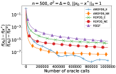
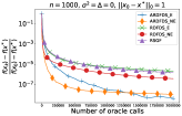
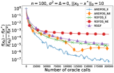
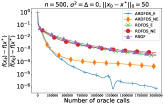
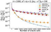
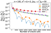
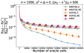
Figure 1: Numerical results for minimizing Nesterov’s function for different sparsity levels of $x_{0}-x^{*}$ and dimensions $n$ of the problem.

As the theory predicts, our methods with $p=1$ work increasingly better than our methods with $p=2$ as $n$ is growing when $\|x_{0}-x^{*}\|_{0}$ is small.

3.1.2 Experiments with different variance

In this subsection we report the numerical results with different values of $\sigma^{2}$. For each choice of the dimension $n$ we used two values of $\sigma^{2}$: $\sigma_{\text{small}}^{2}=\tfrac{\varepsilon^{\nicefrac{{3}}{{2}}}\sqrt{nL_{2}}}{\|x_{0}-x^{*}\|_{1}}$ and $\sigma_{\text{big}}^{2}=10000\sigma_{\text{small}}^{2}$ with $\varepsilon=10^{-3}$. As one can see from Table 2, when $\sigma^{2}=\sigma_{\text{small}}^{2}$ the first term under the maximum in the complexity bound is dominating (up to logarithmic factors). This implies that ARDFDS with $p=1$ is guaranteed to find an $\varepsilon$-solution even with the mini-batch size $m=1$ (up to logarithmical factors). We choose $\varepsilon=10^{-3}$, $\Delta=0$ and $x_{0}$ such that it differs from $x^{*}$ only in the first component and run the experiments for $n=100,500,1000$ and $\sigma^{2}=\sigma_{\text{small}}^{2},\sigma_{\text{big}}^{2}$, see Figures 2 and 3.

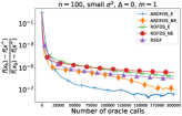
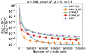
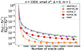
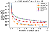
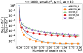
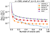
Figure 2: Numerical results for minimizing Nesterov’s function with noisy stochastic oracle having $\sigma^{2}=\sigma_{\text{small}}^{2}$ for different sizes of mini-batch $m$ and dimensions of the problem $n$.

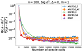
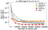
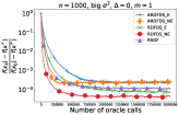
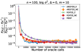
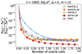
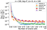
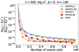
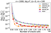
Figure 3: Numerical results for minimizing Nesterov’s function with noisy stochastic oracle having $\sigma^{2}=\sigma_{\text{big}}^{2}$ for different sizes of mini-batch $m$ and dimensions of the problem $n$.

We see in Figure 2 that for $\sigma^{2}=\sigma_{\text{small}}^{2}$ it is sufficient to use mini-batches of the size $m=1$ to reach accuracy $\varepsilon=10^{-3}$ and the overall picture is very similar to the one presented in Figure 1.

In contrast, when $\sigma^{2}=\sigma_{\text{big}}^{2}$ (Figure 3) and $m=1$ the methods fail to reach the target accuracy. In these tests accelerated methods show higher sensitivity to the noise and, as a consequence, we see that for $n=500,1000$ and $m=10$ RDFDS_NE reaches the accuracy $\varepsilon=10^{-3}$ faster than competitors justifying the following insight that we have from our theory: when the variance is large, non-accelerated methods require smaller mini-batch size $m$ and are able to find $\varepsilon$-solution faster than their accelerated counterparts.

3.1.3 Experiments with different noise level of the oracle

Here we present the numerical experiments with different values of $\Delta$. To isolate the effect of the non-stochastic noise, we set $\sigma=0$ for all tests reported in this subsection. We run the methods for problems with $n=100,500,1000$ and chose the starting point in the same way as in Subsection 3.1.2. For each choice of the dimension $n$ we used three values of $\Delta$: $\Delta_{\text{small}}=\min\left\{\tfrac{\varepsilon^{3/2}\sqrt{2}}{\sqrt{L_{2}\|x_{0}-x^{*}\|_{1}^{2}n\ln n}},\,\tfrac{2\varepsilon^{2}}{nL_{2}\|x_{0}-x^{*}\|_{1}^{2}}\right\}$, $\Delta_{\text{medium}}=10^{3}\cdot\Delta_{\text{small}}$ and $\Delta_{\text{large}}=10^{6}\cdot\Delta_{\text{small}}$ with $\varepsilon=10^{-3}$. As one can see from Table 2 when $\Delta=\Delta_{\text{small}}$ ARDFDS with $p=1$ is guaranteed to find an $\varepsilon$-solution. The results are reported in Figure 4.

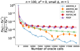
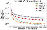
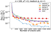
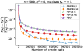
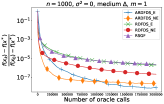
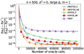
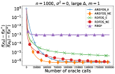
Figure 4: Numerical results for minimizing Nesterov’s function with noisy stochastic oracle having $\sigma^{2}=0$ for different $\Delta$ and dimensions of the problem $n$.

We see that for larger values of $\Delta$ accelerated methods achieve worse accuracy than for small values of $\Delta$. However, in all experiments our methods succeeded to reach $\varepsilon$-solution with $\varepsilon=10^{-3}$ meaning that the noise level $\Delta$ in practice can be much larger than it is prescribed by our theory.

3.1.4 Experiment with large dimension

In Figure 5 we report the experiment results for $n=5000$, $\sigma^{2}=\sigma_{\text{small}}^{2}=\tfrac{\varepsilon^{\nicefrac{{3}}{{2}}}\sqrt{nL_{2}}}{\|x_{0}-x^{*}\|_{1}}$,
$\Delta=\Delta_{\text{small}}=\min\left\{\tfrac{\varepsilon^{3/2}\sqrt{2}}{\sqrt{L_{2}\|x_{0}-x^{*}\|_{1}^{2}n\ln n}},\,\tfrac{2\varepsilon^{2}}{nL_{2}\|x_{0}-x^{*}\|_{1}^{2}}\right\}$, and $\varepsilon=10^{-3}$.

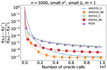
Figure 5: Numerical results for minimizing Nesterov’s function with noisy stochastic oracle having $\sigma^{2}=\sigma_{\text{small}}^{2}$ and $\Delta=\Delta_{\text{small}}$ for the dimension of the problem $n=5000$.

The obtained results are in a good agreement with our theory and experiment results for smaller dimensions.

3.2 Experiments with logistic regression

In this subsection we report the numerical results for our methods applied to the logistic regression problem:

(45) $$\min\limits_{x\in\mathbb{R}^{n}}\left\{f(x)=\frac{1}{M}\sum\limits_{i=1}^{M}f_{i}(x)\right\},\quad f_{i}(x)=\log\left(1+\exp\left(-y_{i}\cdot(Ax)_{i}\right)\right).$$

Here $f_{i}(x)$ is the loss on the $i$-th data point, $A\in\mathbb{R}^{M\times n}$ is a matrix of instances, $y\in\{-1,1\}^{M}$ is a vector of labels and $x\in\mathbb{R}^{n}$ is a vector of parameters (or weights). It can be easily shown that $f(x)$ is convex and $L_{2}$-smooth w.r.t. the Euclidean norm with $L_{2}=\nicefrac{{\sqrt{\lambda_{\max}(A^{\top}A)}}}{{4M}}$ where $\lambda_{\max}(A^{\top}A)$ denotes the maximal eigenvalue of $A^{\top}A$. Moreover, problem (45) is a special case of (1) with $\xi$ being a random variable with the uniform distribution on $\{1,\ldots,M\}$.

For our experiments we use the data from LIBSVM library [20], see also Table 6 summarizing the information about the datasets we used.

	heart	diabetes	a9a	phishing	w8a
Size $M$	$270$	$768$	$32561$	$11055$	$49749$
Dimension $n$	$13$	$8$	$123$	$68$	$300$

Table 6: Summary of used datasets.

In all test we chose $t=10^{-8}$ and the starting point $x_{0}$ such that it differs from $x^{*}$ only in the first component and $f(x_{0})-f(x^{*})\sim 10$. We use standard solvers from scipy library to obtain a very good approximation of a solution $x^{*}$ and use it to measure the quality of the approximations by other algorithms. The results for the batch (and hence deterministic) methods with $m=M$ and mini-batch stochastic methods are presented in Figures 6 and 7 respectively.

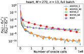
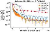
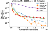
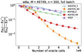
Figure 6: Numerical results for solving logistic regression problem (45) for different datasets using batch methods with $m=M$.

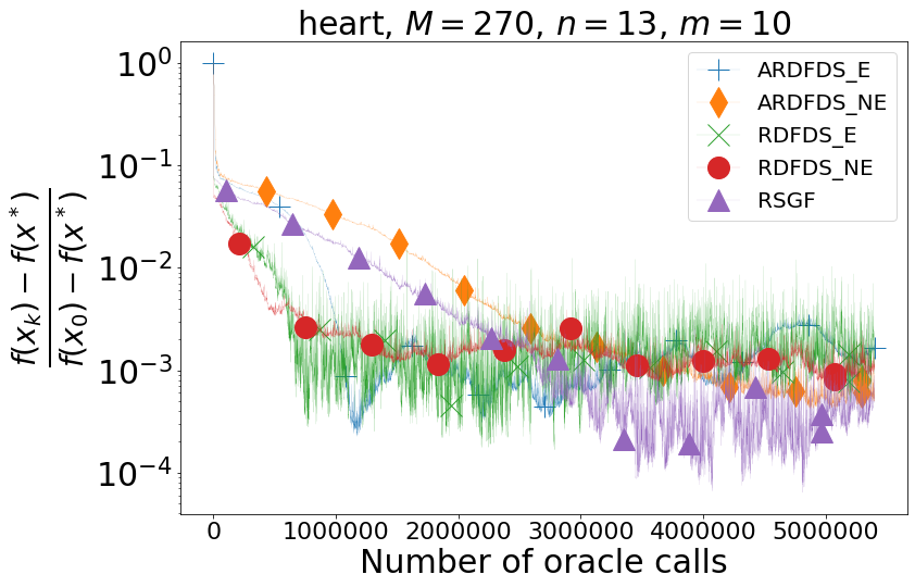
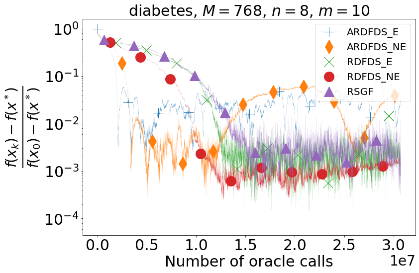
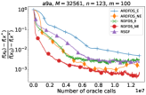
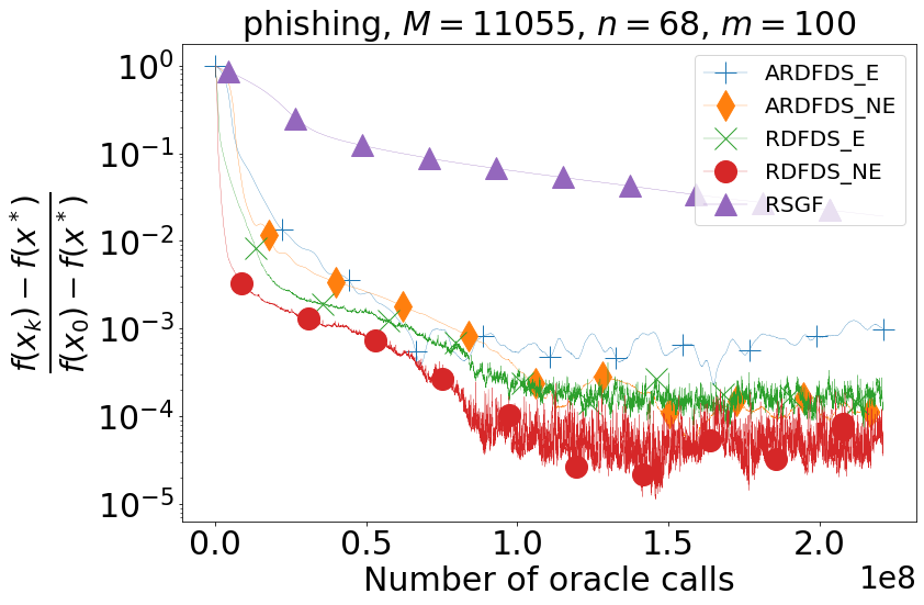
Figure 7: Numerical results for solving logistic regression problem (45) for different datasets using mini-batch stochastic methods.

In all cases methods with the $1$-norm proximal setup show the best or comparable with the best results.

4 Conclusion

In this paper, we propose two new algorithms for stochastic smooth derivative-free convex optimization with two-point feedback and inexact function values oracle. Our first algorithm is an accelerated one and the second one is a non-accelerated one. Notably, despite the traditional choice of $2$-norm proximal setup for unconstrained optimization problems, our analysis has yielded better complexity bounds for the method with $1$-norm proximal setup than the ones with $2$-norm proximal setup. This is also confirmed by numerical experiments.

Appendix A Proof of Lemma 2.1

In this appendix we prove that, for $e\in RS_{2}\left(1\right)$, $q\geqslant 2$, and $n\geqslant 8$,

(46) $$\mathbb{E}[\|e\|_{q}^{2}] \leqslant\min\{q-1,\,16\ln n-8\}n^{\tfrac{2}{q}-1},$$

(47) $$\mathbb{E}[\langle s,\,e\rangle^{2}\|e\|_{q}^{2}] \leqslant 6\|s\|_{2}^{2}\min\{q-1,16\ln n-8\}n^{\tfrac{2}{q}-2}.$$

Throughout this appendix, to simplify the notation, we denote by $\mathbb{E}$ the expectation w.r.t. random vector $e\in RS_{2}\left(1\right)$.

We start by proving the following inequality, which could be not tight for large $q$:

(48) $$\mathbb{E}[\|e\|_{q}^{2}]\leqslant(q-1)n^{\tfrac{2}{q}-1},\quad 2\leqslant q<\infty.$$

We have

(49) $$\begin{array}[]{c}\mathbb{E}[\|e\|_{q}^{2}]=\mathbb{E}\left[\left(\sum\limits_{k=1}^{n}|e_{k}|^{q}\right)^{\tfrac{2}{q}}\right]\overset{\text{\char 172}}{\leqslant}\left(\mathbb{E}\left[\sum\limits_{k=1}^{n}|e_{k}|^{q}\right]\right)^{\tfrac{2}{q}}\overset{\text{\char 173}}{=}\left(n\mathbb{E}[|e_{2}|^{q}]\right)^{\tfrac{2}{q}},\end{array}$$

where ① is due to probabilistic version of Jensen’s inequality (function $\varphi(x)=x^{\tfrac{2}{q}}$ is concave, because $q\geqslant 2$) and ② is because expectation is linear and components of the vector $e$ are identically distributed. We also denote by $e_{k}$ the $k$-th component of $e$. In particular, $e_{2}$ is the second component.

By the Poincare lemma, $e$ has the same distribution as $\tfrac{\xi}{\sqrt{\xi_{1}^{2}+\dots+\xi_{n}^{2}}}$, where $\xi$ is the standard Gaussian random vector with zero mean and identity covariance matrix. Then

$$\begin{array}[]{rl}\mathbb{E}[|e_{2}|^{q}]&=\mathbb{E}\left[\tfrac{|\xi_{2}|^{q}}{\left(\xi_{1}^{2}+\ldots+\xi_{n}^{2}\right)^{\tfrac{q}{2}}}\right]\\ &=\idotsint\limits_{\mathbb{R}^{n}}|x_{2}|^{q}\left(\sum\limits_{k=1}^{n}x_{k}^{2}\right)^{-\tfrac{q}{2}}\cdot\tfrac{1}{(2\pi)^{\tfrac{n}{2}}}\cdot\exp\left(-\tfrac{1}{2}\sum\limits_{k=1}^{n}x_{k}^{2}\right)dx_{1}\ldots dx_{n}.\end{array}$$

For the transition to the spherical coordinates

$$\begin{array}[]{rl}x_{1}&=r\cos\varphi\sin\theta_{1}\ldots\sin\theta_{n-2},\quad x_{2}=r\sin\varphi\sin\theta_{1}\ldots\sin\theta_{n-2},\\ x_{3}&=r\cos\theta_{1}\sin\theta_{2}\ldots\sin\theta_{n-2},\quad x_{4}=r\cos\theta_{2}\sin\theta_{3}\ldots\sin\theta_{n-2},\\ &\ldots\\ x_{n}&=r\cos\theta_{n-2},\quad r>0,\,\varphi\in[0,2\pi),\,\theta_{i}\in[0,\pi],\,{\color[rgb]{0,0,0}i=1,...,n-2}\end{array}$$

the Jacobian satisfies

$$\det\left(\tfrac{\partial(x_{1},\ldots,x_{n})}{\partial(r,\varphi,\theta_{1},\theta_{2},\ldots,\theta_{n-2})}\right)=r^{n-1}\sin\theta_{1}(\sin\theta_{2})^{2}\ldots(\sin\theta_{n-2})^{n-2}.$$

In the new coordinates we have

$$\begin{array}[]{rl}\mathbb{E}[|e_{2}|^{q}]&=\idotsint\limits_{\begin{subarray}{c}r>0,\,\varphi\in[0,2\pi),\\ \theta_{i}\in[0,\pi],\,i={\color[rgb]{0,0,0}1,...,n-2}\end{subarray}}r^{n-1}|\sin\varphi|^{q}|\sin\theta_{1}|^{q+1}|\sin\theta_{2}|^{q+2}\ldots|\sin\theta_{n-2}|^{q+n-2}\\ &\cdot\tfrac{{\color[rgb]{0,0,0}\exp{(-\tfrac{r^{2}}{2}})}}{(2\pi)^{\tfrac{n}{2}}}dr\ldots d\theta_{n-2}=\tfrac{1}{(2\pi)^{\tfrac{n}{2}}}I_{r}\cdot I_{\varphi}\cdot I_{\theta_{1}}\cdot I_{\theta_{2}}\cdot\ldots\cdot I_{\theta_{n-2}},\end{array}$$

where $I_{r}=\int\limits_{0}^{+\infty}r^{n-1}{\color[rgb]{0,0,0}\exp\left({-\tfrac{r^{2}}{2}}\right)}dr$,
$I_{\varphi}=\int\limits_{0}^{2\pi}|\sin\varphi|^{q}d\varphi=2\int\limits_{0}^{\pi}|\sin\varphi|^{q}d\varphi$, $I_{\theta_{i}}=\int\limits_{0}^{\pi}|\sin\theta_{i}|^{q+i}d\theta_{i}$ for ${\color[rgb]{0,0,0}i=1,...,n-2}$. Next we calculate these integrals starting with $I_{r}$:

$$\begin{array}[]{c}I_{r}=\int\limits_{0}^{+\infty}r^{n-1}{\color[rgb]{0,0,0}\exp\left({-\tfrac{r^{2}}{2}}\right)}dr\overset{{\color[rgb]{0,0,0}r=\sqrt{2t}}}{=}\int\limits_{0}^{+\infty}(2t)^{\tfrac{n}{2}-1}{\color[rgb]{0,0,0}\exp\left(-t\right)}dt=2^{\tfrac{n}{2}-1}\Gamma(\tfrac{n}{2}).\end{array}$$

To compute the other integrals, we consider the following integral for $\alpha>0$:

$$\begin{array}[]{rl}\int\limits_{0}^{\pi}|\sin\varphi|^{\alpha}d\varphi&=2\int\limits_{0}^{\tfrac{\pi}{2}}|\sin\varphi|^{\alpha}d\varphi=2\int\limits_{0}^{\tfrac{\pi}{2}}(\sin^{2}\varphi)^{\tfrac{\alpha}{2}}d\varphi\\ &\overset{{\color[rgb]{0,0,0}t=\sin^{2}\varphi}}{=}\int\limits_{0}^{1}t^{\tfrac{\alpha-1}{2}}(1-t)^{-\tfrac{1}{2}}dt=B(\tfrac{\alpha+1}{2},\,\tfrac{1}{2})=\tfrac{\Gamma(\tfrac{\alpha+1}{2})\Gamma(\tfrac{1}{2})}{\Gamma(\tfrac{\alpha+2}{2})}=\sqrt{\pi}\tfrac{\Gamma(\tfrac{\alpha+1}{2})}{\Gamma(\tfrac{\alpha+2}{2})}.\end{array}$$

This gives

(50) $$\begin{array}[]{rl}\mathbb{E}[|e_{2}|^{q}]=\tfrac{1}{(2\pi)^{\tfrac{n}{2}}}I_{r}\cdot I_{\varphi}\cdot I_{\theta_{1}}\cdot I_{\theta_{2}}\cdot\ldots\cdot I_{\theta_{n-2}}\\ =\tfrac{1}{(2\pi)^{\tfrac{n}{2}}}\cdot 2^{\tfrac{n}{2}-1}\Gamma(\tfrac{n}{2})\cdot 2\sqrt{\pi}\tfrac{\Gamma(\tfrac{q+1}{2})}{\Gamma(\tfrac{q+2}{2})}\cdot\sqrt{\pi}\tfrac{\Gamma(\tfrac{q+2}{2})}{\Gamma(\tfrac{q+3}{2})}\cdot\ldots\cdot\sqrt{\pi}\tfrac{\Gamma(\tfrac{q+n-1}{2})}{\Gamma(\tfrac{q+n}{2})}=\tfrac{1}{\sqrt{\pi}}\cdot\tfrac{\Gamma(\tfrac{n}{2})\Gamma(\tfrac{q+1}{2})}{\Gamma(\tfrac{q+n}{2})}.\end{array}$$

The next step is to show that, for all $q\geqslant 2$,

(51) $$\tfrac{1}{\sqrt{\pi}}\cdot\tfrac{\Gamma(\tfrac{n}{2})\Gamma(\tfrac{q+1}{2})}{\Gamma(\tfrac{q+n}{2})}\leqslant\left(\tfrac{q-1}{n}\right)^{\tfrac{q}{2}}.$$

First we show that (51) holds for $q=2$ and arbitrary $n$:

$$\tfrac{1}{\sqrt{\pi}}\cdot\tfrac{\Gamma(\tfrac{n}{2})\Gamma(\tfrac{2+1}{2})}{\Gamma(\tfrac{2+n}{2})}-\tfrac{1}{n}=\tfrac{1}{\sqrt{\pi}}\cdot\tfrac{\Gamma(\tfrac{n}{2})\cdot\tfrac{1}{2}\Gamma(\tfrac{1}{2})}{\tfrac{n}{2}\Gamma(\tfrac{n}{2})}-\tfrac{1}{n}=\tfrac{1}{n}-\tfrac{1}{n}=0\leqslant 0.$$

Next, we consider the function $f_{n}(q)=\tfrac{1}{\sqrt{\pi}}\cdot\tfrac{\Gamma(\tfrac{n}{2})\Gamma(\tfrac{q+1}{2})}{\Gamma(\tfrac{q+n}{2})}-\left(\tfrac{q-1}{n}\right)^{\tfrac{q}{2}}$, where $q\geqslant 2$, and digamma function $\psi(x)=\tfrac{d(\ln(\Gamma(x)))}{dx}$ with scalar argument $x>0$. For the gamma function it holds that $\Gamma(x+1)=x\Gamma(x),\,x>0.$ Taking natural logarithm in both sides and derivative w.r.t. $x$, we get $\tfrac{d(\ln(\Gamma(x+1)))}{dx}=\tfrac{d(\ln(\Gamma(x)))}{dx}+\tfrac{1}{x}$, meaning that $\psi(x+1)=\psi(x)+\tfrac{1}{x}.$ To prove that the digamma function monotonically increases for $x>0$, we show that

(52) $$\left(\Gamma^{\prime}(x)\right)^{2}<\Gamma(x)\Gamma^{\prime\prime}(x).$$

Indeed,

$$\begin{array}[]{rl}\left(\Gamma^{\prime}(x)\right)^{2}&=\left(\int\limits_{0}^{+\infty}{\color[rgb]{0,0,0}\exp(-t)}\ln t\cdot t^{x-1}dt\right)^{2}\\ &\overset{\text{\char 172}}{<}\int\limits_{0}^{+\infty}\left({\color[rgb]{0,0,0}\exp(-\tfrac{t}{2})}t^{\tfrac{x-1}{2}}\right)^{2}dt\cdot\int\limits_{0}^{+\infty}\left({\color[rgb]{0,0,0}\exp(-\tfrac{t}{2})}t^{\tfrac{x-1}{2}}\ln t\right)^{2}dt\\ &=\int\limits_{0}^{+\infty}{\color[rgb]{0,0,0}\exp(-t)}t^{x-1}dt\cdot\int\limits_{0}^{+\infty}{\color[rgb]{0,0,0}\exp(t)}t^{x-1}\ln^{2}tdt=\Gamma(x)\Gamma^{\prime\prime}(x),\end{array}$$

where ① follows from the Cauchy-Schwartz inequality and we have strict inequality since functions ${\color[rgb]{0,0,0}\exp(-\tfrac{t}{2})}t^{\tfrac{x-1}{2}}$ and ${\color[rgb]{0,0,0}\exp(-\tfrac{t}{2})}t^{\tfrac{x-1}{2}}\ln t$ are linearly independent. From (52) it follows that $\tfrac{d^{2}(\ln\Gamma(x))}{dx^{2}}=\left(\tfrac{\Gamma^{\prime}(x)}{\Gamma(x)}\right)^{\prime}=\tfrac{\Gamma^{\prime\prime}(x)}{\Gamma(x)}-\tfrac{\left(\Gamma^{\prime}(x)\right)^{2}}{\left(\Gamma(x)\right)^{2}}\overset{\eqref{lemm1:digamma_decrease}}{>}0,$ i.e. digamma function is increasing.

Now we show that $f_{n}(q)$ decreases on the interval $[2,+\infty)$. To that end, we consider $\ln(f_{{\color[rgb]{0,0,0}n}}(q))$

$$\begin{array}[]{rl}\ln(f_{n}(q))&=\ln\left(\tfrac{\Gamma(\tfrac{n}{2})}{\sqrt{\pi}}\right)+\ln\left(\Gamma\left(\tfrac{q+1}{2}\right)\right)-\ln\left(\Gamma\left(\tfrac{q+n}{2}\right)\right)-\tfrac{q}{2}\left(\ln(q-1)-\ln n\right),\\ \tfrac{d(\ln(f_{n}(q)))}{dq}&=\tfrac{1}{2}\psi\left(\tfrac{q+1}{2}\right)-\tfrac{1}{2}\psi\left(\tfrac{q+n}{2}\right)-\tfrac{1}{2}\ln(q-1)-\tfrac{q}{2(q-1)}+\tfrac{1}{2}\ln n\end{array}$$

and show that $\tfrac{d(\ln(f_{n}(q)))}{dq}<0$ for $q\geqslant 2$. Let $k=\lfloor\tfrac{n}{2}\rfloor$ (the largest integer which is no greater than $\tfrac{n}{2}$). Then $\psi\left(\tfrac{q+n}{2}\right)>\psi\left(k-1+\tfrac{q+1}{2}\right)$ and $\ln n\leqslant\ln(2k+1)$, whence,

$$\begin{array}[]{rl}\tfrac{d(\ln(f_{n}(q)))}{dq}&<\tfrac{1}{2}\left(\psi\left(\tfrac{q+1}{2}\right)-\psi\left(k-1+\tfrac{q+1}{2}\right)\right)-\tfrac{1}{2}\ln(q-1)-\tfrac{q}{2(q-1)}+\tfrac{1}{2}\ln(2k+1)\\ &=\tfrac{1}{2}\left(\psi\left(\tfrac{q+1}{2}\right)-\sum\limits_{i=1}^{k-1}\tfrac{1}{\tfrac{q+1}{2}+k-i-1}-\psi\left(\tfrac{q+1}{2}\right)\right)-\tfrac{q}{2(q-1)}+\tfrac{1}{2}\ln\left(\tfrac{2k+1}{q-1}\right)\\ &\overset{\text{\char 172}}{\leqslant}-\tfrac{1}{2}\sum\limits_{i=1}^{k-1}\tfrac{2}{q-1+2k-2i}-\tfrac{1}{q-1}+\tfrac{1}{2}\ln\left(\tfrac{2k+1}{q-1}\right)\\ &=-\tfrac{1}{2}\left(\tfrac{2}{q-1}+\tfrac{2}{q+1}+\tfrac{2}{q+3}+\ldots+\tfrac{2}{q+2k-3}\right)+\tfrac{1}{2}\ln\left(\tfrac{2k+1}{q-1}\right)\\ &\overset{\text{\char 173}}{<}-\tfrac{1}{2}\ln\left(\tfrac{q+2k-1}{q-1}\right)+\tfrac{1}{2}\ln\left(\tfrac{2k+1}{q-1}\right)\overset{\text{\char 174}}{\leqslant}-\tfrac{1}{2}\ln\left(\tfrac{2k+1}{q-1}\right)+\tfrac{1}{2}\ln\left(\tfrac{2k+1}{q-1}\right)=0,\end{array}$$

where ① and ③ are since $q\geqslant 2$, ② follows from an estimate of the integral of $\tfrac{1}{x}$ by the integral of the constant functions $g_{i}(x)=\tfrac{1}{q-1+2i},\,x\in[q-1+2i,q-1+2i+2],\,i={\color[rgb]{0,0,0}0,...,2k-1}$: $\tfrac{2}{q-1}+\tfrac{2}{q+1}+\tfrac{2}{q+3}+\ldots+\tfrac{2}{q+2k-3}>\int\limits_{q-1}^{q+2k-1}\tfrac{1}{x}dx=\ln\left(\tfrac{q+2k-1}{q-1}\right).$

Thus, we have shown that $\tfrac{d(\ln(f_{n}(q)))}{dq}<0$ for $q\geqslant 2$ and an arbitrary natural number $n$. Therefore, for any fixed number $n$, the function $f_{n}(q)$ decreases as $q$ increases, which means that $f_{n}(q)\leqslant f_{n}(2)=0$, i.e., (51) holds. From this, (49), and (50) we obtain (48), i.e. that, for all $2\leqslant q<\infty$,

(53) $$\mathbb{E}[||e||_{q}^{2}]\overset{\eqref{lemm1:jensen}}{\leqslant}\left(n\mathbb{E}[|e_{2}|^{q}]\right)^{\tfrac{2}{q}}\overset{\eqref{lemm1:expectation_component},\eqref{lemm1:key_estimation}}{\leqslant}(q-1)n^{\tfrac{2}{q}-1}.$$

Next, we analyze separately the case of large $q$, in particular, $q=\infty$. We consider the r.h.s. of (53) as a function of $q$ and find its minimum for $q\geqslant 2$. Denote $h_{n}(q)=\ln(q-1)+\left(\tfrac{2}{q}-1\right)\ln n$, which is the logarithm of the r.h.s. of (53). The derivative of $h_{n}(q)$ is $\tfrac{dh_{n}(q)}{dq}=\tfrac{1}{q-1}-\tfrac{2\ln n}{q^{2}}$, which implies that the first-order optimality condition is $\tfrac{1}{q-1}-\tfrac{2\ln n}{q^{2}}=0,$ or equivalently $q^{2}-2q\ln n+2\ln n=0$. If $n\geqslant 8$, then the function $h_{n}(q)$ attains its minimum on the set $[2,+\infty)$ at $q_{0}=\ln n\left(1+\sqrt{1-\tfrac{2}{\ln n}}\right)$ (for the case $n\leqslant 7$ the optimal point is $q_{0}=2$ and without loss of generality, we assume $n\geqslant 8$). Therefore, for all $q>q_{0}$, including $q=\infty$, we have

(54) $$\begin{array}[]{rl}\mathbb{E}[||e||_{q}^{2}]&\overset{\text{\char 172}}{<}\mathbb{E}[||e||_{q_{0}}^{2}]\overset{\eqref{lemm1:pre-final}}{\leqslant}(q_{0}-1)n^{\tfrac{2}{q_{0}}-1}\overset{\text{\char 173}}{\leqslant}(2\ln n-1)n^{\tfrac{2}{\ln n}-1}\\ &=(2\ln n-1)\tfrac{{\color[rgb]{0,0,0}\exp(2)}}{n}\leqslant(16\ln n-8)\tfrac{1}{n}\leqslant(16\ln n-8)n^{\tfrac{2}{q}-1},\end{array}$$

where ① is since $\|e\|_{q}<\|e\|_{q_{0}}$ for $q>q_{0}$, ② follows from $q_{0}\leqslant 2\ln n,\,q_{0}\geqslant\ln n$. Combining estimates (53) and (54), we obtain (46).

It remains to prove (47). First, we estimate $\sqrt{\mathbb{E}[\|e\|_{q}^{4}]}$. By the probabilistic Jensen’s inequality, for $q\geqslant 2$,

$$\begin{array}[]{rl}\mathbb{E}[||e||_{q}^{4}]&=\mathbb{E}\left[\left(\left(\sum\limits_{k=1}^{n}|e_{k}|^{q}\right)^{2}\right)^{\tfrac{2}{q}}\right]\leqslant\left(\mathbb{E}\left[\left(\sum\limits_{k=1}^{n}|e_{k}|^{q}\right)^{2}\right]\right)^{\tfrac{2}{q}}\\ &\overset{\text{\char 172}}{\leqslant}\left(\mathbb{E}\left[\left(n\sum\limits_{k=1}^{n}|e_{k}|^{2q}\right)\right]\right)^{\tfrac{2}{q}}\overset{\text{\char 173}}{=}\left(n^{2}\mathbb{E}[|e_{2}|^{2q}]\right)^{\tfrac{2}{q}}\\ &\overset{\eqref{lemm1:expectation_component},\eqref{lemm1:key_estimation}}{\leqslant}n^{\tfrac{4}{q}}\left(\left(\tfrac{2q-1}{n}\right)^{\tfrac{2q}{2}}\right)^{\tfrac{2}{q}}=(2q-1)^{2}n^{\tfrac{4}{q}-2},\end{array}$$

where ① is since $\left(\sum\limits_{k=1}^{n}x_{k}\right)^{2}\leqslant n\sum\limits_{k=1}^{n}x_{k}^{2}$ for $x_{1},x_{2},\ldots,x_{n}\in\mathbb{R}$ and ② follows from the linearity of expectation and the components of the random vector $e$ being identically distributed. From this we obtain

(55) $$\sqrt{\mathbb{E}[||e||_{q}^{4}]}\leqslant(2q-1)n^{\tfrac{2}{q}-1}.$$

Next, we consider the r.h.s. of (55) as a function of $q$ and find its minimum for $q\geqslant 2$. The logarithm of the r.h.s. of (55) is $h_{n}(q)=\ln(2q-1)+\left(\tfrac{2}{q}-1\right)\ln n$ with the derivative $\tfrac{dh_{n}(q)}{dq}=\tfrac{2}{2q-1}-\tfrac{2\ln n}{q^{2}}$, which implies the first-order optimality condition $\tfrac{2}{2q-1}-\tfrac{2\ln n}{q^{2}}=0$, or equivalently $q^{2}-2q\ln n+\ln n=0$. If $n\geqslant 3$, the point where the function $h_{n}(q)$ attains its minimum on the set $[2,+\infty)$ is $q_{0}=\ln n\left(1+\sqrt{1-\tfrac{1}{\ln n}}\right)$ (for the case $n\leqslant 2$ the optimal point is $q_{0}=2$ and without loss of generality we assume that $n\geqslant 3$). Therefore for all $q>q_{0}$, including $q=\infty$,

(56) $$\begin{array}[]{rl}\sqrt{\mathbb{E}[\|e\|_{q}^{4}]}&\overset{\text{\char 172}}{<}\sqrt{\mathbb{E}[\|e\|_{q_{0}}^{4}]}\overset{\eqref{lemm1:pre_final_q_norm_power4}}{\leqslant}(2q_{0}-1)n^{\tfrac{2}{q_{0}}-1}\overset{\text{\char 173}}{\leqslant}(4\ln n-1)n^{\tfrac{2}{\ln n}-1}\\ &=(4\ln n-1)\tfrac{{\color[rgb]{0,0,0}\exp(2)}}{n}\leqslant(32\ln n-8)\tfrac{1}{n}\leqslant(32\ln n-8)n^{\tfrac{2}{q}-1},\end{array}$$

where ① is since $\|e\|_{q}<\|e\|_{q_{0}}$ for $q>q_{0}$, ② follows from $q_{0}\leqslant 2\ln n,\,q_{0}\geqslant\ln n$. Combining the estimates (55) and (56), we get the inequality

(57) $$\sqrt{\mathbb{E}[\|e\|_{q}^{4}]}\leqslant\min\{2q-1,32\ln n-8\}n^{\tfrac{2}{q}-1}.$$

The next step is to estimate $\mathbb{E}[\langle s,\,e\rangle^{4}]$, where $s\in\mathbb{R}^{n}$ is some fixed vector. Let $S_{n}(r)$ be the surface area of $n$-dimensional Euclidean sphere with radius $r$ and $d\sigma(e)$ be unnormalized uniform measure on $n$-dimensional Euclidean sphere. Then $S_{n}(r)=S_{n}(1)r^{n-1},\,\tfrac{S_{n-1}(1)}{S_{n}(1)}=\tfrac{n-1}{n\sqrt{\pi}}\tfrac{\Gamma(\tfrac{n+2}{2})}{\Gamma(\tfrac{n+1}{2})}$. Let $\varphi$ be the angle between $s$ and $e$. Then

(58) $$\begin{array}[]{rl}&\mathbb{E}[\langle s,\,e\rangle^{4}]=\tfrac{1}{S_{n}(1)}\int\limits_{S}\langle s,\,e\rangle^{4}d\sigma(\varphi)=\tfrac{1}{S_{n}(1)}\int\limits_{0}^{\pi}\|s\|_{2}^{4}\cos^{3}\varphi S_{n-1}(\sin\varphi)d\varphi\\ &=\|s\|_{2}^{4}\tfrac{S_{n-1}(1)}{S_{n}(1)}\int\limits_{0}^{\pi}\cos^{4}\varphi\sin^{n-2}\varphi d\varphi=\|s\|_{2}^{4}\cdot\tfrac{n-1}{n\sqrt{\pi}}\tfrac{\Gamma(\tfrac{n+2}{2})}{\Gamma(\tfrac{n+1}{2})}\int\limits_{0}^{\pi}\cos^{4}\varphi\sin^{n-2}\varphi d\varphi.\end{array}$$

Further, denoting the Beta function by $B(\cdot,\cdot)$,

$$\begin{array}[]{rl}&\int\limits_{0}^{\pi}\cos^{4}\varphi\sin^{n-2}\varphi d\varphi=2\int\limits_{0}^{\tfrac{\pi}{2}}\cos^{4}\varphi\sin^{n-2}\varphi d\varphi\overset{{\color[rgb]{0,0,0}t=\sin^{2}\varphi}}{=}\int\limits_{0}^{\tfrac{\pi}{2}}t^{\tfrac{n-3}{2}}(1-t)^{\tfrac{3}{2}}dt\\ &=B(\tfrac{n-1}{2},\tfrac{5}{2})=\tfrac{\Gamma(\tfrac{5}{2})\Gamma(\tfrac{n-1}{2})}{\Gamma(\tfrac{n+4}{2})}=\tfrac{\tfrac{3}{2}\cdot\tfrac{1}{2}\Gamma(\tfrac{1}{2})\Gamma(\tfrac{n-1}{2})}{\tfrac{n+2}{2}\cdot\Gamma(\tfrac{n+2}{2})}=\tfrac{3}{n+2}\cdot\tfrac{\sqrt{\pi}\Gamma(\tfrac{n-1}{2})}{2\Gamma(\tfrac{n+2}{2})}.\end{array}$$

From this and (58), we obtain

(59) $$\begin{array}[]{rl}\mathbb{E}[\langle s,\,e\rangle^{4}]&=\|s\|_{2}^{4}\cdot\tfrac{n-1}{n\sqrt{\pi}}\tfrac{\Gamma(\tfrac{n+2}{2})}{\Gamma(\tfrac{n+1}{2})}\cdot\tfrac{3}{n+2}\cdot\tfrac{\sqrt{\pi}\Gamma(\tfrac{n-1}{2})}{2\Gamma(\tfrac{n+2}{2})}\\ &=\|s\|_{2}^{4}\cdot\tfrac{3(n-1)}{2n(n+2)}\cdot\tfrac{\Gamma(\tfrac{n-1}{2})}{\tfrac{n-1}{2}\Gamma(\tfrac{n-1}{2})}=\tfrac{3\|s\|_{2}^{4}}{n(n+2)}\overset{\text{\char 172}}{\leqslant}\tfrac{3\|s\|_{2}^{4}}{n^{2}}.\end{array}$$

To prove (47), it remains to use (57), (59) and the Cauchy-Schwartz inequality $(\mathbb{E}[XY])^{2}\leqslant\mathbb{E}[X^{2}]\cdot\mathbb{E}[Y^{2}]$:

$$\begin{array}[]{c}\mathbb{E}[\langle s,\,e\rangle^{2}||e||_{q}^{2}]\leqslant\sqrt{\mathbb{E}[\langle s,\,e\rangle^{4}]\cdot\mathbb{E}[\|e\|_{q}^{4}]}\leqslant\sqrt{3}\|s\|_{2}^{2}\min\{2q-1,32\ln n-8\}n^{\tfrac{2}{q}-2}.\end{array}$$

Appendix B Technical Results on Recurrent Sequences

Lemma B.1.

Let $a_{0},\ldots,a_{N-1},b,R_{1},\ldots,R_{N-1}$ be non-negative numbers and

(60) $$R_{l}\leqslant\sqrt{2}\cdot\sqrt{\left(\sum\limits_{k=0}^{l-1}a_{k}+b\sum\limits_{k=1}^{l-1}\alpha_{k+1}R_{k}\right)}\quad l=1,\ldots,N,$$

where $\alpha_{k+1}=\tfrac{k+2}{96n^{2}\rho_{n}L_{2}}$ for all $k\in\mathbb{N}$. Then, for $l=1,\ldots,N$,

(61) $$\sum\limits_{k=0}^{l-1}a_{k}+b\sum\limits_{k=1}^{l-1}\alpha_{k+1}R_{k}\leqslant\left(\sqrt{\sum\limits_{k=0}^{l-1}a_{k}}+\sqrt{2}b\cdot\tfrac{l^{2}}{96n^{2}\rho_{n}L_{2}}\right)^{2}.$$

Proof B.2.

For $l=1$ the inequality is trivial. Next we assume that (61) holds for some $l<N$ and prove this inequality for $l+1$. From the induction assumption and (60) we obtain

(62) $$\begin{array}[]{c}R_{l}\leqslant\sqrt{2}\left(\sqrt{\sum\limits_{k=0}^{l-1}a_{k}}+\sqrt{2}b\cdot\tfrac{l^{2}}{96n^{2}\rho_{n}L_{2}}\right),\end{array}$$

whence

$$\begin{array}[]{rl}&\sum\limits_{k=0}^{l}a_{k}+b\sum\limits_{k=1}^{l}\alpha_{k+1}R_{k}=\sum\limits_{k=0}^{l-1}a_{k}+b\sum\limits_{k=1}^{l-1}\alpha_{k+1}R_{k}+a_{l}+b\alpha_{l+1}R_{l}\\ &\overset{\text{\char 172}}{\leqslant}\left(\sqrt{\sum\limits_{k=0}^{l-1}a_{k}}+\sqrt{2}b\cdot\tfrac{l^{2}}{96n^{2}\rho_{n}L_{2}}\right)^{2}+a_{l}+\sqrt{2}b\alpha_{l+1}\left(\sqrt{\sum\limits_{k=0}^{l-1}a_{k}}+\sqrt{2}b\cdot\tfrac{l^{2}}{96n^{2}\rho_{n}L_{2}}\right)\\ &=\sum\limits_{k=0}^{l}a_{k}+2\sqrt{\sum\limits_{k=0}^{l-1}a_{k}}\cdot\tfrac{l^{2}\cdot\sqrt{2}b}{96n^{2}\rho_{n}L_{2}}+\tfrac{l^{4}\cdot 2b^{2}}{(96n^{2}\rho_{n}L_{2})^{2}}+\sqrt{2}b\alpha_{l+1}\left(\sqrt{\sum\limits_{k=0}^{l-1}a_{k}}+\tfrac{l^{2}\cdot\sqrt{2}b}{96n^{2}\rho_{n}L_{2}}\right)\\ &=\sum\limits_{k=0}^{l}a_{k}+2\sqrt{\sum\limits_{k=0}^{l-1}a_{k}}\cdot\sqrt{2}b\left(\tfrac{l^{2}}{96n^{2}\rho_{n}L_{2}}+\tfrac{\alpha_{l+1}}{2}\right)+2b^{2}\left(\tfrac{l^{4}}{(96n^{2}\rho_{n}L_{2})^{2}}+\cdot\tfrac{\alpha_{l+1}l^{2}}{96n^{2}\rho_{n}L_{2}}\right)\\ &\overset{\text{\char 173}}{\leqslant}\sum\limits_{k=0}^{l}a_{k}+2\sqrt{\sum\limits_{k=0}^{l}a_{k}}\tfrac{(l+1)^{2}\cdot\sqrt{2}b}{96n^{2}\rho_{n}L_{2}}+\tfrac{(l+1)^{4}\cdot 2b^{2}}{(96n^{2}\rho_{n}L_{2})^{2}}=\left(\sqrt{\sum\limits_{k=0}^{l}a_{k}}+\sqrt{2}b\cdot\tfrac{(l+1)^{2}}{96n^{2}\rho_{n}L_{2}}\right)^{2},\end{array}$$

where ① holds by the induction assumption and (62), ② is since $\sum\limits_{k=0}^{l-1}a_{k}\leqslant\sum\limits_{k=0}^{l}a_{k}$ and

$$\begin{array}[]{rl}\tfrac{l^{2}}{96n^{2}\rho_{n}L_{2}}+\tfrac{\alpha_{l+1}}{2}=\tfrac{2l^{2}+l+2}{192n^{2}\rho_{n}L_{2}}&\leqslant\tfrac{(l+1)^{2}}{96n^{2}\rho_{n}L_{2}},\\ \tfrac{l^{4}}{(96n^{2}\rho_{n}L_{2})^{2}}+\alpha_{l+1}\cdot\tfrac{l^{2}}{96n^{2}\rho_{n}L_{2}}&\leqslant\tfrac{l^{4}+(l+2)l^{2}}{(96n^{2}\rho_{n}L_{2})^{2}}\leqslant\tfrac{(l+1)^{4}}{(96n^{2}\rho_{n}L_{2})^{2}}.\end{array}$$

Lemma B.3.

Let ${\color[rgb]{0,0,0}\alpha},a_{0},\ldots,a_{N-1},b,R_{1},\ldots,R_{N-1}$ be non-negative numbers and

(63) $$R_{l}\leqslant\sqrt{2}\cdot\sqrt{\left(\sum\limits_{k=0}^{l-1}a_{k}+b\alpha\sum\limits_{k=1}^{l-1}R_{k}\right)}\quad l=1,\ldots,N.$$

Then, for $l=1,\ldots,N$,

(64) $$\sum\limits_{k=0}^{l-1}a_{k}+b\alpha\sum\limits_{k=1}^{l-1}R_{k}\leqslant\left(\sqrt{\sum\limits_{k=0}^{l-1}a_{k}}+\sqrt{2}b\alpha l\right)^{2}.$$

Proof B.4.

For $l=1$ the inequality is trivial. Next we assume that (64) holds for some $l<N$ and prove it for $l+1$. By the induction assumption and (63) we obtain

(65) $$\begin{array}[]{c}R_{l}\leqslant\sqrt{2}\left(\sqrt{\sum\limits_{k=0}^{l-1}a_{k}}+\sqrt{2}b\alpha l\right),\end{array}$$

whence

$$\begin{array}[]{rl}&\sum\limits_{k=0}^{l}a_{k}+b\alpha\sum\limits_{k=1}^{l}R_{k}=\sum\limits_{k=0}^{l-1}a_{k}+b\alpha\sum\limits_{k=1}^{l-1}R_{k}+a_{l}+b\alpha R_{l}\\ &\overset{\text{\char 172}}{\leqslant}\left(\sqrt{\sum\limits_{k=0}^{l-1}a_{k}}+\sqrt{2}b\alpha l\right)^{2}+a_{l}+\sqrt{2}b\alpha\left(\sqrt{\sum\limits_{k=0}^{l-1}a_{k}}+\sqrt{2}b\alpha l\right)\\ &=\sum\limits_{k=0}^{l}a_{k}+2\sqrt{\sum\limits_{k=0}^{l-1}a_{k}}\cdot\sqrt{2}b\alpha l+2b^{2}\alpha^{2}l^{2}+\sqrt{2}b\alpha\left(\sqrt{\sum\limits_{k=0}^{l-1}a_{k}}+\sqrt{2}b\alpha l\right)\\ &=\sum\limits_{k=0}^{l}a_{k}+2\sqrt{\sum\limits_{k=0}^{l-1}a_{k}}\cdot\sqrt{2}b\alpha\left(l+\tfrac{1}{2}\right)+2b^{2}\alpha^{2}\left(l^{2}+l\right)\\ &\overset{\text{\char 173}}{\leqslant}\sum\limits_{k=0}^{l}a_{k}+2\sqrt{\sum\limits_{k=0}^{l}a_{k}}\cdot\sqrt{2}b\alpha(l+1)+2(b\alpha(l+1))^{2}=\left(\sqrt{\sum\limits_{k=0}^{l}a_{k}}+\sqrt{2}b\alpha(l+1)\right)^{2},\end{array}$$

where ① is by the induction assumption and (65), ② is since $\sum\limits_{k=0}^{l-1}a_{k}\leqslant\sum\limits_{k=0}^{l}a_{k}$.

References

- [1] A. Agarwal, O. Dekel, and L. Xiao, Optimal algorithms for online convex optimization with multi-point bandit feedback, in COLT 2010 - The 23rd Conference on Learning Theory, 2010.
- [2] A. Agarwal, D. P. Foster, D. J. Hsu, S. M. Kakade, and A. Rakhlin, Stochastic convex optimization with bandit feedback, in Advances in Neural Information Processing Systems 24, J. Shawe-Taylor, R. S. Zemel, P. L. Bartlett, F. Pereira, and K. Q. Weinberger, eds., Curran Associates, Inc., 2011, pp. 1035–1043.
- [3] A. Akhavan, M. Pontil, and A. B. Tsybakov, Exploiting higher order smoothness in derivative-free optimization and continuous bandits, arXiv:2006.07862, (2020).
- [4] Z. Allen-Zhu and L. Orecchia, Linear coupling: An ultimate unification of gradient and mirror descent, arXiv:1407.1537, (2014).
- [5] F. Bach and V. Perchet, Highly-smooth zero-th order online optimization, in 29th Annual Conference on Learning Theory, V. Feldman, A. Rakhlin, and O. Shamir, eds., vol. 49 of Proceedings of Machine Learning Research, Columbia University, New York, New York, USA, 23–26 Jun 2016, PMLR, pp. 257–283.
- [6] P. L. Bartlett, V. Gabillon, and M. Valko, A simple parameter-free and adaptive approach to optimization under a minimal local smoothness assumption, in Proceedings of the 30th International Conference on Algorithmic Learning Theory, A. Garivier and S. Kale, eds., vol. 98 of Proceedings of Machine Learning Research, Chicago, Illinois, 22–24 Mar 2019, PMLR, pp. 184–206.
- [7] A. Bayandina, A. Gasnikov, and A. Lagunovskaya, Gradient-free two-points optimal method for non smooth stochastic convex optimization problem with additional small noise, Automation and remote control, 79 (2018). arXiv:1701.03821.
- [8] A. Belloni, T. Liang, H. Narayanan, and A. Rakhlin, Escaping the local minima via simulated annealing: Optimization of approximately convex functions, in Proceedings of The 28th Conference on Learning Theory, P. Grünwald, E. Hazan, and S. Kale, eds., vol. 40 of Proceedings of Machine Learning Research, Paris, France, 03–06 Jul 2015, PMLR, pp. 240–265.
- [9] A. Ben-Tal and A. Nemirovski, Lectures on Modern Convex Optimization (Lecture Notes), Personal web-page of A. Nemirovski, 2020, https://www2.isye.gatech.edu/~nemirovs/LMCOLN2020WithSol.pdf.
- [10] A. S. Berahas, R. H. Byrd, and J. Nocedal, Derivative-free optimization of noisy functions via quasi-Newton methods, SIAM Journal on Optimization, 29 (2019), pp. 965–993, https://doi.org/10.1137/18M1177718.
- [11] A. S. Berahas, L. Cao, K. Choromanski, and K. Scheinberg, A theoretical and empirical comparison of gradient approximations in derivative-free optimization, arXiv:1905.01332, (2019).
- [12] A. Beznosikov, E. Gorbunov, and A. Gasnikov, Derivative-free method for composite optimization with applications to decentralized distributed optimization, IFAC-PapersOnLine, (2020). Accepted, arXiv:1911.10645.
- [13] A. Beznosikov, A. Sadiev, and A. Gasnikov, Gradient-free methods for saddle-point problem, in Mathematical Optimization Theory and Operations Research 2020, A. Kononov and et al., eds., Cham, 2020, Springer International Publishing. accepted, arXiv:2005.05913.
- [14] L. Bogolubsky, P. Dvurechensky, A. Gasnikov, G. Gusev, Y. Nesterov, A. M. Raigorodskii, A. Tikhonov, and M. Zhukovskii, Learning supervised pagerank with gradient-based and gradient-free optimization methods, in Advances in Neural Information Processing Systems 29, D. D. Lee, M. Sugiyama, U. V. Luxburg, I. Guyon, and R. Garnett, eds., Curran Associates, Inc., 2016, pp. 4914–4922. arXiv:1603.00717.
- [15] R. Bollapragada and S. M. Wild, Adaptive sampling quasi-Newton methods for derivative-free stochastic optimization, arXiv:1910.13516, (2019).
- [16] R. Brent, Algorithms for Minimization Without Derivatives, Dover Books on Mathematics, Dover Publications, 1973.
- [17] S. Bubeck and N. Cesa-Bianchi, Regret analysis of stochastic and nonstochastic multi-armed bandit problems, Foundations and Trends® in Machine Learning, 5 (2012), pp. 1–122, https://doi.org/10.1561/2200000024.
- [18] S. Bubeck, Y. T. Lee, and R. Eldan, Kernel-based methods for bandit convex optimization, in Proceedings of the 49th Annual ACM SIGACT Symposium on Theory of Computing, STOC 2017, New York, NY, USA, 2017, ACM, pp. 72–85. arXiv:1607.03084.
- [19] E. J. Candes, J. K. Romberg, and T. Tao, Stable signal recovery from incomplete and inaccurate measurements, Communications on Pure and Applied Mathematics, 59 (2006), pp. 1207–1223, https://doi.org/10.1002/cpa.20124.
- [20] C.-C. Chang and C.-J. Lin, Libsvm: A library for support vector machines, ACM transactions on intelligent systems and technology (TIST), 2 (2011), pp. 1–27.
- [21] Y. Chen, A. Orvieto, and A. Lucchi, An accelerated DFO algorithm for finite-sum convex functions, in Proceedings of the 37th International Conference on Machine Learning, Proceedings of Machine Learning Research, PMLR, 2020. (accepted), arXiv:2007.03311.
- [22] K. Choromanski, A. Iscen, V. Sindhwani, J. Tan, and E. Coumans, Optimizing simulations with noise-tolerant structured exploration, in 2018 IEEE International Conference on Robotics and Automation (ICRA), 2018, pp. 2970–2977.
- [23] K. Choromanski, M. Rowland, V. Sindhwani, R. Turner, and A. Weller, Structured evolution with compact architectures for scalable policy optimization, in Proceedings of the 35th International Conference on Machine Learning, J. Dy and A. Krause, eds., vol. 80 of Proceedings of Machine Learning Research, Stockholmsmässan, Stockholm Sweden, 10–15 Jul 2018, PMLR, pp. 970–978.
- [24] A. R. Conn, K. Scheinberg, and L. N. Vicente, Introduction to Derivative-Free Optimization, Society for Industrial and Applied Mathematics, 2009, https://doi.org/10.1137/1.9780898718768.
- [25] O. Dekel, R. Eldan, and T. Koren, Bandit smooth convex optimization: Improving the bias-variance tradeoff, in Advances in Neural Information Processing Systems 28, C. Cortes, N. D. Lawrence, D. D. Lee, M. Sugiyama, and R. Garnett, eds., Curran Associates, Inc., 2015, pp. 2926–2934.
- [26] O. Devolder, Stochastic first order methods in smooth convex optimization, CORE Discussion Paper 2011/70, (2011).
- [27] O. Devolder, F. Glineur, and Y. Nesterov, First-order methods of smooth convex optimization with inexact oracle, Mathematical Programming, 146 (2014), pp. 37–75.
- [28] J. Dippon, Accelerated randomized stochastic optimization, Ann. Statist., 31 (2003), pp. 1260–1281, https://doi.org/10.1214/aos/1059655913.
- [29] D. L. Donoho, Compressed sensing, IEEE Transactions on Information Theory, 52 (2006), pp. 1289–1306.
- [30] J. C. Duchi, M. I. Jordan, M. J. Wainwright, and A. Wibisono, Optimal rates for zero-order convex optimization: The power of two function evaluations, IEEE Trans. Information Theory, 61 (2015), pp. 2788–2806. arXiv:1312.2139.
- [31] P. Dvurechensky and A. Gasnikov, Stochastic intermediate gradient method for convex problems with stochastic inexact oracle, Journal of Optimization Theory and Applications, 171 (2016), pp. 121–145, https://doi.org/10.1007/s10957-016-0999-6.
- [32] P. Dvurechensky, A. Gasnikov, and E. Gorbunov, An accelerated directional derivative method for smooth stochastic convex optimization, arXiv:1804.02394, (2018).
- [33] P. Dvurechensky, A. Gasnikov, and A. Tiurin, Randomized similar triangles method: A unifying framework for accelerated randomized optimization methods (coordinate descent, directional search, derivative-free method), arXiv:1707.08486, (2017).
- [34] V. Fabian, Stochastic approximation of minima with improved asymptotic speed, Ann. Math. Statist., 38 (1967), pp. 191–200, https://doi.org/10.1214/aoms/1177699070.
- [35] M. Fazel, R. Ge, S. Kakade, and M. Mesbahi, Global convergence of policy gradient methods for the linear quadratic regulator, in Proceedings of the 35th International Conference on Machine Learning, J. Dy and A. Krause, eds., vol. 80 of Proceedings of Machine Learning Research, Stockholmsmässan, Stockholm Sweden, 10–15 Jul 2018, PMLR, pp. 1467–1476.
- [36] A. D. Flaxman, A. T. Kalai, and H. B. McMahan, Online convex optimization in the bandit setting: Gradient descent without a gradient, in Proceedings of the Sixteenth Annual ACM-SIAM Symposium on Discrete Algorithms, SODA ’05, Philadelphia, PA, USA, 2005, Society for Industrial and Applied Mathematics, pp. 385–394.
- [37] A. Gasnikov, P. Dvurechensky, and Y. Nesterov, Stochastic gradient methods with inexact oracle, Proceedings of Moscow Institute of Physics and Technology, 8 (2016), pp. 41–91. In Russian, first appeared in arXiv:1411.4218.
- [38] A. V. Gasnikov and P. E. Dvurechensky, Stochastic intermediate gradient method for convex optimization problems, Doklady Mathematics, 93 (2016), pp. 148–151.
- [39] A. V. Gasnikov, E. A. Krymova, A. A. Lagunovskaya, I. N. Usmanova, and F. A. Fedorenko, Stochastic online optimization. single-point and multi-point non-linear multi-armed bandits. convex and strongly-convex case, Automation and Remote Control, 78 (2017), pp. 224–234, https://doi.org/10.1134/S0005117917020035. arXiv:1509.01679.
- [40] A. V. Gasnikov, A. A. Lagunovskaya, I. N. Usmanova, and F. A. Fedorenko, Gradient-free proximal methods with inexact oracle for convex stochastic nonsmooth optimization problems on the simplex, Automation and Remote Control, 77 (2016), pp. 2018–2034, https://doi.org/10.1134/S0005117916110114. arXiv:1412.3890.
- [41] S. Ghadimi and G. Lan, Stochastic first- and zeroth-order methods for nonconvex stochastic programming, SIAM Journal on Optimization, 23 (2013), pp. 2341–2368. arXiv:1309.5549.
- [42] S. Ghadimi, G. Lan, and H. Zhang, Mini-batch stochastic approximation methods for nonconvex stochastic composite optimization, Mathematical Programming, 155 (2016), pp. 267–305, https://doi.org/10.1007/s10107-014-0846-1. arXiv:1308.6594.
- [43] E. Gorbunov, D. Dvinskikh, and A. Gasnikov, Optimal decentralized distributed algorithms for stochastic convex optimization, arXiv preprint arXiv:1911.07363, (2019).
- [44] E. Hazan and K. Levy, Bandit convex optimization: Towards tight bounds, in Advances in Neural Information Processing Systems 27, Z. Ghahramani, M. Welling, C. Cortes, N. D. Lawrence, and K. Q. Weinberger, eds., Curran Associates, Inc., 2014, pp. 784–792.
- [45] K. G. Jamieson, R. Nowak, and B. Recht, Query complexity of derivative-free optimization, in Advances in Neural Information Processing Systems 25, F. Pereira, C. J. C. Burges, L. Bottou, and K. Q. Weinberger, eds., Curran Associates, Inc., 2012, pp. 2672–2680.
- [46] D. Kamzolov, P. Dvurechensky, and A. V. Gasnikov, Universal intermediate gradient method for convex problems with inexact oracle, Optimization Methods and Software, 0 (2020), pp. 1–28, https://doi.org/10.1080/10556788.2019.1711079. arXiv:1712.06036.
- [47] G. Lan, An optimal method for stochastic composite optimization, Mathematical Programming, 133 (2012), pp. 365–397. Firs appeared in June 2008.
- [48] J. Larson, M. Menickelly, and S. M. Wild, Derivative-free optimization methods, Acta Numerica, 28 (2019), p. 287–404, https://doi.org/10.1017/S0962492919000060.
- [49] T. Liang, H. Narayanan, and A. Rakhlin, On zeroth-order stochastic convex optimization via random walks, arXiv:1402.2667, (2014).
- [50] A. Locatelli and A. Carpentier, Adaptivity to smoothness in X-armed bandits, in Proceedings of the 31st Conference On Learning Theory, S. Bubeck, V. Perchet, and P. Rigollet, eds., vol. 75 of Proceedings of Machine Learning Research, PMLR, 06–09 Jul 2018, pp. 1463–1492.
- [51] A. Nemirovski, A. Juditsky, G. Lan, and A. Shapiro, Robust stochastic approximation approach to stochastic programming, SIAM Journal on Optimization, 19 (2009), pp. 1574–1609, https://doi.org/10.1137/070704277.
- [52] A. Nemirovsky and D. Yudin, Problem Complexity and Method Efficiency in Optimization, J. Wiley & Sons, New York, 1983.
- [53] Y. Nesterov, Introductory Lectures on Convex Optimization: a basic course, Kluwer Academic Publishers, Massachusetts, 2004.
- [54] Y. Nesterov, Smooth minimization of non-smooth functions, Mathematical Programming, 103 (2005), pp. 127–152, https://doi.org/10.1007/s10107-004-0552-5.
- [55] Y. Nesterov and V. Spokoiny, Random gradient-free minimization of convex functions, Found. Comput. Math., 17 (2017), pp. 527–566, https://doi.org/10.1007/s10208-015-9296-2. First appeared in 2011 as CORE discussion paper 2011/16.
- [56] B. T. Polyak and A. B. Tsybakov, Optimal order of accuracy of search algorithms in stochastic optimization, Problemy Peredachi Informatsii, 26 (1990), pp. 45–53.
- [57] V. Y. Protasov, Algorithms for approximate calculation of the minimum of a convex function from its values, Mathematical Notes, 59 (1996), pp. 69–74.
- [58] H. H. Rosenbrock, An automatic method for finding the greatest or least value of a function, The Computer Journal, 3 (1960), pp. 175–184, https://doi.org/10.1093/comjnl/3.3.175.
- [59] A. Saha and A. Tewari, Improved regret guarantees for online smooth convex optimization with bandit feedback, in Proceedings of the Fourteenth International Conference on Artificial Intelligence and Statistics, G. Gordon, D. Dunson, and M. Dudík, eds., vol. 15 of Proceedings of Machine Learning Research, Fort Lauderdale, FL, USA, 11–13 Apr 2011, PMLR, pp. 636–642.
- [60] T. Salimans, J. Ho, X. Chen, S. Sidor, and I. Sutskever, Evolution strategies as a scalable alternative to reinforcement learning, arXiv:1703.03864, (2017).
- [61] O. Shamir, On the complexity of bandit and derivative-free stochastic convex optimization, in Proceedings of the 26th Annual Conference on Learning Theory, S. Shalev-Shwartz and I. Steinwart, eds., vol. 30 of Proceedings of Machine Learning Research, Princeton, NJ, USA, 12–14 Jun 2013, PMLR, pp. 3–24.
- [62] O. Shamir, An optimal algorithm for bandit and zero-order convex optimization with two-point feedback, Journal of Machine Learning Research, 18 (2017), pp. 52:1–52:11. First appeared in arXiv:1507.08752.
- [63] J. C. Spall, Introduction to Stochastic Search and Optimization, John Wiley & Sons, Inc., New York, NY, USA, 1 ed., 2003.
- [64] S. U. Stich, C. L. Muller, and B. Gartner, Optimization of convex functions with random pursuit, SIAM Journal on Optimization, 23 (2013), pp. 1284–1309.