N-GCN: Multi-scale Graph Convolution
for Semi-supervised Node Classification
Abstract.
Graph Convolutional Networks (GCNs) have shown significant improvements in semi-supervised learning on graph-structured data. Concurrently, unsupervised learning of graph embeddings has benefited from the information contained in random walks. In this paper, we propose a model: Network of GCNs (N-GCN), which marries these two lines of work. At its core, N-GCN trains multiple instances of GCNs over node pairs discovered at different distances in random walks, and learns a combination of the instance outputs which optimizes the classification objective. Our experiments show that our proposed N-GCN model improves state-of-the-art baselines on all of the challenging node classification tasks we consider: Cora, Citeseer, Pubmed, and PPI. In addition, our proposed method has other desirable properties, including generalization to recently proposed semi-supervised learning methods such as GraphSAGE, allowing us to propose N-SAGE, and resilience to adversarial input perturbations.
1. Introduction
Semi-supervised learning on graphs is important in many real-world applications, where the goal is to recover labels for all nodes given only a fraction of labeled ones. Some applications include social networks, where one wishes to predict user interests, or in health care, where one wishes to predict whether a patient should be screened for cancer. In many such cases, collecting node labels can be prohibitive. However, edges between nodes can be easier to obtain, either using an explicit graph (e.g. social network) or implicitly by calculating pairwise similarities (e.g. using a patient-patient similarity kernel, Merdan et al., 2017).
Convolutional Neural Networks (LeCun et al., 1998) learn location-invariant hierarchical filters, enabling significant improvements on Computer Vision tasks (Krizhevsky et al., 2012; Szegedy et al., 2015; He et al., 2016). This success has motivated researchers (Bruna et al., 2014) to extend convolutions from spatial (i.e. regular lattice) domains to graph-structured (i.e. irregular) domains, yielding a class of algorithms known as Graph Convolutional Networks (GCNs).
Formally, we are interested in semi-supervised learning where we are given a graph with nodes; adjacency matrix ; and matrix of node features. Labels for only a subset of nodes are observed. In general, . Our goal is to recover labels for all unlabeled nodes , using the feature matrix , the known labels for nodes in , and the graph . In this setting, one treats the graph as the “unsupervised” and labels of as the “supervised” portions of the data.
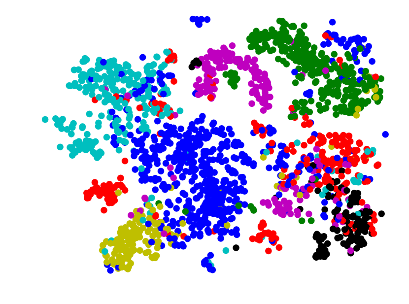
Depicted in Figure 1, our model for semi-supervised node classification builds on the GCN module proposed by Kipf and Welling (Kipf and Welling, 2017), which operates on the normalized adjacency matrix , as in , where , and is diagonal matrix of node degrees. Our proposed extension of GCNs is inspired by the recent advancements in random walk based graph embeddings (e.g. Perozzi et al., 2014; Grover and Leskovec, 2016; Abu-El-Haija et al., 2017). We make a Network of GCN modules (N-GCN), feeding each module a different power of , as in . The -th power contains statistics from the -th step of a random walk on the graph. Therefore, our N-GCN model is able to combine information from various step-sizes (i.e. graph scales). We then combine the output of all GCN modules into a classification sub-network, and we jointly train all GCN modules and the classification sub-network on the upstream objective for semi-supervised node classification. Weights of the classification sub-network give us insight on how the N-GCN model works. For instance, in the presence of input perturbations, we observe that the classification sub-network weights shift towards GCN modules utilizing higher powers of the adjacency matrix, effectively widening the “receptive field” of the (spectral) convolutional filters. We achieve state-of-the-art on several semi-supervised graph learning tasks, showing that explicit random walks enhance the representational power of vanilla GCN’s.
The rest of this paper is organized as follows. Section 2 reviews background work that provides the foundation for this paper. In Section 3, we describe our proposed method, followed by experimental evaluation in Section 4. We compare our work with recent closely-related methods in Section 5. Finally, we conclude with our contributions and future work in Section 6.
2. Background
2.1. Semi-Supervised Node Classification
Traditional label propagation algorithms (Weston et al., 2012; Belkin et al., 2006a) learn a model that transforms node features into node labels and uses the graph to add a regularizer term:
| (1) |
The first term trains the model to to predict the known labels . The second term is the graph-based regularizer, ensuring that connected nodes have a similar model output, with being the graph Laplacian and is the regularization coefficient hyperparameter.
2.2. Graph Convolutional Networks
Graph Convolution (Bruna et al., 2014) generalizes convolution from Euclidean domains to graph-structured data. Convolving a “filter” over a signal on graph nodes can be calculated by transforming both the filter and the signal to the Fourier domain, multiplying them, and then transforming the result back into the discrete domain. The signal transform is achieved by multiplying with the eigenvectors of the graph Laplacian. The transformation requires a quadratic eigendecomposition of the symmetric Laplacian; however, the low-rank approximation of the eigendecomposition can be calculated using truncated Chebyshev polynomials (Hammond et al., 2011). For instance, (Kipf and Welling, 2017) calculates a rank-1 approximation of the decomposition. They propose a multi-layer Graph Convolutional Networks (GCNs) for semi-supervised graph learning. Every layer computes the transformation:
| (2) |
where is the input activation matrix to the -th hidden layer with row containing a -dimensional feature vector for vertex , and is the layer’s trainable weights. The first hidden layer is set to the input features . A softmax on the last layer is used to classify labels. All layers use the same “normalized adjacency” , obtained by the “renormalization trick” utilized by (Kipf and Welling, 2017), as .111with added self-connections added as , similar to (Kipf and Welling, 2017)
Eq. (2) is a first order approximation of convolving filter over signal (Hammond et al., 2011; Kipf and Welling, 2017). The left-multiplication with averages node features with their direct neighbors; this signal is then passed through a non-linearity function (e.g, ReLU). Successive layers effectively diffuse signals from nodes to neighbors.
Two-layer GCN model can be defined in terms of vertex features and normalized adjacency as:
| (3) |
where the GCN parameters are trained to minimize the cross-entropy error over labeled examples. The output of the GCN model is a matrix , where is the number of nodes and is the number of labels. Each row contains the label scores for one node, assuming there are classes.
2.3. Graph Embeddings
Node Embedding methods represent graph nodes in a continuous vector space. They learn a dictionary , with one -dimensional embedding per node. Traditional methods use the adjacency matrix to learn embeddings. For example, Eigenmaps (Belkin and Niyogi, 2003) performs the following constrained optimization:
| (4) |
where is identity vector. Skipgram models on text corpora (Mikolov et al., 2013) inspired modern graph embedding methods, which simulate random walks to learn node embeddings (Perozzi et al., 2014; Grover and Leskovec, 2016). Each random walk generates a sequence of nodes. Sequences are converted to textual paragraphs, and are passed to a word2vec-style embedding learning algorithm (Mikolov et al., 2013). As shown in (Abu-El-Haija et al., 2017), this learning-by-simulation is equivalent, in expectation, to the decomposition of a random walk co-occurrence statistics matrix . The expectation on can be written as:
| (5) |
where is the row-normalized transition matrix (a.k.a right-stochastic adjacency matrix), and is a “context distribution” that is determined by random walk hyperparameters, such as the length of the random walk. The expectation therefore weights the importance of one node on another as a function of how well-connected they are, and the distance between them. The main difference between traditional node embedding methods and random walk methods is the optimization criteria: the former minimizes a loss on representing the adjacency matrix (see Eq. 4), while the latter minimizes a loss on representing random walk co-occurrence statistics .
3. Our Method
3.1. Motivation
Graph Convolutional Networks and random walk graph embeddings are individually powerful. (Kipf and Welling, 2017) uses GCNs for semi-supervised node classification. Instead of following traditional methods that use the graph for regularization (e.g. Eq. 4), (Kipf and Welling, 2017) use the adjacency matrix for training and inference, effectively diffusing information across edges at all GCN layers (see Eq. 3). Separately, recent work has showed that random walk statistics can be very powerful for learning an unsupervised representation of nodes that can preserve the structure of the graph (Perozzi et al., 2014; Grover and Leskovec, 2016; Abu-El-Haija et al., 2017).
Under special conditions, it is possible for the GCN model to learn random walks. In particular, consider a two-layer GCN defined in Eq. 3 with the assumption that first-layer activation is identity as , and weight is an identity matrix (either explicitly set or learned to satisfy the upstream objective). Under these two identity conditions, the model reduces to:
where can be expanded as:
| (6) |
By multiplying the adjacency with the transition matrix before, the is effectively doing a one-step random walk i.e. diffusing signals from nodes to neighbors, without non-linearities, then applying a non-linear Graph Conv layer.
3.2. Explicit Random Walks
The special conditions described above are not true in practice. Although stacking hidden GCN layers allows information to flow through graph edges, this flow is indirect as the information goes through feature reduction (matrix multiplication) and a non-linearity (activation function ). Therefore, the vanilla GCN cannot directly learn high powers of , and could struggle with modeling information across distant nodes. We hypothesize that making the GCN directly operate on random walk statistics will allow the network to better utilize information across distant nodes, in the same way that node embedding methods (e.g. DeepWalk, (Perozzi et al., 2014)) operating on are superior to traditional embedding methods operating on the adjacency matrix (e.g. Eigenmaps, (Belkin and Niyogi, 2003)). Therefore, in addition to feeding only to the GCN model as proposed by (Kipf and Welling, 2017) (see Eq. 3), we propose to feed a -degree polynomial of to instantiations of GCN. Generalizing Eq. (6) to arbitrary power gives:
| (7) |
We also define to be the identity matrix. Similar to (Kipf and Welling, 2017), we add self-connections and convert directed graphs to undirected ones, making and hence symmetric matrices. The eigendecomposition of symmetric matrices is real. Therefore, the low-rank approximation of the eigendecomposition (Hammond et al., 2011) is still valid, and a one layer of (Kipf and Welling, 2017) utilizing should still approximate multiplication in the Fourier domain.
3.3. Network of GCNs
Consider instantiations of , , , . Each GCN outputs a matrix , where the -th row describes a latent representation of that particular GCN for node , and is the latent dimensionality. Though can be different for each GCN, we set all to be the same for simplicity. We then combine the output of all GCN and feed them into a classification sub-network, allowing us to jointly train all GCNs and the classification sub-network via backpropagation. This should allow the classification sub-network to choose features from the various GCNs, effectively allowing the overall model to learn a combination of features using the raw (normalized) adjacency, different steps of random walks (i.e. graph scales), and the input features (as they are multiplied by identity ).
3.3.1. Fully-Connected Classification Network
From a deep learning prospective, it is intuitive to represent the classification network as a fully-connected layer. We can concatenate the output of the GCNs along the column dimension, i.e. concatenating all , each into matrix where . We add a fully-connected layer , with trainable parameter matrix , written as:
| (8) | ||||
| (10) |
The classifier parameters are jointly trained with GCN parameters . We use subscript fc on N-GCN to indicate the classification network is a fully-connected layer.
3.3.2. Attention Classification Network
We also propose a classification network based on “softmax attention”, which learns a convex combination of the GCN instantiations. Our attention model () is parametrized by vector , one scalar for each GCN. It can be written as:
| (11) |
where is output of a softmax: .
This softmax attention is similar to “Mixture of Experts” model, especially if we set the number of output channels for all GCNs equal to the number of classes, as in . This allows us to add cross entropy loss terms on all GCN outputs in addition to the loss applied at the output NGCN, forcing all GCN’s to be independently useful. It is possible to set the parameter vector “by hand” using the validation split, especially for reasonable such as . One possible choice might be setting to some small value and remaining to the harmonic series ; another choice may be linear decay . These are respectively similar to the context distributions of GloVe (Pennington et al., 2014) and word2vec (Mikolov et al., 2013; Levy et al., 2015). We note that if on average a node’s information is captured by its direct or nearby neighbors, then the output of GCNs consuming lower powers of should be weighted highly.
3.4. Training
We minimize the cross entropy between our model output and the known training labels as:
| (12) |
where is Hadamard product, and denotes a diagonal matrix, with entry at set to 1 if and 0 otherwise. In addition, we can apply intermediate supervision for the to attempt make all GCN become independently useful, yielding minimization objective:
| (13) |
3.5. GCN Replication Factor
3.6. Generalization to other Graph Models
In addition to vanilla GCNs (e.g. Kipf and Welling, 2017), our derivation also applies to other graph models including GraphSAGE (SAGE, Hamilton et al., 2017). Algorithm 1 shows a generalization that allows us to make a network of arbitrary graph models (e.g. GCN, SAGE, or others). Algorithms 2 and 3, respectively, show pseudo-code for the vanilla GCN (Kipf and Welling, 2017) and GraphSAGE222Our implementation assumes mean-pool aggregation by (Hamilton et al., 2017), which performs on-par to their top performer max-pool aggregation. In addition, our Algorithm 3 lists a full-batch implementation whereas (Hamilton et al., 2017) offer a mini-batch implementation. (Hamilton et al., 2017). Finally, Algorithm 4 defines our full Network of GCN model (N-GCN) by plugging Algorithm 2 into Algorithm 1. Similarly, Algorithm 5 defines our N-SAGE model by plugging Algorithm 3 in Algorithm 1.
We can recover the original algorithms GCN (Kipf and Welling, 2017) and SAGE (Hamilton et al., 2017), respectively, by using Algorithms 4 (N-GCN) and 5 (N-SAGE) with , , identity ClassifierFn, and modifying line 2 in Algorithm 1 to . Moreover, we can recover original DCNN (Atwood and Towsley, 2016) by calling Algorithm 4 with , , modifying line 3 to , and keeping as their proposed model operates on the power series of the transition matrix i.e. unmodified random walks, like ours.
4. Experiments
4.1. Datasets
We experiment on three citation graph datasets: Pubmed, Citeseer, Cora, and a biological graph: Protein-Protein Interactions (PPI). We choose the aforementioned datasets because they are available online and are used by our baselines. The citation datasets are prepared by (Yang et al., 2016), and the PPI dataset is prepared by (Hamilton et al., 2017). Table 1 summarizes dataset statistics.
Each node in the citation datasets represents an article published in the corresponding journal. An edge between two nodes represents a citation from one article to another, and a label represents the subject of the article. Each dataset contains a binary Bag-of-Words (BoW) feature vector for each node. The BoW are extracted from the article abstract. Therefore, the task is to predict the subject of articles, given the BoW of their abstract and the citations to other (possibly labeled) articles. Following (Yang et al., 2016) and (Kipf and Welling, 2017), we use 20 nodes per class for training, 500 (overall) nodes for validation, and 1000 nodes for evaluation. We note that the validation set is larger than training for these datasets!
4.2. Baseline Methods
For the citation datasets, we copy baseline numbers from (Kipf and Welling, 2017). These include label propagation (LP, (Zhu et al., 2003)); semi-supervised embedding (SemiEmb, (Weston et al., 2012)); manifold regularization (ManiReg, (Belkin et al., 2006b)); skip-gram graph embeddings (DeepWalk Perozzi et al., 2014); Iterative Classification Algorithm (ICA, Lu and Getoor, 2003); Planetoid (Yang et al., 2016); vanilla GCN (Kipf and Welling, 2017). For PPI, we copy baseline numbers from (Hamilton et al., 2017), which include GraphSAGE with LSTM aggregation (SAGE-LSTM) and GraphSAGE with pooling aggregation (SAGE). Further, for all datasets, we use our implementation to run baselines DCNN (Atwood and Towsley, 2016), GCN (Kipf and Welling, 2017), and SAGE (with pooling aggregation, Hamilton et al., 2017), as these baselines can be recovered as special cases of our algorithm, as explained in Section 3.6.
4.3. Implementation
We use TensorFlow(Abadi et al., 2015) to implement our methods, which we use to also measure the performance of baselines GCN, SAGE, and DCNN. For our methods and baselines, all GCN and SAGE modules that we train are 2 layers333except as clearly indicated in Table 4, where the first outputs 16 dimensions per node and the second outputs the number of classes (dataset-dependent). DCNN baseline has one layer and outputs 16 dimensions per node, and its channels (one per transition matrix power) are concatenated into a fully-connected layer that outputs the number of classes. We use dropout and L2 regularization of for all of the aforementioned models.
| Dataset | Type | Nodes | Edges | Classes | Features | Labeled nodes |
|---|---|---|---|---|---|---|
| Citeseer | citaction | 3,327 | 4,732 | 6 (single class) | 3,703 | 120 |
| Cora | citaction | 2,708 | 5,429 | 7 (single class) | 1,433 | 140 |
| Pubmed | citaction | 19,717 | 44,338 | 3 (single class) | 500 | 60 |
| PPI | biological | 56,944 | 818,716 | 121 (multi-class) | 50 | 44,906 |
| Method | Citeseer | Cora | Pubmed | PPI | |
| (a) | ManiReg (Belkin et al., 2006b) | – | |||
| (b) | SemiEmb (Weston et al., 2012) | – | |||
| (c) | LP (Zhu et al., 2003) | – | |||
| (d) | DeepWalk (Perozzi et al., 2014) | – | |||
| (e) | ICA (Lu and Getoor, 2003) | – | |||
| (f) | Planetoid (Yang et al., 2016) | – | |||
| (g) | GCN (Kipf and Welling, 2017) | – | |||
| (h) | SAGE-LSTM (Hamilton et al., 2017) | – | – | – | |
| (i) | SAGE (Hamilton et al., 2017) | – | – | – | |
| (j) | DCNN (our implementation) | ||||
| (k) | GCN (our implementation) | ||||
| (l) | SAGE (our implementation) | ||||
| (m) | N-GCN (ours) | ||||
| (n) | N-SAGE (ours) |
| Nodes per class | 5 | 10 | 20 | 100 |
|---|---|---|---|---|
| DCNN (our implementation) | ||||
| GCN (our implementation) | ||||
| SAGE (our implementation) | ||||
| (ours) | ||||
| (ours) | ||||
| (ours) | ||||
| (ours) |


4.4. Node Classification Accuracy
Table 2 shows node classification accuracy results. We run 20 different random initializations for every model (baselines and ours), train using Adam optimizer (Ba and Kingma, 2015) with learning rate of 0.01 for 600 steps, capturing the model parameters at peak validation accuracy to avoid overfitting. For our models, we sweep our hyperparameters , , and choice of classification sub-network . For baselines and our models, we choose the model with the highest accuracy on validation set, and use it to record metrics on the test set in Table 2.
4.5. Sensitivity Analysis
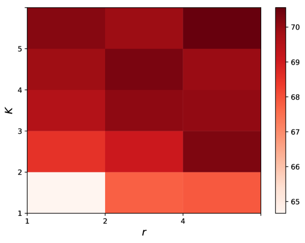
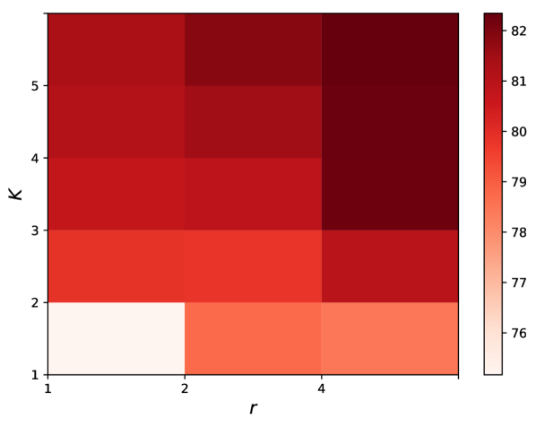
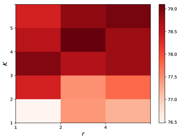
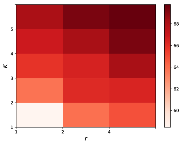
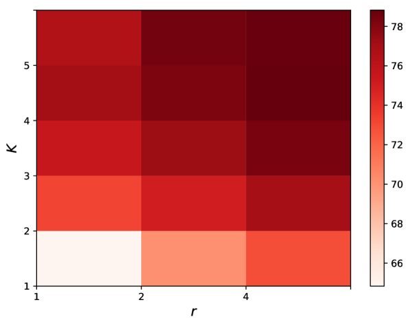
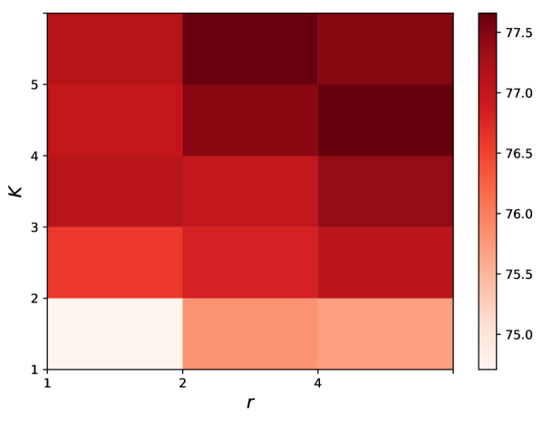
We analyze the impact of random walk length and replication factor on classification accuracy in Figure 2. In general, model performance improves when increasing and . We note utilizing random walks by setting improves model accuracy due to the additional information, not due to increased model capacity: Contrast (i.e. mixture of GCNs, no random walks) with (i.e. N-GCN on random walks) – in both scenarios, the model has more capacity, but the latter shows better performance. The same holds for SAGE.
4.6. Tolerance to feature noise
We test our method under feature noise perturbations by removing node features at random. This is practical, as article authors might forget to include relevant terms in the article abstract, and more generally not all nodes will have the same amount of detailed information. Figure 3 shows that when features are removed, methods utilizing unmodified random walks: N-GCN, N-SAGE, and DCNN, outperform convolutional methods including GCN and SAGE. Moreover, the performance gap widens as we remove more features. This suggests that our methods can somewhat recover removed features by directly pulling-in features from nearby and distant neighbors. We visualize in Figure 4 the attention weights as a function of % features removed. With little feature removal, there is some weight on , and the attention weights for follow some decay function. Maliciously dropping features causes our model to shift its attention weights towards higher powers of .
4.7. Random Walk Steps Versus GCN Depth
-step random walk will allow every node to accumulate information from its neighbors, up to distance . Similarly, a -layer GCN (Kipf and Welling, 2017) will do the same. The difference between the two was mathematically explained in Section 3.1. To summarize: the former averages node feature vectors according to the random walk co-visit statistics, whereas the latter creates non-linearities and matrix multiplies at every step. So far, we displayed experiments where our models (N-GCN and N-SAGE) were able to use information from distant nodes (e.g. ), but for all GCN and SAGE modules, we used 2 GCN layer for baselines and our models.
Even though the authors of GCN (Kipf and Welling, 2017) and SAGE (Hamilton et al., 2017) suggest using two GCN layers, according by holdout validation, for a fair comparison with our models, we run experiments utilizing deeper GCN and SAGE are models so that its “receptive field” is comparable to ours.
| Graph Conv Layer Dimensions | ||||
|---|---|---|---|---|
| Dataset | Model | |||
| Citeseer | GCN | 0.699 | 0.632 | 0.659 |
| Citeseer | SAGE | 0.668 | 0.660 | 0.674 |
| Cora | GCN | 0.803 | 0.800 | 0.780 |
| Cora | SAGE | 0.761 | 0.763 | 0.757 |
| Pubmed | GCN | 0.762 | 0.771 | 0.781 |
| Pubmed | SAGE | 0.770 | 0.776 | 0.775 |
| PPI | GCN | 0.460 | 0.461 | 0.466 |
| PPI | SAGE | 0.658 | 0.672 | 0.650 |
Table 4 shows test accuracies when training deeper GCN and SAGE models, using our implementation. We notice that, unlike our method which benefits from a wider “receptive field”, there is no direct correspondence between depth and improved performance.
5. Related Work
The field of graph learning algorithms is quickly evolving. We review work most similar to ours.
Defferrard et al (Defferrard et al., 2016) define graph convolutions as a -degree polynomial of the Laplacian, where the polynomial coefficients are learned. In their setup, the -th degree Laplacian is a sparse square matrix where entry at will be zero if nodes and are more than hops apart. Their sparsity analysis also applies here. A minor difference is the adjacency normalization. We use whereas they use the Laplacian defined as . Raising to power will produce a square matrix with entry being the probability of random walker ending at node after steps from node . The major difference is the order of random walk versus non-linearity. In particular, their model calculates learns a linear combination of -degree polynomial and pass through classifier function , as in , while our (e.g. N-GCN) model calculates , where is in our model and in theirs, and our can be a GCN module. In fact, (Defferrard et al., 2016) is also similar to work by (Abu-El-Haija et al., 2017), as they both learn polynomial coefficients to some normalized adjacency matrix.
Atwood and Towsley (Atwood and Towsley, 2016) propose DCNN, which calculates powers of the transition matrix and keeps each power in a separate channel until the classification sub-network at the end. Their model is therefore similar to our work in that it also falls under . However, where their model multiplies features with each power once, our model makes use of GCN’s (Kipf and Welling, 2017) that multiply by at every GCN layer (see Eq. 2). Thus, DCNN model (Atwood and Towsley, 2016) is a special case of ours, when GCN module contains only one layer, as explained in Section 3.6.
6. Conclusions and Future Work
In this paper, we propose a meta-model that can run arbitrary Graph Convolution models, such as GCN (Kipf and Welling, 2017) and SAGE (Hamilton et al., 2017), on the output of random walks. Traditional Graph Convolution models operate on the normalized adjacency matrix. We make multiple instantiations of such models, feeding each instantiation a power of the adjacency matrix, and then concatenating the output of all instances into a classification sub-network. Each instantiation is therefore operating on different scale of the graph. Our model, Network of GCNs (and similarly, Network of SAGE), is end-to-end trainable, and is able to directly learn information across near or distant neighbors. We inspect the distribution of parameter weights in our classification sub-network, which reveal to us that our model is effectively able to circumvent adversarial perturbations on the input by shifting weights towards model instances consuming higher powers of the adjacency matrix. For future work, we plan to extend our methods to a stochastic implementation and tackle other (larger) graph datasets.
References
- (1)
- Abadi et al. (2015) Martín Abadi, Ashish Agarwal, Paul Barham, Eugene Brevdo, Zhifeng Chen, Craig Citro, Greg S. Corrado, Andy Davis, Jeffrey Dean, Matthieu Devin, Sanjay Ghemawat, Ian Goodfellow, Andrew Harp, Geoffrey Irving, Michael Isard, Yangqing Jia, Rafal Jozefowicz, Lukasz Kaiser, Manjunath Kudlur, Josh Levenberg, Dan Mané, Rajat Monga, Sherry Moore, Derek Murray, Chris Olah, Mike Schuster, Jonathon Shlens, Benoit Steiner, Ilya Sutskever, Kunal Talwar, Paul Tucker, Vincent Vanhoucke, Vijay Vasudevan, Fernanda Viégas, Oriol Vinyals, Pete Warden, Martin Wattenberg, Martin Wicke, Yuan Yu, and Xiaoqiang Zheng. 2015. TensorFlow: Large-Scale Machine Learning on Heterogeneous Systems. https://www.tensorflow.org/
- Abu-El-Haija et al. (2017) Sami Abu-El-Haija, Bryan Perozzi, Rami Al-Rfou, and Alex Alemi. 2017. Watch Your Step: Learning Graph Embeddings Through Attention. In arxiv.
- Atwood and Towsley (2016) James Atwood and Don Towsley. 2016. Diffusion-Convolutional Neural Networks. In Advances in Neural Information Processing Systems (NIPS).
- Ba and Kingma (2015) Jimmy Ba and Diederik Kingma. 2015. Adam: A Method for Stochastic Optimization. In International Conference on Learning Representations.
- Belkin and Niyogi (2003) Mikhail Belkin and Partha Niyogi. 2003. Laplacian Eigenmaps for Dimensionality Reduction and Data Representation. In Neural Computation.
- Belkin et al. (2006a) Mikhail Belkin, Partha Niyogi, and Vikas Sindhwani. 2006a. Manifold regularization: A geometric framework for learning from labeled and unlabeled examples. In Journal of machine learning research (JMLR).
- Belkin et al. (2006b) Mikhail Belkin, Partha Niyogi, and Vikas Sindhwani. 2006b. Manifold regularization: A geometric framework for learning from labeled and unlabeled examples. In Journal of machine learning research (JMLR).
- Bruna et al. (2014) J. Bruna, W. Zaremba, A. Szlam, and Y. LeCun. 2014. Spectral Networks and Locally Connected Networks on Graphs. In International Conference on Learning Representations.
- Defferrard et al. (2016) Michaël Defferrard, Xavier Bresson, and Pierre Vandergheynst. 2016. Convolutional Neural Networks on Graphs with Fast Localized Spectral Filtering. In Advances in Neural Information Processing Systems (NIPS).
- Grover and Leskovec (2016) A. Grover and J. Leskovec. 2016. node2vec: Scalable Feature Learning for Networks. In Proceedings of the 22nd ACM SIGKDD International Conference on Knowledge Discovery and Data Mining.
- Hamilton et al. (2017) W. Hamilton, R. Ying, and J. Leskovec. 2017. Inductive Representation Learning on Large Graphs. In NIPS.
- Hammond et al. (2011) David K. Hammond, Pierre Vandergheynst, and R. Gribonval. 2011. Wavelets on graphs via spectral graph theory. In Applied and Computational Harmonic Analysis.
- He et al. (2016) Kaiming He, Xiangyu Zhang, Shaoqing Ren, and Jian Sun. 2016. Deep Residual Learning for Image Recognition. In IEEE Conference on Computer Vision and Pattern Recognition (CVPR).
- Kipf and Welling (2017) T. Kipf and M. Welling. 2017. Semi-Supervised Classification with Graph Convolutional Networks. In International Conference on Learning Representations.
- Krizhevsky et al. (2012) Alex Krizhevsky, Ilya Sutskever, and Geoffrey E Hinton. 2012. ImageNet Classification with Deep Convolutional Neural Networks. In Advances in Neural Information Processing Systems.
- LeCun et al. (1998) Y. LeCun, L. Bottou, Y. Bengio, and P. Haffner. 1998. Gradient-based learning applied to document recognition. In Proceedings of the IEEE.
- Levy et al. (2015) Omer Levy, Yoav Goldberg, and Ido Dagan. 2015. Improving Distributional Similarity with Lessons Learned from Word Embeddings. In Transactions of the Association for Computational Linguistics (TACL).
- Lu and Getoor (2003) Qing Lu and Lise Getoor. 2003. Link-based classification. In International Conference on Machine Learning (ICML).
- Merdan et al. (2017) Selin Merdan, Christine L. Barnett, and Brian T. Denton. 2017. Data Analytics for Optimal Detection of Metastatic Prostate Cancer. (2017).
- Mikolov et al. (2013) T. Mikolov, I. Sutskever, K. Chen, G. Corrado, and J. Dean. 2013. Distributed representations of words and phrases and their compositionality. In Advances in Neural Information Processing Systems.
- Pennington et al. (2014) Jeffrey Pennington, Richard Socher, and Christopher D. Manning. 2014. Glove: Global Vectors for Word Representation. In Conference on Empirical Methods in Natural Language Processing, EMNLP.
- Perozzi et al. (2014) B. Perozzi, R. Al-Rfou, and S. Skiena. 2014. DeepWalk: Online Learning of Social Representations. In Knowledge Discovery and Data Mining.
- Szegedy et al. (2015) Christian Szegedy, Wei Liu, Yangqing Jia, Pierre Sermanet, Scott E. Reed, Dragomir Anguelov, Dumitru Erhan, Vincent Vanhoucke, and Andrew Rabinovich. 2015. Going Deeper with Convolutions. In IEEE Conference on Computer Vision and Pattern Recognition (CVPR).
- Weston et al. (2012) Jason Weston, Frederic Ratle, Hossein Mobahi, and Ronan Collobert. 2012. Deeplearning via semi-supervised embedding. In Neural Networks: Tricks of the Trade. 639–655.
- Yang et al. (2016) Z. Yang, W. Cohen, and R. Salakhutdinov. 2016. Revisiting Semi-Supervised Learning with Graph Embeddings. In International Conference on Machine Learning (ICML).
- Zhu et al. (2003) Xiaojin Zhu, Zoubin Ghahramani, and John Lafferty. 2003. Semi-supervised learning using gaussian fields and harmonic functions. In International Conference on Machine Learning (ICML).