Classifying surface probe images in strongly correlated electronic systems via machine learning

Abstract

Scanning probe experiments such as scanning tunneling microscopy (STM) and atomic force microscopy (AFM) on strongly correlated electronic systems often reveal complex pattern formation on multiple length scales.Qazilbash et al. (2007); Kohsaka et al. (2007) By studying the universal scaling in these images, we have shown in several distinct correlated electronic systems that the pattern formation is driven by proximity to a disorder-driven critical point,Phillabaum et al. (2012); Liu et al. (2016) revealing a unification of the pattern formation in these materials. As an alternative approach to this image classification problem of novel materials, here we report the first investigation of the machine learning method to determine which underlying physical model is driving pattern formation in a system. Using a neural network architecture, we are able to achieve 97$\%$ accuracy on classifying configuration images from three models with Ising symmetry. This investigation also demonstrates that machine learning can capture the implicit universal behavior of a physical system. This broadens our understanding of what machine learning can do, and we expect more synergy between machine learning and condensed matter physics in the future.

I Introduction

Scanning probe experiments often reveal complex pattern formation at the surface of strongly correlated electronic systemsQazilbash et al. (2007); Kohsaka et al. (2007); Phillabaum et al. (2012); Liu et al. (2016); Dagotto (2005); Moreo et al. (2000). Since their invention in 1982, scanning probes have revolutionized our understanding of materials, yielding an ever increasing wealth of data on a wide variety of materialsBinnig and Rohrer (2013). To date, the majority of theoretical treatments have focused on microscopic physics Bonnell et al. (2012), with few theoretical treatments offering guidance for how to interpret the detailed spatial information available in the emergent multiscale pattern formation often observed on surfaces. For systems near criticality, the spatial configurations of geometric clusters become scale-free, displaying spatial complexity on multiple length scales in a way that is controlled by the critical fixed point. Therefore, the geometric properties encode critical exponents, as we have shown elsewhere.Phillabaum et al. (2012); Carlson et al. (2015); Liu et al. (2016) Such scale-free complexity can arise from interactions deep within a material, or from surface-only physics, or even from a non-interacting model at the right concentration. We show here that artificial neural networks can be trained to identify which physics is responsible for the complex pattern formation, identifying whether interactions are present, and if so, whether the interactions arise from deep inside the material, or whether they arise from surface physics.

Machine learning (ML) is a burgeoning field in computer science and data science, with broad applications across disciplines such as bioinformatics, computer vision, marketing, economics, and medical diagnosis. A computer program is said to exhibit ML if its ability to perform a given task increases with experience, as determined by some performance metric. That is, the program accumulates iterative modifications when presented with certain input (“experience”), in such a way as to improve its performance at the task, without those modifications being explicitly programmed.Russell and Norvig (2015)

In physics, ML has been applied to to physics at a range of scales, from galaxy clustersBall and Brunner (2010) to elementary particlesWhiteson and Whiteson (2009). ML is beginning to be applied in condensed matter physics, for example in quantum many body problemsCarleo and Troyer (2017), electronic quantum transportLopez-Bezanilla and von Lilienfeld (2014), glassy dynamicsSchoenholz et al. (2016), phase transitionsWang (2016); Carrasquilla and Melko (2016), renormalization groupMehta and Schwab (2014); Beny (2013), and big data issues of materials scienceKusne et al. (2014); Ghiringhelli et al. (2015); Kalinin et al. (2015). Arsenault et al. have used ML to address problems in many-body physics such as the Anderson impurity modelArsenault et al. (2014) and dynamical mean-field theory.Arsenault et al. (2015). Carleo and Troyer used ML to study the wavefunction of quantum many-body interacting spin systems.Carleo and Troyer (2017) Wang showed that an unsupervised learning algorithm could “discover” that the order parameter and structure factor change significantly as the temperature is varied through the phase transition.Wang (2016) Carrasquilla and Melko have shown that for a few different models, supervised learning can distinguish the ordered from the disordered phase.Carrasquilla and Melko (2016)

However, no one has yet tasked ML with identifying which underlying Hamiltonian is actually responsible for the phase transition. We show in this paper that ML can be used to identify which model was used to generate a particular spin configuration, focusing on configurations that are close to criticality. We focus on near-critical configurations, since these are most relevant to interpreting the multiscale pattern formation observed in many spatially resolved experiments.Qazilbash et al. (2007); Kohsaka et al. (2007); Phillabaum et al. (2012); Liu et al. (2016); Dagotto (2005); Moreo et al. (2000) This type of identification can reveal information such as which interactions are important, whether quenched disorder is a relevant term in the Hamiltonian, and how many dimensions are involved in the phenomenon (to determine, for example, whether observed patterns in data are driven by surface physics, or from the bulk of the material).

In this paper, we are interested in whether ML can classify microscopy images according to the underlying physics driving the complex pattern formation. To be more specific, we want to know whether ML can capture the universal properties and critical behavior implied by the image patterns, and then identify which model generated the image. In the present work we limit ourselves to three theoretical models: the two-dimensional (2D) clean Ising model on a square lattice (Fig. 1); the three-dimensional (3D) clean Ising model on a cubic lattice (Fig. 2); and the square lattice site percolation model (Fig. 3). The Ising models may be written as:

$$H=-J\sum_{<ij>}\sigma_{i}\sigma_{j}$$ (1)

where $\sigma_{i}=\pm 1$ and $J$ is the coupling strength between nearest neighbor sites, and the summation runs over the sites of either a two-dimensional square lattice or a three-dimensional cubic lattice.

Ising models were first used to describe magnetic transitions, from a ferromagnetically ordered phase at low temperature $T<T_{c}$, to a paramagnetic, disordered phase above the magnetic ordering temperature $T_{c}$,Fisher (1974); Stanley (1971) in systems where magnetic moments are constrained to point either “up” or “down.” However, the model can be applied to a wide variety of physical systems. For example, the behavior of the critical endpoint of the liquid-gas phase transition is well described by the criticality of the three-dimensional Ising model. Electrons inside of solids have their own phase transitions, and when comparing to experiments on these systems, $\sigma$ may be viewed as a generalized pseudospin in the context of two-component electronic behavior. This may be mapped, for example, to the two perpendicular orientations of nematic stripes in cuprate superconductors,Phillabaum et al. (2012) or to the metal and insulator islands in VO₂.Liu et al. (2016)

In the absence of interactions, pseudospins may be said to follow a percolation model, which is a non-interacting model. Therefore we also consider site percolation on a square lattice, assigning a probability $p$ to having pseudospin $\sigma=1$ on any given site, otherwise the pseudospin is assigned as $\sigma=-1$. In two dimensions, this model has a continuous phase transition (and therefore exhibits criticality) at $p_{c}=0.59$. We aim to explore the efficiency of ML for capturing features associated with the corresponding universality class, including interactions, disorder, and dimension. Other universal features, such as the type of random disorder in the system, and the symmetry of the order parameter, are left for future work.

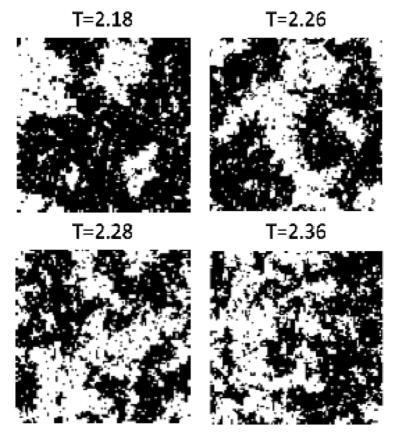
Figure 1: Ising 2D images. Row 1: $T\textless T_{c}$, row 2: $T\approx T_{c}=2.269$, row 3: $T\textgreater T_{c}$. Temperatures are in units of J, which is the coupling strength between Ising variables. Black and white pixels represent Ising variables $\sigma=+1$ and $-1$ respectively.

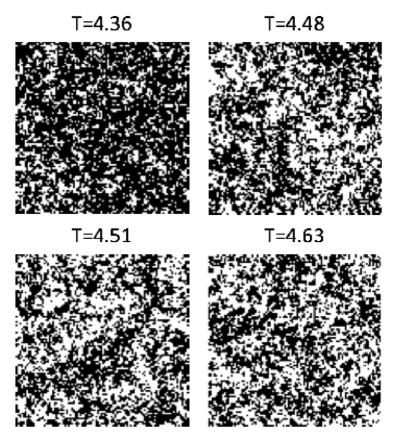
Figure 2: Ising 3D images. Row 1: $T\textless T_{c}$, row 2: $T\approx T_{c}=4.512$, row 3: $T\textgreater T_{c}$. Temperatures are in units of J, which is the coupling strength between Ising variables. Black and white pixels represent Ising variables $\sigma=+1$ and $-1$ respectively.

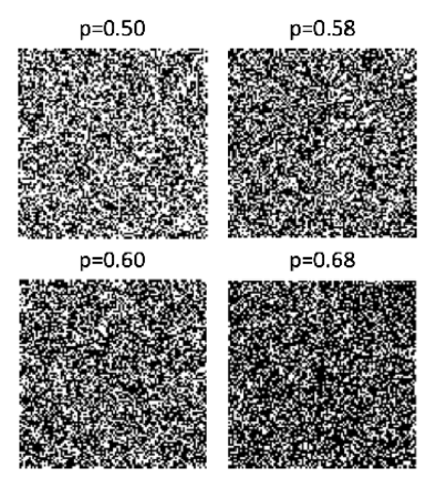
Figure 3: Percolation images. Row 1: $p\textless p_{c}$, row 2: $p\approx p_{c}$, row 3: $p\textgreater p_{c}$. On a square lattice, the site percolation threshold is $p_{c}=0.59$. Black and white pixels represent variables $\sigma=+1$ and $-1$ respectively.

II Methods

With ML, a software program undergoes significant changes based on new input, without those changes being explicitly hard-coded by the programmer. Rather, training algorithms contained within the program train the neural network as new input is received.Russell and Norvig (2015) Whereas human visual pattern classification and recognition can be viewed as a qualitative process, ML turns this into an explicitly quantitative process, albeit within some margin of error. In our case, we have used a scaled conjugate gradient (SCG) algorithmMoller (1993) under supervised learning conditions to train a neural network algorithm using the MATLAB Neural Network Toolbox through XSEDETowns et al. (2014). With supervised learning, the program is presented with a training set of data for which the “right answer” is also supplied to the training algorithm. The point is to develop an algorithm that gives the correct output for a given input. In our case, the goal will be to identify the underlying interacting physics model (the output) from which a particular Ising spin configuration was generated (the input).

In order to accomplish this, we have used an artificial neural network with a single hidden layer containing 200 “neurons”. Each neuron consists of multiple inputs, a nonlinear activation function, and a single output. We use a hyperbolic tangent activation function, which results in outputs between -1 and 1. The network is defined by its topology (how the neurons are interconnected) and the weights associated with each connection. We use a feedforward neural network, which can be represented by a directed acyclic graph where each edge has a weight and each node has a bias. A very small example of a neural network topology is illustrated in Fig. 4. The input layer consists of the black and white image itself, where each circle represents one pixel. In the hidden layer, each circle represents a single neuron, with multiple inputs, which turns on according to some nonlinear function of its input weights. The output layer in our case has three nodes, one for each of the three models which may generate a spatially complex image near criticality.

The goal of neural network training is to optimize the weights and biases of the network, by minimizing a loss function. In the present case, we use cross entropy as the loss function. The training proceeds towards a point where the loss function is at a minimum. We have used scaled conjugate gradient descent methodMoller (1993) to minimize the loss function. We furthermore use backpropagation of errors, a type of automatic differentiation in which the derivatives associated with the chain rule are computed in reverse order (i.e. working from the topmost dependent variable down through to the independent variables).

Neurons	50	75	100	125	150	200	250
% Accuracy	94.93	95.53	95.95	96.48	96.68	97.00	96.72

Table 1: Classification accuracy for a given number of hidden neurons. Accuracy initially increases with increasing number of hidden neurons.

We use the 2D percolation model and Monte Carlo simulations of the 2D clean Ising model and 3D clean Ising model to generate images to train the neural network. For the 2D models, the neural network is directly fed spin configurations near criticality for training purposes. For the 3D model, the neural network is fed spin configurations from a 2D slice of the 3D lattice. This is to mimic surface probe experiments, which have access to only 2D information. The goal is for the neural network to learn to identify which model generated which images.

The “interesting” cases occur near criticality, where geometric clusters (as defined by connected sets of like-spin nearest neighbors) grow in such a way as to have structure over multiple length scales. Near criticality, systems experience fluctuations over all length scales from atomic to the size of the system. Because there is no characteristic length scale in between, critical systems are described by power law behavior, where the exponent of each power law is called a “critical exponent.” At any second order phase transition, the unique set of critical exponents acts like a fingerprint to identify the universality class of the phase transition, which is set by universal features such as the dimension of the lattice and the symmetry of the order parameter ($Z_{2}$ in the case of Ising variables $\sigma=\pm 1$), and independent of “non-universal” short-distance physics like the inclusion of 2nd-nearest-neighbor interactions.Fisher (1974); Stanley (1971) Ultimately, this behavior arises because the geometric clusters have a fractal character near criticality, whereby each cluster is scale-free. In these cases, we have shownPhillabaum et al. (2012); Carlson et al. (2015); Liu et al. (2016) that the statistics of the shapes of the clusters in the images encodes the universality class of the underlying model. The hardest cases to judge by eye are those with roughly equal numbers of up and down spins. For this reason, we focus attention within 4% of the critical region of the Ising models (since magnetization rapidly develops inside the ordered region), and within 15% of the percolation model (because equal numbers of up and down spins in that case is p=0.5, which is close but not at the critical value of $p_{c}=0.59$ for site percolation on a square lattice). Note that net magnetization is not a trivial discriminator of these models near criticality. Within these parameter ranges, each model covers states with no net magnetization as well as those with net magnetization in the thermodynamic (infinite size) limit. Even more importantly, for the same nominal set of model parameters, thermal fluctuations can cause a net magnetization to appear in a finite size system for $T>T_{c}$. It is especially important to distinguish whether interactions are present, in order to determine in any given surface probe experiment whether interactions are responsible for the observed pattern formation, in order to distinguish it from putative “dirt effects” which may arise at the surface of a material. Because the Ising models are near criticality, we use the Wolff algorithm, and sample spin configurations every 100 Monte Carlo steps to ensure independent sampling. We simulate system sizes of $L^{2}=100^{2}$ for the 2D case, and $L^{3}=100^{3}$ for the 3D case. (For comparison, experimental images from surface probes in condensed matter physics today are typically about $200\times 200$ pixels.Bonnell et al. (2012)) The images passed to the neural network consist of $100\times 100=10,000$ pixels, called “features” in the context of ML; the number of training examples given to the neural network must be significantly greater than We use 400,000 configurations from each model, for a total of 1,200,000 configurations. These configurations are then divided randomly, using 70% for training, 15% for validation, and 15% for testing.

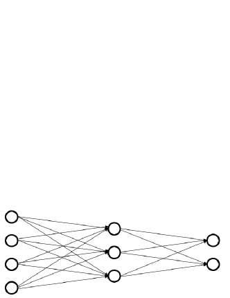
Figure 4: Schematic of a small artificial neural network. In this case there are 4 features in the input data (for example pixels in a 2x2 image), 3 hidden neurons, and 2 outputs (for example cat/dog, or percolation/Ising).

III Results and Discussion

We find that the neural network, once trained to identify which model produced which spin configurations, achieves an average classification accuracy of about 97%, once the number of hidden neurons is at least 150. The dependence of the classification accuracyon the number of hidden neurons is shown in Table 1. The error bars are calculated from the case with 200 neurons where multiple training runs where conducted. The classification error drops from around 5$\%$ at 50 neurons to around 3$\%$ at 150 neurons. Results between 150 and 250 neurons are very similar and adding more neurons than 150 does not help much, although there does appear to be a minimum in the error for 200 neurons.

The case study presented in Table 2 shows how errors were distributed among the models. The rows represent the models that images belong to and columns represent the models that images were classified as. The most misclassified model is the 3D Ising model. It was particularly hard for the neural network to distinguish between the 2D and 3D Ising models. Ising 2D and percolation are the most easily distinguished with almost negligible errors.

We have shown that ML can be used to classify configuration images into their associated universality classes, which means that it identifies implicit universal properties underlying the complex pattern formation of image configurations near a critical point. The conventional approach to identifying a universality class is to first explicitly fit the experimental data in order to find the critical exponents, then match that set of critical exponents to a known universality class. However, the approach developed here does not depend upon critical exponents. Instead, we feed image data and universality class labels to the machine learning model and let the ML algorithm develop its own internal parameters in the neural network. We haven’t programmed the model to include any theories from physics, but the model learns directly from the data, and then captures the universal features in the configuration images to identify the universality class. Thus, we have shown that it is possible to go directly from data to an identification of the universality class of that data, without explicitly considering any critical exponents or scaling theory.

This finding broadens our understanding of the extent to which ML can be applied, and thus has important implications in the field of ML and computer vision where the image classification problem is mainly focused on explicit object recognition, rather than discovering underlying physics. We also expect that machine learning can be used to study and even learn more complex physics given large enough datasets. This synergy between machine learning and physics opens a new perspective for future research in condensed matter physics, or even in all fields of physics, that we can draw important conclusions via ML, without the need to interpret the intermediate steps of the ML algorithm.

		Neural network output
		perc	I-2D	I-3D
Input model	perc	98.05%	0.01%	1.94%
	I-2D	0.03%	98.30%	1.67%
	I-3D	1.82%	2.96%	95.22%

Table 2: Classfication results for testing data for the case of 200 neurons in the hidden layer. The model listed on each row denotes the Hamiltonian used to generate spin configurations to present to the neural network. In each column, the output of the neural network is listed. The goal is to train the neural network to identify which model produced which spin configurations.

IV Conclusion

In conclusion, we have shown that machine learning can successfully determine which spin configurations were generated from which theoretical model when the images are near criticality. As scanning probe experimental capabilities grow, they are producing a growing wealth of data, including more examples of systems in which the electronic textures display multiscale pattern formation at the surface of the material.Qazilbash et al. (2007); Kohsaka et al. (2007); Lupi et al. (2010); Battisti et al. (2016) In cases where the pattern formation is driven by proximity to a critical point,Phillabaum et al. (2012); Carlson et al. (2015); Liu et al. (2016) the techniques employed here can be used to identify the underlying physics driving the pattern formation, without the need to explicitly determine critical exponents or scaling forms.

V Acknowledgements

LB acknowledges support from the SURF program through the College of Engineering at Purdue University. SL acknowledges support from the Bilsland Dissertation Fellowship at Purdue University. EWC and SL acknowledge support from NSF DMR-1508236 and Dept. of Education Grant No. P116F140459. This work used the Extreme Science and Engineering Discovery Environment (XSEDE), which is supported by National Science Foundation grant number ACI-1053575.

References

- Qazilbash et al. (2007) M. M. Qazilbash, M. Brehm, B.-G. Chae, P.-C. Ho, G. O. Andreev, B.-J. Kim, S. J. Yun, A. V. Balatsky, M. B. Maple, F. Keilmann, H.-T. Kim, and D. N. Basov, Science 318, 1750 (2007).
- Kohsaka et al. (2007) Y. Kohsaka, C. Taylor, K. Fujita, A. Schmidt, C. Lupien, T. Hanaguri, M. Azuma, M. Takano, H. Eisaki, H. Takagi, S. Uchida, and J. C. Davis, Science 315, 1380 (2007).
- Phillabaum et al. (2012) B. Phillabaum, E. W. Carlson, and K. A. Dahmen, Nat. Commun. 3, 915 (2012).
- Liu et al. (2016) S. Liu, B. Phillabaum, E. W. Carlson, K. A. Dahmen, N. S. Vidhyadhiraja, M. M. Qazilbash, and D. N. Basov, Phys. Rev. Lett. 116, 036401 (2016).
- Dagotto (2005) E. Dagotto, Science 309, 257 (2005).
- Moreo et al. (2000) A. Moreo, M. Mayr, A. Feiguin, S. Yunoki, and E. Dagotto, Phys. Rev. Lett. 84, 5568 (2000).
- Binnig and Rohrer (2013) G. Binnig and H. Rohrer, Reviews of Modern Physics 71, 324 (2013).
- Bonnell et al. (2012) D. A. Bonnell, D. N. Basov, M. Bode, U. Diebold, S. V. Kalinin, V. Madhavan, L. Novotny, M. Salmeron, U. D. Schwarz, and P. S. Weiss, Reviews of Modern Physics 84, 1343 (2012).
- Carlson et al. (2015) E. W. Carlson, S. Liu, B. Phillabaum, and K. A. Dahmen, Journal of Superconductivity and Novel Magnetism (2015).
- Russell and Norvig (2015) S. Russell and P. Norvig, “Artificial intelligence: A modern approach,” (Pearson, 2015) Chap. V.
- Ball and Brunner (2010) N. Ball and R. Brunner, Int. Journal of Modern Physics D 19, 1049 (2010).
- Whiteson and Whiteson (2009) S. Whiteson and D. Whiteson, Engineering Applications of AI 22, 1203 (2009).
- Carleo and Troyer (2017) G. Carleo and M. Troyer, Science 355, 602 (2017), arXiv:1606.02318.
- Lopez-Bezanilla and von Lilienfeld (2014) A. Lopez-Bezanilla and O. von Lilienfeld, Phys. Rev. B 89 (2014).
- Schoenholz et al. (2016) S. Schoenholz, E. Cubuk, D. Sussman, and et al., Nature Physics 12 (2016).
- Wang (2016) L. Wang, “Discovering phase transitions with unsupervised learning,” (2016), arXiv: 1606.00318.
- Carrasquilla and Melko (2016) J. Carrasquilla and R. Melko, “Machine learning phases of matter,” (2016), arXiv: 1605.01735.
- Mehta and Schwab (2014) P. Mehta and D. Schwab, “An exact mapping between the variational renormalization group and deep learning,” (2014), arXiv: 1410.3831.
- Beny (2013) C. Beny, “Deep learning and the renormalization group,” (2013), arXiv: 1301.3124.
- Kusne et al. (2014) A. Kusne, T. Gao, A. Mehta, and et al., Scientific Reports 4 (2014).
- Ghiringhelli et al. (2015) L. M. Ghiringhelli, J. Vybiral, S. V. Levchenko, C. Draxl, and M. Scheffler, Phys. Rev. Lett. 114, 105503 (2015).
- Kalinin et al. (2015) S. Kalinin, B. Sumpter, and R. Archibald, Nature Materials 14 (2015).
- Arsenault et al. (2014) L.-F. Arsenault, A. Lopez-Bezanilla, O. A. von Lilienfeld, and A. J. Millis, Phys. Rev. B 90, 155136 (2014).
- Arsenault et al. (2015) L.-F. Arsenault, O. A. von Lilienfeld, and A. J. Millis, “Machine learning for many-body physics: efficient solution of dynamical mean-field theory,” (2015), arXiv:1506.08858.
- Fisher (1974) M. E. Fisher, Rev. Mod. Phys. 46, 597 (1974).
- Stanley (1971) H. E. Stanley, Introduction to Phase Transitions and Critical Phenomena (Oxford University Press, 1971).
- Moller (1993) M. F. Moller, Neural Networks 6, 525 (1993).
- Towns et al. (2014) J. Towns, T. Cockerill, M. Dahan, I. Foster, K. Gaither, A. Grimshaw, V. Hazlewood, S. Lathrop, D. Lifka, G. D. Peterson, R. Roskies, J. R. Scott, and N. Wilkins-Diehr, Computing in Science and Engineering 16, 62 (2014).
- Lupi et al. (2010) S. Lupi, L. Baldassarre, B. Mansart, A. Perucchi, A. Barinov, P. Dudin, E. Papalazarou, F. Rodolakis, J. P. Rueff, J. P. Itié, S. Ravy, D. Nicoletti, P. Postorino, P. Hansmann, N. Parragh, A. Toschi, T. Saha-Dasgupta, O. K. Andersen, G. Sangiovanni, K. Held, and M. Marsi, Nature Communications 1, 105 (2010).
- Battisti et al. (2016) I. Battisti, K. M. Bastiaans, V. Fedoseev, A. de la Torre, N. Iliopoulos, A. Tamai, E. C. Hunter, R. S. Perry, J. Zaanen, F. Baumberger, and M. P. Allan, Nature Physics (2016).