Polar flock in the presence of random quenched rotators

Abstract

We study a collection of polar self-propelled particles (SPPs) on a two-dimensional substrate in the presence of random quenched rotators. These rotators act like obstacles which rotate the orientation of the SPPs by an angle determined by their intrinsic orientations. In the zero self-propulsion limit, our model reduces to the equilibrium $XY$ model with quenched disorder, while for the clean system, it is similar to the Vicsek model for polar flock. We note that a small amount of the quenched rotators destroys the long-range order usually noted in the clean SPPs. The system shows a quasi-long range order state upto some moderate density of the rotators. On further increment in the density of rotators, the system shows a continuous transition from the quasi-long-range order to disorder state at some critical density of rotators. Our linearized hydrodynamic calculation predicts anisotropic higher order fluctuation in two-point structure factors for density and velocity fields of the SPPs. We argue that nonlinear terms probably suppress this fluctuation such that no long-range order but only a quasi-long-range order prevails in the system.

(Accepted in Phys. Rev. E (Rapid Communication))

Flocking of self-propelled particles (SPPs) is an ubiquitous phenomenon in nature. The size of these flocks ranges from a few microns to the order of a few kilometers, e.g., bacterial colony, cytoskeleton, shoal of fishes, animal herds, where the individual constituent shows systematic movement at the cost of its free energy. Since the seminal work by Vicsek et al. vicsek1995 , numerous works are done to understand the flocking phenomena of SPPs revmarchetti2013 ; revtoner2005 ; revramaswamy2010 ; revvicsek2012 ; revcates2012 . One of the interesting features of these kinds of out-of-equilibrium systems is the realization of true long-range order (LRO) even in two dimensions (2D) tonertu1995 ; tonertu1998 . Most of the previous analytical and numerical studies of SPPs were restricted to homogeneous or clean systems tonertu1995 ; tonertu1998 ; chate2008 ; shradha2010 ; vicsek1995 . However, natural systems in general have some kind of inhomogeneity. Therefore, some of the recent studies focus on the effects of different kinds of inhomogeneities present in the systems morin2017 ; chepizhko2013 ; marchetti2017 ; quint2015 ; sandor2017 . The study in Ref. morin2017 shows the breakdown of the flocking state of artificially designed SPPs in the presence of randomly placed circular obstacles. In Ref. chepizhko2013 , Chepizhko et al. model obstacles such that the SPPs avoid those obstacles. They note a surprising non-monotonicity in the isotropic to flocking state transition of the SPPs in the presence of the obstacles. They also report a transition from LRO to quasi-long-range order (QLRO) state at some nonzero but finite density of obstacles. While commenting about these studies, the authors of Ref. reichhardt2017 stress upon the understanding of the flocking phenomena in the presence of different kinds of inhomogeneities. In the same spirit, we study the effect of rotator type obstacles on the nature of ordering in polar SPPs. Moreover, we propose a minimal model for SPPs in inhomogeneous medium, the results for which could easily be compared with its well-studied equilibrium counterpart imry1975 ; grinstein1976 .

In this Rapid Communication, we consider a Vicsek-like model vicsek1995 of polar SPPs in the presence of obstacles in the medium. The obstacles are modeled as random quenched rotators which rotate the orientation of neighboring SPPs by an angle determined by the intrinsic orientations of the rotators. The model can be visualized as a large moving crowd, amid which some random “road signs” have been placed. Individual road sign dictates the neighboring people to take a roundabout by a certain angle from their direction of motion. The specific issue we address here is the correlation of this collective motion in the presence of these random road signs.

In the limit of zero self-propulsion speed, our model reduces to the $XY$ model chaikin with random quenched obstacles. In the $XY$ model, any finite amount of quenched randomness is enough to destroy the orientationally ordered state in dimension $d\leq 4$ imry1975 ; grinstein1976 . Therefore in 2D, an equilibrium system with quenched obstacles does not have any ordered state. Analogous to this, we show that in a two-dimensional self-propelled system, quenched rotators destroy the LRO, usually found in the clean polar SPPs.

In our numerical study, we note that small density of quenched rotators leads the system to a QLRO state. In this state, the absolute value of average normalized velocity ${\rm V}$ decreases algebraically with the system size. Also, fluctuation in the orientations of the SPPs increases logarithmically with system size. Moreover, below a critical density of rotators $c_{rc}$, both ${\rm V}$ and fluctuation in orientations of SPPs show nice scaling collapse with scaled system size. However, with further increase in density of rotators $c_{r}$, the system shows a continuous QLRO to disorder (QLRO-disorder) state transition. We also write hydrodynamic equations of motion for density and velocity fields of the SPPs in the presence of quenched inhomogeneities. A linearized study of these equations predicts an anisotropic divergence of ${\mathcal{O}}(1/q^{4})$ in the equal-time spatially Fourier transformed correlations for the hydrodynamic fields for small $q$. However, neglected nonlinear terms probably suppress these fluctuations to make the QLRO possible in the system.

We consider a collection of $N_{s}$ polar SPPs distributed over a 2D square substrate. Each particle moves with a fixed speed ${v}_{s}$ along its orientation $\phi$. An individual SPP tries to reorient itself along the mean orientation of all the neighboring SPPs (including itself) within an interaction radius $R_{s}$. However, ambience noise leads to orientational perturbation. Moreover, there are $N_{r}$ immobile rotators randomly distributed on the substrate. Each rotator possesses an intrinsic orientation $\varphi$, which can take any random value in the range $[-\pi,\pi]$ and remains fixed. Therefore, the rotators are quenched in time, and we call these random quenched rotators (RQRs). Each RQR rotates the orientations of the SPPs within an interaction radius $R_{r}$ by an angle determined by $\varphi$ and SPP-RQR interaction strength $\mu$. The update rules governing position ${\bm{r}}_{i}$ and orientation $\phi_{i}$ of the $i^{th}$ SPP are as follows:

$${\bm{r}}_{i}\left(t+1\right) = {\bm{r}}_{i}\left(t\right)+{\bm{v}}_{i}\left(t\right),$$ (1)

$$\phi_{i}\left(t+1\right) = \langle\phi_{j}\left(t\right)\rangle_{j\in R_{s}}+\mu\langle\varphi_{j}\rangle_{j\in R_{r}}+\Delta\psi,$$ (2)

where ${\bm{v}}_{i}\left(t\right)={v}_{s}\left(\cos\phi_{i}\left(t\right),\sin\phi_{i}\left(t\right)\right)$ is the velocity of the particle $i$ at time $t$, and $\langle\phi\rangle_{R_{s}}$ and $\langle\varphi\rangle_{R_{r}}$ represent the mean orientation of all the SPPs and the RQRs, respectively, within the interaction radii. Fluctuation in orientation of SPPs because of ambience noise is represented by an additive noise term $\Delta\psi$ distributed within $\eta\left[-\pi,\pi\right]$, where noise strength $\eta\in\left[0,1\right]$. We call this model “active model with quenched rotators (AMQR),” which reduces to the celebrated Vicsek model vicsek1995 for $\mu=0$ or in the clean system, i.e., $N_{r}=0$.

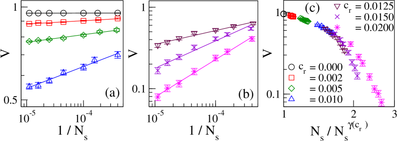
Figure 1: ${\rm V}$ versus $1/N_{s}$ plots in the (a) ordered and (b) disordered state for $\eta=0.10$. The error bars indicate standard error in mean. The solid lines show the respective algebraic fits. (c) Plot of ${\rm V}$ versus scaled system size $N_{s}/N_{s}^{\gamma}$ on log-log scale, where $\gamma$ is a function of $c_{r}$. The data shows good scaling for $0<c_{r}\leq 0.0125$, but deviates for $c_{r}\geq 0.0125$.

We numerically simulate the collection of $N_{s}$ SPPs spread over the $L\times L$ ($L\in[50,300]$) 2D substrate with periodic boundary condition. Initially the particles are chosen to have random velocity, but with constant speed ${v}_{s}$. The density of the SPPs and the RQRs are defined as $c_{s}=N_{s}/L^{2}$ and $c_{r}=N_{r}/L^{2}$, respectively. We distribute these rotators uniformly on the substrate, and randomly assign intrinsic orientation $\varphi\in[-\pi,\pi]$. In this system, the position and the velocity of all the SPPs are updated simultaneously following Eqs. (1) and (2). At every time step, we use OpenMP Application Program Interface for a parallel updating procedure of all the SPPs.

In this Rapid Communication, we consider $c_{s}=1.0$, $v_{s}=1.0$, and $\mu=1.0$. Moreover, we take $R_{s}=R_{r}=1$ for simplicity. In the absence of the rotators vicsek1995 , the system shows disorder to order transition with decreasing noise strength $\eta$. The ordering in the system is measured in terms of the conventional absolute value of the average normalized velocity

$${\rm V}=\langle\frac{1}{N_{s}{v}_{s}}|\sum_{i=1}^{N_{s}}{\bm{v}}_{i}|\rangle$$ (3)

of the entire system vicsek1995 . Here $\langle\cdot\rangle$ indicates an average over many realizations and time in the steady state. ${\rm V}$ varies from zero to unity for disorder to order state transition. For the reported data, we start the averaging of observables after $3\times 10^{5}$ updates to assure reaching the steady state, and averaging is done for the next $5\times 10^{5}$ updates. Up to $30$ realizations are used for better averaging.

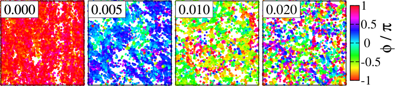
Figure 2: Steady-state snapshots are shown for $\eta=0.10$, $L=150$ and different $c_{r}$ as indicated on the respective panels. The color bar indicates orientation of the SPPs. The rotators with random intrinsic orientation are not shown for the clarity of the figure.

For a fixed $\eta$, we calculate ${\rm V}$ for different $c_{r}$, and study its variation with system size. As shown for $\eta=0.1$ in Fig. 1(a), in the clean system, ${\rm V}$ does not change with system size; consequently, the system possesses a nonzero ${\rm V}$ in the thermodynamic limit. Therefore, the clean system remains in the LRO state, which is a well-known phenomenon tonertu1998 . However, in the presence of the RQRs, ${\rm V}$ decreases algebraically with $N_{s}$ following the relation

$${\rm V}={\cal A}(c_{r})N_{s}^{-\nu(c_{r})},$$ (4)

as shown in Figs. 1(a) and 1(b). Here both ${\cal A}$ and $\nu$ are functions of $c_{r}$ for a fixed $\eta$. Therefore, in the thermodynamic limit, ${\rm V}$ of the system with RQRs reduces to zero. We stress that for small $c_{r}$ the system remains in a QLRO state, beyond which the AMQR shows a continuous QLRO-disorder state transition, as we will see shortly. In Fig. 2, we show snapshots of the orientation and the local density of the SPPs for $\eta=0.1$ and different $c_{r}$. For $c_{r}=0$, all the particles are in highly ordered state. RQRs perturb the LRO flocking as shown for $c_{r}=0.005,0.01$. For high density $c_{r}=0.02$, the SPPs remain highly disordered.

We further study the fluctuation in the orientation of the SPPs. The width of a normalized distribution $P(\phi)$ of orientation of the SPPs provides a measure of this fluctuation. It is calculated by averaging over the distributions at every time step in the steady state, and also over many realizations. While averaging, we set the mean orientation of all the distributions at $\phi=0$.

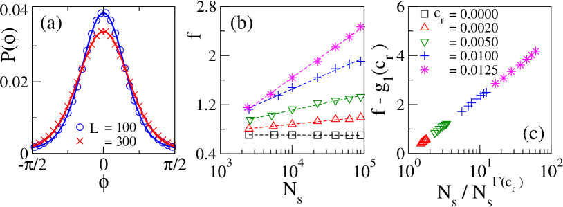
Figure 3: (a) Distribution $P(\phi)$ of the orientation of the SPPs is shown for $\eta=0.10$ and $c_{r}=0.005$. The curves are zoomed into the range $\phi\in[-\pi/2,\pi/2]$ for better visibility. The solid lines show the respective fits with Voigt profile. (b) Plot of the FWHM $f$ of $P({\phi})$ versus $N_{s}$. In the presence of quenched rotators, $f$ increases logarithmically with $N_{s}$. The dashed lines show respective fits. (c) Plot of shifted FWHM $f-g_{1}(c_{r})$ with scaled system size $N_{s}/N_{s}^{\Gamma}$, where both $g_{1}$ and $\Gamma$ are functions of $c_{r}$. The scaling holds good for $c_{r}\leq 0.0125$.

We note that $P(\phi)$ widens with the increasing density of RQRs. This is quite intuitive since the degree of disorder increases with $c_{r}$. We fit these distributions with a Voigt profile, which is defined as the convolution of the Gaussian and the Lorentzian functions voigt . A brief discussion of the Voigt profile and the procedure used to fit $P(\phi)$ with it are provided in Appendix A. From the respective fits, we calculate the full width at half maximum (FWHM) $f$ of the distributions.

We note that, in the clean system, $P(\phi)$ does not change with system size. However, for any fixed $c_{r}>0$, $P(\phi)$ widens with increasing system size, as shown in Fig. 3(a) for $(\eta,c_{r})=(0.10,0.005)$ (also see Appendix A). In Fig. 3(b), we show the variation of $f$ with system size for different $c_{r}$. For $c_{r}=0$, $f$ does not change with $N_{s}$. Therefore, in the clean system, the fluctuation in the orientation of the SPPs does not depend on the system size, and the system is in the LRO state. However, for $c_{r}>0$, FWHM of $P(\phi)$ follows the relation $f=g_{1}(c_{r})+g_{2}(c_{r})\ln(N_{s})$, where both $g_{1}$ and $g_{2}$ are functions of $c_{r}$. Since $g_{2}\geq 0$, $f$ increases logarithmically with $N_{s}$, which further confirms the QLRO in the AMQR.

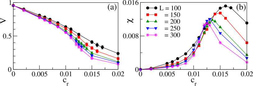
Figure 4: (a) Variation of ${\rm V}$ with $c_{r}$ shown for different system sizes and $\eta=0.10$. (b) Variance $\chi$ of ${\rm V}$ plotted with $c_{r}$. The peaks in the curves indicate the critical density of the rotators $c_{rc}(L)$ for the QLRO-disorder transition for the respective system sizes.

In Fig. 1(c), we plot ${\rm V}$ versus scaled system size $N_{s}/N_{s}^{\gamma(c_{r})}$ for $\eta=0.1$ and different $c_{r}$. Here $\gamma(c_{r})\simeq 1-kc_{r}$, where $k$ is a positive constant. Moreover, $\nu=z(1-\gamma)$, where $z$ is a nonmonotonic function of $\eta$. We note nice scaling collapse for $c_{r}\leq 0.0125$. This predicts that, for $c_{r}\leq 0.0125$, the system can be divided into sub-systems of size $N_{s}^{\gamma(c_{r})}$ within which the SPPs remain ordered. Since $\gamma=1$ for $c_{r}=0$, ${\rm V}$ does not depend on system size, and therefore the clean system remains in the LRO state. However, in the presence of RQRs, the system remains in the QLRO state. Moreover, the scaling predicts self-similarity of the system for different $c_{r}\leq 0.0125$. As shown in Fig. 3(c), we also find nice scaling collapse of $f-g_{1}(c_{r})$ with scaled system size $N_{s}/N_{s}^{\Gamma(c_{r})}$ for different $c_{r}\leq 0.0125$, where $\Gamma=1-g_{2}$ that varies linearly with $c_{r}$, for small $c_{r}$. Similar scaling holds for other $\eta$ values in the QLRO state.

In Fig. 4(a), we show the variation of ${\rm V}$ with $c_{r}$ for $\eta=0.1$ and different system sizes. Starting from the value of ${\rm V}$ close to $1$ for small $c_{r}$, ${\rm V}$ shows a transition to smaller values with increasing $c_{r}$. Therefore, with increasing $c_{r}$, QLRO-disorder transition occurs in the system. We further calculate the variance $\chi$ of ${\rm V}$ for different system sizes, and plot these as a function of $c_{r}$ in Fig. 4(b). Data shows systematic variation in $\chi$ as a function of $c_{r}$, and a peak appears at $c_{r}=c_{rc}(L)$ where the fluctuation in ${\rm V}$ is large. This suggests a continuous QLRO-disorder state transition in the AMQR. We consider $c_{rc}(L)$ as the critical density for the QLRO-disorder state transition for system size $L$. The position of the peak shifts from $c_{r}=0.016$ to $0.0125$ as $L$ is increased from $100$ to $300$. However, we note that $c_{rc}(L)$ flattens on increasing $L$ for all $\eta$ values. Using the extrapolated values $c_{rc}(L\rightarrow\infty)$, we construct a phase diagram in the $\eta$–$c_{r}$ plane. We stress that in the presence of RQRs, the system remains in the QLRO below the phase boundary shown in Fig. 5.

Figure 5: Phase diagram in noise strength versus density of rotator plane. For small $c_{r}$, the QLRO state prevails, beyond which the system continuously goes to the disorder state.

Long-distance and long-time properties of the SPPs with quenched obstacles can also be characterized using a hydrodynamic description of the model. The relevant hydrodynamic variables for this model are (i) SPP density $\rho({{\bm{r}},t})$ which is a globally conserved quantity and (ii) velocity ${\bm{v}}({{\bm{r}},t})$ which is a broken-symmetry parameter in the ordered state. These variables can be obtained by suitable coarsening of corresponding discrete variables in the microscopic model tonertu1995 ; tonertu1998 ; aparna2008 ; bertin2006 ; bertin2009 ; ihle2011 . Following the phenomenology of the system, we write the hydrodynamic equations of motion for the density and the velocity fields as

$$\partial_{t}\rho + \nabla\cdot({\bm{v}}\rho)=D_{\rho}\nabla^{2}\rho,$$ (5)

$$\partial_{t}{\bm{v}} + \lambda_{1}({\bm{v}}\cdot\nabla){\bm{v}}+\lambda_{2}(\nabla\cdot{\bm{v}}){\bm{v}}+\lambda_{3}\nabla({v}^{2})$$ (6)

$$= (\alpha_{1}-\alpha_{2}{v}^{2}){\bm{v}}-\nabla P+D_{B}\nabla(\nabla\cdot{\bm{v}})$$

$$\quad+D_{T}\nabla^{2}{\bm{v}}+D_{2}({\bm{v}}\cdot\nabla)^{2}{\bm{v}}+\frac{\rho_{o}}{\rho}{\bm{\zeta}}+{\bm{f}}.$$

${\bm{f}}$ represents the annealed noise term that provides a random driving force. We assume this to be a white Gaussian noise with the correlation

$$\langle f_{i}({\bm{r}},t)f_{j}({\bm{r}}^{\prime},t^{\prime})\rangle=\Delta\delta_{ij}\delta({\bm{r}}-{\bm{r}}^{\prime})\delta(t-t^{\prime}),$$ (7)

where $\Delta$ is a constant, and dummy indices $i,j$ denote Cartesian components. The effect of obstacles is contained in the term $\frac{\rho_{o}}{\rho}{\bm{\zeta}}$ in Eq. (6), where $\rho_{o}$ represents obstacle density, and ${\bm{\zeta}}({\bm{r}},t)$ signifies the obstacle field. We assume the correlation

$$\langle\zeta_{i}({\bm{r}},t)\zeta_{j}({\bm{r}}^{\prime},t^{\prime})\rangle=\zeta^{2}\delta_{ij}\delta({\bm{r}}-{\bm{r}}^{\prime}),$$ (8)

which contains no time dependence, and therefore represents a quenched noise. Equations (5)-(8) represent the Toner-Tu tonertu1998 model for $\zeta=0$.

We check whether a broken-symmetry state of the SPPs in the presence of the obstacle field survives to small fluctuation in the hydrodynamic fields. In the hydrodynamic limit, a linearized study of Eqs. (5) and (6) gives spatially Fourier transformed equal-time correlation functions for the density

$$C_{\rho\rho}({\bm{q}},t)=\frac{1}{q^{2}}\left\{\frac{\zeta^{2}\rho_{o}^{2}a_{\rho}(\theta)}{b(\theta)q^{2}+d(\theta)}+\Delta A_{\rho}(\theta)\right\}$$ (9)

and the velocity

$$C_{{vv}}({\bm{q}},t)=\frac{1}{q^{2}}\left\{\frac{\zeta^{2}\rho_{o}^{2}a_{v}(\theta)}{b(\theta)q^{2}+d(\theta)}+\Delta A_{v}(\theta)\right\}.$$ (10)

The parameters $a_{\rho,{v}}$, $A_{\rho,{v}}$, $b$, and $d$ depend on the specific microscopic model and the angle $\theta$ between the wave number ${\bm{q}}$ and the flocking direction. A detailed calculation for Eqs. (9) and (10) is given in Appendix B.Our result matches with the earlier prediction by Toner and Tu tonertu1998 for $\zeta=0$, where the two structure factors diverge as $1/q^{2}$ for small $q$. However, the linearized theory suggests $C_{\rho\rho,vv}\sim 1/q^{4}$ for $\zeta\neq 0$, provided $d(\theta)=0$. In general for a Vicsek-like model as our AMQR, $d(\theta)$ vanishes for certain directions $\theta=\theta_{c}$ or $\pi-\theta_{c}$, where $\theta_{c}$ depends on the model parameters. We stress that although the quenched inhomogeneities increase fluctuation in the system as compared to the clean case, the neglected nonlinearities suppress these higher order fluctuations so that a QLRO state can prevail. Alhough an exact nonlinear calculation is not practically feasible for the 2D polar flock toner2018 , presumption of convective nonlinearities as relevant terms offers a way out revtoner2005 ; tonertu1998 . A nonlinear calculation toner2018 following this presumption renormalizes diffusivities as $1/q$ so that the term $b(\theta)q^{2}$ in Eqs. (9) and (10) approaches a finite value, and therefore, a QLRO state exists in the system. This explanation is consistent with the giant number fluctuation revramaswamy2010 in the AMQR. We have checked that inclusion of the RQRs increases the fluctuation in the system as compared to the clean case. This enhanced fluctuation destroys the usual LRO of the clean system. However, we note that the fluctuation decreases with further increase in $c_{r}$ which disagrees with Eq. (9), as the linearized hydrodynamics prescribes an increase in the effect of quenched inhomogeneity with $\rho_{o}$. Therefore, the neglected nonlinearity indeed plays a pivotal role in stabilizing the QLRO state in the system. A detailed discussion of these phenomenologies is given in Appendix C.

In summary, we have studied the effect of random quenched rotators on the flocking state of polar SPPs. These rotators are one kind of obstacle that rotate the orientation of the SPPs. We find that, for small density of the rotators, the usual LRO of the clean polar SPPs is destroyed, and a QLRO state prevails. With further increase in density of the rotators, a continuous QLRO to disorder state transition takes place in the system. Our linearized hydrodynamic analysis predicts an anisotropic higher order fluctuation which destroys the usual LRO of the clean SPPs. However, the neglected nonlinearities suppress these fluctuations yielding a QLRO in the system. In equilibrium systems with random quenched obstacles, an ordered state does not exist below four dimensions imry1975 ; grinstein1976 . However, as compared to the equilibrium systems, in our model for polar SPPs with quenched rotators, we find QLRO in two-dimensions. Our prediction of the QLRO in the polar SPPs in the presence of quenched obstacles agrees with recent observations toner2018 ; chepizhko2013 .

In contrast to the LRO and the QLRO reported in Ref. chepizhko2013 , we note QLRO only, because of the basic difference in the nature of obstacles. The SPP-obstacle interaction in Ref. chepizhko2013 depends on the angle between their relative position vector and the orientation of the SPP. Therefore, this force is a continuous function of the orientation distribution of the SPPs. On the contrary, the quenched force offered by the obstacles in our model is random and discrete. However, similar to their results, we note the existence of an optimal noise for which the system attains the maximum ordering in the presence of quenched rotators (see Appendix D). Our model can be applied in natural systems like a shoal of fishes moving in the sea in the presence of vortices. An experiment on a collection of fishes living in a shallow water pool jolles2017 ; couzin2008 ; krause2018 ; puckett2018 , in the presence of uncorrelated artificial vortices, may verify our predictions.

S.M. acknowledges Sriram Ramaswamy for pointing out an important correction in the hydrodynamic calculation and Sanjay Puri for useful discussions. The authors thank John Toner for his useful comments and suggestions. S.M. also thanks S. N. Bose National Centre for Basic Sciences, Kolkata for providing kind hospitality, and the Department of Science and Technology, India for financial support. M.K. acknowledges financial support from the Department of Science and Technology, India under the Ramanujan Fellowship.

Appendix A Voigt profile and orientation fluctuation of Self-propelled particles

Voigt profile is defined as

$${\cal V}(\phi;\sigma,\epsilon)=\int_{-\pi}^{\pi}\frac{\exp(-\Phi^{2}/2\sigma^{2})}{\sigma\sqrt{2\pi}}\frac{\epsilon}{\pi\left[(\phi-\Phi)^{2}+\epsilon^{2}\right]}d\Phi,$$ (11)

where the Gaussian and the Lorentzian contributions are signified by the parameters $\sigma$ and $\epsilon$, respectively. The full width at half maximum (FWHM) of the Voigt profile is approximately given by the relation voigt

$$f\approx 0.5346f_{L}+\sqrt{0.2166f_{L}^{2}+f_{G}^{2}},$$ (12)

where $f_{L}=2\epsilon$ represents the FWHM of the Lorentzian distribution, and $f_{G}=2\sigma\sqrt{2\ln 2}$ represents the FWHM of the Gaussian distribution.

As mentioned in the main text, we realise that the distribution $P(\phi)$ follows Voigt profile. So we take discrete Fourier transform (DFT) of $P(\phi)$ and fit the transformed distribution with the characteristic function ${\xi}\left(n;\sigma,\epsilon\right)=\exp\left(\frac{\sigma^{2}n^{2}}{2}-\epsilon|n|\right)$ of ${\cal V}(\phi;\sigma,\epsilon)$. Here $n$ represents the Fourier conjugate of $\phi$. From the fits in the Fourier space, we extract the values of the parameters $\sigma$ and $\epsilon$, and calculate the FWHM of $P(\phi)$ using Eq. (12). The fits shown in Fig. 3(a) of the main text are obtained by the inverse DFT of the fitted functions ${\xi}\left(n;\sigma,\epsilon\right)$.

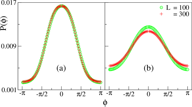
Figure 6: Plot of orientation distribution $P(\phi)$ of the SPPs for $\eta=0.40$. In the clean system, i.e., for $c_{r}=0$, the system remains in the banded state. As shown in (a), $P(\phi)$ does not change with system size in this state. However, as shown in (b) for $c_{r}=0.008$, fluctuation in ${\rm V}$ increases with system size. Respective fits with the Voigt profile has not been shown for the clarity of the plots.

We must stress here that, in the clean system, $P(\phi)$ is always independent of system size; no matter the system is in the homogeneous ordered state or in the banded state. This is evident from Fig. 6(a) where we plot $P(\phi)$ for the banded state ($\eta=0.40$). However, in the presence of random quenched rotators, $P(\phi)$ widens with system size, as shown in Fig. 6(b).

Appendix B Linearised theory of the broken symmetry state in the presence of quenched inhomogeneities

Given the equations of motion (EOMs) of the hydrodynamic fields in the main text, we check whether a broken symmetry state of the SPPs in the presence of obstacle field survives to small fluctuations in the hydrodynamic fields. We consider a broken symmetry state ${\bm{v}}={v}_{0}\hat{y}+\delta{\bm{v}}$, where the spontaneous average value of the velocity $\langle{\bm{v}}\rangle={v}_{0}\hat{y}$ and ${v}_{0}=\sqrt{\alpha_{1}/\alpha_{2}}$. Fluctuation in the density field is given by $\delta\rho=\rho-\bar{\rho}$, where $\bar{\rho}$ represents the mean density of SPPs. We expand spatial and temporal gradients appearing in the EOMs, and retain upto lowest-order terms in derivatives, since we are interested in long-time and long-distance behavior of the system. Doing so, we obtain the EOM for the fluctuation $\delta{v}_{y}$ as

$$\partial_{t}\delta{v}_{y}+2\alpha_{1}\delta{v}_{y}=-\sigma_{1}\partial_{y}\delta\rho+\frac{\rho_{o}}{\bar{\rho}}\zeta_{y}+\mbox{irrelevant terms}.$$ (13)

Since we are interested in hydrodynamic modes, i.e., modes for which frequency $\omega\rightarrow 0$ as wave number $q\rightarrow 0$, we can neglect time-variation of $\delta{v}_{y}$ as compared to its value. Therefore, from Eq. (13), we obtain the relation

$$\delta{v}_{y}=\frac{1}{2\alpha_{1}}\left(-\sigma_{1}\partial_{y}\delta\rho+\frac{\rho_{o}}{\bar{\rho}}\zeta_{y}\right).$$ (14)

Using the expression for $\delta{v}_{y}$ from Eq. (14), we obtain the EOMs for $\delta\rho$ and $\delta{v}_{x}$ as

$$\left(\partial_{t}+{v}_{0}\partial_{y}-D_{\rho y}\partial_{y}^{2}-D_{\rho}\partial_{x}^{2}\right)\delta\rho+\bar{\rho}\partial_{x}\delta{v}_{x} = -\frac{\rho_{o}}{2\alpha_{1}}\partial_{y}\zeta_{y},$$

$$\sigma_{1}\partial_{x}\delta\rho+\left(\partial_{t}+\gamma\partial_{y}-D_{L}\partial_{x}^{2}-D_{y}\partial_{y}^{2}\right)\delta{v}_{x} = \frac{\rho_{o}}{\bar{\rho}}\zeta_{x}+f_{x},$$

where $D_{\rho y}=D_{\rho}+\bar{\rho}\sigma_{1}/2\alpha_{1}$, $D_{L}=D_{B}+D_{T}$, $D_{y}=D_{T}+D_{2}{v}_{0}^{2}$ and $\gamma=\lambda_{1}{v}_{0}$. These parameters depend on the scalar quantities ${v}^{2}$ and $\rho({\bm{r}})$ whose fluctuations are small in the broken symmetry state. So, hereafter we consider these parameters as constants.

It is now instructive to Fourier transform the set of Eqs. (LABEL:eqmdelrho)-(LABEL:eqmdelvx) in space and time. Given a function $u({\bm{r}},t)$, its Fourier transform in space and time is defined as

$$u({\bm{q}},\omega)=\int_{-\infty}^{\infty}dtd{\bm{r}}e^{i\omega t}e^{-i{\bm{q}}\cdot{\bm{r}}}u({\bm{r}},t).$$ (17)

Using the above definition, we write the equations of motion for the fluctuations in the Fourier space as follow

$$\left[i\left(\omega-{v}_{0}q_{y}\right)-\Gamma_{\rho}({\bm{q}})\right]\delta\rho-i\bar{\rho}q_{x}\delta{v}_{x} = -i\frac{\rho_{o}}{2\alpha_{1}}q_{y}\zeta_{y},$$

$$i\sigma_{1}q_{x}\delta\rho+\left[-i\left(\omega-\gamma q_{y}\right)+\Gamma_{L}({\bm{q}})\right]\delta{v}_{x} = \frac{\rho_{o}}{\bar{\rho}}\zeta_{x}+f_{x},$$

where wave number dependent dampings are

$$\Gamma_{\rho}({\bm{q}}) = D_{\rho}q_{x}^{2}+D_{\rho y}q_{y}^{2},$$ (20)

$$\Gamma_{L}({\bm{q}}) = D_{L}q_{x}^{2}+D_{y}q_{y}^{2}.$$ (21)

The normal modes of the pair of coupled Eqs. (LABEL:eqfour1)-(LABEL:eqfour2) are two propagating sound waves with complex eigenfrequencies

$$\omega_{\pm}=c_{\pm}(\theta)q-i\Gamma_{L}\left[\frac{{v}_{\pm}(\theta)}{2c_{2}(\theta)}\right]-i\Gamma_{\rho}\left[\frac{{v}_{\mp}(\theta)}{2c_{2}(\theta)}\right],$$ (22)

where $\theta$ is the angle between ${\bm{q}}$ and the direction of flock, i.e., $\hat{y}$-direction, and

$$c_{\pm}(\theta) = \frac{\gamma+{v}_{0}}{2}\cos\theta\pm c_{2}(\theta),$$ (23)

$${v}_{\pm}(\theta) = c_{2}(\theta)\pm\frac{\gamma-{v}_{0}}{2}\cos\theta,$$ (24)

$$c_{2}(\theta) = \sqrt{\frac{1}{4}(\gamma-{v}_{0})^{2}\cos^{2}\theta+\sigma_{1}\bar{\rho}\sin^{2}\theta}.$$ (25)

Solving the linear set of Eqs. (LABEL:eqfour1)-(LABEL:eqfour2) for $\delta\rho({\bm{q}},\omega)$ and $\delta{v}_{x}({\bm{q}},\omega)$, we obtain

$$\left[\begin{array}[]{cc}\delta\rho({\bm{q}},\omega)\\ \delta{v}_{x}({\bm{q}},\omega)\end{array}\right]=\left[\begin{array}[]{cc}G_{\rho\rho}({\bm{q}},\omega)&G_{\rho L}({\bm{q}},\omega)\\ G_{L\rho}({\bm{q}},\omega)&G_{LL}({\bm{q}},\omega)\end{array}\right]\left[\begin{array}[]{cc}i\rho_{o}\zeta_{y}q_{y}/2\alpha\\ f_{x}+\rho_{o}\zeta_{x}/\bar{\rho}\end{array}\right]$$ (32)

(33)

where the propagators are

$$G_{\rho\rho}({\bm{q}},\omega) = \frac{-i\left(\omega-\gamma q\cos\theta\right)+\Gamma_{L}({\bm{q}})}{\left[\omega-c_{+}(\theta)q\right]\left[\omega-c_{-}(\theta)q\right]+i\omega\left[\Gamma_{\rho}({\bm{q}})+\Gamma_{L}({\bm{q}})\right]-iq\cos\theta\left[\gamma\Gamma_{\rho}({\bm{q}})+{v}_{0}\Gamma_{L}({\bm{q}})\right]},$$ (34)

$$G_{\rho L}({\bm{q}},\omega) = \frac{i\bar{\rho}q\sin\theta}{\left[\omega-c_{+}(\theta)q\right]\left[\omega-c_{-}(\theta)q\right]+i\omega\left[\Gamma_{\rho}({\bm{q}})+\Gamma_{L}({\bm{q}})\right]-iq\cos\theta\left[\gamma\Gamma_{\rho}({\bm{q}})+{v}_{0}\Gamma_{L}({\bm{q}})\right]},$$ (35)

$$G_{L\rho}({\bm{q}},\omega) = \frac{-i\sigma_{1}q\sin\theta}{\left[\omega-c_{+}(\theta)q\right]\left[\omega-c_{-}(\theta)q\right]+i\omega\left[\Gamma_{\rho}({\bm{q}})+\Gamma_{L}({\bm{q}})\right]-iq\cos\theta\left[\gamma\Gamma_{\rho}({\bm{q}})+{v}_{0}\Gamma_{L}({\bm{q}})\right]},$$ (36)

$$G_{LL}({\bm{q}},\omega) = \frac{i\left(\omega-{v}_{0}q\cos\theta\right)-\Gamma_{\rho}({\bm{q}})}{\left[\omega-c_{+}(\theta)q\right]\left[\omega-c_{-}(\theta)q\right]+i\omega\left[\Gamma_{\rho}({\bm{q}})+\Gamma_{L}({\bm{q}})\right]-iq\cos\theta\left[\gamma\Gamma_{\rho}({\bm{q}})+{v}_{0}\Gamma_{L}({\bm{q}})\right]}.$$ (37)

Using the expression given in Eqs. (33)-(37) and the correlations given in the main text, we calculate correlation functions for the density and the velocity fields. Retaining upto lowest-order terms in $q$, we obtain density-density correlation function

$$C_{\rho\rho}({\bm{q}},\omega) = \frac{\left(\omega-\gamma q\cos\theta\right)^{2}\left[-\frac{\rho_{o}^{2}}{4\alpha_{1}^{2}}\zeta^{2}q^{2}\cos^{2}\theta\delta(\omega)\right]+\bar{\rho}^{2}q^{2}\sin^{2}\theta\left[\Delta+\frac{\rho_{o}^{2}}{\bar{\rho}^{2}}\zeta^{2}\delta(\omega)\right]}{\left[\omega-c_{+}(\theta)q\right]^{2}\left[\omega-c_{-}(\theta)q\right]^{2}+\left\{\omega\left[\Gamma_{\rho}({\bm{q}})+\Gamma_{L}({\bm{q}})\right]-q_{y}\left[\gamma\Gamma_{\rho}({\bm{q}})+{v}_{0}\Gamma_{L}({\bm{q}})\right]\right\}^{2}},$$ (38)

and velocity-velocity correlation function

$$C_{{vv}}({\bm{q}},\omega) = \frac{-\sigma_{1}^{2}\zeta^{2}q^{4}\sin^{2}2\theta\frac{\rho_{o}^{2}}{16\alpha_{1}^{2}}\delta({\omega})+\left(\omega-{v}_{0}q\cos\theta\right)^{2}\left[\Delta+\frac{\rho_{o}^{2}}{\bar{\rho}^{2}}\zeta^{2}\delta(\omega)\right]}{\left[\omega-c_{+}(\theta)q\right]^{2}\left[\omega-c_{-}(\theta)q\right]^{2}+\left\{\omega\left[\Gamma_{\rho}({\bm{q}})+\Gamma_{L}({\bm{q}})\right]-q_{y}\left[\gamma\Gamma_{\rho}({\bm{q}})+{v}_{0}\Gamma_{L}({\bm{q}})\right]\right\}^{2}}.$$ (39)

Given these Fourier transformed correlation functions, we proceed further to obtain the spatially Fourier transformed equal-time correlation functions for the density and the velocity fields. Neglecting the higher order fluctuations, we obtain the expressions for $C_{\rho\rho,vv}({\bm{q}},t)$, as also given in the main text :

$$C_{\rho\rho}({\bm{q}},t)=\frac{1}{q^{2}}\left\{\frac{\zeta^{2}\rho_{o}^{2}a_{\rho}(\theta)}{b(\theta)q^{2}+d(\theta)}+\Delta A_{\rho}(\theta)\right\},$$ (40)

$$C_{{vv}}({\bm{q}},t)=\frac{1}{q^{2}}\left\{\frac{\zeta^{2}\rho_{o}^{2}a_{v}(\theta)}{b(\theta)q^{2}+d(\theta)}+\Delta A_{v}(\theta)\right\},$$ (41)

where

$$b(\theta) = \cos^{2}\theta\{\gamma\left(D_{\rho}\sin^{2}\theta+D_{\rho y}\cos^{2}\theta\right)$$ (42)

$$\qquad\qquad+{v}_{0}\left(D_{L}\sin^{2}\theta+D_{y}\cos^{2}\theta\right)\}^{2},$$

$$d(\theta) = \gamma{v}_{0}\cos^{2}\theta-\sigma_{1}\bar{\rho}\sin^{2}\theta,$$ (43)

$$p_{\pm}(\theta) = 2c_{2}\{c_{\pm}[(D_{L}+D_{\rho})\sin^{2}\theta+(D_{y}+D_{\rho y})\cos^{2}\theta]$$ (44)

$$\qquad-\cos\theta[({v}_{0}D_{L}+\gamma D_{\rho})\sin^{2}\theta$$

$$\qquad\qquad\qquad+({v}_{0}D_{y}+\gamma D_{\rho y})\cos^{2}\theta]\},$$

$$s_{\pm}(\theta) = (c_{\pm}-{v}_{0}\cos\theta)^{2}/2\pi,$$ (45)

$$s(\theta) = \bar{\rho}^{2}\sin^{2}\theta/2\pi,$$ (46)

$$a_{\rho}(\theta) = \sin^{2}\theta/2\pi,$$ (47)

$$A_{\rho}(\theta) = s(\theta)\left[\frac{1}{p_{+}(\theta)}+\frac{1}{p_{-}(\theta)}\right],$$ (48)

$$a_{v}(\theta) = {v}_{0}^{2}\cos^{2}\theta/2\pi\bar{\rho}^{2},$$ (49)

$$A_{v}(\theta) = \left[\frac{s_{+}(\theta)}{p_{+}(\theta)}+\frac{s_{-}(\theta)}{p_{-}(\theta)}\right].$$ (50)

Appendix C Effect of nonlinear terms

Linearised hydrodynamics suggests that $C_{\rho\rho,vv}\sim 1/q^{4}$ for small $q$ if $d(\theta)=0$, otherwise $C_{\rho\rho,vv}\sim 1/q^{2}$. It is clear from Eq. (43) that $d(\theta)$ cannot vanish for $u=\gamma v_{0}/\sigma_{1}\bar{\rho}<0$. Also for the case $u>0$, $d(\theta)$ vanishes only for $\theta=\theta_{c}$ and $\pi-\theta_{c}$, where $\theta_{c}=\tan^{-1}\sqrt{u}$. Therefore, the appearance of the $1/q^{4}$ divergence, as predicted by the linearized calculation, is relevant only for the case $u>0$, and that too along the two specific directions mentioned above.

Let us first discuss about the physical significance of the sign of $u$. The sign of $u=\gamma v_{0}/\sigma_{1}\bar{\rho}$ depends on the microscopic parameters of the concerned model. In general for Vicsek-like models, $u>0$ which infers that the pure modes for the velocity and the density fields are more or less in phase. However, there can be situation where these pure modes are almost in opposite phases inferring $u<0$, which we shall not discuss here. Since, our numerical model in this paper is a modification of the Vicsek model (VM), we stress that $u>0$ in our model. Then the immediate question arises if the higher order divergence predicted by the linearized calculation destabilises the QLRO that we claim for. Here we ascertain that the neglected nonlinear terms of the hydrodynamic EOMs make the existence of the QLRO possible in the system.

A common method to incorporate the effect of different nonlinearities is to first find out the dominating terms by ‘power counting’ tonertu1995 ; tonertu1998 ; toner2012 ; toner2018 . Unfortunately, that technique is not useful in our case, as it predicts all the nonlinearities as equally significant in 2D. Furthermore, a complete renormalisation group analysis is not practically feasible toner2018 ; However, if we assume that $\lambda_{1}$ term of the velocity EOM in the main text is the most relevant nonlinearity, then one can calculate the exact exponents for the model. Though this seems like an ad hoc assumption, a similar assumption practically works well in the presence of ${\bm{f}}$ (annealed) noise only. Therefore, one can proceed with this assumption for the quenched case also, as recently done by Toner et al. toner2018 but considering few more extra terms in the EOMs toner2012 . Though these extra terms are allowed by the symmetry of the system, but these terms do not change the system phenomenology further toner2012 . Therefore, the calculation done in Ref. toner2018 equally holds for our model also, which predicts that the $\lambda_{1}$ nonlinearity renormalizes the diffusivities as $1/q$ for small $q$. Therefore, from Eq. (42) we can see that $b(\theta)\sim 1/q^{2}$. Hence, the product $b(\theta)q^{2}$ approaches a finite value. Therefore, though the linearized calculation predicts highly anisotropic $C_{\rho\rho,vv}$, the convective nonlinearity suppresses that anisotropy, and makes the QLRO possible in our system.

The effect of nonlinearities in suppression of the higher order fluctuations predicted by the linearized theory can also be understood by the number fluctuation $\Delta N=\sqrt{\langle N^{2}\rangle-\langle N\rangle^{2}}$ in the AMQR. We note that in the clean system, $\Delta N\sim\langle N\rangle^{\kappa}$ with $\kappa>1/2$. In the presence of the RQRs also, the system shows giant number fluctuation, but $\kappa$ varies with $c_{r}$. We note that the number fluctuation for small $c_{r}$ is higher than the clean case. However, the fluctuation decreases with further increase in $c_{r}$, which is not allowed by Eq. (40) as the quenched terms should dominate over the annealed terms with increasing density of inhomogeneity. This observation suggests that the neglected nonlinearities play pivotal role in stabilizing ordered state in the system. Moreover, the scaling of the order parameter ${\rm V}$ with system size, as described in the main text, ensures us about the existence of the QLRO (and not the LRO) in the presence of quenched inhomogeneities.

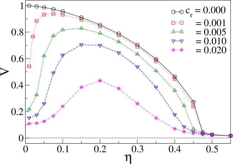
Figure 7: Plot of average normalized velocity versus noise strength shown for $L=100$ and different density of the rotators. While ${\rm V}$ decreases monotonically with increasing $\eta$ for the clean system, in the presence of the rotators, a certain amount of noise maximizes the ordering.

Appendix D Optimal noise

In Fig. 7, we show the variation of ${\rm V}$ with $\eta$ in the AMQR. In the clean system, ${\rm V}$ decays monotonically with increasing $\eta$. Surprisingly, in the presence of the RQRs, a certain amount of noise facilitates flocking, and below that the ordering reduces again. This happens because, in the presence of the RQRs, the system must have a non-zero noise to transfer the information of one sub-flock to another. Similar phenomenon has earlier been reported in Ref. chepizhko2013 .

References

- (1) T. Vicsek, A. Czirók, E. Ben-Jacob, I. Cohen, and O. Shochet, Phys. Rev. Lett. 75, 1226 (1995).
- (2) M. C. Marchetti, J. F. Joanny, S. Ramaswamy, T. B. Liverpool, J. Prost, Madan Rao, and R. Aditi Simha, Rev. Mod. Phys. 85, 1143 (2013).
- (3) J. Toner, Y. Tu, and S. Ramaswamy, Ann. Phys. 318, 170 (2005).
- (4) S. Ramaswamy, Annu. Rev. Cond. Matt. Phys. 1, 323 (2010).
- (5) T. Vicsek and A. Zafeiris, Phys. Rep. 517, 71 (2012).
- (6) M. E. Cates, Rep. Prog. Phys. 75, 042601 (2012).
- (7) J. Toner and Y. Tu, Phys. Rev. Lett. 75, 4326 (1995).
- (8) J. Toner and Y. Tu, Phys. Rev. E 58, 4828 (1998).
- (9) S. Mishra, A. Baskaran and C. Marchetti, Phys. Rev. E 81, 061916 (2010).
- (10) H. Chaté, F. Ginelli, G. Grégoire and F. Raynaud, Phys. Rev. E 77, 046113 (2008).
- (11) A. Morin, N. Desreumaux, J. B. Caussin, and D. Bartolo, Nat. Phys. 13, 63 (2017).
- (12) O. Chepizhko, E. G. Altmann and F. Peruani, Phys. Rev. Lett. 110, 238101 (2013).
- (13) D. Yllanes, M. Leoni and M. C. Marchetti, New J. Phys. 19, 103026 (2017).
- (14) D. A. Quint and A. Gopinathan, Phys. Biol. 12, 046008 (2015).
- (15) Cs. Sándor, A. Libál, C. Reichhardt and C. J. O. Reichhardt, Phys. Rev. E 95, 032606 (2017).
- (16) C. J. O. Reichhardt and C. Reichhardt, Nat. Phys. 13, 10 (2017).
- (17) Y. Imry and S. K. Ma, Phys. Rev. Lett. 35, 1399 (1975).
- (18) G. Grinstein and A. Luther, Phys. Rev. B 13, 1329 (1976).
- (19) P. M. Chaikin and T. C. Lubensky, Principles of Condensed Matter Physics (Cambridge University Press, Cambridge, 1998).
- (20) J. J. Olivero and R. L. Longbothum, J. Quant. Spectrosc. Radiat. Transfer 17, 233 (1977).
- (21) A. Baskaran, J. W. Dufty and J. J. Brey, Phys. Rev. E 77, 031311 (2008).
- (22) E. Bertin, M. Droz and G. Grégoire, Phys. Rev. E 74, 022101 (2006).
- (23) E. Bertin, M. Droz and G. Grégoire, J. Phys. A: Math. Theor. 42, 445001 (2009).
- (24) T. Ihle, Phys. Rev. E 83, 030901(R) (2011).
- (25) J. Toner, N. Guttenberg and Y. Tu, arXiv:1805.10324v1 [cond-mat.stat-mech]; arXiv:1805.10326v1 [cond-mat.stat-mech].
- (26) D. J. T. Sumpter, J. Krause, R. James, I. D. Couzin and A. J. W. Ward, Curr. Biol. 18, 1773 (2008).
- (27) J. W. Jolles, N. J. Boogert, V. H. Sridhar, I. D. Couzin and A. Manica, Curr. Biol. 27, 2862 (2017).
- (28) L. Snijders, R. H. J. M. Kurvers, I. W. Ramnarine and J. Krause, Nat. Ecol. Evol. 2, 1610 (2018).
- (29) J. G. Puckett, A. R. Pokhrel and J. A. Giannini, Sci. Rep. 27, 7587 (2018).
- (30) J. Toner, Phys. Rev. E 86, 031918 (2012).