Bandwidth Partitioning and Downlink Analysis in Millimeter Wave Integrated Access and Backhaul for 5G

Abstract

With the increasing network densification, it has become exceedingly difficult to provide traditional fiber backhaul access to each cell site, which is especially true for small cell base stations (SBSs). The increasing maturity of millimeter wave (mm-wave) communication has opened up the possibility of providing high-speed wireless backhaul to such cell sites. Since mm-wave is also suitable for access links, the third generation partnership project (3GPP) is envisioning an integrated access and backhaul (IAB) architecture for the fifth generation (5G) cellular networks in which the same infrastructure and spectral resources will be used for both access and backhaul. In this paper, we develop an analytical framework for IAB-enabled cellular network using which its downlink rate coverage probability is accurately characterized. Using this framework, we study the performance of three backhaul bandwidth (BW) partition strategies: 1) equal partition: when all SBSs obtain equal share of the backhaul BW; 2) instantaneous load-based partition: when the backhaul BW share of an SBS is proportional to its instantaneous load; and 3) average load-based partition: when the backhaul BW share of an SBS is proportional to its average load. Our analysis shows that depending on the choice of the partition strategy, there exists an optimal split of access and backhaul BW for which the rate coverage is maximized. Further, there exists a critical volume of cell-load (total number of users) beyond which the gains provided by the IAB-enabled network disappear and its performance converges to that of the traditional macro-only network with no SBSs.

I Introduction

With the exponential rise in data-demand far exceeding the capacity of the traditional macro-only cellular network operating in sub-6 GHz bands, network densification using mm-wave base stations (BSs) is becoming a major driving technology for the 5G wireless evolution [2]. While heterogeneous cellular networks (HetNets) with low power SBSs overlaid with traditional macro BSs improve the spectral efficiency of the access link (the link between a user and its serving BS), mm-wave communication can further boost the data rate by offering high bandwidth. That said, one of the main hindrances in the way of large-scale deployment of small cells is that the existing high-speed optical fiber backhaul network that connects the BSs to the network core is not scalabale to the extent of ultra-densification envisioned for small cells [3, 4, 5]. However, with recent advancement in mm-wave communication with highly directional beamforming [6, 7], it is possible to replace the so-called last-mile fibers for SBSs by establishing fixed mm-wave backhaul links between the SBS and the MBS equipped with fiber backhaul, also known as the anchored BS (ABS), thereby achieving Gigabits per second (Gbps) range data rate over backhaul links [8]. While mm-wave fixed wireless backhaul is targetted to be a part of the first phase of the commercial roll-out of 5G [9], 3GPP is exploring a more ambitious solution of IAB where the ABSs will use the same spectral resources and infrastructure of mm-wave transmission to serve cellular users in access as well as the SBSs in backhaul [10]. In this paper, we develop a tractable analytical framework for IAB-enabled mm-wave cellular networks using tools from stochastic geometry and obtain some design insights that will be useful for the ongoing pre-deployment studies on IAB.

I-A Background and related works

Over recent years, stochastic geometry has emerged as a powerful tool for modeling and analysis of cellular networks operating in sub-6 GHz [11]. The locations of the BSs and users are commonly modeled as independent Poisson point processes (PPPs) over an infinite plane. This model, initially developed for the analysis of traditional macro-only cellular networks [12], was further extended for the analysis of HetNets in [13, 14, 15, 16]. In the followup works, this PPP-based HetNet model was used to study many different aspects of cellular networks such as load balancing, BS cooperation, multiple-input multiple-output (MIMO), energy harvesting, and many more. Given the activity this area has seen over the past few areas, any attempt towards summarizing all key relevant prior works here would be futile. Instead, it would be far more beneficial for the interested readers to refer to dedicated surveys and tutorials [17, 18, 19, 20] that already exist on this topic. While these initial works were implicitly done for cellular networks operating in the sub-6 GHz spectrum, tools from stochastic geometry have also been leveraged further to characterize their performance in the mm-wave spectrum [21, 22, 23, 24]. These mm-wave cellular network models specifically focus on the mm-wave propagation characteristics which signifantly differ from those of the sub-6 GHz [6], such as the severity of blocking of mm-wave signals by physical obstacles like walls and trees, directional beamforming using antenna arrays, and inteference being dominated by noise [25]. These initial modeling approaches were later extended to study different problems specific to mm-wave cellular networks, such as, cell search [26], antenna beam alignment [27], and cell association in the mm-wave spectrum [28]. With this brief introduction, we now shift our attention to the main focus of this paper which is IAB in mm-wave cellular networks. In what follows, we provide the rationale behind mm-wave IAB and how stochastic geometry can be used for its performance evaluation.

For traditional cellular networks, it is reasonable to assume that the capacity achieved by the access links is not limited by the backhaul constraint on the serving BS since all BSs have access to the high capacity wired backhaul. As expected, backhaul constraint was ignored in almost all prior works on stochastic geometry-based modeling and analysis of cellular networks. However, with the increasing network densification with small cells, it may not be feasible to connect every SBS to the wired backhaul network which is limited by cost, infrastructure, maintenance, and scalability. These limitations motivated a significant body of research works on the expansion of the cellular networks by deploying relay nodes connected to the ABS by wireless backhaul links, e.g. see [29]. Among different techniques of wireless backhaul, 3GPP included layer 3 relaying as a part of the long term evolution advanced (LTE-A) standard in Release 10 [30, 31] for coverage extension of the cellular network. Layer 3 relaying follows the principle of IAB architecture, which is often synonymously referred to as self-backhauling, where the relay nodes have the functionality of SBS and the ABS multiplexes its time-frequency resources to establish access links with the users and wireless backhaul links with SBSs that may not have access to wired backhaul [32]. However, despite being the part of the standard, layer 3 relays have never really been deployed on a massive scale in 4G mostly due to the spectrum shortage in sub-6 GHz. For instance, in urban regions with high capacity demands, the operators are not willing to relinquish any part of the cellular bandwidth (costly and scarce resource) for wireless backhaul. However, with recent advancement in mm-wave communication, IAB has gained substantial interest since spectral bottleneck will not be a primary concern once high bandwidth in mm-wave spectrum (at least 10x the cellular BW in sub-6 GHz) is exploited. Some of the notable industry initiatives driving mm-wave IAB are mm-wave small cell access and backhauling (MiWaveS) [33] and 5G-Crosshaul [34]. In 2017, 3GPP also started working on a new study item to investigate the performance of IAB-enabled mm-wave cellular network [10].

Although backhaul is becoming a primary bottleneck of cellular networks, there is very little existing work on the stochastic geometry-based analyses considering the backhaul constraint [35, 36, 37]. While these works are focused on the traditional networks in sub-6 GHz, contributions on IAB-enabled mm-wave HetNet are even sparser, except an extension of the PPP-based model [38], where the authors modeled wired and wirelessly backhauled BSs and users as three independent PPPs. In [39, 40], similar modeling approach was used to study IAB in sub-6 GHz using full duplex BSs. The fundamental shortcoming of these PPP-based models is the assumption of independent locations of the BSs and users which are spatially coupled in actual networks. For instance, in reality, the users form spatial clusters, commonly known as user hotspots and the centers of the user hotspots are targetted as the potential cell-cites of the short-range mm-wave SBSs [41]. Not surprisingly, such spatial configurations of users and BSs are at the heart of the 3GPP simulation models [42]. To address this shortcoming of the analytical models, in this paper, we propose the first 3GPP-inspired stochastic geometry-based finite network model for the performance analysis of HetNets with IAB. The key contributions are summarized next.

I-B Contributions and outcomes

I-B1 New tractable model for IAB-enabled mm-wave HetNet

We develop a realistic and tractable analytical framework to study the performance of IAB-enabled mm-wave HetNets. Similar to the models used in 3GPP-compliant simulations [10], we consider a two-tier HetNet where a circular macrocell with ABS at the center is overlaid by numerous low-power small cells. The users are assumed to be non-uniformly distributed over the macrocell forming hotspots and the SBSs are located at the geographical centers of these user hotspots. The non-uniform distribution of the users and the spatial coupling of their locations with those of the SBSs means that the analysis of this setup is drastically different from the state-of-the-art PPP-based models. Further, the consideration of a single macrocell (justified by the noise-limited nature of mm-wave communications), allows us to glean crisp insights into the coverage zones, which further facilitate a novel analysis of load on ABS and SBSs. Assuming that the total system BW is partitioned into two splits for access and backhaul communication, we use this model to study the performance of three backhaul BW partition strategies, namely, (i) equal partition, where each SBS gets equal share of BW irrespective of its load, (ii) instantaneous load-based partition, where the ABS frequently collects information from the SBSs on their instantaneous loads and partitions the backhaul BW proportional to the instantaneous load on each SBS, and (iii) average load-based partition, where the ABS collects information from the SBSs on their average loads and partitions the backhaul BW proportional to the average load on each SBS.

I-B2 New load modeling and downlink rate analysis

For the purpose of performance evaluation and comparisons between the aforementioned strategies, we evaluate the downlink rate coverage probability i.e. probability that the downlink data rate experienced by a randomly selected user will exceed a target data rate. As key intermediate steps of our analysis we characterize the two essential components of rate coverage, which are (i) signal-to-noise-ratio ($\mathtt{SNR}$)-coverage probability, and (ii) the distribution of ABS and SBS load, which directly impacts the amount of resources allocated by the serving BS to the user of interest. We compute the probability mass functions (PMFs) of the ABS and the SBS loads assuming the number of users per hotspot is fixed. We then relax this fixed user assumption by considering independent Poisson distribution on the number of users in each hotspot. Due to a significantly different spatial model, our approach of load modeling is quite different from the load-modeling in PPP-based networks [37].

I-B3 System design insights

Using the proposed analytical framework, we obtain the following system design insights.

• We compare the three backhaul BW partition strategies in terms of three metrics, (i) rate coverage probability, (ii) median rate, and (iii) $5^{th}$ percentile rate. Our numerical results indicate that for a given combination of the backhaul BW partition strategy and the performance metric of interest, there exists an optimal access-backhaul BW split for which the metric is maximized.

• Our results demonstrate that the optimal access-backhaul partition fractions for median and $5^{th}$ percentile rates are not very sensitive to the choice of backhaul BW partition strategies. Further, the median and $5^{th}$ percentile rates are invariant to system BW.

• For given infrastructure and spectral resources, the IAB-enabled network outperforms the macro-only network with no SBSs up to a critical volume of total cell-load, beyond which the performance gains disappear and its performance converges to that of the macro-only network. Our numerical results also indicate that this critical total cell-load increases almost linearly with the system BW.

II System Model

II-A mm-wave Cellular System Model

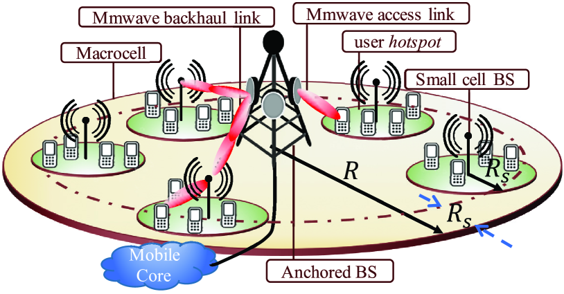
(a) User and BS locations

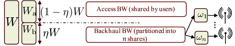
(b) Resource Allocation

Figure 1: Illustration of the system model.

II-A1 BS and user locations

Inspired by the spatial configurations used in 3GPP simulations [10, 42] for a typical outdoor deployment scenario of a two-tier HetNet, we assume that $n$ SBSs are deployed inside a circular macrocell of radius $R$ (denoted by $b({\bf 0},R)$) with the macro BS at its center. We assume that this BS is connected to the core network with high speed optical fiber and is hence an ABS. Note that, in contrast to the infinite network models (e.g. the PPP-based networks defined over $\mathbb{R}^{2}$) which are suitable for interference-dominated networks (such as conventional cellular networks in sub-6 GHz), we are limiting the complexity of the system model by considering single macrocell. This assumption is justified by the noise-limited nature of mm-wave communications [25]. Moreover, as will be evident in the sequel, this setup will allow us to glean crisp insights into the properties of this network despite a more general user distribution model (discussed next) compared to the PPP-based model.

We model a user hotspot at ${\bf x}$ as $b({\bf x},R_{\rm s})$, i.e., a circle of radius $R_{\rm s}$ centered at ${\bf x}$. We assume that the macrocell contains $n$ user hotspots, located at $\{{\bf x}_{i}\equiv(x_{i},\varphi_{i}),i=1,\dots,n\}$, which are distributed uniformly at random in $b({\bf 0},R-R_{\rm s})$. Thus, $\{{\bf x}_{i}\}$ is a sequence of independently and identically distributed (i.i.d.) random vectors with the distribution of ${\bf x}_{i}$ being:

$$f_{\bf X}({\bf x}_{i})=\begin{cases}\frac{x_{i}}{\pi(R-R_{\rm s})^{2}},&\text{when }0<x_{i}\leq R-R_{\rm s},0<\varphi_{i}\leq 2\pi,\\ 0,&\text{otherwise.}\end{cases}$$ (1)

The marginal probability density function (PDF) of $x_{i}$ is obtained as: $f_{X}(x_{i})=2x_{i}/(R-R_{\rm s})^{2}$ for $0<x_{i}\leq R-R_{\rm s}$ and $\varphi_{i}$ is a uniform random variable in $(0,2\pi]$. Note that this construction ensures that all hotspots lie entirely inside the macrocell, i.e., $b({\bf x}_{i},R_{\rm s})\cap b({\bf 0},R)^{c}=\varnothing,\ \forall\ i$. We assume that the number of users in the hotspot centered at ${\bf x}_{i}$ is $N_{{\bf x}_{i}}$, where case $1$: $N_{{\bf x}_{i}}=\bar{m}$ is fixed and equal for all $i=1,\dots,n$ and case $2$: $\{N_{{\bf x}_{i}}\}$ is a sequence of i.i.d. Poisson random variables with mean $\bar{m}$. These ${N}_{{\bf x}_{i}}$ users are assumed to be located uniformly at random independently of each other in each hotspot. Thus, the location of a user belonging to the hotspot at ${\bf x}_{i}$ is denoted by ${\bf x}_{i}+{\bf u}$, where ${\bf u}\equiv(u,\xi)$ is a random vector in $\mathbb{R}^{2}$ with PDF:

$$f_{\bf U}({\bf u})=\begin{cases}\frac{u}{\pi R_{\rm s}^{2}},&\text{when }0<{u}\leq R_{\rm s},0<\xi\leq 2\pi\\ 0,&\text{otherwise.}\end{cases}$$ (2)

The marginal PDF of $u$ is: $f_{U}(u)=2u/R_{\rm s}^{2}$ for $0<u\leq R_{\rm s}$ and $\xi$ is a uniform random variable in $(0,2\pi]$. We assume that the SBSs are deployed at the center of user hotspots, i.e., at $\{{\bf x}_{i}\}$. The ABS provides wireless backhaul to these SBSs over mm-wave links. See Fig. 1(a) for an illustration. Having defined the spatial distribution of SBSs and users, we now define the typical user for which we will compute the rate coverage probability. The typical user is a user chosen uniformly at random from the network. The hotspot to which the typical user belongs is termed as the representative hotspot. We denote the center of representative hotspot as ${\bf x}$, where ${\bf x}={\bf x}_{n}$, without loss of generality and the location of the typical user as ${\bf x}+{\bf u}$. For case $1$, the number of users in the representative cluster is $N_{\bf x}=N_{{\bf x}_{n}}=\bar{m}$. For case $2$, although $N_{{\bf x}_{i}}$ is i.i.d. Poisson, $N_{\bf x}$ does not follow the same distribution since the typical user will more likely belong to a hotspot with more number of users [43]. If $n\to\infty$, $N_{\bf x}$ follows a weighted Poisson distribution with PMF ${\mathbb{P}}(N_{\bf x}=k)=\frac{\bar{m}^{k-1}e^{-\bar{m}}}{(k-1)!}$, where, $k\in{\mathbb{Z}}^{+}$. It can be easily shown that if $N_{\bf x}$ follows a weighted Poisson distribution, we have $N_{\bf x}=N_{{\bf x}_{n}}+1$. Hence, for $n\to\infty$, one can obtain the distribution of $N_{\bf x}$ by first choosing a hotspot uniformly at random and then adding one user to it. However, when $n$ is finite, $N_{\bf x}$ will lie between $N_{{\bf x}_{n}}$ and $N_{{\bf x}_{n}}+1$ ($N_{{\bf x}_{n}}\leq N_{\bf x}\leq N_{{\bf x}_{n}}+1$). The lower bound on $N_{\bf x}$ is trivially achieved when $n=1$. Since the actual distribution of $N_{\bf x}$ for finite number of hotspots ($n>1$) is not tractable, we fix the typical user for case $2$ according to the following Remark.

Remark 1.

For case $2$, we first choose a hotspot centered at ${\bf x}$ uniformly at random from $n$ hotspots, call it the representative hotspot, and then add the typical user at ${\bf x}+{\bf u}$, where $\bf u$ follows the PDF in (2). Although this process of selecting the typical user is asymptotically exact when $N_{{\bf x}_{i}}\stackrel{{\scriptstyle i.i.d.}}{{\sim}}{\tt Poisson}(\bar{m}),\ \forall\ i=1,2,\dots,n$, and $n\to\infty$, it will have negligible impact on the analysis since our interest will be in the cases where the macrocells have moderate to high number of hotspots [44].

II-A2 Propagation assumptions

All backhaul and access transmissions are assumed to be performed in mm-wave spectrum. We assume that the ABS and SBS transmit at constant power spectral densities (PSDs) $P_{\rm m}/W$ and $P_{\rm s}/W$, respectively over a system BW $W$. The received power at ${\bf z}$ is given by $P\psi hL({\bf z},{\bf y})^{-1}$, where $P$ is a generic variable denoting transmit power with $P\in\{P_{\rm m},P_{\rm s}\}$, $\psi$ is the combined antenna gain of the transmitter and receiver, and $L({\bf z},{\bf y})=10^{((\beta+10\alpha\log_{10}\|{\bf z}-{\bf y}\|)/10)}$ is the associated pathloss. We assume that all links undergo i.i.d. Nakagami-$m$ fading. Thus, $h\sim{\tt Gamma}(m,m^{-1})$.

II-A3 Blockage model

Since mm-wave signals are sensitive to physical blockages such as buildings, trees and even human bodies, the LOS and NLOS path-loss characteristics have to be explicitly included into the analysis. On similar lines of [45], we assume exponential blocking model. Each mm-wave link of distance $r$ between the transmitter (ABS/SBS) and receiver (SBS/user) is LOS or NLOS according to an independent Bernoulli random variable with LOS probability $p(r)=\exp(-r/\mu)$, where $\mu$ is the LOS range constant that depends on the geometry and density of blockages. Since the blockage environment seen by the links between the ABS and SBS, SBS to user and ABS to user may be very different, one can assume three different blocking constants $\{\mu_{\rm b},\mu_{\rm s},\mu_{\rm m}\}$, respectively instead of a single blocking constant $\mu$. As will be evident in the technical exposition, this does not require any major changes in the analysis. However, in order to keep our notational simple, we will assume the same $\mu$ for all the links in this paper. Also, LOS and NLOS links may likely follow different fading statistics, which is incorporated by assuming different Nakagami-$m$ parameters for LOS and NLOS, denoted by $m_{L}$ and $m_{NL}$, respectively.

We assume that all BSs are equipped with steerable directional antennas and the user equipments have omni-directional antenna. Let $G$ be the directivity gain of the transmitting and receiving antennas of the BSs (ABS and SBS). Assuming perfect beam alignment, the effective gains on backhaul and access links are $G^{2}$ and $G$, respectively. We assume that the system is noise-limited, i.e., at any receiver, the interference is negligible compared to the thermal noise with PSD ${\tt N}_{0}$. Hence, the $\mathtt{SNR}$-s of a backhaul link from ABS to SBS at ${\bf x}$, access links from SBS at ${\bf x}$ to user at ${\bf x}+{\bf u}$, and ABS to user at ${\bf x}+{\bf u}$ are respectively expressed as:

$$\mathtt{SNR}_{\rm b}({\bf x})=\frac{P_{\rm m}G^{2}h_{\rm b}L({\bf 0},{\bf x})^{-1}}{{\tt N}_{0}W},$$ (3a)

$$\mathtt{SNR}_{\rm a}^{\rm SBS}({\bf x}+{\bf u})=\frac{P_{\rm s}Gh_{\rm s}L({\bf x},{\bf x}+{\bf u})^{-1}}{{\tt N}_{0}W},$$ (3b)

$$\mathtt{SNR}_{\rm a}^{\rm ABS}({\bf x}+{\bf u})=\frac{P_{\rm m}Gh_{\rm m}L({\bf 0},{\bf x}+{\bf u})^{-1}}{{\tt N}_{0}W},$$ (3c)

where $\{h_{\rm b},h_{\rm s},h_{\rm m}\}$ are the corresponding small-scale fading gains.

II-A4 User association

We assume that the SBSs operate in closed-access, i.e., users in hotspot can only connect to the SBS at the hotspot center, or the ABS. This model is inspired by the way smallcells with closed user groups, for instance the privately owned femtocells, are dropped in the HetNet models considered by 3GPP [46, Table A.2.1.1.2-1]. Given the complexity of user association in mm-wave using beam sweeping techniques, we assume a much simpler way of user association which is performed by signaling in sub-6 GHz, analogous to the current LTE standard [27]. In particular, the BSs broadcast paging signal using omni-directional antennas in sub-6 GHz and the user associates to the candidate serving BS based on the maximum received power over the paging signals. Since the broadcast signaling is in sub-6 GHz, we assume the same power-law pathloss function for both LOS and NLOS components with path-loss exponent $\alpha$ due to rich scattering environment. We define the association event ${\cal E}$ for the typical user as:

$${\cal E}=\begin{cases}1&\text{ if }P_{\rm s}\|{\bf u}\|^{-\alpha}>P_{\rm m}\|{\bf x}+{\bf u}\|^{-\alpha},\\ 0,&\text{ otherwise,}\end{cases}$$ (4)

where $\{0,1\}$ denote association to ABS and SBS, respectively. The typical user at ${\bf x}+{\bf u}$ is under coverage in the downlink if either of the following two events occurs:

$${\cal E}=1\text{ and }\mathtt{SNR}_{\rm b}({\bf x})>\theta_{1},\mathtt{SNR}_{\rm a}^{\rm SBS}({\bf u})>\theta_{2},\text{ or,}$$

$${\cal E}=0\text{ and }\mathtt{SNR}_{\rm a}^{\rm ABS}({\bf x}+{\bf u})>\theta_{3},$$ (5)

where $\{\theta_{1},\theta_{2},\theta_{3}\}$ are the coverage thresholds for successful demodulation and decoding.

II-B Resource allocation

The ABS, SBSs and users are assumed to be capable of communicating on both mm-wave and sub-6 GHz bands. The sub-6 GHz band is reserved for control channel and the mm-wave band is kept for data-channels. The total mm-wave BW $W$ for downlink transmission is partitioned into two parts, $W_{\rm b}=\eta W$ for backhaul and $W_{\rm a}=(1-\eta)W$ for access, where $\eta\in[0,1)$ determines the access-backhaul split. Each BS is assumed to employ a simple round robin scheduling policy for serving users, under which the total access BW is shared equally among its associated users, referred to alternatively as load on that particular BS. On the other hand, the backhaul BW is shared amongst $n$ SBSs by either of the three strategies as follows.

1. Equal partition. This is the simplest partition strategy where the ABS does not require any load information from the SBSs and divides $W_{\rm b}$ equally into $n$ splits.

2. Instantaneous load-based partition. In this scheme, the SBSs regularly feed back the ABS its load information and accordingly the ABS allocates backhaul BW proportional to the instantaneous load on each small cell.

3. Average load-based partition. Similar to the previous strategy, the ABS allocates backhaul BW proportional to the load on each small cell. But in this scheme, the SBSs feed back the ABS its load information after sufficiently long intervals. Hence the instantaneous fluctuations in SBS load are averaged out.

If the SBS at ${\bf x}$ gets backhaul BW $W_{\rm s}({\bf x})$, then

$$W_{\rm s}({\bf x})=\begin{cases}\frac{W_{\rm b}}{n},&\text{for equal partition},\\ \hbox{\multirowsetup${\frac{N^{\rm SBS}_{{\bf x}}}{N^{\rm SBS}_{{\bf x}}+\sum\limits_{i=1}^{n-1}N^{\rm SBS}_{{\bf x}_{i}}}}W_{\rm b}$,}&\text{for instantaneous }\\ &\text{load-based partition},\\ \hbox{\multirowsetup$\frac{{\mathbb{E}}[N^{\rm SBS}_{{\bf x}}]}{{\mathbb{E}}[N^{\rm SBS}_{{\bf x}}]+\sum\limits_{i=1}^{n-1}{\mathbb{E}}[N^{\rm SBS}_{{\bf x}_{i}}]}W_{\rm b}$,}&\text{for average load-based}\\ &\text{ partition},\end{cases}$$ (6)

where $N_{\bf x}^{\rm SBS}$ and $N_{{\bf x}_{i}}^{\rm SBS}$ denote the load on the SBS of the representative hotspot and load on the SBS at ${\bf x}_{i}$, respectively. The BW partition is illustrated in Fig. 1(b).

To compare the performance of these strategies, we define the network performance metric of interest next.

II-C Downlink data rate

The maximum achievable downlink data rate, henceforth referred to as simply the data rate, on the backhaul link between the ABS and the SBS, the access link between SBS and user, and the access link between ABS and user can be expressed as:

$${\cal R}_{\rm b}^{\rm ABS} =W_{\rm s}({\bf x})\log_{2}(1+\mathtt{SNR}_{\rm b}({\bf x})),$$ (7a)

$${\cal R}_{\rm a}^{\rm SBS} =\min\bigg{(}\frac{W_{\rm a}}{N_{\bf x}^{\rm SBS}}\log_{2}(1+\mathtt{SNR}_{\rm a}^{\rm SBS}({\bf u})),\frac{{\cal R}_{\rm b}^{\rm ABS}}{N_{\bf x}^{\rm SBS}}\bigg{)},$$ (7b)

$${\cal R}_{\rm a}^{\rm ABS} =\frac{W_{\rm a}}{N_{\bf x}^{\rm ABS}+\sum\limits_{i=1}^{n-1}N_{{\bf x}_{i}}^{\rm ABS}}\log_{2}(1+\mathtt{SNR}_{\rm a}^{\rm ABS}({\bf x}+{\bf u})),$$ (7c)

where ${W_{\rm s}}({\bf x})$ is defined according to backhaul BW partition strategies in (6) and $N_{\bf x}^{\rm ABS}$ ($N_{{\bf x}_{i}}^{\rm ABS}$) denotes the load on the ABS due to the macro users of the representative hotspot (hotspot at ${\bf x}_{i}$). In (7b), the first term inside the $\min$-operation is the data rate achieved under no backhaul constraint when the access BW $W_{\rm a}$ is equally partitioned between $N_{\bf x}^{\rm SBS}$ users. However, due to finite backhaul, ${\cal R}_{\rm a}^{\rm SBS}$ is limited by the second term.

III Rate Coverage Probability Analysis

In this Section, we derive the expression of rate coverage probability of the typical user conditioned on its location at ${\bf x}+{\bf u}$ and later decondition over them. This deconditioning step averages out all the spatial randomness of the user and hotspot locations in the given network configuration. We first partition each hotspot into SBS and ABS association regions such that the users lying in the SBS (ABS) association region connects to the SBS (ABS). Note that the formation of these mathematically tractable association regions is the basis of the distance-dependent load modeling which is one of the major contributions of this work.

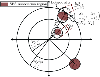
Figure 2: An illustration of association region.

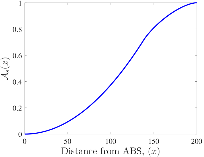
Figure 3: Variation of association probability to SBS with distance from ABS.

III-A Association Region and Association Probability

We first define the association region in the representative user hotspot as follows. Given the representative hotspot is centered at ${\bf x}$, the SBS association region is defined as: ${\cal S}_{\bf x}=\{{\bf x}+{\bf u}\in b({\bf x},R_{\rm s}):P_{\rm m}\|{\bf x}+{\bf u}\|^{-\alpha}<P_{\rm s}u^{-\alpha}\}$ and the ABS association area is $b({\bf x},R_{\rm s})\cap{\cal S}_{\bf x}^{c}$. In the following Proposition, we characterize the shape of ${\cal S}_{\bf x}$.

Proposition 1.

The SBS association region ${\cal S}_{\bf x}$ for the SBS at ${\bf x}$ can be written as: ${\cal S}_{\bf x}=$

$$\begin{cases}b\bigg{(}(1-k_{p}^{2})^{-1}{\bf x},\frac{k_{p}x}{1-k_{p}^{2}}\bigg{)},&0<x<\frac{k_{p}R_{\rm s}}{1+k_{p}},\\ b\bigg{(}(1-k_{p}^{2})^{-1}{\bf x},\frac{k_{p}x}{1-k_{p}^{2}}\bigg{)}\cap b({\bf x},R_{\rm s}),&\frac{k_{p}R_{\rm s}}{1+k_{p}}\leq x\leq\frac{k_{p}R_{\rm s}}{1-k_{p}},\\ b({\bf x},R_{\rm s}),&x>\frac{k_{p}R_{\rm s}}{1-k_{p}},\end{cases}$$ (8)

where $k_{p}=\bigg{(}\frac{P_{\rm s}}{P_{\rm m}}\bigg{)}^{1/\alpha}$.

Proof:

Let ${\bf x}=(X_{1},X_{2})$ be the Cartesian representation of ${\bf x}$. Let, ${\cal S}_{\bf x}=\{(X_{1}+t_{1},X_{2}+t_{2})\}$. Then, following the definition of ${\cal S}_{\bf x}$, $P_{\rm m}(t_{1}^{2}+t_{2}^{2})^{-\alpha/2}\leq P_{\rm s}((t_{1}-X_{1})^{2}+(t_{2}-X_{2})^{2})^{-\alpha/2}\Rightarrow\bigg{(}t_{1}-\frac{X_{1}}{1-k_{p}^{2}}\bigg{)}^{2}+\bigg{(}t_{2}-\frac{X_{2}}{1-k_{p}^{2}}\bigg{)}^{2}\leq\bigg{(}\frac{k_{p}x}{1-k_{p}^{2}}\bigg{)}^{2}$. Thus, $\{(t_{1},t_{2})\}=b((1-k_{p}^{2})^{-1}{\bf x},k_{p}x/(1-k_{p}^{2}))$. Since, ${\cal S}_{\bf x}$ can not spread beyond $b({\bf x},R_{\rm s})$, ${\cal S}_{\bf x}=b\bigg{(}(1-k_{p}^{2})^{-1}{\bf x},\frac{k_{p}x}{1-k_{p}^{2}}\bigg{)}\cap b({\bf x},R_{\rm s})$. When $0<x<\frac{k_{p}}{1+k_{p}}R_{\rm s}$, $b\bigg{(}(1-k_{p}^{2})^{-1}{\bf x},\frac{k_{p}x}{1-k_{p}^{2}}\bigg{)}\subset b({\bf x},R_{\rm s})$. Beyond this limit of $x$, a part of $b((1-k_{p}^{2})^{-1}{\bf x},k_{p}x/(1-k_{p}^{2}))$ lies outside of $b({\bf x},R_{\rm s})$. Finally, when $x>\frac{k_{p}}{1-k_{p}}R_{\rm s}$, $b((1-k_{p}^{2})^{-1}{\bf x},k_{p}x/(1-k_{p}^{2}))\supset b({\bf x},R_{\rm s})$. ∎

This formulation of ${\cal S}_{\bf x}$ is illustrated in Fig. 2. We now compute the SBS association probability as follows.

Lemma 1.

Conditioned on the fact that the user belongs to the hotspot at ${\bf x}$, the association probability to SBS is given by: ${\cal A}_{\rm s}({\bf x})={\cal A}_{\rm s}(x)=$

$$\int_{0}^{2\pi}\frac{\bigg{(}\min\big{(}R_{\rm s},x\frac{k_{p}(\sqrt{1-k_{p}^{2}.\sin^{2}\xi}+k_{p}\cos\xi)}{1-k_{p}^{2}}\big{)}\bigg{)}^{2}}{2\pi R_{\rm s}^{2}}{\rm d}\xi$$ (9)

$$=\begin{cases}\frac{k_{p}^{2}x^{2}}{(1-k_{p}^{2})^{2}R_{\rm s}^{2}}&\text{if }0<x<\frac{k_{p}}{1+k_{p}}R_{\rm s},\\ \frac{{\cal C}\big{(}R_{\rm s},\frac{k_{p}x}{1-k_{p}^{2}},\frac{k_{p}^{2}x}{1-k_{p}^{2}}\big{)}}{\pi R_{\rm s}^{2}}&\text{if }\frac{k_{p}}{1+k_{p}}R_{\rm s}\leq x\leq\frac{k_{p}}{1-k_{p}}R_{\rm s},\\ 1&\text{if }x>\frac{k_{p}}{1-k_{p}}R_{\rm s}\end{cases},$$ (10)

where

$${\cal C}(r_{1},r_{2},d)=r_{1}^{2}\tan^{-1}\bigg{(}\frac{t}{d^{2}+r_{1}^{2}-r_{2}^{2}}\bigg{)}\\ +r_{2}^{2}\tan^{-1}\bigg{(}\frac{t}{d^{2}-r_{1}^{2}+r_{2}^{2}}\bigg{)}-{\frac{t}{2}}$$

is the area of intersection of two intersecting circles of radii $r_{1}$, and $r_{2}$ and distance between centers $d$ with $t=(d+r_{1}+r_{2})^{\frac{1}{2}}(d+r_{1}-r_{2})^{\frac{1}{2}}(d-r_{1}+r_{2})^{\frac{1}{2}}(-d+r_{1}+r_{2})^{\frac{1}{2}}$. The association probability to the ABS is given by ${\cal A}_{\rm m}({x})=1-{\cal A}_{\rm s}({x})$.

Proof:

Conditioned on the location of the hotspot center at ${\bf x}$, ${\cal A}_{\rm s}({\bf x})={\mathbb{P}}({\cal E}=1|{\bf x})=$

$${\mathbb{E}}[{\bf 1}(P_{\rm m}\|{\bf x}+{\bf u}\|^{-\alpha}<P_{\rm s}\|{\bf u}\|^{-\alpha})|{\bf x}]={\mathbb{P}}({\bf x}+{\bf u}\in{\cal S}_{\bf x}|{\bf x})$$

$$={\mathbb{P}}(P_{\rm m}(x^{2}+u^{2}+2xu\cos\xi)^{-\alpha/2}<P_{\rm s}u^{-\alpha})|x)$$

$$={\mathbb{P}}(u^{2}(1-k_{p}^{2})-2x\cos\xi k_{p}^{2}u-k_{p}^{2}x^{2}<0|x)$$

$$\mathrel{\overset{\makebox[0.07pt]{\mbox{(a)}}}{=}}{\mathbb{P}}\bigg{(}u\in\bigg{(}0,\frac{xk_{p}\big{(}\sqrt{1-k_{p}^{2}\sin^{2}\xi}+k_{p}\cos\xi\big{)}}{1-k_{p}^{2}}\bigg{)},$$

$$\qquad\qquad\xi\in(0,2\pi]\bigg{|}x\bigg{)}$$

$$=\int_{0}^{2\pi}\int_{0}^{R_{\rm s}}{\bf 1}\bigg{(}0\leq u<\frac{xk_{p}\big{(}\sqrt{1-k_{p}^{2}\sin^{2}\xi}+k_{p}\cos\xi\big{)}}{1-k_{p}^{2}}\bigg{)}$$

$$\times f_{U}(u){\rm d}u\frac{1}{2\pi}{\rm d}{\xi},$$

where $\xi=\arg({\bf u}-{\bf x})$ and is uniformly distributed in $(0,2\pi]$. Here, (a) follows from solving the quadratic inequality inside the indicator function. The last step follows from deconditioning over ${u}$ and $\xi$. Finally, (9) is obtained by evaluating the integration over $u$. Note that, due to angular symmetry, ${\cal A}_{\rm s}({\bf x})={\cal A}_{\rm s}({x})$. Alternatively,

$${\cal A}_{\rm s}(x)=\int_{{\cal S}_{\bf x}}f_{U}(u){\rm d}u\frac{1}{2\pi}{\rm d}{\xi}=\frac{|{\cal S}_{\bf x}|}{\pi R_{\rm s}^{2}}.$$

The final result in (10) is obtained by using Proposition 1. ∎

In Fig. 3, we plot ${\cal A}_{\rm s}(x)$ as a function of $x$. We now evaluate the coverage probability of a typical user which is the probability of the occurrence of the events defined in (5).

Theorem 1.

The coverage probability is given by:

$$\mathtt{P_{c}}=\int\limits_{0}^{R-R_{\rm s}}\big{(}\mathtt{P_{c}}_{\rm s}(\theta_{1},\theta_{2}|x)+\mathtt{P_{c}}_{\rm m}(\theta_{3}|x)\big{)}f_{X}(x){\rm d}x,$$ (11)

where $\mathtt{P_{c}}_{\rm s}(\theta_{1},\theta_{2}|x)=$

$$\int\limits_{0}^{2\pi}\int\limits_{0}^{u_{\max}(x,\xi)}\bigg{(}p({x})F_{h}\bigg{(}\frac{x^{\alpha_{L}}\beta{\tt N}_{0}W\theta_{1}}{P_{\rm m}G^{2}},m_{L}\bigg{)}+(1-p({x}))\\ \times F_{h}\bigg{(}\frac{x^{\alpha_{NL}}\beta{\tt N}_{0}W\theta_{1}}{P_{\rm m}G^{2}},m_{NL}\bigg{)}\bigg{)}\bigg{(}p({u})F_{h}\bigg{(}\frac{u^{\alpha_{L}}\beta{\tt N}_{0}W\theta_{2}}{P_{\rm s}G},m_{L}\bigg{)}\\ +(1-p({u}))F_{h}\bigg{(}\frac{u^{\alpha_{NL}}\beta{\tt N}_{0}W\theta_{2}}{P_{\rm s}G},m_{NL}\bigg{)}\bigg{)}\frac{f_{U}(u)}{2\pi}{\rm d}{u}\>{\rm d}{\xi},$$

where $u_{\max}(x,\xi)=\min\bigg{(}R_{\rm s},xk_{p}\frac{\sqrt{(1-k_{p}^{2}\sin^{2}\xi)}+k_{p}\cos\xi)}{1-k_{p}^{2}}\bigg{)}$ and $F_{h}(\cdot)$ is the complementary cumulative distribution function (CCDF) of Gamma distribution, and $\mathtt{P_{c}}_{\rm m}(\theta_{3}|x)=$

$$\int\limits_{0}^{2\pi}\int\limits_{u_{\max}(x,\xi)}^{R_{\rm s}}{\bigg{(}p(\kappa(x,u,\xi))F_{h}\bigg{(}\frac{{\kappa(x,u,\xi)}^{\alpha_{L}}\beta{\tt N}_{0}W\theta_{3}}{P_{\rm m}G},m_{L}\bigg{)}}\\ +(1-p(\kappa(x,u,\xi)))F_{h}\bigg{(}\frac{{\kappa(x,u,\xi)}^{\alpha_{NL}}\beta{\tt N}_{0}W\theta_{3}}{P_{\rm m}G},m_{NL}\bigg{)}\bigg{)}\\ \times\frac{f_{U}(u){\rm d}u\>{\rm d}\xi}{2\pi},$$

where $\kappa(x,u,\xi)=({x^{2}+u^{2}+2xu\cos\xi})^{1/2}$.

Proof:

See Appendix -A. ∎

As expected, coverage probability is the summation of two terms, each corresponding to the probability of occurrences of the two mutually exclusive events appearing in (5).

III-B Load distributions

While the load distributions for the PPP-based models are well-understood [47, 38], they are not directly applicable to the 3GPP-inspired finite model used in this paper. Consequently, in this Section, we provide a novel approach to characterize the ABS and SBS load for this model. As we saw in (7c), the load on the ABS has two components, one is due to the contribution of the number of users of the representative hotspot connecting to the ABS (denoted by $N_{{\bf x}}^{\rm ABS}$) and the other is due to the macro users of the other clusters, which we lump into a single random variable, $N_{\rm o}^{\rm ABS}=\sum_{i=1}^{n-1}N_{{\bf x}_{i}}^{\rm ABS}$. On the other hand, $N_{\bf x}^{\rm SBS}$ and $N_{\rm o}^{\rm SBS}=\sum_{i=1}^{n-1}N_{{\bf x}_{i}}^{\rm SBS}$ respectively denote the load on the SBS at ${\bf x}$ and sum load of all SBSs except the one at ${\bf x}$. First, we obtain the PMFs of $N_{{\bf x}}^{\rm ABS}$ and $N_{{\bf x}}^{\rm SBS}$ using the fact that given the location of the representative hotspot centered at ${\bf x}$, each user belongings to the association regions ${\cal S}_{\bf x}$ or $b({\bf x},R_{\rm s})\cap{{\cal S}}_{\bf x}^{c}$ according to an i.i.d. Bernoulli random variable.

Lemma 2.

Given the fact that the representative hotspot is centered at ${\bf x}$, load on the ABS due to the macro users in the hotspot at ${\bf x}$ ($N^{\rm ABS}_{{\bf x}}$) and load on the SBS at $\bf x$ ($N^{\rm SBS}_{\bf x}$) are distributed as follows:

case $1$ ($N_{{\bf x}_{i}}=\bar{m}$, $\forall\ i=1,\dots,n$).

$${\mathbb{P}}(N^{\rm ABS}_{{\bf x}}=k|{\bf x})={\bar{m}-1\choose k-1}{\cal A}_{\rm m}(x)^{k-1}{\cal A}_{\rm s}(x)^{\bar{m}-k},$$ (12a)

$${\mathbb{P}}(N^{\rm SBS}_{{\bf x}}=k|{\bf x})={\bar{m}-1\choose k-1}{\cal A}_{\rm s}(x)^{k-1}{\cal A}_{\rm m}(x)^{\bar{m}-k},$$ (12b)

where $k=1,2,\dots,\bar{m}$.

case $2$ ($N_{{\bf x}_{i}}\stackrel{{\scriptstyle i.i.d.}}{{\sim}}{\tt Poisson}(\bar{m})$, $\forall\ i=1,\dots,n$).

$${\mathbb{P}}(N^{\rm ABS}_{{\bf x}}=k|{\bf x})=\frac{(\bar{m}{\cal A}_{\rm m}(x))^{k-1}}{(k-1)!}e^{-\bar{m}{\cal A}_{\rm m}(x)},$$ (13a)

$${\mathbb{P}}(N^{\rm SBS}_{{\bf x}}=k|{\bf x})=\frac{(\bar{m}{\cal A}_{\rm s}(x))^{k-1}}{(k-1)!}e^{-\bar{m}{\cal A}_{\rm s}(x)},$$ (13b)

where $k\in{\mathbb{Z}}^{+}$.

Proof:

See Appendix -B. ∎

We present the first moments of these two load variables in the following Corollary which will be required for the evaluation of the rate coverage for the average load-based partition and the derivation of easy-to-compute approximations of rate coverage in the sequel.

Corollary 1.

The conditional means of $N_{\bf x}^{\rm ABS}$ and $N_{\bf x}^{\rm SBS}$ given the center of the representative hotspot at $\bf x$ are

$$\text{{\sc case}~{}$1$: }{\mathbb{E}}[N_{\bf x}^{\rm ABS}]=(\bar{m}-1){\cal A}_{\rm m}(x)+1,{\mathbb{E}}[N_{\bf x}^{\rm SBS}]=$$

$$\qquad\qquad\qquad\qquad(\bar{m}-1){\cal A}_{\rm s}(x)+1,$$

$$\text{{\sc case}~{}$2$: }{\mathbb{E}}[N_{\bf x}^{\rm ABS}]=\bar{m}{\cal A}_{\rm m}(x)+1,{\mathbb{E}}[N_{\bf x}^{\rm SBS}]=\bar{m}{\cal A}_{\rm s}(x)+1.$$

We now obtain the PMFs of $N_{\rm o}^{\rm ABS}$ and $N_{\rm o}^{\rm SBS}$ in the following Lemma. Note that, since ${\bf x}_{i}$-s are i.i.d., $N_{\rm o}^{\rm ABS}$ and $N_{\rm o}^{\rm SBS}$ are independent of ${\bf x}$. In what follows, the exact PMF of $N_{{\rm o}}^{\rm ABS}$ ($N_{{\rm o}}^{\rm SBS}$) is in the form of $(n-1)$-fold discrete convolution and hence is not computationally efficient beyond very small values of $n$. We present an alternate easy-to-use expression of this PMF by invoking central limit theorem (CLT). In the numerical results Section, we verify that this approximation is tight even for moderate values of $n$.

Lemma 3.

Given the fact that the typical user belongs to a hotspot at ${\bf x}$, load on the ABS due to all other $n-1$ hotspots is distributed as: $\frac{N_{\rm o}^{\rm ABS}-\upsilon_{\rm m}}{\sigma_{\rm m}}\sim{\cal N}(0,1)\text{ (for large $n$)}$ and sum of the loads on the other SBSs at ${\bf x}_{1},{\bf x}_{2},\dots,{\bf x}_{n-1}$ is distributed as: $\frac{N_{\rm o}^{\rm SBS}-\upsilon_{\rm s}}{\sigma_{\rm s}}\sim{\cal N}(0,1)\text{ (for large $n$)}$, where ${\cal N}(0,1)$ denotes the standard normal distribution, $\upsilon_{\rm m}=(n-1)\bar{m}{\mathbb{E}}[{\cal A}_{\rm m}(X)],\upsilon_{\rm s}=(n-1)\bar{m}{\mathbb{E}}[{\cal A}_{\rm s}(X)],$ and

$$\text{for {\sc case}~{}$1$, }\sigma_{\rm m}^{2}=(n-1)\big{[}\bar{m}{\mathbb{E}}[{\cal A}_{\rm m}(X){\cal A}_{\rm s}(X)]$$

$$\qquad\qquad\qquad\quad+\bar{m}^{2}{\rm Var}[{\cal A}_{\rm m}(X)]\big{]}=\sigma_{\rm s}^{2},$$

$$\text{for {\sc case}~{}$2$, }\sigma_{\rm m}^{2}=(n-1)\big{[}\bar{m}{\mathbb{E}}[{\cal A}_{\rm m}(X)]+\bar{m}^{2}{\rm Var}[{\cal A}_{\rm m}(X)]\big{]},$$

$$\sigma_{\rm s}^{2}=(n-1)\big{[}\bar{m}{\mathbb{E}}[{\cal A}_{\rm s}(X)]+\bar{m}^{2}{\rm Var}[{\cal A}_{\rm s}(X)]\big{]}.$$

Here,

$${\mathbb{E}}[{\cal A}_{\rm m}(X)]=\int_{0}^{R-R_{\rm s}}{\cal A}_{\rm m}(x)f_{X}(x){\rm d}x,\text{ and }\\ {\rm Var}[{\cal A}_{\rm m}(X)]=\int\limits_{0}^{R-R_{\rm s}}\big{(}{\cal A}_{\rm m}(x)\big{)}^{2}f_{X}(x){\rm d}x-({\mathbb{E}}[{\cal A}_{\rm m}(X)])^{2},$$

and ${\mathbb{E}}[{\cal A}_{\rm s}(X)]$, ${\rm Var}[{\cal A}_{\rm s}(X)]$ can be similarly obtained by replacing ${\cal A}_{\rm m}(X)$ with ${\cal A}_{\rm s}(X)$ in the above expressions.

Proof:

See Appendix -C. ∎

III-C Rate Coverage Probability

We first define the downlink rate coverage probability (or simply, rate coverage) as follows.

Definition 1 (Rate coverage probability).

The rate coverage probability of a link with BW $\tilde{W}$ is defined as the probability that the maximum achievable data rate (${\cal R}$) exceeds a certain threshold $\rho$, i.e., ${\mathbb{P}}({\cal R}>\rho)=$

$${\mathbb{P}}\bigg{(}\tilde{W}\log_{2}(1+\mathtt{SNR})>\rho\bigg{)}={\mathbb{P}}(\mathtt{SNR}>2^{{\rho}/{\tilde{W}}}-1).$$ (14)

Hence, we see that the rate coverage probability is the coverage probability evaluated at a modified $\mathtt{SNR}$-threshold. We now evaluate the rate coverage probability for different backhaul BW partition strategies for a general distribution of $N_{{\bf x}_{i}}$ and $N_{{\bf x}}$ in the following Theorem. We later specialize this result for cases $1$ and $2$ for numerical evaluation.

Theorem 2.

The rate coverage probability for a target data rate $\rho$ is given by:

$$\mathtt{P_{r}}=\mathtt{P_{r}}_{\rm m}+\mathtt{P_{r}}_{\rm s},$$ (15)

where $\mathtt{P_{r}}_{\rm m}$ ($\mathtt{P_{r}}_{\rm s}$) denotes the ABS rate coverage (SBS rate coverage) which is the probability that the typical user is receiving data rate greater than or equal to $\rho$ and is served by the ABS (SBS). The ABS rate coverage is given by:

$$\mathtt{P_{r}}_{\rm m}=\int\limits_{-\infty}^{\infty}\int\limits_{0}^{R-R_{\rm s}}{\mathbb{E}}_{N_{\bf x}^{\rm ABS}}\bigg{[}\mathtt{P_{c}}_{\rm m}\bigg{(}2^{\frac{\rho(t+N_{\bf x}^{\rm ABS})}{W_{\rm a}}}-1|x\bigg{)}\bigg{]}\\ \times f_{X}(x){\rm d}x\frac{1}{\sigma_{\rm m}\sqrt{2\pi}}e^{-\frac{(t-\upsilon_{\rm m})^{2}}{2\sigma_{\rm m}^{2}}}{\rm d}t.$$ (16)

The SBS rate coverage depends on the backhaul BW partition strategy. For equal partition,

$$\mathtt{P_{r}}_{\rm s}=\int\limits_{0}^{R-R_{\rm s}}{\mathbb{E}}_{N_{\bf x}^{\rm SBS}}\bigg{[}\mathtt{P_{c}}_{\rm s}\bigg{(}2^{\frac{\rho nN^{\rm SBS}_{\bf x}}{W_{\rm b}}}-1,2^{\frac{\rho N^{\rm SBS}_{\bf x}}{W_{\rm a}}}-1\big{|}x\bigg{)}\bigg{]}f_{X}(x){\rm d}x,$$ (17)

for instantaneous load-based partition,

$$\mathtt{P_{r}}_{\rm s}=\int\limits_{-\infty}^{\infty}\int\limits_{0}^{R-R_{\rm s}}{\mathbb{E}}_{N_{\bf x}^{\rm SBS}}\bigg{[}\mathtt{P_{c}}_{\rm s}\bigg{(}2^{\frac{\rho(N^{\rm SBS}_{\bf x}+t)}{W_{\rm b}}}-1,2^{\frac{\rho N^{\rm SBS}_{\bf x}}{W_{\rm a}}}-1\big{|}x\bigg{)}\bigg{]}\\ \times f_{X}(x){\rm d}x\frac{1}{\sigma_{\rm s}\sqrt{2\pi}}e^{-\frac{(t-\upsilon_{\rm s})^{2}}{2\sigma_{\rm s}^{2}}}{\rm d}t,$$ (18)

and for average load-based partition,

$$\mathtt{P_{r}}_{\rm s}=\int\limits_{-\infty}^{\infty}\int\limits_{0}^{R-R_{\rm s}}{\mathbb{E}}_{N_{\bf x}^{\rm SBS}}\bigg{[}\mathtt{P_{c}}_{\rm s}\bigg{(}2^{\frac{\rho N^{\rm SBS}_{\bf x}\left({\mathbb{E}}[N_{\bf x}^{\rm SBS}]+\bar{m}t\right)}{W_{\rm b}{\mathbb{E}}[N_{\bf x}^{\rm SBS}]}}-1,\\ 2^{\frac{\rho N^{\rm SBS}_{\bf x}}{W_{\rm a}}}-1\big{|}x\bigg{)}\bigg{]}f_{X}(x){\rm d}x\frac{e^{-\frac{\big{(}t-(n-1){\mathbb{E}}[{\cal A}_{\rm s}(X)]\big{)}^{2}}{2(n-1){\rm Var}[{\cal A}_{\rm s}(X)]}}}{\sqrt{2\pi(n-1){\rm Var}[{\cal A}_{\rm s}(X)]}}{\rm d}t.$$ (19)

Proof:

See Appendix -D. ∎

Note that the key enabler of the expression of $\mathtt{P_{r}}$ in Theorem 2 is the fact that the system is considered to be noise-limited. Including the SBS interference into analysis is not straightforward from this point since it would involve coupling between the coverage probability and load since both are dependent on the locations of the other $n-1$ SBSs. Having derived the exact expressions of rate coverage in Theorem 2, we present approximations of these expressions by replacing (i) $N_{\bf x}^{\rm ABS}$ in $\mathtt{P_{r}}_{\rm m}$ with its mean ${\mathbb{E}}[N_{\bf x}^{\rm ABS}]$, and (ii) $N_{\bf x}^{\rm SBS}$ in $\mathtt{P_{r}}_{\rm s}$ with its mean ${\mathbb{E}}[N_{\bf x}^{\rm SBS}]$ in the following Lemma.

Lemma 4.

The ABS rate coverage can be approximated as

$$\mathtt{P_{r}}_{\rm m}=\int\limits_{-\infty}^{\infty}\int\limits_{0}^{R-R_{\rm s}}\mathtt{P_{c}}_{\rm m}\bigg{(}2^{\frac{\rho(t+{\mathbb{E}}[N_{\bf x}^{\rm ABS}])}{W_{\rm a}}}-1|x\bigg{)}f_{X}(x){\rm d}x\\ \times\frac{e^{-\frac{(t-\upsilon_{\rm m})^{2}}{2\sigma_{\rm m}^{2}}}}{\sigma_{\rm m}\sqrt{2\pi}}{\rm d}t.$$ (20)

The SBS rate coverage can be approximated as follows. For equal partition,

$$\mathtt{P_{r}}_{\rm s}=\int\limits_{0}^{R-R_{\rm s}}\mathtt{P_{c}}_{\rm s}\bigg{(}2^{\frac{\rho n{\mathbb{E}}[N^{\rm SBS}_{\bf x}]}{W_{\rm b}}}-1,2^{\frac{\rho{\mathbb{E}}[N^{\rm SBS}_{\bf x}]}{W_{\rm a}}}-1\big{|}x\bigg{)}f_{X}(x){\rm d}x,$$ (21)

for instantaneous load-based partition,

$$\mathtt{P_{r}}_{\rm s}=\int\limits_{-\infty}^{\infty}\int\limits_{0}^{R-R_{\rm s}}\mathtt{P_{c}}_{\rm s}\bigg{(}2^{\frac{\rho({\mathbb{E}}[N^{\rm SBS}_{\bf x}]+t)}{W_{\rm b}}}-1,2^{\frac{\rho{\mathbb{E}}[N^{\rm SBS}_{\bf x}]}{W_{\rm a}}}-1\big{|}x\bigg{)}\\ \times f_{X}(x){\rm d}x\frac{e^{-\frac{(t-\upsilon_{\rm s})^{2}}{2\sigma_{\rm s}^{2}}}}{\sigma_{\rm s}\sqrt{2\pi}}{\rm d}t,$$ (22)

and for average load-based partition,

$$\mathtt{P_{r}}_{\rm s}=\int\limits_{-\infty}^{\infty}\int\limits_{0}^{R-R_{\rm s}}\mathtt{P_{c}}_{\rm s}\bigg{(}2^{\frac{\rho\left({\mathbb{E}}[N_{\bf x}^{\rm SBS}]+\bar{m}t\right)}{W_{\rm b}}}-1,2^{\frac{\rho{\mathbb{E}}[N^{\rm SBS}_{\bf x}]}{W_{\rm a}}}-1\big{|}x\bigg{)}\\ \times f_{X}(x){\rm d}x\frac{e^{-\frac{\big{(}t-(n-1){\mathbb{E}}[{\cal A}_{\rm s}(X)]\big{)}^{2}}{2(n-1){\rm Var}[{\cal A}_{\rm s}(X)]}}}{\sqrt{2\pi(n-1){\rm Var}[{\cal A}_{\rm s}(X)]}}{\rm d}t.$$ (23)

TABLE I: Key system parameters

Notation	Parameter	Value
$P_{\rm m},\ P_{\rm s}$	BS transmit powers	50, 20 dBm
$\alpha_{L},\alpha_{NL}$	Path-loss exponent	2.0, 3.3
$\beta$	Path loss at 1 m	70 dB
$G$	Main lobe gain	18 dB
$\mu$	LOS range constant	170 m
${\tt N}_{0}W$	Noise power	-174 dBm/Hz+ $10\log_{10}W$ +10 dB (noise-figure)
$m_{L},m_{NL}$	Parameter of Nakagami distribution	2, 3
$R$, $R_{\rm s}$	Macrocell and hotspot radius	200 m, 30 m
$\bar{m}$	Average number of users per hotspot	5
$\rho$	Rate threshold	50 Mbps

We now specialize the result of Theorem 2 for cases $1$ and $2$ in the following Corollaries.

Corollary 2.

For case $1$, i.e., when $N_{{\bf x}_{i}}=\bar{m}$, $\forall\ i=1,\dots,n$, the ABS rate coverage is

$$\mathtt{P_{r}}_{\rm m}=\sum\limits_{k=1}^{\bar{m}}{{\bar{m}-1}\choose k-1}\int\limits_{-\infty}^{\infty}\int\limits_{0}^{R-R_{\rm s}}\mathtt{P_{c}}_{\rm m}\bigg{(}2^{\frac{\rho(t+k)}{W_{\rm a}}}-1|x\bigg{)}\\ \times{\cal A}_{\rm m}(x)^{k-1}{\cal A}_{\rm s}(x)^{\bar{m}-k}f_{X}(x){\rm d}x\frac{1}{\sigma_{\rm m}\sqrt{2\pi}}e^{-\frac{(t-\upsilon_{\rm m})^{2}}{2\sigma_{\rm m}^{2}}}{\rm d}t.$$ (24)

The SBS rate coverages for the three backhaul BW parition strategies are expressed as follows. (i) For equal partition,

$$\mathtt{P_{r}}_{\rm s}=\sum\limits_{k=1}^{\bar{m}}{{\bar{m}-1}\choose k-1}\int\limits_{0}^{R-R_{\rm s}}\mathtt{P_{c}}_{\rm s}\bigg{(}2^{\frac{\rho nk}{W_{\rm b}}}-1,2^{\frac{\rho k}{W_{\rm a}}}-1\big{|}x\bigg{)}\\ \times{\cal A}_{\rm s}(x)^{k-1}{\cal A}_{\rm m}(x)^{\bar{m}-k}f_{X}(x){\rm d}x,$$ (25)

(ii) for instantaneous load-based partition,

$$\mathtt{P_{r}}_{\rm s}=\sum\limits_{k=1}^{\bar{m}}{{\bar{m}-1}\choose k-1}\int\limits_{-\infty}^{\infty}\int\limits_{0}^{R-R_{\rm s}}\mathtt{P_{c}}_{\rm s}\bigg{(}2^{\frac{\rho(k+t)}{W_{\rm b}}}-1,2^{\frac{\rho k}{W_{\rm a}}}-1\big{|}x\bigg{)}\\ \times{\cal A}_{\rm s}(x)^{k-1}{\cal A}_{\rm m}(x)^{\bar{m}-k}f_{X}(x){\rm d}x\frac{e^{-\frac{(t-\upsilon_{\rm s})^{2}}{2\sigma_{\rm s}^{2}}}}{\sigma_{\rm s}\sqrt{2\pi}}{\rm d}t,$$ (26)

and (iii) for average load-based partition,

$$\mathtt{P_{r}}_{\rm s}=\sum\limits_{k=1}^{\bar{m}}{{\bar{m}-1}\choose k-1}\int\limits_{-\infty}^{\infty}\int\limits_{0}^{R-R_{\rm s}}\mathtt{P_{c}}_{\rm s}\bigg{(}2^{\frac{\rho k\left(1+(\bar{m}-1){\cal A}_{\rm s}(x)+\bar{m}t\right)}{W_{\rm b}(1+(\bar{m}-1){\cal A}_{\rm s}(x))}}-1,\\ 2^{\frac{\rho k}{W_{\rm a}}}-1\big{|}x\bigg{)}{\cal A}_{\rm s}(x)^{k-1}{\cal A}_{\rm m}(x)^{\bar{m}-k}\times f_{X}(x){\rm d}x\\ \times\frac{e^{-\frac{\big{(}t-(n-1){\mathbb{E}}[{\cal A}_{\rm s}(X)]\big{)}^{2}}{2(n-1){\rm Var}[{\cal A}_{\rm s}(X)]}}}{\sqrt{2\pi(n-1){\rm Var}[{\cal A}_{\rm s}(X)]}}{\rm d}t.$$ (27)

Proof:

The result can be obtained from Theorem 2 by using the PMFs of $N_{\bf x}^{\rm ABS}$, $N_{\bf x}^{\rm SBS}$, $N_{o}^{\rm ABS}$ and $N_{o}^{\rm ABS}$ from Lemmas 2 and 3 and substituting ${\mathbb{E}}[N_{\bf x}^{\rm SBS}]$ from Corollary 1 for case $1$. ∎

Corollary 3.

For case $2$, i.e., when $N_{{\bf x}_{i}}\stackrel{{\scriptstyle i.i.d.}}{{\sim}}{\tt Poisson}(\bar{m})$, $\forall\ i=1,\dots,n$, the ABS rate coverage is expressed as

$$\mathtt{P_{r}}_{\rm m}=\sum\limits_{k=1}^{\infty}\frac{\bar{m}^{k-1}}{(k-1)!}\int\limits_{-\infty}^{\infty}\int\limits_{0}^{R-R_{\rm s}}({\cal A}_{\rm m}(x))^{k-1}e^{-\bar{m}{\cal A}_{\rm m}(x)}\\ \times\mathtt{P_{c}}_{\rm m}\bigg{(}2^{\frac{\rho(t+k)}{W_{\rm a}}}-1|x\bigg{)}f_{X}(x){\rm d}x\frac{1}{\sigma_{\rm m}\sqrt{2\pi}}e^{-\frac{(t-\upsilon_{\rm m})^{2}}{2\sigma_{\rm m}^{2}}}{\rm d}t.$$ (28)

The SBS rate coverages for the three backhaul BW parition strategies are expressed as follows. (i) For equal partition,

$$\mathtt{P_{r}}_{\rm s}=\sum\limits_{k=1}^{\infty}\frac{\bar{m}^{k-1}}{(k-1)!}\int\limits_{0}^{R-R_{\rm s}}({\cal A}_{\rm s}(x))^{k-1}e^{-\bar{m}{\cal A}_{\rm s}(x)}\\ \times\mathtt{P_{c}}_{\rm s}\bigg{(}2^{\frac{\rho nk}{W_{\rm b}}}-1,2^{\frac{\rho k}{W_{\rm a}}}-1\big{|}x\bigg{)}f_{X}(x){\rm d}x,$$ (29)

(ii) for instantaneous load-based partition,

$$\mathtt{P_{r}}_{\rm s}=\sum\limits_{k=1}^{\infty}\frac{\bar{m}^{k-1}}{(k-1)!}\int\limits_{-\infty}^{\infty}\int\limits_{0}^{R-R_{\rm s}}({\cal A}_{\rm s}(x))^{k-1}e^{-\bar{m}{\cal A}_{\rm s}(x)}\\ \times\mathtt{P_{c}}_{\rm s}\bigg{(}2^{\frac{\rho(k+t)}{W_{\rm b}}}-1,2^{\frac{\rho k}{W_{\rm a}}}-1\big{|}x\bigg{)}f_{X}(x){\rm d}x\frac{1}{\sigma_{\rm s}\sqrt{2\pi}}e^{-\frac{(t-\upsilon_{\rm s})^{2}}{2\sigma_{\rm s}^{2}}}{\rm d}t,$$ (30)

and (iii) for average load-based partition,

$$\mathtt{P_{r}}_{\rm s}=\sum\limits_{k=1}^{\infty}\frac{\bar{m}^{k-1}}{(k-1)!}\int\limits_{-\infty}^{\infty}\int\limits_{0}^{R-R_{\rm s}}({\cal A}_{\rm s}(x))^{k-1}e^{-\bar{m}{\cal A}_{\rm s}(x)}\\ \times\mathtt{P_{c}}_{\rm s}\bigg{(}2^{\frac{\rho k\left(1+\bar{m}{\cal A}_{\rm s}(x)+\bar{m}t\right)}{W_{\rm b}(1+\bar{m}{\cal A}_{\rm s}(x))}}-1,2^{\frac{\rho k}{W_{\rm a}}}-1\big{|}x\bigg{)}\\ \times f_{X}(x){\rm d}x\frac{1}{\sqrt{2\pi(n-1){\rm Var}[{\cal A}_{\rm s}(X)]}}e^{-\frac{\big{(}t-(n-1){\mathbb{E}}[{\cal A}_{\rm s}(X)]\big{)}^{2}}{2(n-1){\rm Var}[{\cal A}_{\rm s}(X)]}}{\rm d}t.$$ (31)

Proof:

The result can be similarly obtained from Theorem 2 by using the PMFs of $N_{\bf x}^{\rm ABS}$, $N_{\bf x}^{\rm SBS}$, $N_{o}^{\rm ABS}$ and $N_{o}^{\rm ABS}$ from Lemmas 2 and 3, and substituting ${\mathbb{E}}[N_{\bf x}^{\rm SBS}]$ from Corollary 1 for case $2$. ∎

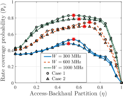
(a) Equal partition.

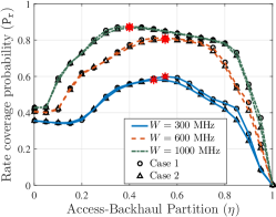
(b) Instantaneous load-based partition.

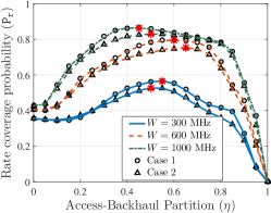
(c) Average load-based partition.

Figure 4: Rate coverage probability for different bandwidths for case $1$ and $2$ obtained by Corollaries 2 and 3 ($\rho=50$ Mbps, $n=10$). Lines and markers indicate theoretical and simulation results, respectively. Theoretical results for cases $1$ and $2$ are obtained from Corollaries 2 and 3, respectively.

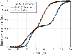
Figure 5: The CDF plot of SNR from the ABS and SBS ($P_{\rm m}=50$ dBm, $P_{\rm s}=20$ dBm). The markers indicate empirical CDF obtained from Monte Carlo simulations.

IV Results and Discussion

IV-A Trends of rate coverage

In this Section we verify the accuracy of our analysis of rate coverage with Monte Carlo simulations of the network model delineated in Section II with parameters listed in Table I. For each simulation, the number of iterations was set to $10^{6}$. Since $\mathtt{P_{r}}$ fundamentally depends upon $\mathtt{SNR}$, we first plot the cumulative density function (CDF) of SNRs without beamforming in Fig. 5, averaged over user locations. Precisely we plot ${\mathbb{E}}_{\bf x}\left[{\mathbb{P}}\left(\frac{h_{\rm m}P_{\rm m}\|{\bf x}\|^{-\alpha}}{{\tt N}_{0}W}<\theta\right)\right]=\int_{0}^{R-R_{\rm s}}\mathtt{P_{c}}_{\rm m}(\theta|x)f_{X}(x){\rm d}x$ and ${\mathbb{E}}_{\bf u}\left[{\mathbb{P}}\left(\frac{h_{\rm s}P_{\rm s}\|{\bf u}\|^{-\alpha}}{{\tt N}_{0}W}<\theta\right)\right]=\mathtt{P_{c}}_{\rm s}(-\infty,\theta|x)$, where $\mathtt{P_{c}}_{\rm m}$ and $\mathtt{P_{r}}_{\rm s}$ were defined in Theorem 1 from simulation and using our analytical results and observe a perfect match. We now plot the rate coverages for different user distributions (cases $1$ and $2$) for three different backhaul BW partition strategies in Figs. 4(a)-4(c). Recall that one part of ABS and SBS load was approximated using CLT in Lemma 3 for efficient computation. Yet, we obtain a perfect match between simulation and analysis even for $n=10$ for case $1$ and case $2$. Further, we observe that, (i) $\mathtt{P_{r}}=0$ for $\eta=1$ since this corresponds to the extreme when no BW is given to access links, and (ii) the rate coverage is maximized for a particular access-backhaul BW split ($\eta^{*}=\arg\max_{\{\eta\}}\mathtt{P_{r}}$). Also note that the rate coverage trends for cases $1$ and $2$ are the same, although $\mathtt{P_{r}}$ for case $1$ is slightly higher than $\mathtt{P_{r}}$ of case $2$ since the representative cluster, on average, has more number of users in case $2$ than in case $1$ (see Corollary 1). However, for space constraint, we only present the results of case $1$ for subsequent discussions.

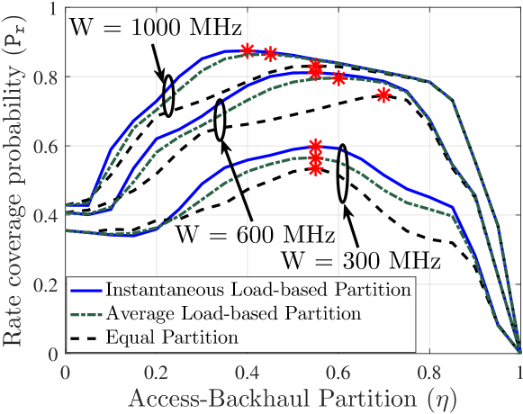
Figure 6: Comparison of backhaul partition strategies for case $1$ ($\rho=50$ Mbps, $n=10$).

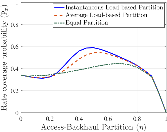
Figure 7: Comparision of backhaul BW parition strategies ($\rho=50$ Mbps, $n=10$, $W=600$ MHz) for case $1$ and $\mu=30$ m. The results are obtained from Corollary 2.

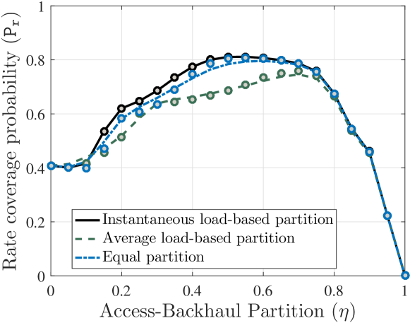
Figure 8: Comparison of the exact expression (Corollary 2) and approximate expression (Lemma 4) of rate coverage probability for case $1$ ($\rho=50$ Mbps, $W=600$ MHz, $n=10$). Lines and markers indicate exact and approximate results, respectively.

IV-A1 Comparison of backhaul BW partition strategies

In Fig. 6, we overlay $\mathtt{P_{r}}$ for three different backhaul BW partition strategies. We observe that the maximum rate coverage, $\mathtt{P_{r}}^{*}=\mathtt{P_{r}}(\eta^{*})$ (marked as ‘*’ in the figures) for instantaneous load-based partition dominates $\mathtt{P_{r}}^{*}$ in average load-based partition, and $\mathtt{P_{r}}^{*}$ in average load-based partition dominates $\mathtt{P_{r}}^{*}$ in equal partition. Also note that $\eta^{*}$ is different for different combination of BW partition strategy and $W$. We further compared these three strategies in a high blocking environment in Fig. 7 by setting $\mu=30$ m and observe the same ordering of performance of the three strategies. As expected, $\mathtt{P_{r}}$ is in general lower for this case. That said, it should be kept in mind that instantaneous load-based partition requires more frequent feedback of the load information from the SBSs and hence has the highest signaling overhead among the three strategies. The average load-based partition requires comparatively less signaling overhead since it does not require frequent feedback. On the other hand, equal partition does not have this overhead at all. This motivates an interesting performance-complexity trade-off for the design of cellular networks with IAB.

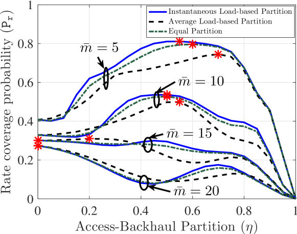
Figure 9: Rate coverage for different numbers of users per hotspot for case $1$ ($W=600$ MHz, $\rho=50$ Mbps). The values of $\mathtt{P_{r}}$ are computed using Lemma 4.

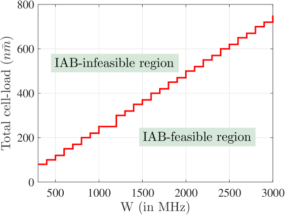
Figure 10: Total cell-load upto which IAB-enabled network outperforms macro-only network (for instantaneous load-based partition).

IV-A2 Effect of system BW

We observe the effect of increasing system BW on rate coverage in Fig 6. As expected, $\mathtt{P_{r}}$ increases as $W$ increases. However, the increment of $\mathtt{P_{r}}^{*}$ saturates for very high values of $W$ since high noise power degrades the link spectral efficiency. Another interesting observation is that starting from $\eta=0$ to $\eta^{*}$, $\mathtt{P_{r}}$ does not increase monotonically. This is due to the fact that sufficient BW needs to be steered from access to backhaul so that the network with IAB performs better than the macro-only network (corresponding to $\eta=0$).

IV-A3 Accuracy of approximation

We now plot $\mathtt{P_{r}}$ obtained by the approximations in Lemma 4 in Fig. 8. It is observed that the approximation is surprisingly close to the exact values of $\mathtt{P_{r}}$ obtained by Corollary 2. Motivated by the tightness of the approximation, we proceed with the easy-to-compute expressions of $\mathtt{P_{r}}$ obtained by Lemma 4 instead of the exact expressions (Corollary 2) for the metrics evaluated in the sequel, namely, critical load, median rate, and $5^{th}$ percentile rate. It is important to note that each numerical evaluation of these metrics requires high number of computations of $\mathtt{P_{r}}$ and is highly inefficient if $\mathtt{P_{r}}$ is computed by simulation, which further highlights the importance of analytical expressions derived in this paper.

IV-B Critical load

We plot the variation of $\mathtt{P_{r}}$ with $\bar{m}$ in Fig. 9. We observe that as $\bar{m}$ increases, more number of users share the BW and as a result, $\mathtt{P_{r}}$ decreases. However, the optimality of $\mathtt{P_{r}}$ completely disappears for very large value of $\bar{m}$ ($10<\bar{m}<20$ in this case). This implies that for given BW $W$ there exists a critical total cell-load ($n\bar{m}$) beyond which the gain obtained by the IAB architecture completely disappears. Observing Fig. 10, we find that the critical total cell-load varies linearly with the system BW. The reason of the existence of the critical total cell-load can be intuitively explained as follows. Recall that the SBS rate ${\cal R}_{\rm a}^{SBS}$ was limited by the backhaul constraint ${\cal R}_{\rm b}^{\rm ABS}/N_{\bf x}^{\rm SBS}$. When $\bar{m}$ is high, $N_{\bf x}^{\rm SBS}$ is also high and this puts stringent backhaul constraint on ${\cal R}_{\rm a}^{\rm SBS}$. Hence, an ABS can serve more users by direct macro-links at the target rate instead of allocating any backhaul partition.

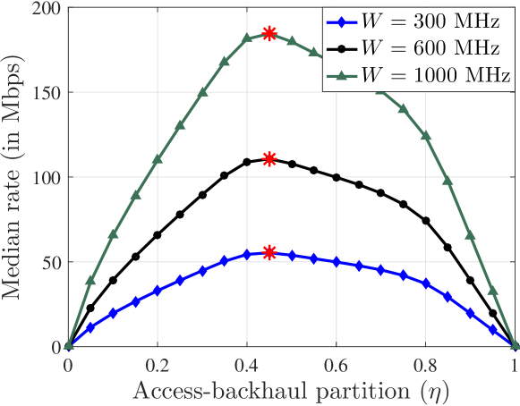
Figure 11: Median rate for case $1$ for instantaneous load-based partition ($n=10$).

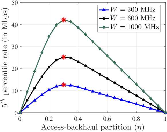
Figure 12: $5^{th}$ percentile rate for case $1$ for instantaneous load-based partition ($n=10$).

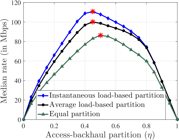
Figure 13: Median rate for case $1$ for different backhaul BW partition strategies ($n=10$, $W=600$ MHz).

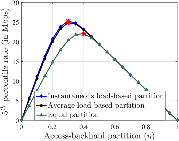
Figure 14: $5^{th}$ percentile rate for case $1$ for different backhaul BW partition strategies ($n=10$, $W=600$ MHz).

IV-C Median and $5^{th}$ percentile rates

We now shift our attention to two more performance metrics of interest, the median ($50^{th}$ percentile) and $5^{th}$ percentile rate, which are denoted as $\rho_{50}$ and $\rho_{95}$, respectively. These rates are defined as the values where the rate CDF attains $0.5$ and $0.05$, respectively, i.e., $\mathtt{P_{r}}=0.5$ at $\rho=\rho_{50}$ and $\mathtt{P_{r}}=0.95$ at $\rho=\rho_{95}$. Figs. 11 and 12 illustrate $\rho_{50}$ and $\rho_{95}$ respectively for different $W$. We first observe that for a given $\eta$, these rates increase linearly with $W$. This is because of the fact that in all the expressions of rate coverage, $\rho$ and $W$ appear as a ratio ($\rho/W$). Thus, once we find a desired rate coverage at a particular $\rho$ for a given $W$, same rate coverage will be observed for $kW$ at target data rate $k\rho$ (where $k$ is a positive constant). Further, we notice that the median rate is relatively flat around the maximum compared to the $5^{th}$ percentile rate. Also, the optimal $\eta$ does not vary significantly (stays close to 0.4 in our setup) for median and $5^{th}$ percentile rates. In Figs. 13 and 14, we have compared the three backhaul BW partition strategies in terms of these two rates. As expected, the ordering in performance is similar to the one observed for $\mathtt{P_{r}}^{*}$. Interestingly, from Fig. 14, it appears that the average and instantaneous load-based partition policies have almost similar performance in terms of $5^{th}$ percentile rate. This is because of the fact that $\rho_{95}$ is towards the tail of the rate distribution which is not significantly affected by difference between instantaneous or average load. However, the performance gap becomes prominent once median rate is considered.

V Conclusion

In this paper, we proposed the first 3GPP-inspired analytical framework for two-tier mm-wave HetNets with IAB and investigated three backhaul BW partition strategies. In particular, our model was inspired by the spatial configurations of the users and BSs considered in 3GPP simulation models of mm-wave IAB, where the SBSs are deployed at the centers of user hotspots. Under the assumption that the mm-wave communication is noise limited, we evaluated the downlink rate coverage probability. As a key intermediate step, we characterized the PMFs of load on the ABS and SBS for two different user distributions per hotspot. Our analysis leads to two important system-level insights: (i) for three performance metrics namely, downlink rate coverage probability, median rate, and $5^{th}$ percentile rate, the existence of the optimal access-backhaul bandwidth partition splits for which the metrics are maximized, and (ii) maximum total cell-load that can be supported using the IAB architecture.

This work has numerous extensions. From the modeling perspective, although the noise power dominates interference power in most of the operating regimes in mm-wave networks, it is important to consider interference from the ABS and the SBSs in the access links which may not be negligible in a very dense setup. For the analysis of rate coverage in this case, one needs to evaluate the joint distribution of interference and load which will be spatially coupled by the locations of the SBSs. Built on this baseline model of IAB, one can also study the spatial multiplexing gains on the resource allocation obtained by massive multi-user-multiple input-multiple-output (MU-MIMO) transmissions in the downlink. Further, this framework can be used to study IAB-enabled cellular networks where the control signalling for cell association is also performed in mm-wave. Under this setup, the problems of mm-wave beam sweeping and corresponding cell association delays can be studied. Another useful extension of this work is to consider an additional set of of users having open access to all the SBSs, while in this paper we only considered users with closed-access to the SBSs at the hotspot center. From the stochastic geometry perspective, it will be useful to develop analytical generative models for correlated blocking of the mm-wave signals making these analytical models more accurate. As said earlier, this work also lays the foundations of analytical characterization of cell-load in the 3GPP-inspired HetNet models. Using the fundamentals of this load modeling approach, one can further design optimal bias-factors depending on the volume of cell load at each hotspot and improve the per-user rates. Finally, the analysis can be extended to design delay sensitive routing/scheduling policies which is also a relevant research directions for IAB-enabled networks.

-A Proof of Theorem 1

Conditioned on the location of the typical user at ${\bf u}=(u,\xi)$ and its hotspot center at ${\bf x}$, $\mathtt{P_{c}}_{\rm s}(\theta_{1},\theta_{2}|{x})=$

$${\mathbb{P}}(\mathtt{SNR}^{\rm SBS}_{\rm a}({u})>\theta_{2},\mathtt{SNR}_{\rm b}({x})>\theta_{1},{\cal E}=1|x)=$$

$${\mathbb{P}}(\mathtt{SNR}^{\rm SBS}_{\rm a}({u})>\theta_{2},{\cal E}=1|x){\mathbb{P}}(\mathtt{SNR}_{\rm b}({x})>\theta_{1}|x)$$

$$\mathrel{\overset{\makebox[0.07pt]{\mbox{(a)}}}{=}}{\mathbb{E}}\bigg{[}\bigg{(}p({u}){\mathbb{P}}{\bigg{(}\frac{P_{\rm s}G\beta^{-1}h_{\rm s(L)}u^{-\alpha_{L}}}{{\tt N}_{0}W}>\theta_{2}\bigg{)}}$$

$$+(1-p({u})){\mathbb{P}}{\bigg{(}\frac{P_{\rm s}\beta^{-1}Gh_{\rm s(NL)}u^{-\alpha_{NL}}}{{\tt N}_{0}W}>\theta_{2}\bigg{)}}\bigg{)}\times$$

$${\bf 1}\bigg{(}u\in{\bigg{(}0,{\frac{xk_{p}\big{(}\sqrt{1-k_{p}^{2}\sin^{2}\xi}+k_{p}\cos\xi\big{)}}{1-k_{p}^{2}}}\bigg{)}},\xi\in(0,2\pi]\bigg{)}\bigg{|}x\bigg{]}$$

$$\times\bigg{(}p({x}){\mathbb{P}}\bigg{(}\frac{P_{\rm m}\beta^{-1}G^{2}h_{\rm b(L)}x^{-\alpha_{L}}}{{\tt N}_{0}W}>\theta_{1}|x\bigg{)}$$

$$+(1-p({x})){\mathbb{P}}\bigg{(}\frac{P_{\rm m}\beta^{-1}G^{2}h_{\rm b(NL)}x^{-\alpha_{NL}}}{{\tt N}_{0}W}>\theta_{1}|x\bigg{)}\bigg{)}.$$

Here (a) follows from step (a) in the proof of Lemma 1. The final form is obtained by evaluating the expectation with respect to $u$ and $\xi$. We can similarly obtain $\mathtt{P_{c}}_{\rm m}(\theta_{3}|{\bf x})=$

$${\mathbb{P}}(\mathtt{SNR}^{\rm ABS}_{\rm a}({{\bf x}+{\bf u}})>\theta_{3},{\cal E}=0|x)$$

$$={\mathbb{E}}\bigg{[}p(\sqrt{x^{2}+u^{2}+2xu\cos\xi})$$

$$\times{\mathbb{P}}{\bigg{(}\frac{P_{\rm m}G\beta^{-1}h_{\rm m(L)}(x^{2}+u^{2}+2xu\cos\xi)^{-\frac{\alpha_{L}}{2}}}{{\tt N}_{0}W}>\theta_{2}\bigg{)}}$$

$$+(1-p(\sqrt{x^{2}+u^{2}+2xu\cos\xi}))\times{\mathbb{P}}\bigg{(}\frac{P_{\rm m}\beta^{-1}Gh_{\rm m(NL)}}{{\tt N}_{0}W}$$

$$\times({x^{2}+u^{2}+2xu\cos\xi})^{-\frac{\alpha_{NL}}{2}}>\theta_{2}\bigg{)}\bigg{|}x\bigg{]},$$

followed by deconditioning over $u$ and $\xi$.

-B Proof of Lemma 2

Conditioned on the fact that the representative hotspot is centered at $\bf x$ and the typical user connects to the ABS, $N_{\bf x}^{\rm ABS}=1+N_{\bf x}^{\rm ABS,o}$, where $N_{\bf x}^{\rm ABS,o}$ is the load due to rest of the users in the representative hotspot connecting to the ABS, where, $N_{\bf x}^{\rm ABS,o}=$

$$\begin{cases}{\mathbb{E}}[\sum_{j=1}^{{N}_{\bf x}-1}\mathbf{1}({P_{\rm m}\|{\bf x}+{\bf u}_{j}\|^{-\alpha}>P_{\rm s}\|{\bf u}_{j}\|^{-\alpha}})|{\bf x}]&\\ &\text{for {\sc case}~{}$1$,}\\ {\mathbb{E}}[\sum_{j=1}^{{N}_{\bf x}}\mathbf{1}({P_{\rm m}\|{\bf x}+{\bf u}_{j}\|^{-\alpha}>P_{\rm s}\|{\bf u}_{j}\|^{-\alpha}})|{\bf x}]&\\ &\text{for {\sc case}~{}$2$.}\end{cases}$$

Note that the difference between the above two expressions is the upper bound of the summation. Recall that, $N_{\bf x}=N_{{\bf x}_{n}}=\bar{m}$ for case $1$, and $N_{\bf x}=N_{{\bf x}_{n}}+1$ for case $2$ (by Remark 1). Hence, the number of other users except the typical user in the representative cluster is $N_{\bf x}-1$ for case $1$ and $N_{\bf x}$ for case $2$. For case $1$, the conditional moment generating function (MGF) of $N_{\bf x}^{\rm ABS,o}$ is:

$${\mathbb{E}}[e^{sN_{\bf x}^{\rm ABS,o}}|{\bf x}]={\mathbb{E}}\bigg{[}\prod\limits_{j=1}^{\bar{m}-1}e^{s\mathbf{1}({P_{\rm m}\|{\bf x}+{\bf u}_{j}\|^{-\alpha}>P_{\rm s}\|{\bf u}_{j}\|^{-\alpha}})}|{\bf x}\bigg{]}$$

$$=\prod\limits_{j=1}^{\bar{m}-1}{\mathbb{E}}[e^{s\mathbf{1}({P_{\rm m}\|{\bf x}+{\bf u}_{j}\|^{-\alpha}>P_{\rm s}\|{\bf u}_{j}\|^{-\alpha}})}|{\bf x}]$$

$$=\prod\limits_{j=1}^{\bar{m}-1}e^{s}{\mathbb{P}}({P_{\rm m}\|{\bf x}+{\bf u}_{j}\|^{-\alpha}>P_{\rm s}\|{\bf u}_{j}\|^{-\alpha}}|{\bf x})$$

$$+{\mathbb{P}}(P_{\rm s}\|{\bf u}_{j}\|^{-\alpha}>P_{\rm m}\|{\bf x}+{\bf u}_{j}\|^{-\alpha}|{\bf x})$$

$$=({\cal A_{\rm m}}(x)e^{s}+(1-{\cal A_{\rm m}}(x)))^{\bar{m}-1},$$

which is the MGF of a Binomial distribution with $(\bar{m}-1,{\cal A}_{\rm m}(x))$. Here, the first step follows from the fact that ${\bf u}_{j}$-s are i.i.d. Similarly for case $2$,

$${\mathbb{E}}[e^{sN_{\bf x}^{\rm ABS,o}}|{\bf x}]={\mathbb{E}}\bigg{[}\prod\limits_{j=1}^{{N}_{{\bf x}}}{\mathbb{E}}[e^{s\mathbf{1}({P_{\rm m}\|{\bf x}+{\bf u}_{j}\|^{-\alpha}>P_{\rm s}\|{\bf u}_{j}\|^{-\alpha}})}|{\bf x}]\bigg{]}$$

$$={\mathbb{E}}[({\cal A_{\rm m}}(x)e^{s}+(1-{\cal A_{\rm m}}(x)))^{{N}_{\bf x}}]$$

$$=\sum_{k=0}^{\infty}({\cal A_{\rm m}}(x)e^{s}+(1-{\cal A_{\rm m}}(x)))^{k}\frac{\bar{m}^{k}e^{-\bar{m}}}{k!}=e^{\bar{m}{\cal A}_{\rm m}(x)(e^{s}-1)},$$

which is the MGF of a Poisson distribution with mean $\bar{m}{\cal A}_{\rm m}(x)$. From the PMF of $N_{\bf x}^{\rm ABS,o}$, one can easily obtain the PMF of $N_{\bf x}^{\rm ABS}$. The PMF of $N_{\bf x}^{\rm SBS}$ can be obtained on similar lines by altering the inequality in the first step of the above derivation.

-C Proof of Lemma 3

Following the proof of Lemma 2, conditioned on the location of a hotspot at ${\bf x}_{i}$, $N_{{\bf x}_{i}}^{\rm ABS}$ becomes (i) case $1$. a Binomial random variable with $(\bar{m},{{\cal A}}_{\rm m}({x}_{i}))$, or (ii) case $2$. a Poisson random variable with $\bar{m}{\cal A}_{\rm m}(x_{i})$. Now, $N_{\rm o}^{\rm ABS}=\sum_{i=1}^{n-1}{\mathbb{E}}_{{\bf x}_{i}}[N_{{\bf x}_{i}}^{\rm ABS}]$, where ${\mathbb{E}}_{{\bf x}_{i}}[N_{{\bf x}_{i}}^{\rm ABS}]$-s are i.i.d. with ${\mathbb{P}}({\mathbb{E}}_{{\bf x}_{i}}[N_{{\bf x}_{i}}^{\rm ABS}]=k)=$

$$\begin{cases}\int_{0}^{R-R_{\rm s}}{\bar{m}\choose k}{\cal A}_{\rm m}(x_{i})^{k}{\cal A}_{\rm s}(x_{i})^{\bar{m}-k}f_{X}(x_{i}){\rm d}{x_{i}},&\text{for {\sc case}~{}$1$}\\ \int_{0}^{R-R_{\rm s}}\frac{e^{-\bar{m}{\cal A}_{\rm m}(x_{i})}(\bar{m}{\cal A}_{\rm m}(x_{i}))^{k}}{k!}f_{X}(x_{i}){\rm d}x_{i},&\text{for {\sc case}~{}$2$}\end{cases},$$

where $k\in{\mathbb{Z}}^{+}$. The exact PMF of $N_{\rm o}^{\rm ABS}$ is obtained by the $(n-1)$-fold discrete convolution of this PMF. We avoid this complexity of the exact analysis by first characterizing the mean and variance of $N_{\rm o}^{\rm ABS}$ as: $\upsilon_{\rm m}={\mathbb{E}}[N_{\rm o}^{\rm ABS}]=\sum_{i=1}^{n-1}{\mathbb{E}}[{\mathbb{E}}_{{\bf x}_{i}}[N_{{\bf x}_{i}}^{\rm ABS}]]=(n-1)\bar{m}{\cal A}_{\rm m}(X)$, and $\sigma_{\rm m}^{2}=$

$${\rm Var}[N_{\rm o}^{\rm ABS}]\mathrel{\overset{\makebox[0.07pt]{\mbox{(a)}}}{=}}\sum_{i=1}^{n-1}{\rm Var}[{\mathbb{E}}_{{\bf x}_{i}}[N_{{\bf x}_{i}}^{\rm ABS}]]$$

$$=\sum_{i=1}^{n-1}{\mathbb{E}}[({\mathbb{E}}_{{\bf x}_{i}}[N_{{\bf x}_{i}}^{\rm ABS}])^{2}]-({\mathbb{E}}[{\mathbb{E}}_{{\bf x}_{i}}[N_{{\bf x}_{i}}^{\rm ABS}]])^{2}$$

$$=\begin{cases}\sum_{i=1}^{n-1}\int_{0}^{R-R_{\rm s}}(\bar{m}{\cal A}_{\rm m}(x_{i}){\cal A}_{\rm s}(x_{i})+(\bar{m}{\cal A}_{\rm m}(x_{i}))^{2})&\\ f_{X}(x_{i}){\rm d}{x_{i}}-(\bar{m}{\mathbb{E}}[{\cal A}_{\rm m}(X)])^{2},\text{ for {\sc case}~{}$1$}\\ \sum_{i=1}^{n-1}\int_{0}^{R-R_{\rm s}}(\bar{m}{\cal A}_{\rm m}(x_{i})+(\bar{m}{\cal A}_{\rm m}(x_{i}))^{2})f_{X}(x_{i}){\rm d}x_{i}\\ -(\bar{m}{\mathbb{E}}[{\cal A}_{\rm m}(X)])^{2},\text{ for {\sc case}~{}$2$}\end{cases},$$

where (a) is due to the fact that ${\mathbb{E}}_{{\bf x}_{i}}[N_{{\bf x}_{i}}^{\rm ABS}]$-s are i.i.d. The final result follows from some algebraic manipulation. Having derived the mean and variance of $N_{\rm o}^{\rm ABS}$, we invoke CLT to approximate the distribution of $N_{\rm o}^{\rm ABS}$ since it can be represented as a sum of i.i.d. random varables with finite mean and variance. Similar steps can be followed for the distribution of $N_{\rm o}^{\rm SBS}$.

-D Proof of Theorem 2

First we evaluate $\mathtt{P_{r}}_{\rm m}=\mathtt{P_{r}}_{\rm m}={\mathbb{P}}({\cal R}_{\rm a}^{\rm ABS}>\rho)=$

$${\mathbb{P}}\bigg{(}\frac{W_{\rm a}}{N_{\bf x}^{\rm ABS}+N_{\rm o}^{\rm ABS}}\log_{2}(1+\mathtt{SNR}_{\rm a}^{\rm ABS}({\bf x}+{\bf u}))>\rho\bigg{)}$$

$$={\mathbb{P}}\bigg{(}\mathtt{SNR}_{\rm a}^{\rm ABS}({\bf x}+{\bf u})>2^{\frac{\rho(N_{\bf x}^{\rm ABS}+N_{\rm o}^{\rm ABS})}{W_{\rm a}}}-1\bigg{)}$$

$$=\mathtt{P_{c}}_{\rm m}{\bigg{(}2^{\frac{\rho(N_{\bf x}^{\rm ABS}+N_{\rm o}^{\rm ABS})}{W_{\rm a}}}-1\bigg{)}},$$

where, the first step follows from (7c). The final form is obtained by deconditioning with respect to $N_{\bf x}^{\rm ABS}$, $N_{\rm o}^{\rm ABS}$ and $\bf x$. Now for equal partition, $\mathtt{P_{r}}_{\rm s}={\mathbb{P}}({\cal R}_{\rm a}^{\rm SBS}>\rho)=$

$${\mathbb{P}}\bigg{(}\frac{W_{\rm b}}{N_{\bf x}^{\rm SBS}n}\log_{2}(1+\mathtt{SNR}_{\rm b}({\bf x}))>\rho\bigg{)}$$

$$\qquad\times{\mathbb{P}}\bigg{(}\frac{W_{\rm a}}{N_{\bf x}^{\rm SBS}}\log_{2}(1+\mathtt{SNR}_{\rm a}^{\rm SBS}({\bf u}))>\rho\bigg{)}$$

$$={\mathbb{P}}\bigg{(}\mathtt{SNR}_{\rm b}({\bf x})>2^{\frac{\rho nN_{\bf x}^{\rm SBS}}{W_{\rm b}}}-1\bigg{)}{\mathbb{P}}\bigg{(}\mathtt{SNR}_{\rm a}^{\rm SBS}({\bf u})>2^{\frac{\rho N_{\bf x}^{\rm SBS}}{W_{\rm a}}}-1\bigg{)}$$

$$={\mathbb{E}}\bigg{[}\mathtt{P_{c}}_{\rm s}\bigg{(}2^{\frac{\rho nN_{\bf x}^{\rm SBS}}{W_{\rm b}}}-1,2^{\frac{\rho N_{\bf x}^{\rm SBS}}{W_{\rm a}}}-1\big{|}x\bigg{)}\bigg{]}.$$

Here step (a) follows from (7b) and the fact that the two rate terms appearing under the $\min$ operator are independent. The final form is obtained by deconditioning with respect to $N_{\bf x}^{\rm SBS}$ and $x$. For instantaneous load-based partition,

$$\mathtt{P_{r}}_{\rm s}={\mathbb{P}}\bigg{(}\frac{W_{\rm b}}{N_{\bf x}^{\rm SBS}+N_{\rm o}^{\rm SBS}}\log_{2}(1+\mathtt{SNR}_{\rm b}({\bf x}))>\rho\bigg{)}\\ \times{\mathbb{P}}\bigg{(}\frac{W_{\rm a}}{N_{\bf x}^{\rm SBS}}\log_{2}(1+\mathtt{SNR}^{\rm SBS}_{\rm a}({\bf u}))>\rho\bigg{)}\\ ={\mathbb{P}}\bigg{(}\mathtt{SNR}_{\rm b}({\bf x})>2^{\frac{\rho(N_{\bf x}^{\rm SBS}+N_{\rm o}^{\rm SBS})}{W_{\rm b}}}-1\bigg{)}\\ \times{\mathbb{P}}\bigg{(}\mathtt{SNR}_{\rm a}^{\rm SBS}({\bf u})>2^{\frac{\rho N_{\bf x}^{\rm SBS}}{W_{\rm a}}}-1\bigg{)}\\ ={\mathbb{E}}\bigg{[}\mathtt{P_{c}}_{\rm s}\bigg{(}2^{\frac{\rho(N_{\bf x}^{\rm SBS}+N_{\rm o}^{\rm SBS})}{W_{\rm b}}}-1,2^{\frac{\rho N_{\bf x}^{\rm SBS}}{W_{\rm a}}}-1\big{|}x\bigg{)}\bigg{]}.$$ (32)

The final form is obtained by deconditioning with respect to $N_{\bf x}^{\rm SBS}$, $N_{\rm o}^{\rm SBS}$ and $x$. For average load-based partition, $\mathtt{P_{r}}_{\rm s}=$

$${\mathbb{P}}\bigg{(}\frac{W_{\rm b}{\mathbb{E}}[N_{\bf x}^{\rm SBS}]}{N_{\bf x}^{\rm SBS}({\mathbb{E}}[N_{\bf x}^{\rm SBS}]+\sum_{i=1}^{n-1}{\mathbb{E}}[N_{{\bf x}_{i}}^{\rm SBS}])}\log_{2}(1+\mathtt{SNR}_{\rm b}({\bf x}))\\ >\rho\bigg{)}{\mathbb{P}}\bigg{(}\frac{W_{\rm a}}{N_{\bf x}^{\rm SBS}}\log_{2}(1+\mathtt{SNR}_{\rm a}^{\rm SBS}({\bf u}))>\rho\bigg{)}\\ ={\mathbb{P}}\bigg{(}\frac{W_{\rm b}{\mathbb{E}}[N_{\bf x}^{\rm SBS}]}{N_{\bf x}^{\rm SBS}({\mathbb{E}}[N_{\bf x}^{\rm SBS}]+\bar{m}\sum_{i=1}^{n-1}{\cal A}_{\rm s}(x_{i}))}\log_{2}(1+\mathtt{SNR}_{\rm b}({\bf x}))\\ >\rho\bigg{)}{\mathbb{P}}\bigg{(}\frac{W_{\rm a}}{N_{\bf x}^{\rm SBS}}\log_{2}(1+\mathtt{SNR}_{\rm a}^{\rm SBS}({\bf u}))>\rho\bigg{)},$$

where the last step is obtained by using the fact that ${\mathbb{E}}[N_{\bf x_{i}}^{\rm SBS}]=\bar{m}{\mathbb{E}}[{\cal A}_{\rm s}(X)]$ and ${\mathbb{E}}[N_{\bf x}^{\rm SBS}]$ depends on the underlying distribution of $N_{\bf x}$. Since the random variable $\sum_{i=1}^{n-1}{\cal A}_{\rm s}(x_{i})$ is a summation of $n-1$ i.i.d. random variables with mean $(n-1){\mathbb{E}}[{\cal A}_{\rm s}(X)]$ and variance $(n-1){\rm Var}[{\cal A}_{\rm s}(X)]$, we again invoke CLT instead of resorting to the exact expression that would have involved the $(n-1)$-fold convolution of the PDF of ${\cal A}_{\rm s}(X)$.

References

- [1] C. Saha, M. Afshang, and H. S. Dhillon, “Integrated mmwave access and backhaul in 5G: Bandwidth partitioning and downlink analysis,” in Proc., IEEE Int. Conf. Commun. (ICC), May 2018.
- [2] C. Dehos, J. L. González, A. De Domenico, D. Ktenas, and L. Dussopt, “Millimeter-wave access and backhauling: the solution to the exponential data traffic increase in 5G mobile communications systems?” IEEE Commun. Magazine, vol. 52, no. 9, pp. 88–95, 2014.
- [3] T. Q. S. Quek, G. de la Roche, I. Gven, and M. Kountouris, Small Cell Networks: Deployment, PHY Techniques, and Resource Management. New York, NY, USA: Cambridge University Press, 2013.
- [4] O. Tipmongkolsilp, S. Zaghloul, and A. Jukan, “The evolution of cellular backhaul technologies: Current issues and future trends,” IEEE Commun. Surveys Tuts., vol. 13, no. 1, pp. 97–113, 2011.
- [5] H. S. Dhillon and G. Caire, “Wireless backhaul networks: Capacity bound, scalability analysis and design guidelines,” IEEE Trans. on Wireless Commun., vol. 14, no. 11, pp. 6043–6056, Nov. 2015.
- [6] S. Rangan, T. S. Rappaport, and E. Erkip, “Millimeter-wave cellular wireless networks: Potentials and challenges,” Proc. IEEE, vol. 102, no. 3, pp. 366–385, Mar. 2014.
- [7] A. Ghosh, T. A. Thomas, M. C. Cudak, R. Ratasuk, P. Moorut, F. W. Vook, T. S. Rappaport, G. R. MacCartney, S. Sun, and S. Nie, “Millimeter-wave enhanced local area systems: A high-data-rate approach for future wireless networks,” IEEE Journal on Sel. Areas Commun., vol. 32, no. 6, pp. 1152–1163, Jun. 2014.
- [8] Z. Gao, L. Dai, D. Mi, Z. Wang, M. A. Imran, and M. Z. Shakir, “MmWave massive-MIMO-based wireless backhaul for the 5G ultra-dense network,” IEEE Wireless Commun., vol. 22, no. 5, pp. 13–21, Oct. 2015.
- [9] E. Dahlman, G. Mildh, S. Parkvall, J. Peisa, J. Sachs, Y. Selén, and J. Sköld, “5G wireless access: requirements and realization,” IEEE Commun. Magazine, vol. 52, no. 12, pp. 42–47, Dec. 2014.
- [10] 3GPP TR 38.874, “NR; Study on integrated access and backhaul,” Tech. Rep., 2017.
- [11] M. Haenggi, Stochastic Geometry for Wireless Networks. Cambridge University Press, 2012.
- [12] J. Andrews, F. Baccelli, and R. Ganti, “A tractable approach to coverage and rate in cellular networks,” IEEE Trans. on Commun., vol. 59, no. 11, pp. 3122–3134, 2011.
- [13] H. S. Dhillon, R. K. Ganti, F. Baccelli, and J. G. Andrews, “Modeling and analysis of -tier downlink heterogeneous cellular networks,” IEEE Journal on Sel. Areas in Commun., vol. 30, no. 3, pp. 550–560, Apr. 2012.
- [14] S. Mukherjee, “Distribution of downlink SINR in heterogeneous cellular networks,” IEEE Journal on Sel. Areas in Commun., vol. 30, no. 3, pp. 575–585, Apr. 2012.
- [15] P. Madhusudhanan, J. G. Restrepo, Y. Liu, and T. X. Brown, “Downlink coverage analysis in a heterogeneous cellular network,” in Proc., IEEE Globecom, Dec. 2012, pp. 4170–4175.
- [16] H. S. Jo, Y. J. Sang, P. Xia, and J. G. Andrews, “Heterogeneous cellular networks with flexible cell association: A comprehensive downlink SINR analysis,” IEEE Trans. on Wireless Commun., vol. 11, no. 10, pp. 3484–3495, Oct. 2012.
- [17] H. Elsawy, E. Hossain, and M. Haenggi, “Stochastic geometry for modeling, analysis, and design of multi-tier and cognitive cellular wireless networks: A survey,” IEEE Commun. Surveys Tuts., vol. 15, no. 3, pp. 996–1019, 3th quarter 2013.
- [18] H. ElSawy, A. Sultan-Salem, M. S. Alouini, and M. Z. Win, “Modeling and analysis of cellular networks using stochastic geometry: A tutorial,” IEEE Commun. Surveys Tuts., vol. 19, no. 1, pp. 167–203, Firstquarter 2017.
- [19] J. G. Andrews, A. K. Gupta, and H. S. Dhillon, “A primer on cellular network analysis using stochastic geometry,” 2016, available online: arxiv.org/abs/1604.03183.
- [20] S. Mukherjee, Analytical Modeling of Heterogeneous Cellular Networks. Cambridge University Press, 2014.
- [21] J. G. Andrews, T. Bai, M. N. Kulkarni, A. Alkhateeb, A. K. Gupta, and R. W. Heath, “Modeling and analyzing millimeter wave cellular systems,” IEEE Trans. Commun., vol. 65, no. 1, pp. 403–430, Jan. 2017.
- [22] M. D. Renzo, “Stochastic geometry modeling and analysis of multi-tier millimeter wave cellular networks,” IEEE Trans. on Wireless Commun., vol. 14, no. 9, pp. 5038–5057, Sep. 2015.
- [23] T. Bai and R. W. Heath, “Coverage and rate analysis for millimeter-wave cellular networks,” IEEE Trans. on Wireless Commun., vol. 14, no. 2, pp. 1100–1114, Feb. 2015.
- [24] E. Turgut and M. C. Gursoy, “Coverage in heterogeneous downlink millimeter wave cellular networks,” IEEE Trans. on Commun., vol. 65, no. 10, pp. 4463–4477, Oct. 2017.
- [25] S. Singh, M. N. Kulkarni, and J. G. Andrews, “A tractable model for rate in noise limited mmwave cellular networks,” in Proc. IEEE Asilomar, Nov. 2014, pp. 1911–1915.
- [26] Y. Li, F. Baccelli, J. G. Andrews, and J. C. Zhang, “Directional cell search delay analysis for cellular networks with static users,” IEEE Trans. on Commun., 2018, to appear.
- [27] A. Alkhateeb, Y. H. Nam, M. S. Rahman, J. Zhang, and R. W. Heath, “Initial beam association in millimeter wave cellular systems: Analysis and design insights,” IEEE Trans. Wireless Commun., vol. 16, no. 5, pp. 2807–2821, May 2017.
- [28] H. Elshaer, M. N. Kulkarni, F. Boccardi, J. G. Andrews, and M. Dohler, “Downlink and uplink cell association with traditional macrocells and millimeter wave small cells,” IEEE Trans. Wireless Commun., vol. 15, no. 9, pp. 6244–6258, Sep. 2016.
- [29] H. Raza, “A brief survey of radio access network backhaul evolution: part I,” IEEE Commun. Magazine, vol. 49, no. 6, pp. 164–171, Jun. 2011.
- [30] 3GPP TR 36.116, “Evolved universal terrestrial radio access (E-UTRA); Relay radio transmission and reception,” Tech. Rep., Mar. 2017.
- [31] 3GPP TR 36.117, “Evolved universal terrestrial radio access (E-UTRA); Relay conformance testing,” Tech. Rep., Mar. 2017.
- [32] N. Johansson, J. Lundsjö, G. Mildh, A. Ràcz, and C. Hoymann, “Self-backhauling in LTE,” U.S. Patent 8 797 952, Aug. 5, 2014.
- [33] MiWaveS, “Heterogeneous wireless network with millimetre wave small cell access and backhauling,” white paper, Jan. 2016, availabe online: https://goo.gl/vQENZM.
- [34] A. D. La Oliva, X. C. Perez, A. Azcorra, A. D. Giglio, F. Cavaliere, D. Tiegelbekkers, J. Lessmann, T. Haustein, A. Mourad, and P. Iovanna, “Xhaul: toward an integrated fronthaul/backhaul architecture in 5G networks,” IEEE Wireless Commun., vol. 22, no. 5, pp. 32–40, Oct. 2015.
- [35] G. Zhang, T. Q. S. Quek, M. Kountouris, A. Huang, and H. Shan, “Fundamentals of heterogeneous backhaul design–Analysis and optimization,” IEEE Trans. on Commun., vol. 64, no. 2, pp. 876–889, Feb. 2016.
- [36] V. Suryaprakash and G. P. Fettweis, “An analysis of backhaul costs of radio access networks using stochastic geometry,” in Proc. IEEE Int. Conf. Commun. (ICC). IEEE, Jun. 2014, pp. 1035–1041.
- [37] S. Singh and J. G. Andrews, “Joint resource partitioning and offloading in heterogeneous cellular networks,” IEEE Trans. on Wireless Commun., vol. 13, no. 2, pp. 888–901, Feb. 2014.
- [38] S. Singh, M. N. Kulkarni, A. Ghosh, and J. G. Andrews, “Tractable model for rate in self-backhauled millimeter wave cellular networks,” IEEE Journal on Sel. Areas in Commun., vol. 33, no. 10, pp. 2196–2211, Oct. 2015.
- [39] A. Sharma, R. K. Ganti, and J. K. Milleth, “Joint backhaul-access analysis of full duplex self-backhauling heterogeneous networks,” IEEE Trans. on Wireless Commun., vol. 16, no. 3, pp. 1727–1740, Mar. 2017.
- [40] H. Tabassum, A. H. Sakr, and E. Hossain, “Analysis of massive MIMO-enabled downlink wireless backhauling for full-duplex small cells,” IEEE Trans. on Commun., vol. 64, no. 6, pp. 2354–2369, Jun. 2016.
- [41] C. Saha, M. Afshang, and H. S. Dhillon, “Enriched -Tier HetNet model to enable the analysis of user-centric small cell deployments,” IEEE Trans. on Wireless Commun., vol. 16, no. 3, pp. 1593–1608, Mar. 2017.
- [42] ——, “3GPP-inspired HetNet model using poisson cluster process: Sum-product functionals and downlink coverage,” IEEE Trans. on Commun., vol. 66, no. 5, pp. 2219–2234, May 2018.
- [43] J. Qin, Examples and Basic Theories for Length Biased Sampling Problems. Springer Singapore, 2017, pp. 1–9.
- [44] 3GPP TR 36.872 V12.1.0 , “3rd generation partnership project; technical specification group radio access network; small cell enhancements for E-UTRA and E-UTRAN - physical layer aspects (release 12),” Tech. Rep., Dec. 2013.
- [45] T. Bai, R. Vaze, and R. W. Heath, “Analysis of blockage effects on urban cellular networks,” IEEE Trans. on Wireless Commun., vol. 13, no. 9, pp. 5070–5083, Sep. 2014.
- [46] 3GPP TR 36.814, “Further advancements for E-UTRA physical layer aspects,” Tech. Rep., 2010.
- [47] S. Singh, H. S. Dhillon, and J. G. Andrews, “Offloading in heterogeneous networks: Modeling, analysis, and design insights,” IEEE Trans. on Wireless Commun., vol. 12, no. 5, pp. 2484–2497, May. 2013.