Diffusion Maps meet Nyström

Abstract

Diffusion maps are an emerging data-driven technique for non-linear dimensionality reduction, which are especially useful for the analysis of coherent structures and nonlinear embeddings of dynamical systems. However, the computational complexity of the diffusion maps algorithm scales with the number of observations. Thus, long time-series data presents a significant challenge for fast and efficient embedding. We propose integrating the Nyström method with diffusion maps in order to ease the computational demand. We achieve a speedup of roughly two to four times when approximating the dominant diffusion map components.

Index Terms—  Dimension Reduction, Nyström method

1 Motivation

In the era of ‘big data’, dimension reduction is critical for data science. The aim is to map a set of high-dimensional points $x_{1},x_{2},...,x_{n}\in\mathcal{X}$ to a lower dimensional (feature) space $\mathcal{F}$

$$\Psi:\mathcal{X}\subseteq\mathbb{R}^{p}\rightarrow\mathcal{F}\subseteq\mathbb{R}^{d},\qquad d\ll p.$$

The map $\Psi$ aims to preserve large scale features, while suppressing uninformative variance (fine scale features) in the data [1, 2]. Diffusion maps provide a flexible and data-driven framework for non-linear dimensionality reduction [3, 4, 5, 6, 7]. Inspired by stochastic dynamical systems, diffusion maps have been used in a diverse set of applications including face recognition [8], image segmentation [9], gene expression analysis [10], and anomaly detection [11]. Because computing the diffusion map scales with the number of observations $n$, it is computationally intractable for long time series data, especially as parameter tuning is also required. Randomized methods have recently emerged as a powerful strategy for handling ‘big data’ [12, 13, 14, 15, 16] and for linear dimensionality reduction [17, 18, 19, 20, 21], with the Nyström method being a popular randomized technique for the fast approximation of kernel machines [22, 23]. Specifically, the Nyström method takes advantage of low-rank structure and a rapidly decaying eigenvalue spectrum of symmetric kernel matrices. Thus the memory and computational burdens of kernel methods can be substantially eased. Inspired by these ideas, we take advantage of randomization as a computational strategy and propose a Nyström-accelerated diffusion map algorithm.

2 Diffusion Maps in a nutshell

Fig. 1: Nodes which have a high transition probability are considered to be highly connected. For instance, it is more likely to jump from node $A$ to $B$ than from $A$ to $F$.

Diffusion maps explore the relationship between heat diffusion and random walks on undirected graphs. A graph can be constructed from the data using a kernel function $\kappa(x,y):\mathcal{X}\times\mathcal{X}\rightarrow\mathbb{R}$, which measures the similarity for all points in the input space $x,y\in{\mathcal{X}}$. A similarity measure is, in some sense, the inverse of a distance function, i.e., similar objects take large values. Therefore, different kernel functions capture distinct features of the data.

Given such a graph, the connectivity between two data points can be quantified in terms of the probability $p(x,y)$ of jumping from $x$ to $y$. This is illustrated in Fig. 1. Specifically, the quantity $p(x,y)$ is defined as the normalized kernel

$$p(x,y):=\dfrac{\kappa(x,y)}{\nu(x)}.$$ (1)

This is known as normalized graph Laplacian construction [24], where $\nu(x)$ is defined as a measure ${\nu(x)}=\int_{\mathcal{X}}\kappa(x,y)\,\mu(y)\,\mathrm{d}y$ of degree in a graph so that we have

$$\int\limits_{\mathcal{X}}\!p(x,y)\,\mu(y)\,\mathrm{d}y=1,$$ (2)

where $\mu(\cdot)$ denotes the measure of distribution of the data points on $\mathcal{X}$. This means that $p(x,y)$ represents the transition kernel of a reversible Markov chain on the graph, i.e., $p(x,y)$ represents the one-step transition probability from $x$ to $y$. Now, a diffusion operator $\mathbf{P}$ can be defined by integrating over all paths through the graph as

$$\mathbf{P}f(x):=\int\limits_{\mathcal{X}}\!p(x,y)\,f(y)\,\mu(y)\,\mathrm{d}y,\qquad\>\forall f\,\in\,L_{1}\left(\mathcal{X}\right),$$ (3)

so that $\mathbf{P}$ defines the entire Markov chain [4]. More generally, we can define the probability of transition from each point to another by running the Markov chain $t$ times forward:

$$\mathbf{P}^{t}f(x):=\int\limits_{X}\!p^{t}(x,y)\,f(y)\,\mu(y)\,\mathrm{d}y.$$ (4)

The rationale is that the underlying geometric structure of the dataset is revealed at a magnified scale by taking larger powers of $\mathbf{P}$. Hence, the diffusion time $t$ acts as a scale, i.e., the transition probability between far away points is decreased with each time step $t$. Spectral methods can be used to characterize the properties of the Markov chain. To do so, however, we need to define first a symmetric operator $\mathbf{A}$ as

$$\mathbf{A}f(x):=\int\limits_{\mathcal{X}}\!{a}(x,y)\,f(y)\,\mu(y)\,\mathrm{d}y$$ (5)

by normalizing the kernel with a symmetrized measure

$${a}(x,y):=\dfrac{\kappa(x,y)}{\sqrt{\nu(x)}\sqrt{\nu(y)}}.$$ (6)

This ensures that ${a}(x,y)$ is symmetric, ${a}(x,y)={a}(y,x)$, and positivity preserving $a(x,y)\geq 0\,\,\forall x,y$ [5, 25]. Now, the eigenvalues $\lambda_{i}$ and corresponding eigenfunctions $\phi_{i}(x)$ of the operator $\mathbf{A}$ can be used to describe the transition probability of the diffusion process. Specifically, we can define the components of the diffusion map $\Psi^{t}(x)$ as the scaled eigenfunctions of the diffusion operator

$$\Psi^{t}(x)=\left(\sqrt{\lambda_{1}^{t}}\,\phi_{1}(x),\sqrt{\lambda_{2}^{t}}\,\phi_{2}(x),...,\sqrt{\lambda_{n}^{t}}\,\phi_{n}(x)\right).$$

The diffusion map $\Psi^{t}(x)$ captures the underlying geometry of the input data. Finally, to embed the data into an Euclidean space, we can use the diffusion map to evaluate the diffusion distance between two data points

$$D^{2}_{t}(x,y)=||\Psi^{t}(x)-\Psi^{t}(y)||^{2}\approx\sum_{i=1}^{d}\lambda_{i}^{t}(\phi_{i}(x)-\phi_{i}(y))^{2},$$

where we may retain only the $d$ dominant components to achieve dimensionality reduction. The diffusion distance reflects the connectivity of the data, i.e., points which are characterized by a high transition probability are considered to be highly connected. This notion allows one to identify clusters in regions which are highly connected and which have a low probability of escape [3, 5].

3 Diffusion Maps meet Nyström

The Nyström method [26] provides a powerful framework to solve Fredholm integral equations which take the form

$$\int\!{a}(x,y)\,\phi_{i}(y)\,\mu(y)\,\mathrm{d}y=\lambda_{i}\phi_{i}(x).$$ (7)

We recognize the resemblance with (5). Suppose, we are given a set of independent and identically distributed samples $\{x_{1},x_{j},...,x_{l}\}$ drawn from $\mu(y)$. Then, the idea is it to approximate Equation (7) by computing the empirical average

$$\dfrac{1}{l}\sum_{j=1}^{l}{a}(x,x_{j})\phi_{i}(x_{j})\approx\lambda_{i}\phi_{i}(x).$$ (8)

Drawing on these ideas, Williams and Seeger [22] proposed the Nyström method for the fast approximation of kernel matrices. This has led to a large body of research and we refer to [23] for an excellent and comprehensive treatment.

3.1 Nyström Accelerated Diffusion Maps Algorithm

Let us express the diffusion maps algorithm in matrix notation. Let $\mathbf{X}\in\mathbb{R}^{n\times p}$ be a dataset with $n$ observations and $p$ variables. Then, given $\kappa$ we form a symmetric kernel matrix $\mathbf{K}\in\mathbb{R}^{n\times n}$ where each entry is obtained as $\mathbf{K}_{{i,j}}=\kappa(x_{i},x_{j})$.

The diffusion operator in Equation (3) can be expressed in the form of a diffusion matrix $\mathbf{P}\in\mathbb{R}^{n\times n}$ as

$$\mathbf{P}:=\mathbf{D}^{-1}\mathbf{K},$$ (9)

where $\mathbf{D}\in\mathbb{R}^{n\times n}$ is a diagonal matrix which is computed as $\mathbf{D}_{{i,i}}=\sum_{j}\mathbf{K}_{{i,j}}$. Next, we form a symmetric matrix

$$\mathbf{A}:=\mathbf{D}^{-\frac{1}{2}}\mathbf{K}\mathbf{D}^{-\frac{1}{2}},$$ (10)

which allows us to compute the eigendecomposition

$$\mathbf{A}=\mathbf{U}\mathbf{\Lambda}\mathbf{U}^{\top}.$$ (11)

The columns $\phi_{i}\in\mathbb{R}^{n}$ of $\mathbf{U}\in\mathbb{R}^{n\times n}$ are the orthonormal eigenvectors. The diagonal matrix $\mathbf{\Lambda}\in\mathbb{R}^{n\times n}$ has the eigenvalues $\lambda_{1}\geq\lambda_{2}\geq...\geq 0$ in descending order as its entries.

The Nyström method can now be used to quickly produce an approximation for the dominant $d$ eigenvalues and eigenvectors [22]. Assuming that $\mathbf{A}\in\mathbb{R}^{n\times n}$ is a symmetric positive semidefinite matrix (SPSD), the Nyström method yields the following low-rank approximation for the diffusion matrix

$$\mathbf{A}\approx\mathbf{C}\mathbf{W}^{-1}\mathbf{C}^{\top},$$ (12)

where $\mathbf{C}$ is an $n\times d$ matrix which approximately captures the row and column space of $\mathbf{A}$. The matrix $\mathbf{W}$ has dimension $d\times d$ and is SPSD. Following, Halko et al. [12], we can factor $A$ in Equation (12) using the Cholesky decomposition

$$\mathbf{A}\approx\mathbf{F}\mathbf{F}^{\top},$$ (13)

where $\mathbf{F}\in\mathbb{R}^{n\times d}$ is the approximate Cholesky factor, defined as $\mathbf{F}:=\mathbf{C}\mathbf{W}^{-\frac{1}{2}}$. Then, we can obtain the eigenvectors and eigenvalues by computing the singular value decomposition

$$\mathbf{F}=\mathbf{\tilde{U}}\mathbf{\Sigma}\mathbf{V}^{\top}.$$ (14)

The left singular vectors $\mathbf{\tilde{U}}\in\mathbb{R}^{n\times d}$ are the dominant $d$ eigenvectors of $\mathbf{A}$ and $\mathbf{\Lambda}=\mathbf{\Sigma}^{2}\in\mathbb{R}^{d\times d}$ are the corresponding $d$ eigenvalues. Finally, we can recover the eigenvectors of the diffusion matrix $\mathbf{P}$ as $\mathbf{U=D\tilde{U}}$.

3.2 Matrix Sketching

Different strategies are available to form the matrices $\mathbf{C}$ and $\mathbf{W}$. Column sampling is most computational and memory efficient. Random projections have the advantage that they often provide an improved approximation. Thus, the different strategies pose a trade-off between speed and accuracy and the optimal choice depends on the specific application.

3.2.1 Column Sampling

The most popular strategy to form $\mathbf{C}\in\mathbb{R}^{n\times d}$ is column sampling, i.e., we sample $d$ columns from $\mathbf{A}$. Subsequently, the small matrix $\mathbf{W}\in\mathbb{R}^{d\times d}$ is formed by extracting $d$ rows from $\mathbf{C}$. Given an index vector $J\in\mathbb{N}^{d}$ we form the matrices as

$$\mathbf{C}:=\mathbf{A}(:,J)\quad\text{and}\quad\mathbf{W}:=\mathbf{C}(J,:)=\mathbf{A}(J,J).$$ (15)

The index vector can be designed using random (uniform) sampling or importance sampling [27]. Column sampling is most efficient, because it avoids explicit construction of the kernel matrix. For details we refer to [23].

3.2.2 Random Projections

The second strategy is to use random projections[12]. First, we form a random test matrix $\mathbf{\Omega}\in\mathbb{R}^{n\times l}$ which is used to sketch the diffusion matrix

$$\mathbf{S}:=\mathbf{A}\mathbf{\Omega}.$$ (16)

where $l\geq d$ is slightly larger than the desired target rank $d$. Due to symmetry, the columns of $\mathbf{S}\in\mathbb{R}^{n\times l}$ provide a basis for both the column and row space of $\mathbf{A}$. Then, an orthonormal basis $\mathbf{Q}\in\mathbb{R}^{n\times l}$ is obtained by computing the QR decomposition as $\mathbf{S}=\mathbf{Q}\mathbf{R}$. We form the matrix $\mathbf{C}\in\mathbb{R}^{n\times l}$ and $\mathbf{W}\in\mathbb{R}^{l\times l}$ by projecting $\mathbf{A}$ to a lower-dimensional space as

$$\mathbf{C}:=\mathbf{A}\mathbf{Q}\quad\text{and}\quad\mathbf{W}:=\mathbf{Q}^{\top}\mathbf{C}.$$ (17)

Further, the power iteration scheme can be used to improve the quality of the basis matrix $\mathbf{Q}$ [12]. The idea is to sample from a preprocessed matrix $\mathbf{S}=(\mathbf{A}\mathbf{A}^{\top})^{q}\mathbf{A}\mathbf{\Omega}$, instead of directly sampling from $\mathbf{A}$ as in Equation (16). Here, $q$ denotes the number of power iterations. In practice, this is implemented efficiently via subspace iterations.

4 Results

In the following, we demonstrate the efficiency of our proposed Nyström accelerated diffusion map algorithm. First, we explore both toy data and time-series data from a dynamical system. Then, we evaluate the computational performance and compare it with the deterministic diffusion map algorithm. Here, we restrict the evaluation to the Gaussian kernel:

$$\kappa(x,y)=\exp\left(-\sigma^{-1}||x-y||_{2}^{2}\right),$$

where $\sigma$ controls the variance (width) of the distribution.

4.1 Artificial Toy Datasets

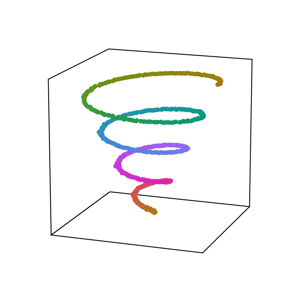
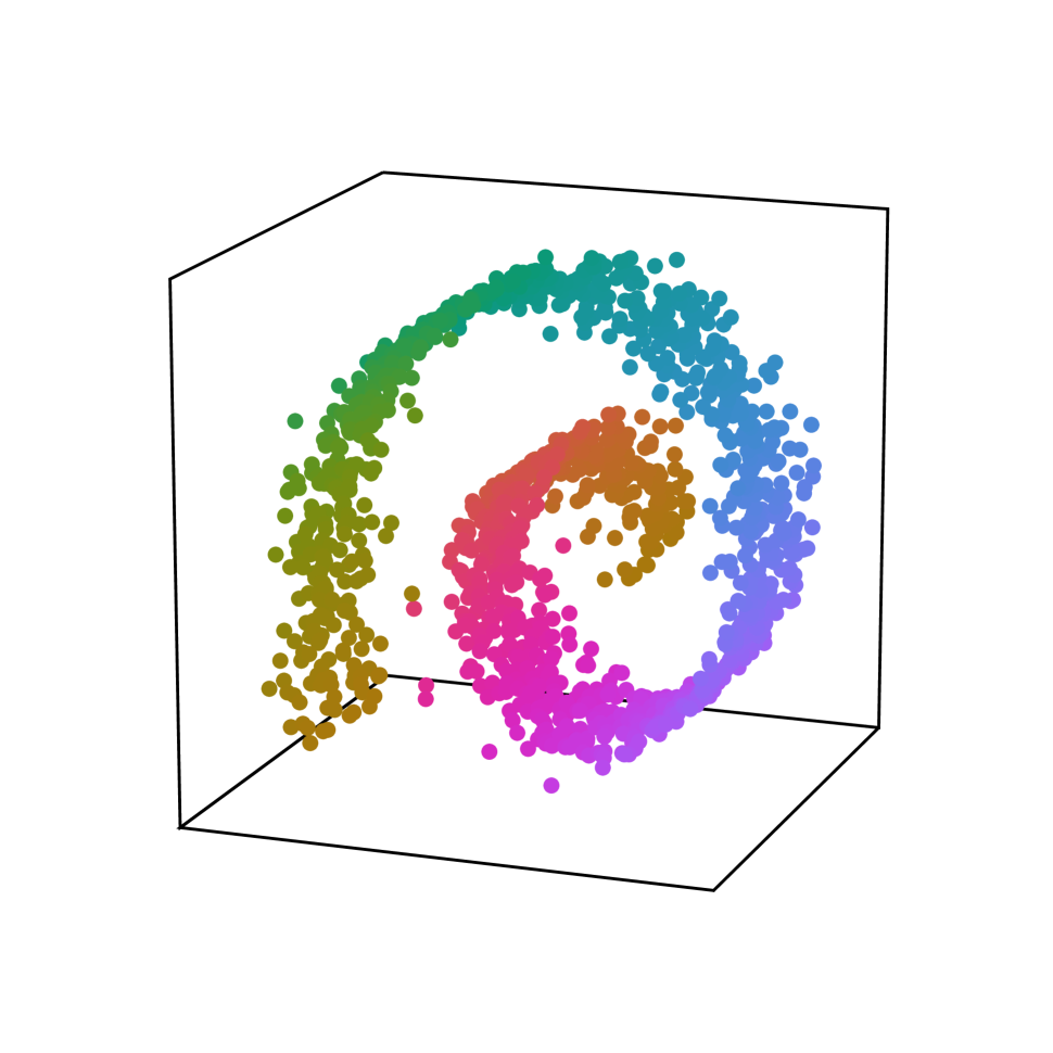
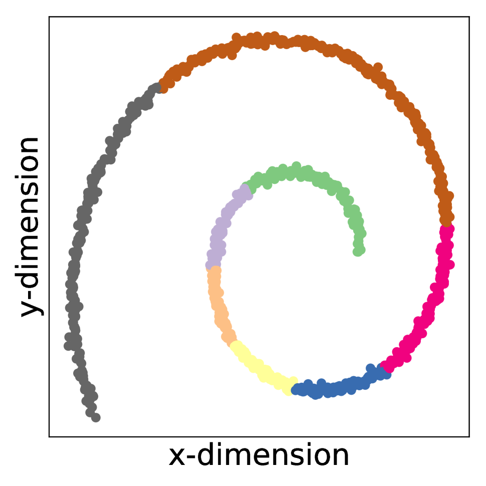
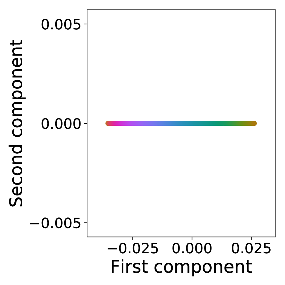
First, we consider two non-linear artificial datasets: the helix and the famous Swiss role dataset. Both datasets are perturbed with a small amount of white Gaussian noise. Figure 2 shows both datasets. The first two components of the diffusion map $\Psi^{t}(x)$ are used to illustrate the non-linear embedding in two dimensional space at time $t=100$. Then, we use the diffusion distance to cluster the data points. Indeed, the diffusion map is able to correctly cluster both non-linear data sets. The width of the Gaussian kernel is set to $\sigma=0.5$.

(a) Noisy helix

(b) Noisy Swiss role

Fig. 2: The top row shows the datasets. The second row shows the clustered data points at diffusion time $t=100$. The third row shows low-dimensional embedding computed using the Nyström-accelerated diffusion map algorithm.

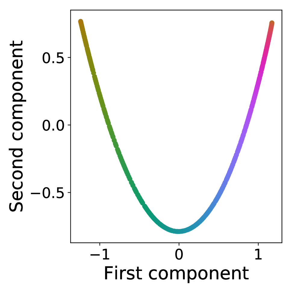
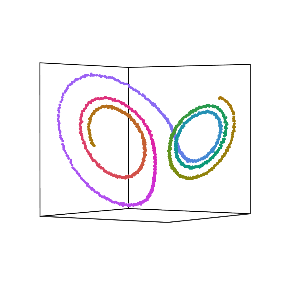
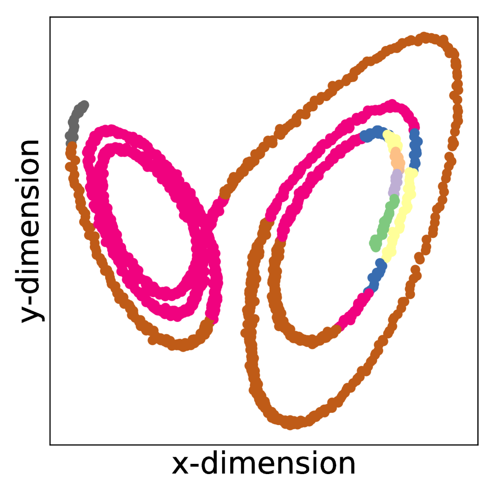
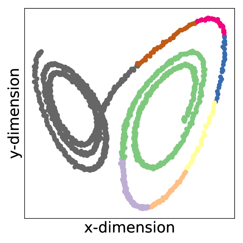
4.2 The Chaotic Lorenz System

Next, we explore the embedding of nonlinear time-series data. Discovering nonlinear transformations that map dynamical systems into a new coordinate system with favorable properties is at the center of modern efforts in data-driven dynamics. One such favorable transformation is obtained by eigenfunctions of the Koopman operator, which provides an infinite-dimensional but linear representation of nonlinear dynamical systems [28, 29, 30]. Diffusion maps have recently been connected to Koopman analysis and are now increasingly being employed to analyze coherent structures and nonlinear embeddings of dynamical systems [31, 32, 33]. Here, we explore the chaotic Lorenz system, which is among the simplest and well-studied chaotic dynamical system [34]:

$$[\dot{x},\,\dot{y},\,\dot{z}]=[\sigma(y-x),\,x(\rho-z)-y,\,xy-\beta z],$$ (18)

with parameters $\sigma\!=\!10,\rho\!=\!28,$ and $\beta\!=\!8/3$. We use the initial conditions $\begin{bmatrix}-8&8&27\end{bmatrix}^{\top}$ and integrate the system from $t\!=\!0$ to $t\!=\!5$ with $\Delta t\approx 0.0001$. Figure 3 shows the results.

(a) Lorenz system

(b) 2-D embedding

(c) Clustered: $t=100$

(d) Clustered: $t=10000$

Fig. 3: The chaotic Lorenz system and its two-dimensional embedding using diffusion maps. Here, a large number of diffusion time steps $t$ is required to obtain stable clusters.

4.3 Computational Performance

Table 1 gives a flavor of the computational performance of the Nyström-accelerated diffusion map algorithm. We achieve substantial computational savings over the deterministic diffusion map algorithm, while attaining small errors. The relative errors between the deterministic $\Psi^{t}(x)$ and randomized diffusion maps $\tilde{\Psi}^{t}(x)$ at $t\!=\!1$ are computed in the Frobenius norm: $||\,|\Psi^{t}(x)|-|\tilde{\Psi}^{t}(x)|\,||_{F}/||\,|\Psi^{t}(x)|\,||_{F}$.

Table 1: Computational performance for both the deterministic and the Nyström accelerated diffusion map algorithm.

Dataset	Number of Observations	Time in s Deterministic	Time in s Nyström	Speedup	Error
Helix	15,000	40	11	3.6	1.8e-13
Swiss role	20,000	72	19	3.7	0.001
Lorenz	30,000	351	115	3.0	0.06

Fig. 4: The Nyström method faithfully captures the dominant eigenvalues of the Gaussian kernel for the Lorenz system.

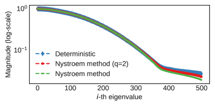
The algorithms are implemented in Python and code is available via GitHub: https://github.com/erichson. The deterministic algorithm uses the fast ARPACK eigensolver provided by SciPy. The Nyström accelerated diffusion map algorithm is computed using random projections with slight oversampling and two additional power iterations $q\!=\!2$. The target-rank (number of components) is set to $d=300$ for the toy data and $d\!=\!500$ for the Lorenz system. Figure 4 shows the approximated eigenvalues for the Lorenz system.

5 Discussion

The computational complexity of diffusion maps scales with the number of observations $n$. Thus, applications such as the analysis of time-series data from dynamical systems pose a computational challenge for diffusion maps. Fortunately, the Nyström method can be used to ease the computational demands. However, diffusion maps are highly sensitive to the approximated range subspace which is provided by the eigenvectors. This means that the Nyström method provides a good approximation only if: (a) the kernel matrix has low-rank structure; (b) the eigenvalue spectrum has a fast decay. The Nyström method shows an excellent performance using random projections with additional power iterations. We achieve a speedup of roughly two to four times when approximating the dominant diffusion map components. Unfortunately, the approximation quality turns out be poor using random column sampling. Future research opens room for a more comprehensive evaluation study. Further, it is of interest to explore kernel functions which are more suitable for dynamical systems, e.g., cone-shaped kernels [35, 31].

References

- [1] C. Burges, “Dimension reduction: A guided tour,” Foundations and Trends in Machine Learning, vol. 2, no. 4, pp. 275–365, 2010.
- [2] L. Van Der Maaten, E. Postma, and J. Van den Herik, “Dimensionality reduction: A comparative review,” Journal of Machine Learning Research, vol. 10, pp. 66–71, 2009.
- [3] S. Lafon, Diffusion maps and geometric harmonics, Ph.D. thesis, Yale University PhD dissertation, 2004.
- [4] R. R. Coifman, S. Lafon, A. B. Lee, M. Maggioni, B. Nadler, F. Warner, and S. W. Zucker, “Geometric diffusions as a tool for harmonic analysis and structure definition of data: Diffusion maps,” Proceedings of the National Academy of Sciences, vol. 102, no. 21, pp. 7426–7431, 2005.
- [5] R. R. Coifman and S. Lafon, “Diffusion maps,” Applied and Computational Harmonic Analysis, vol. 21, no. 1, pp. 5–30, 2006.
- [6] R. R. Coifman, I. G. Kevrekidis, S. Lafon, M. Maggioni, and B. Nadler, “Diffusion maps, reduction coordinates, and low dimensional representation of stochastic systems,” Multiscale Modeling & Simulation, vol. 7, no. 2, pp. 842–864, 2008.
- [7] B. Nadler, S. Lafon, R. R. Coifman, and I. G. Kevrekidis, “Diffusion maps, spectral clustering and reaction coordinates of dynamical systems,” Applied and Computational Harmonic Analysis, vol. 21, no. 1, pp. 113–127, 2006.
- [8] O. Barkan, J. Weill, L. Wolf, and H. Aronowitz, “Fast high dimensional vector multiplication face recognition,” in Proceedings of the IEEE International Conference on Computer Vision, 2013, pp. 1960–1967.
- [9] L. Karacan, E. Erdem, and A. Erdem, “Structure-preserving image smoothing via region covariances,” ACM Trans. Graph., vol. 32, no. 6, pp. 1–11, 2013.
- [10] R. Xu, S. Damelin, and D. C. Wunsch, “Applications of diffusion maps in gene expression data-based cancer diagnosis analysis,” in Engineering in Medicine and Biology Society, 2007. EMBS 2007. 29th Annual International Conference of the IEEE. IEEE, 2007, pp. 4613–4616.
- [11] G. Mishne and I. Cohen, “Multiscale anomaly detection using diffusion maps,” IEEE Journal of Selected Topics in Signal Processing, vol. 7, no. 1, pp. 111–123, 2013.
- [12] N. Halko, P. Martinsson, and J. A. Tropp, “Finding structure with randomness: Probabilistic algorithms for constructing approximate matrix decompositions,” SIAM Review, vol. 53, no. 2, pp. 217–288, 2011.
- [13] M. W. Mahoney, “Randomized algorithms for matrices and data,” Foundations and Trends in Machine Learning, vol. 3, no. 2, pp. 123–224, 2011.
- [14] E. Liberty, “Simple and deterministic matrix sketching,” in Proceedings of the 19th ACM SIGKDD International Conference on Knowledge Discovery and Data Mining. ACM, 2013, pp. 581–588.
- [15] N. B. Erichson, S. Voronin, S. L. Brunton, and J. N. Kutz, “Randomized matrix decompositions using R,” arXiv preprint arXiv:1608.02148, 2016.
- [16] N Benjamin Erichson, Steven L Brunton, and J Nathan Kutz, “Compressed singular value decomposition for image and video processing,” in 2017 IEEE International Conference on Computer Vision Workshop (ICCVW). IEEE, 2017, pp. 1880–1888.
- [17] N. Halko, P. Martinsson, Y. Shkolnisky, and M. Tygert, “An algorithm for the principal component analysis of large data sets,” SIAM Journal on Scientific Computing, vol. 33, no. 5, pp. 2580–2594, 2011.
- [18] V. Rokhlin, A. Szlam, and M. Tygert, “A randomized algorithm for principal component analysis,” SIAM Journal on Matrix Analysis and Applications, vol. 31, no. 3, pp. 1100–1124, 2009.
- [19] N. B. Erichson, A. Mendible, S. Wihlborn, and J. N. Kutz, “Randomized nonnegative matrix factorization,” Pattern Recognition Letters, vol. 104, pp. 1 – 7, 2018.
- [20] N. B. Erichson, S. L. Brunton, and J. N. Kutz, “Randomized dynamic mode decomposition,” arXiv preprint arXiv:1702.02912, 2017.
- [21] N Benjamin Erichson, Krithika Manohar, Steven L Brunton, and J Nathan Kutz, “Randomized cp tensor decomposition,” arXiv preprint arXiv:1703.09074, 2017.
- [22] C. Williams and M. Seeger, “Using the Nyström method to speed up kernel machines,” in Advances in Neural Information Processing Systems 13, pp. 682–688. 2001.
- [23] P. Drineas and M. W. Mahoney, “On the Nyström method for approximating a gram matrix for improved kernel-based learning,” Journal of Machine Learning Research, vol. 6, no. Dec, pp. 2153–2175, 2005.
- [24] F. Chung, Spectral Graph Theory, Number 92. American Mathematical Society, 1997.
- [25] L. Lovász, “Random walks on graphs,” Combinatorics, vol. 2, no. 1-46, pp. 4, 1993.
- [26] E. J. Nyström, “Über die praktische auflösung von integralgleichungen mit anwendungen auf randwertaufgaben,” Acta Mathematica, vol. 54, no. 1, pp. 185–204, 1930.
- [27] S. Kumar, M. Mohri, and A. Talwalkar, “Sampling methods for the nyström method,” Journal of Machine Learning Research, vol. 13, no. Apr, pp. 981–1006, 2012.
- [28] B. O. Koopman, “Hamiltonian systems and transformation in Hilbert space,” Proceedings of the National Academy of Sciences, vol. 17, no. 5, pp. 315–318, 1931.
- [29] I. Mezić, “Spectral properties of dynamical systems, model reduction and decompositions,” Nonlinear Dynamics, vol. 41, no. 1-3, pp. 309–325, 2005.
- [30] S. L. Brunton, B. W. Brunton, J. L. Proctor, and J. N Kutz, “Koopman invariant subspaces and finite linear representations of nonlinear dynamical systems for control,” PLoS ONE, vol. 11, no. 2, pp. e0150171, 2016.
- [31] D. Giannakis, “Dynamics-adapted cone kernels,” SIAM Journal on Applied Dynamical Systems, vol. 14, no. 2, pp. 556–608, 2015.
- [32] T. Berry, D. Giannakis, and J. Harlim, “Nonparametric forecasting of low-dimensional dynamical systems,” Physical Review E, vol. 91, no. 3, pp. 032915, 2015.
- [33] O. Yair, R. Talmon, R. R. Coifman, and I. G. Kevrekidis, “Reconstruction of normal forms by learning informed observation geometries from data,” PNAS, p. 201620045, 2017.
- [34] E. N. Lorenz, “Deterministic nonperiodic flow,” Journal of the Atmospheric Sciences, vol. 20, no. 2, pp. 130–141, 1963.
- [35] Y. Zhao, L. E. Atlas, and R. J. Marks, “The use of cone-shaped kernels for generalized time-frequency representations of nonstationary signals,” IEEE Transactions on Acoustics, Speech, and Signal Processing, vol. 38, no. 7, pp. 1084–1091, 1990.