Sensitivity and Generalization
in Neural Networks: an Empirical Study
Abstract
In practice it is often found that large over-parameterized neural networks generalize better than their smaller counterparts, an observation that appears to conflict with classical notions of function complexity, which typically favor smaller models. In this work, we investigate this tension between complexity and generalization through an extensive empirical exploration of two natural metrics of complexity related to sensitivity to input perturbations. Our experiments survey thousands of models with various fully-connected architectures, optimizers, and other hyper-parameters, as well as four different image classification datasets.
We find that trained neural networks are more robust to input perturbations in the vicinity of the training data manifold, as measured by the norm of the input-output Jacobian of the network, and that it correlates well with generalization. We further establish that factors associated with poor generalization – such as full-batch training or using random labels – correspond to lower robustness, while factors associated with good generalization – such as data augmentation and ReLU non-linearities – give rise to more robust functions. Finally, we demonstrate how the input-output Jacobian norm can be predictive of generalization at the level of individual test points.
1 Introduction
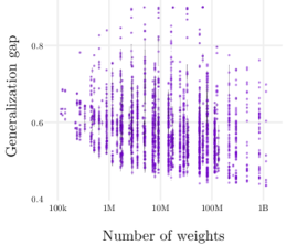
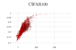
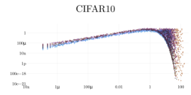
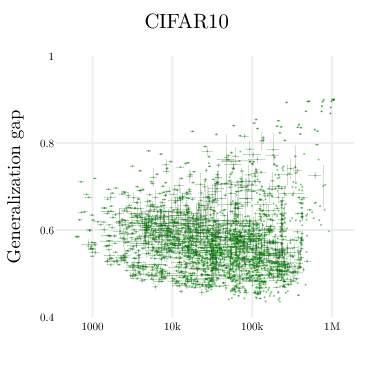
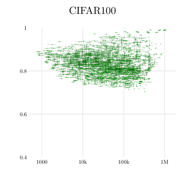
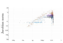
The empirical success of deep learning has thus far eluded interpretation through existing lenses of computational complexity (Blum & Rivest, 1988), numerical optimization (Choromanska et al., 2015; Goodfellow & Vinyals, 2014; Dauphin et al., 2014) and classical statistical learning theory (Zhang et al., 2016): neural networks are highly non-convex models with extreme capacity that train fast and generalize well. In fact, not only do large networks demonstrate good test performance, but larger networks often generalize better, counter to what would be expected from classical measures, such as VC dimension. This phenomenon has been observed in targeted experiments (Neyshabur et al., 2015), historical trends of Deep Learning competitions (Canziani et al., 2016), and in the course of this work (Figure 1).
This observation is at odds with Occam’s razor, the principle of parsimony, as applied to the intuitive notion of function complexity (see §A.2 for extended discussion). One resolution of the apparent contradiction is to examine complexity of functions in conjunction with the input domain. may seem decisively more complex than . But restrained to a narrow input domain of they appear differently: remains a linear function of the input, while resembles a constant . In this work we find that such intuition applies to neural networks, that behave very differently close to the data manifold than away from it (§4.1).
We therefore analyze the complexity of models through their capacity to distinguish different inputs in the neighborhood of datapoints, or, in other words, their sensitivity. We study two simple metrics presented in §3 and find that one of them, the norm of the input-output Jacobian, correlates with generalization in a very wide variety of scenarios.
This work considers sensitivity only in the context of image classification tasks. We interpret the observed correlation with generalization as an expression of a universal prior on (natural) image classification functions that favor robustness (see §A.2 for details). While we expect a similar prior to exist in many other perceptual settings, care should be taken when extrapolating our findings to tasks where such a prior may not be justified (e.g. weather forecasting).

1.1 Paper Outline
We first define sensitivity metrics for fully-connected neural networks in §3. We then relate them to generalization through a sequence of experiments of increasing level of nuance:
-
•
In §4.1 we begin by comparing the sensitivity of trained neural networks on and off the training data manifold, i.e. in the regions of best and typical (over the whole input space) generalization.
-
•
In §4.2 we compare sensitivity of identical trained networks that differ in a single hyper-parameter which is important for generalization.
-
•
Further, §4.3 associates sensitivity and generalization in an unrestricted manner, i.e. comparing networks of a wide variety of hyper-parameters such as width, depth, non-linearity, weight initialization, optimizer, learning rate and batch size.
-
•
Finally, §4.4 explores how predictive sensitivity (as measured by the Jacobian norm) is for individual test points.
1.2 Summary of Contributions
The novelty of this work can be summarized as follows:
-
•
Study of the behavior of trained neural networks on and off the data manifold through sensitivity metrics (§4.1).
- •
§2 puts our work in context of related research studying complexity, generalization, or sensitivity metrics similar to ours.
2 Related Work
2.1 Complexity Metrics
We analyze complexity of fully-connected neural networks for the purpose of model comparison through the following sensitivity measures (see §3 for details):
-
•
estimating the number of linear regions a network splits the input space into;
-
•
measuring the norm of the input-output Jacobian within such regions.
A few prior works have examined measures related to the ones we consider. In particular, Pascanu et al. (2013); Montúfar et al. (2014); Raghu et al. (2016) have investigated the expressive power of fully-connected neural networks built out of piecewise-linear activation functions. Such functions are themselves piecewise-linear over their input domain, so that the number of linear regions into which input space is divided is one measure of how nonlinear the function is. A function with many linear regions has the capacity to build complex, flexible decision boundaries. It was argued in (Pascanu et al., 2013; Montúfar et al., 2014) that an upper bound to the number of linear regions scales exponentially with depth but polynomially in width, and a specific construction was examined. Raghu et al. (2016) derived a tight analytic bound and considered the number of linear regions for generic networks with random weights, as would be appropriate, for instance, at initialization. However, the evolution of this measure after training has not been investigated before. We examine a related measure, the number of hidden unit transitions along one-dimensional trajectories in input space, for trained networks. Further motivation for this measure is discussed in §3.
Another perspective on function complexity can be gained by studying their robustness to perturbations to the input. Indeed, Rasmussen & Ghahramani (2000) demonstrate on a toy problem how complexity as measured by the number of parameters may be of limited utility for model selection, while measuring the output variation allows the invocation of Occam’s razor. In this work we apply related ideas to a large-scale practical context of neural networks with up to a billion free parameters (§4.2, §4.3) and discuss potential ways in which sensitivity permits the application of Occam’s razor to neural networks (§A.2).
Sokolic et al. (2017) provide theoretical support for the relevance of robustness, as measured by the input-output Jacobian, to generalization. They derive bounds for the generalization gap in terms of the Jacobian norm within the framework of algorithmic robustness (Xu & Mannor, 2012). Our results provide empirical support for their conclusions through an extensive number of experiments. In a similar spirit Zahavy et al. (2018) propose a different sensitivity measure in terms of adversarial robustness and relate it to generalization of stochastic algorithms theoretically and experimentally.
Several other recent papers have also focused on deriving tight generalization bounds for neural networks (Bartlett et al., 2017; Dziugaite & Roy, 2017; Neyshabur et al., 2018). We do not propose theoretical bounds in this paper but establish a correlation between our metrics and generalization in a substantially larger experimental setting than undertaken in prior works.
2.2 Regularization
In the context of regularization, increasing robustness to perturbations is a widely-used strategy: data augmentation, noise injection (Jiang et al., 2009), weight decay (Krogh & Hertz, 1992), and max-pooling all indirectly reduce sensitivity of the model to perturbations, while Rifai et al. (2011); Sokolic et al. (2017) explicitly penalize the Frobenius norm of the Jacobian in the training objective.
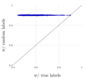
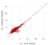
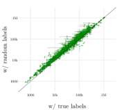
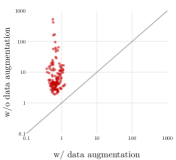
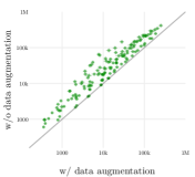
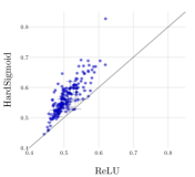
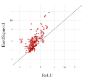
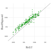
In this work we relate several of the above mentioned regularizing techniques to sensitivity, demonstrating through extensive experiments that improved generalization is consistently coupled with better robustness as measured by a single metric, the input-output Jacobian norm (§4.2). While some of these findings confirm common-sense expectations (random labels increase sensitivity, Figure 4, top row), others challenge our intuition of what makes a neural network robust (ReLU-networks, with unbounded activations, tend to be more robust than saturating HardSigmoid-networks, Figure 4, third row).
2.3 Inductive Bias of SGD
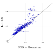
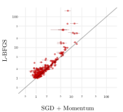
One of our findings demonstrates an inductive bias towards robustness in stochastic mini-batch optimization compared to full-batch training (Figure 4, bottom row). Interpreting this regularizing effect in terms of some measure of sensitivity, such as curvature, is not new (Hochreiter & Schmidhuber, 1997; Keskar et al., 2016), yet we provide a novel perspective by relating it to reduced sensitivity to inputs instead of parameters.
The inductive bias of SGD (“implicit regularization”) has been previously studied in (Neyshabur et al., 2015), where it was shown through rigorous experiments how increasing the width of a single-hidden-layer network improves generalization, and an analogy with matrix factorization was drawn to motivate constraining the norm of the weights instead of their count. Neyshabur et al. (2017) further explored several weight-norm based measures of complexity that do not scale with the size of the model. One of our measures, the Frobenius norm of the Jacobian is of similar nature (since the Jacobian matrix size is determined by the task and not by a particular network architecture). However, this particular metric was not considered, and, to the best of our knowledge, we are the first to evaluate it in a large-scale setting (e.g. our networks are up to layers deep and up to units wide).
2.4 Adversarial Examples
Sensitivity to inputs has attracted a lot of interest in the context of adversarial examples (Szegedy et al., 2013). Several attacks locate points of poor generalization in the directions of high sensitivity of the network (Goodfellow et al., 2014; Papernot et al., 2016; Moosavi-Dezfooli et al., 2016), while certain defences regularize the model by penalizing sensitivity (Gu & Rigazio, 2014) or employing decaying (hence more robust) non-linearities (Kurakin et al., 2016). However, work on adversarial examples relates highly specific perturbations to a similarly specific kind of generalization (i.e. performance on a very small, adversarial subset of the data manifold), while this paper analyzes average-case sensitivity (§3) and typical generalization. Certain measures of adversarial robustness have nevertheless been recently observed to correlate with generalization (Zahavy et al., 2018; Gilmer et al., 2018; Cubuk et al., 2018).
3 Sensitivity Metrics
We propose two simple measures of sensitivity for a fully-connected neural network (without biases) with respect to its input (the output being unnormalized logits of the classes). Assume employs a piecewise-linear activation function, like ReLU. Then itself, as a composition of linear and piecewise-linear functions, is a piecewise-linear map, splitting the input space into disjoint regions, implementing a single affine mapping on each. Then we can measure two aspects of sensitivity by answering
-
1.
How does the output of the network change as the input is perturbed within the linear region?
-
2.
How likely is the linear region to change in response to change in the input?
We quantify these qualities as follows:
-
1.
For a local sensitivity measure we adopt the Frobenius norm of the class probabilities Jacobian (with ), where with being the softmax function111The norm of the Jacobian with respect to logits experimentally turned out less predictive of test performance (not shown). See §A.3 for discussion of why the softmax Jacobian is related to generalization.. Given points of interest , we estimate the sensitivity of the function in those regions with the average Jacobian norm:
that we will further refer to as simply “Jacobian norm”. Note that this does not require the labels for .
Interpretation. The Frobenius norm estimates the average-case sensitivity of around . Indeed, consider an infinitesimal Gaussian perturbation : the expected magnitude of the output change is then
-
2.
To detect a change in linear region (further called a “transition”), we need to be able to identify it. We do this analogously to Raghu et al. (2016). For a network with piecewise-linear activations, we can, given an input , assign a code to each neuron in the network , that identifies the linear region of the pre-activation of that neuron. E.g. each ReLU unit will have or assigned to it if the pre-activation value is less or greater than respectively. Similarly, a ReLU6 unit (see definition in §A.4) will have a code of , , or assigned, since it has linear regions222For a non-piecewise-linear activation like Tanh, we consider as the boundary of two regions and find this metric qualitatively similar to counting transitions of a piecewise-linear non-linearity.. Then, a concatenation of codes of all neurons in the network (denoted by ) uniquely identifies the linear region of the input (see §A.1.1 for discussion of edge cases).
Given this encoding scheme, we can detect a transition by detecting a change in the code. We then sample equidistant points on a closed one-dimensional trajectory (generated from a data point and lying close to the data manifold; see below for details) and count transitions along it to quantify the number of linear regions:
(1) where the norm of the directional derivative amounts to a Dirac delta function at each transition (see §A.1.2 for further details).
By sampling multiple such trajectories around different points, we estimate the sensitivity metric:
that we will further refer to as simply “transitions” or “number of transitions.”
To assure the sampling trajectory is close to the data manifold (since this is the region of interest), we construct it through horizontal translations of the image in pixel space (Figure App.9, right). We similarly augment our training data with horizontal and vertical translations in the corresponding experiments (Figure 4, second row).
As earlier, this metric does not require knowing the label of .
Interpretation. We can draw a qualitative parallel between the number of transitions and curvature of the function. One measure of curvature of a function is the total norm of the directional derivative of its first derivative along a path:
A piecewise-linear function has a constant first derivative everywhere except for the transition boundaries. Therefore, for a sufficiently large , curvature can be expressed as
where are equidistant samples on . This sum is similar to as defined in Equation 1, but quantifies the amount of change in between two linear regions in a non-binary way. However, estimating it on a densely sampled trajectory is a computationally-intensive task, which is one reason we instead count transitions.
As such, on a qualitative level, the two metrics (Jacobian norm and number of transitions) track the first and second order terms of the Taylor expansion of the function.
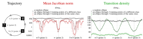
Above we have defined two sensitivity metrics to describe the learned function around the data, on average. In §4.1 we analyze these measures on and off the data manifold by simply measuring them along circular trajectories in input space that intersect the data manifold at certain points, but generally lie away from it (Figure 2, left).
4 Experimental Results
In the following subsections (§4.2, §4.3) each study analyzes performance of a large number (usually thousands) of fully-connected neural networks having different hyper-parameters and optimization procedures. Except where specified, we include only models which achieve training accuracy. This allows us to study generalization disentangled from properties like expressivity and trainability, which are outside the scope of this work.
In order to efficiently evaluate the compute-intensive metrics (§3) in a very wide range of hyper-parameters settings (see e.g. §A.5.5) we only consider fully-connected networks. Extending the investigation to more complex architectures is left for future work.
4.1 Sensitivity On and Off the Training Data Manifold
We analyze the behavior of a trained neural network near and away from training data. We do this by comparing sensitivity of the function along 3 types of trajectories:
-
1.
A random ellipse. This trajectory is extremely unlikely to pass anywhere near the real data, and indicates how the function behaves in random locations of the input space that it never encountered during training.
-
2.
An ellipse passing through three training points of different class (Figure 2, left). This trajectory does pass through the three data points, but in between it traverses images that are linear combinations of different-class images, and are expected to lie outside of the natural image space. Sensitivity of the function along this trajectory allows comparison of its behavior on and off the data manifold, as it approaches and moves away from the three anchor points.
-
3.
An ellipse through three training points of the same class. This trajectory is similar to the previous one, but, given the dataset used in the experiment (MNIST), is expected to traverse overall closer to the data manifold, since linear combinations of the same digit are more likely to resemble a realistic image. Comparing transition density along this trajectory to the one through points of different classes allows further assessment of how sensitivity changes in response to approaching the data manifold.
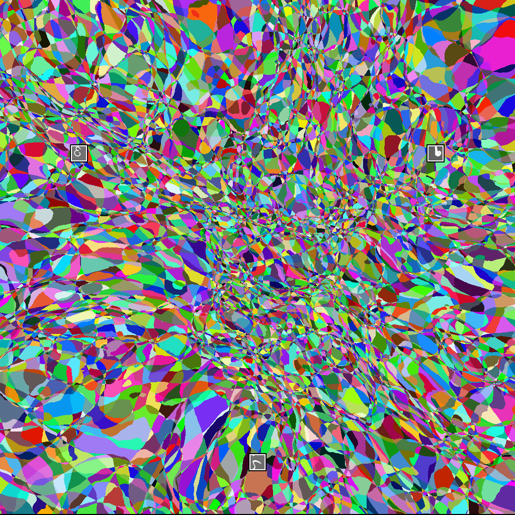
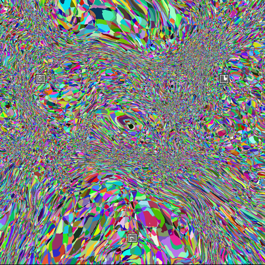
We find that, according to both the Jacobian norm and transitions metrics, functions exhibit much more robust behavior around the training data (Figure 2, center and right). We further visualize this effect in 2D in Figure 3, where we plot the transition boundaries of the last (pre-logit) layer of a neural network before and after training. After training we observe that training points lie in regions of low transition density.
The observed contrast between the neural network behavior near and away from data further strengthens the empirical connection we draw between sensitivity and generalization in §4.2, §4.3 and §4.4; it also confirms that, as mentioned in §1, if a certain quality of a function is to be used for model comparison, input domain should always be accounted for.
Before Training After Training
4.2 Sensitivity and Generalization Factors
In §4.1 we established that neural networks implement more robust functions in the vicinity of the training data manifold than away from it.
We now consider the more practical context of model selection. Given two perfectly trained neural networks, does the model with better generalization implement a less sensitive function?
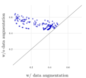
We study approaches in the machine learning community that are commonly believed to influence generalization (Figure 4, top to bottom):
-
•
random labels;
-
•
data augmentation;
-
•
ReLUs;
-
•
full-batch training.
We find that in each case, the change in generalization is coupled with the respective change in sensitivity (i.e. lower sensitivity corresponds to smaller generalization gap) as measured by the Jacobian norm (and almost always for the transitions metric).
| Generalization Gap | Jacobian norm | Transitions |
|---|---|---|
 |
 |
 |
 |
 |
 |
 |
 |
 |
 |
 |
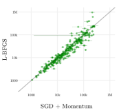 |
4.2.1 How to Read Plots
In Figure 4, for many possible hyper-parameter configurations, we train two models that share all parameters and optimization procedure, but differ in a single binary setting (i.e. trained on true or random labels; with or without data augmentation; etc). Out of all such network pairs, we select only those where each network reached 100% training accuracy on the whole training set (apart from the data augmentation study). The two generalization or sensitivity values are then used as the and coordinates of a point corresponding to this pair of networks (with the plot axes labels denoting the respective value of the binary parameter considered). The position of the point with respect to the diagonal visually demonstrates which configuration has smaller generalization gap / lower sensitivity.
4.3 Sensitivity and Generalization Gap
We now perform a large-scale experiment to establish direct relationships between sensitivity and generalization in a realistic setting. In contrast to §4.1, where we selected locations in the input space, and §4.2, where we varied a single binary parameter impacting generalization, we now sweep simultaneously over many different architectural and optimization choices (§A.5.5).
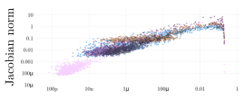
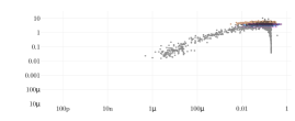
Our main result is presented in Figure 5, indicating a strong relationship between the Jacobian norm and generalization. In contrast, Figure App.8 demonstrates that the number of transitions is not alone sufficient to compare networks of different sizes, as the number of neurons in the networks has a strong influence on transition count.

Jacobian norm
4.4 Sensitivity and Per-Point Generalization
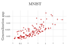
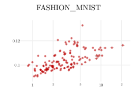
In §4.3 we established a correlation between sensitivity (as measured by the Jacobian norm) and generalization averaged over a large test set ( points). We now investigate whether the Jacobian norm can be predictive of generalization at individual points.
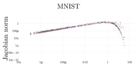
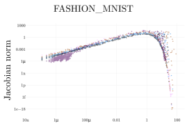
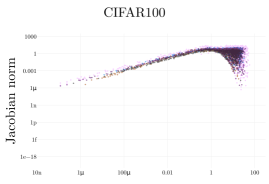
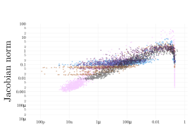
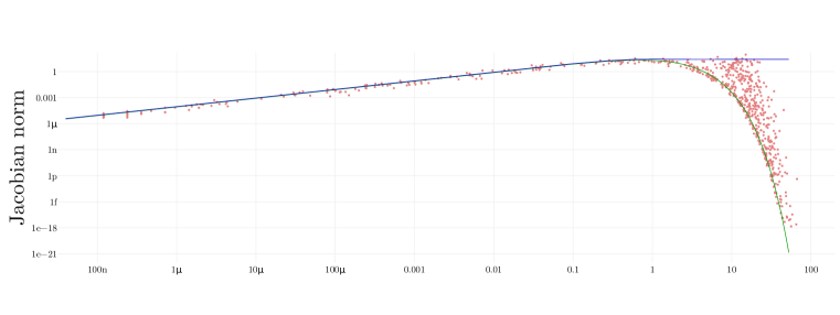
As demonstrated in Figure 6 (top), Jacobian norm at a point is predictive of the cross-entropy loss, but the relationship is not a linear one, and not even bijective (see §A.3 for analytic expressions explaining it). In particular, certain misclassified points (right sides of the plots) have a Jacobian norm many orders of magnitude smaller than that of the correctly classified points (left sides). However, we do remark a consistent tendency for points having the highest values of the Jacobian norm to be mostly misclassified. A similar yet noisier trend is observed in networks trained using -loss as depicted in Figure 6 (bottom). These observations make the Jacobian norm a promising quantity to consider in the contexts of active learning and confidence estimation in future research.
Cross-entropy loss
-loss
5 Conclusion
We have investigated sensitivity of trained neural networks through the input-output Jacobian norm and linear regions counting in the context of image classification tasks. We have presented extensive experimental evidence indicating that the local geometry of the trained function as captured by the input-output Jacobian can be predictive of generalization in many different contexts, and that it varies drastically depending on how close to the training data manifold the function is evaluated. We further established a connection between the cross-entropy loss and the Jacobian norm, indicating that it can remain informative of generalization even at the level of individual test points. Interesting directions for future work include extending our investigation to more complex architectures and other machine learning tasks.
References
- Abadi et al. (2016) Martín Abadi, Ashish Agarwal, Paul Barham, Eugene Brevdo, Zhifeng Chen, Craig Citro, Greg S Corrado, Andy Davis, Jeffrey Dean, Matthieu Devin, et al. Tensorflow: Large-scale machine learning on heterogeneous distributed systems. arXiv preprint arXiv:1603.04467, 2016.
- Bartlett et al. (2017) Peter L Bartlett, Dylan J Foster, and Matus J Telgarsky. Spectrally-normalized margin bounds for neural networks. In Advances in Neural Information Processing Systems, pp. 6241–6250, 2017.
- Blum & Rivest (1988) Avrim Blum and Ronald L. Rivest. Training a 3-node neural network is np-complete. In Machine Learning: From Theory to Applications, 1988.
- Canziani et al. (2016) Alfredo Canziani, Adam Paszke, and Eugenio Culurciello. An analysis of deep neural network models for practical applications. CoRR, abs/1605.07678, 2016.
- Choromanska et al. (2015) Anna Choromanska, Mikael Henaff, Michael Mathieu, Gérard Ben Arous, and Yann LeCun. The loss surfaces of multilayer networks. In Artificial Intelligence and Statistics, pp. 192–204, 2015.
- Cubuk et al. (2018) Ekin Dogus Cubuk, Barret Zoph, Samuel Stern Schoenholz, and Quoc V. Le. Intriguing properties of adversarial examples. In International Conference on Learning Representations - Workshop Track, 2018. URL https://arxiv.org/abs/1801.02774.
- Dauphin et al. (2014) Yann Dauphin, Razvan Pascanu, Çaglar Gülçehre, Kyunghyun Cho, Surya Ganguli, and Yoshua Bengio. Identifying and attacking the saddle point problem in high-dimensional non-convex optimization. In NIPS, 2014.
- Dziugaite & Roy (2017) Gintare Karolina Dziugaite and Daniel M Roy. Computing nonvacuous generalization bounds for deep (stochastic) neural networks with many more parameters than training data. arXiv preprint arXiv:1703.11008, 2017.
- Gilmer et al. (2018) Justin Gilmer, Luke Metz, Fartash Faghri, Sam Schoenholz, Maithra Raghu, Martin Wattenberg, and Ian Goodfellow. Adversarial spheres. In International Conference on Learning Representations - Workshop Track, 2018. URL https://arxiv.org/abs/1801.02774.
- Golovin et al. (2017) Daniel Golovin, Benjamin Solnik, Subhodeep Moitra, Greg Kochanski, John Karro, and D Sculley. Google vizier: A service for black-box optimization. In Proceedings of the 23rd ACM SIGKDD International Conference on Knowledge Discovery and Data Mining, pp. 1487–1495. ACM, 2017.
- Goodfellow & Vinyals (2014) Ian J. Goodfellow and Oriol Vinyals. Qualitatively characterizing neural network optimization problems. CoRR, abs/1412.6544, 2014.
- Goodfellow et al. (2014) Ian J Goodfellow, Jonathon Shlens, and Christian Szegedy. Explaining and harnessing adversarial examples. arXiv preprint arXiv:1412.6572, 2014.
- Gu & Rigazio (2014) Shixiang Gu and Luca Rigazio. Towards deep neural network architectures robust to adversarial examples. arXiv preprint arXiv:1412.5068, 2014.
- Gulcehre et al. (2016) Caglar Gulcehre, Marcin Moczulski, Misha Denil, and Yoshua Bengio. Noisy activation functions. In International Conference on Machine Learning, pp. 3059–3068, 2016.
- Hinton et al. (2012) Geoffrey Hinton, Nitish Srivastava, and Kevin Swersky. Neural networks for machine learning-lecture 6a-overview of mini-batch gradient descent, 2012.
- Hochreiter & Schmidhuber (1997) Sepp Hochreiter and Jürgen Schmidhuber. Flat minima. Neural Computation, 9(1):1–42, 1997.
- Jefferys & Berger (1992) William H Jefferys and James O Berger. Ockham’s razor and bayesian analysis. American Scientist, 80(1):64–72, 1992.
- Jiang et al. (2009) Yulei Jiang, Richard M Zur, Lorenzo L Pesce, and Karen Drukker. A study of the effect of noise injection on the training of artificial neural networks. In Neural Networks, 2009. IJCNN 2009. International Joint Conference on, pp. 1428–1432. IEEE, 2009.
- Keskar et al. (2016) Nitish Shirish Keskar, Dheevatsa Mudigere, Jorge Nocedal, Mikhail Smelyanskiy, and Ping Tak Peter Tang. On large-batch training for deep learning: Generalization gap and sharp minima. arXiv preprint arXiv:1609.04836, 2016.
- Kingma & Ba (2014) Diederik Kingma and Jimmy Ba. Adam: A method for stochastic optimization. arXiv preprint arXiv:1412.6980, 2014.
- Krizhevsky (2010) Alex Krizhevsky. Convolutional deep belief networks on cifar-10. 2010.
- Krogh & Hertz (1992) Anders Krogh and John A Hertz. A simple weight decay can improve generalization. In Advances in neural information processing systems, pp. 950–957, 1992.
- Kurakin et al. (2016) Alexey Kurakin, Ian Goodfellow, and Samy Bengio. Adversarial machine learning at scale. arXiv preprint arXiv:1611.01236, 2016.
- Lee et al. (2018) Jaehoon Lee, Yasaman Bahri, Roman Novak, Sam Schoenholz, Jeffrey Pennington, and Jascha Sohl-dickstein. Deep neural networks as gaussian processes. In International Conference on Learning Representations, 2018. URL https://arxiv.org/abs/1711.00165.
- MacKay (1991) David JC MacKay. Bayesian interpolation. 1991.
- MacKay (1992) David JC MacKay. A practical bayesian framework for backpropagation networks. Neural computation, 4(3):448–472, 1992.
- Montúfar et al. (2014) G. Montúfar, R. Pascanu, K. Cho, and Y. Bengio. On the Number of Linear Regions of Deep Neural Networks. Neural Information Processing Systems, February 2014.
- Moosavi-Dezfooli et al. (2016) Seyed-Mohsen Moosavi-Dezfooli, Alhussein Fawzi, Omar Fawzi, and Pascal Frossard. Universal adversarial perturbations. arXiv preprint arXiv:1610.08401, 2016.
- Murray & Ghahramani (2005) Iain Murray and Zoubin Ghahramani. A note on the evidence and bayesian occam’s razor, 2005.
- Nair & Hinton (2010) Vinod Nair and Geoffrey E Hinton. Rectified linear units improve restricted boltzmann machines. In Proceedings of the 27th international conference on machine learning (ICML-10), pp. 807–814, 2010.
- Neal (1994) Radford M. Neal. Priors for infinite networks (tech. rep. no. crg-tr-94-1). University of Toronto, 1994.
- Neyshabur et al. (2015) Behnam Neyshabur, Ryota Tomioka, and Nathan Srebro. In search of the real inductive bias: On the role of implicit regularization in deep learning. Proceeding of the international Conference on Learning Representations workshop track, abs/1412.6614, 2015.
- Neyshabur et al. (2017) Behnam Neyshabur, Srinadh Bhojanapalli, David McAllester, and Nathan Srebro. Exploring generalization in deep learning. CoRR, abs/1706.08947, 2017.
- Neyshabur et al. (2018) Behnam Neyshabur, Srinadh Bhojanapalli, and Nathan Srebro. A PAC-bayesian approach to spectrally-normalized margin bounds for neural networks. In International Conference on Learning Representations, 2018. URL https://openreview.net/forum?id=Skz_WfbCZ.
- Papernot et al. (2016) Nicolas Papernot, Patrick McDaniel, Somesh Jha, Matt Fredrikson, Z Berkay Celik, and Ananthram Swami. The limitations of deep learning in adversarial settings. In Security and Privacy (EuroS&P), 2016 IEEE European Symposium on, pp. 372–387. IEEE, 2016.
- Pascanu et al. (2013) R. Pascanu, G. Montufar, and Y. Bengio. On the number of response regions of deep feed forward networks with piece-wise linear activations. International Conference on Learning Representations, December 2013.
- Poole et al. (2016) B. Poole, S. Lahiri, M. Raghu, J. Sohl-Dickstein, and S. Ganguli. Exponential expressivity in deep neural networks through transient chaos. Neural Information Processing Systems, June 2016.
- Raghu et al. (2016) M. Raghu, B. Poole, J. Kleinberg, S. Ganguli, and J. Sohl-Dickstein. On the Expressive Power of Deep Neural Networks. International Conference on Machine Learning, June 2016.
- Rasmussen & Ghahramani (2000) Carl E. Rasmussen and Zoubin Ghahramani. Occam’s razor. In NIPS, 2000.
- Rifai et al. (2011) Salah Rifai, Pascal Vincent, Xavier Muller, Xavier Glorot, and Yoshua Bengio. Contractive auto-encoders: Explicit invariance during feature extraction. In Proceedings of the 28th international conference on machine learning (ICML-11), pp. 833–840, 2011.
- Rumelhart et al. (1988) David E Rumelhart, Geoffrey E Hinton, Ronald J Williams, et al. Learning representations by back-propagating errors. Cognitive modeling, 5(3):1, 1988.
- Sokolic et al. (2017) Jure Sokolic, Raja Giryes, Guillermo Sapiro, and Miguel RD Rodrigues. Robust large margin deep neural networks. IEEE Transactions on Signal Processing, 2017.
- Solak et al. (2003) Ercan Solak, Roderick Murray-Smith, William E Leithead, Douglas J Leith, and Carl E Rasmussen. Derivative observations in gaussian process models of dynamic systems. In Advances in neural information processing systems, pp. 1057–1064, 2003.
- Szegedy et al. (2013) Christian Szegedy, Wojciech Zaremba, Ilya Sutskever, Joan Bruna, Dumitru Erhan, Ian Goodfellow, and Rob Fergus. Intriguing properties of neural networks. arXiv preprint arXiv:1312.6199, 2013.
- Telgarsky (2015) Matus Telgarsky. Representation benefits of deep feedforward networks. CoRR, abs/1509.08101, 2015.
- Xiao et al. (2017) Han Xiao, Kashif Rasul, and Roland Vollgraf. Fashion-mnist: a novel image dataset for benchmarking machine learning algorithms, 2017.
- Xu & Mannor (2012) Huan Xu and Shie Mannor. Robustness and generalization. Machine learning, 86(3):391–423, 2012.
- Zahavy et al. (2018) Tom Zahavy, Bingyi Kang, Alex Sivak, Jiashi Feng, Huan Xu, and Shie Mannor. Ensemble robustness and generalization of stochastic deep learning algorithms. In International Conference on Learning Representations - Workshop Track, 2018. URL https://openreview.net/forum?id=r1YUtYx0-.
- Zhang et al. (2016) C. Zhang, S. Bengio, M. Hardt, B. Recht, and O. Vinyals. Understanding deep learning requires rethinking generalization. International Conference on Learning Representations, November 2016.
Appendix A Appendix
Transitions
Cross-entropy loss
-loss
A.1 Transition Metric Details
A.1.1 Linear Region Encoding
The way of encoding a linear region of a point described in §3 (2) guarantees that different regions obtain different codes, but different codes might be assigned to the same region if all the neurons in any layer of the network are saturated (or if weights leading from the transitioning unit to active units are exactly zero, or exactly cancel). However, the probability of such an arrangement drops exponentially with width and hence is ignored in this work.
A.1.2 Transition Counting
The equality between the discrete and continuous versions of in Equation 1 becomes exact with a high-enough sampling density such that there are no narrow linear regions missed in between consecutive points (precisely, the encoding has to only change at most once on the line between two consecutive points and ).
For computational efficiency we also assume that no two neurons transitions simultaneously, which is extremely unlikely in the context of random initialization and stochastic optimization.
A.2 Do neural networks defy Occam’s razor?
Here we briefly discuss the motivation of this work in the context of Occam’s razor.
Occam’s razor is a heuristic for model comparison based on their complexity. Given a dataset , Occam’s razor gives preference to simpler models . In the Bayesian interpretation of the heuristic (Jefferys & Berger, 1992) simplicity is defined as evidence and is often computed using the Laplace approximation. Under further assumptions (MacKay, 1991), this evidence can be shown to be inversely proportional to the number of parameters in the model. Therefore, given a uniform prior on two competing hypothesis classes, the class posterior is higher for a model with fewer parameters.
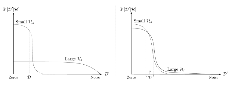
An alternative, qualitative justification of the heuristic is through considering the evidence as a normalized probability distribution over the whole dataset space:
and remarking that models with more parameters have to spread the probability mass more evenly across all the datasets by virtue of being able to fit more of them (Figure App.10, left). This similarly suggests (under a uniform prior on competing hypothesis classes) preferring models with fewer parameters, assuming that evidence is unimodal and peaks close to the dataset of interest.
Occam’s razor for neural networks. As seen in Figure 1, the above reasoning does not apply to neural networks: the best achieved generalization is obtained by a model that has around times as many parameters as the simplest model capable of fitting the dataset (within the evaluated search space).
On one hand, Murray & Ghahramani (2005); Telgarsky (2015) demonstrate on concrete examples that a high number of free parameters in the model doesn’t necessarily entail high complexity. On the other hand, a large body of work on the expressivity of neural networks (Pascanu et al., 2013; Montúfar et al., 2014; Raghu et al., 2016; Poole et al., 2016) shows that their ability to compute complex functions increases rapidly with size, while Zhang et al. (2016) validates that they also easily fit complex (even random) functions with stochastic optimization. Classical metrics like VC dimension or Rademacher complexity increase with size of the network as well. This indicates that weights of a neural network may actually correspond to its usable capacity, and hence “smear” the evidence along a very large space of datasets , making the dataset of interest less likely.
Potential issues. We conjecture the Laplace approximation of the evidence and the simplified estimation of the “Occam’s factor” in terms of the accessible volume of the parameter space might not hold for neural networks in the context of stochastic optimization, and, in particular, do not account for the combinatorial growth of the accessible volume of parameter space as width increases (MacKay, 1992). Similarly, when comparing evidence as probability distributions over datasets, the difference between two neural networks may not be as drastic as in Figure App.10 (left), but more nuanced as depicted in Figure App.10 (right), with the evidence ratio being highly dependent on the particular dataset.
Expectation Reality?
We interpret our work as defining hypothesis classes based on sensitivity of the hypothesis (which yielded promising results in (Rasmussen & Ghahramani, 2000) on a toy task) and observing a strongly non-uniform prior on these classes that enables model comparison. Indeed, at least in the context of natural images classification, putting a prior on the number of parameters or Kolmogorov complexity of the hypothesis is extremely difficult. However, a statement that the true classification function is robust to small perturbations in the input is much easier to justify. As such, a prior in favor of robustness over sensitivity might fare better than a prior on specific network hyper-parameters.
Above is one way to interpret the correlation between sensitivity and generalization that we observe in this work. It does not explain why large networks tend to converge to less sensitive functions. We conjecture large networks to have access to a larger space of robust solutions due to solving a highly-underdetermined system when fitting a dataset, while small models converge to more extreme weight values due to being overconstrained by the data. However, further investigation is needed to confirm this hypothesis.
A.3 Bounding the Jacobian Norm
Here we analyze the relationship between the Jacobian norm and the cross-entropy loss at individual test points as studied in §4.4.
Target class Jacobian. We begin by relating the derivative of the target class probability to per-point cross-entropy loss (where is the correct integer class).
We will denote by and drop the argument to de-clutter notation (i.e. write instead of ). Then the Jacobian can be expressed as
where is the Hadamard element-wise product. Then indexing both sides of the equation at the correct class yields
where is a vector of zeros everywhere except for . Taking the norm of both sides results in
| (2) | ||||
| (3) | ||||
| (4) |
We now assume that magnitudes of the individual logit derivatives vary little in between logits and over the input space333In the limit of infinite width, and fully Bayesian training, deep network logits are distributed exactly according to a Gaussian process (Neal, 1994; Lee et al., 2018). Similarly, each entry in the logit Jacobian also corresponds to an independent draw from a Gaussian process (Solak et al., 2003). It is therefore plausible that the Jacobian norm, consisting of a sum over the square of independent Gaussian samples in the correct limits, will tend towards a constant.:
which simplifies Equation 4 to
where . Since lies on the -simplex , under these assumptions we can bound:
and finally
or, in terms of the cross-entropy loss :
| (5) |
We validate these approximate bounds in Figure App.11 (top).
Full Jacobian. Equation 5 establishes a close relationship between and loss , but of course, at test time we do not know the target class . This allows us to only bound the full Jacobian norm from below:
| (6) |
For the upper bound, we assume the maximum-entropy case of : , for . The Jacobian norm is
where the first summand becomes:
and each of the others
Adding of such summands to results in
| (7) |
compared against the lower bound (Equation 6) and experimental data in Figure App.11.
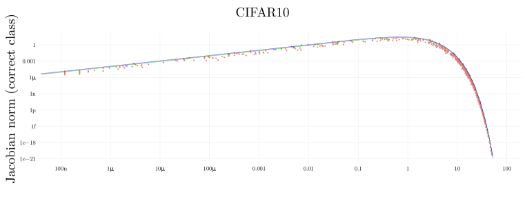
Cross-entropy loss
A.4 Non-linearities Definitions
A.5 Experimental Setup
All experiments were implemented in Tensorflow (Abadi et al., 2016) and executed with the help of Vizier (Golovin et al., 2017). All networks were trained with cross-entropy loss. All networks were trained without biases. All computations were done with 32-bit precision. Learning rate decayed by a factor of every epochs.
Unless specified otherwise, initial weights were drawn from a normal distribution with zero mean and variance for ReLU, ReLU6 and HardSigmoid; for Tanh and HardTanh, where is the number of inputs to the current layer.
All inputs were normalized to have zero mean and unit variance, or, in other terms, lie on the -dimensional sphere of radius , where is the dimensionality of the input.
All reported values, when applicable, were evaluated on the whole training and test sets of sizes and respectively. E.g. “generalization gap” is defined as the difference between train and test accuracies evaluated on the whole train and test sets.
When applicable, all trajectories/surfaces in input space were sampled with points.
A.5.1 Plots and Error Bars
All figures except for 6 and App.11 are plotted with (pale) error bars (when applicable). The reported quantity was usually evaluated times with random seeds from to 444If a particular random seed did not finish, it was not taken into account; we believe this nuance did not influence the conclusions of this paper., unless specified otherwise. E.g. if a network is said to be 100%-accurate on the training set, it means that each of the randomly-initialized networks is 100%-accurate after training.
The error bar is centered at the mean value of the quantity and spans the standard error of the mean in each direction. If the bar appears to not be visible, it may be smaller than the mean value marker.
Weight initialization, training set shuffling, data augmentation, picking anchor points of data-fitted trajectories, selecting axes of a zero-centered elliptic trajectory depend on the random seed.
A.5.2 Sensitivity along a Trajectory
Relevant figure 2.
A 20-layer ReLU-network of width 200 was trained on MNIST 128 times, with plots displaying the averaged values.
A random zero-centered ellipse was obtained by generating two axis vectors with normally-distributed entries of zero mean and unit variance (as such making points on the trajectory have an expected norm equal to that of training data) and sampling points on the ellipse with given axes.
A random data-fitted ellipse was generated by projecting three arbitrary input points onto a plane where they fall into vertices of an equilateral triangle, and then projecting their circumcircle back into the input space.
A.5.3 Linear Region Boundaries
Relevant figure 3.
A 15-layer ReLU6-network of width 300 was trained on MNIST for steps using SGD with momentum (Rumelhart et al., 1988); images were randomly translated with wrapping by up to 4 pixels in each direction, horizontally and vertically, as well as randomly flipped along each axis, and randomly rotated by degrees clockwise and counter-clockwise.
The sampling grid in input space was obtain by projecting three arbitrary input points into a plane as described in §A.5.2 such that the resulting triangle was centered at and it’s vertices were at a distance form the origin. Then, a sampling grid of points in the square was projected back into the input space.
A.5.4 Small Experiment
All networks were trained for steps of batch size of using SGD with momentum. Learning rate was set to and momentum term coefficient to .
Data augmentation consisted of random translation of the input by up to 4 pixels in each direction with wrapping, horizontally and vertically. The input was also flipped horizontally with probability . When applying data augmentation (second row of Figure 4), the network is unlikely to encounter the canonical training data, hence few configurations achieved training accuracy. However, we verified that all networks trained with data augmentation reached a higher test accuracy than their analogues without, ensuring that the generalization gap shrinks not simply because of lower training accuracy.
For each dataset, networks of width , depth and activation function were evaluated on random seeds from to .
A.5.5 Large Experiment
networks were trained for steps with random hyper-parameters; if training did not complete, a checkpoint at step was used instead, if available. When using L-BFGS, the maximum number of iterations was set to . The space of available hyper-parameters included555Due to time and compute limitations, this experiment was set up such that configurations of small size were more likely to get evaluated (e.g. only a few networks of width were trained, and all of them had depth ). However, based on our experience with smaller experiments (where each configuration got evaluated), we believe this did not bias the findings of this paper, while allowing them to be validated across a very wide range of scenarios.:
-
1.
CIFAR10 and CIFAR100 datasets cropped to a center region;
-
2.
all 5 non-linearities from §A.4;
- 3.
-
4.
learning rates from , when applicable. Secondary coefficients were fixed at default values of Tensorflow implementations of respective optimizers;
-
5.
batch sizes of (unless using L-BFGS with the full batch of );
-
6.
standard deviations of initial weights from multiplied by the default value described in §A.5;
-
7.
widths from ;
-
8.
depths from ;
-
9.
true and random training labels;
-
10.
random seeds from to .
A.5.6 Per-point Generalization
Networks were with either cross-entropy or -loss trained for steps on whole datasets (CIFAR100, CIFAR10, Fashion-MNIST and MNIST) and evaluated on random subsets of test images.
Hyper-parameters were: non-linearity (all functions from §A.4), width (, , , , ), depth (, , , , ), learning rate (, , ), optimizer (SGD, Momentum, ADAM, RMSProp). Only one random seed (1) was used. For each dataset a random subset of 5 configurations among all the -accurate (on training) networks was plotted (apart from the case of CIFAR100, where networks of training accuracy of at least were selected).
A.5.7 Cross-entropy and Sensitivity Analysis
Relevant figure App.11.
Networks were trained for on the whole CIFAR10 training set and evaluated networks on a random test subset of size . The hyper-parameters consisted of non-linearity (all functions from §A.4), width (, or ) and depth (, , , ). Only one random seed () was considered. A single random 100%-accurate (on training data) network was drawn to compare experimental measurements with analytic bounds on the Jacobian norm.