Electronic entropy in Green’s-function calculations at finite temperatures

Abstract

We revise critically existing approaches to evaluation of thermodynamic potentials within the Green’s function calculations at finite electronic temperatures. We focus on the entropy and show that usual technical problems related to the multivalued nature of the complex logarithm can be overcome. This results in a simple expression for the electronic entropy, which does not require any contour integration in the complex energy plane. Properties of the developed formalism are discussed and its illustrating applications to selected model systems and to bcc iron with disordered local magnetic moments are presented as well.

I Introduction

The effect of finite temperatures on structure and properties of metallic systems is of general importance for the whole solid-state physics. On the theoretical side, this fact can be illustrated by existing systematic studies of alloy phase stability Ducastelle (1991) and of spin fluctuations in itinerant magnets Moryia (1985). More recently, a number of ab initio theoretical studies have appeared dealing, e.g., with magnetic anisotropy in layered systems Buruzs et al. (2007), transport properties and damping of magnetization dynamics Ebert et al. (2015), interplay of magnetism and thermal lattice expansion Dong et al. (2017), or phase stability and magnetism of iron under Earth’s core conditions Belonoshko et al. (2017); Ruban et al. (2013). Reliable theoretical approaches to equilibrium properties at finite temperatures have to provide not only the total energy of the studied systems, but also other thermodynamic potentials and quantities, in particular the free energy, the grand canonical potential, and the entropy.

This task represents a challenge for material-specific theory for several reasons. First, all relevant temperature-induced excitations (phonons, magnons, electrons) should be taken into account in a consistent manner. Second, the elevated temperatures lead to structure defects, such as vacancies, impurities, antisite atoms, chemical disorder, etc., which cannot be neglected especially in multicomponent systems with several sublattices. Third, the presence of excitations and structure defects violates the perfect translation invariance, so that standard techniques of ab initio electron theory of solids, employing the well-known Bloch theorem, are of limited applicability. Systems with broken translation invariance are often treated by means of Green’s-function techniques Weinberger (1990); Gonis (1992); Turek et al. (1997).

The use of the Green’s functions in first-principles calculations with finite temperatures (within the general density-functional theory Mermin (1965)) was worked out by various authors a long time ago Wildberger et al. (1995); Nicholson and Zhang (1997); Zeller (2005). As a rule, all of these schemes employ complex energy variables and integrations over contours in the complex plane which increases substantially the computational efficiency Zeller et al. (1982); Williams et al. (1982). The essence of this advantage lies in the analytic and smooth behavior of the Green’s function (resolvent of the effective one-particle Hamiltonian) for energy arguments lying deeply in the complex plane, in contrast to non-analytic and sharp spectral features often encountered on the real energy axis.

The developed finite-temperature Green’s-function techniques Wildberger et al. (1995); Nicholson and Zhang (1997) work surprisingly well for obtaining self-consistent electron densities and total energies; however, an unpleasant drawback appears in evaluation of the entropy Nicholson and Zhang (1997), the free energy, or the grand canonical potential Wildberger et al. (1995). The origin of this feature can be traced back to the branch cut of the complex logarithmic function which enters the expression for entropy (to be specific, we have in mind entropy due to the particle-hole excitations as described by the Fermi-Dirac occupation function). This branch cut prevents flexible deformations of complex integration contours, which calls for alternative means in order to obtain reliable results Nicholson and Zhang (1997). One way to circumvent this problem is the use of an expression for the grand canonical potential which does not contain the logarithmic function explicitly, see Eq. (33) in Ref. Wildberger et al., 1995. However, this alternative approach requires the integrated density of states as a function of the complex argument; since this function is obtained typically from the logarithm of determinant of a secular matrix, the problem of the multivalued complex logarithm does not seem to be removed completely from the formalism.

The purpose of the present paper is to derive another expression for entropy in the Green’s-function calculations which is not affected by the above-mentioned problems due to the ambiguity of complex logarithm. It turns out that the derived formula is even simpler than existing expressions for other quantities; in particular, it does not contain any explicit contour integration. The new expression for entropy and accompanying expressions for electron densities and other quantities are implemented in the first-principles tight-binding (TB) linear muffin-tin orbital (LMTO) method Andersen and Jepsen (1984); Turek et al. (1997); numerical tests of accuracy for selected model and realistic systems are presented as well.

II Theoretical formalism

II.1 Electron densities and energies

The majority of usual quantities in ab initio electron theory of solids, such as the valence contribution to electron densities in the real space or to the sum of occupied one-particle eigenvalues, can be written as integrals over the real energy axis

$$Q=\int_{-\infty}^{+\infty}D(E)f(E)\mathrm{d}E,$$ (1)

where the function $D(E)$ is closely related to a projected or total density of states (DOS) and $E$ is a real energy variable. The function $f(E)$ denotes the Fermi-Dirac distribution $f(E)=\{1+\exp[\beta(E-\mu)]\}^{-1}$, where $\mu$ is the chemical potential and $\beta$ refers to the reciprocal value of the finite temperature $T$ as $\beta=(k_{\mathrm{B}}T)^{-1}$, where $k_{\mathrm{B}}$ is the Boltzmann constant. In Green’s-function techniques, the function $D(E)$ can be written as

$$D(E)=\lim_{\varepsilon\to 0^{+}}\,\frac{i}{2\pi}\left[\Gamma(E+i\varepsilon)-\Gamma(E-i\varepsilon)\right],$$ (2)

where the function $\Gamma(z)$ of a complex variable $z$ depends linearly on the resolvent $G(z)=(z-H)^{-1}$ of the underlying one-particle Hamiltonian $H$. Note that $H$ and $G(z)$ are operators (matrices), whereas $D(E)$ and $\Gamma(z)$ are usual real and complex functions, respectively. We assume that the function $\Gamma(z)$ is analytic everywhere in the complex plane with exception of real energies belonging to the spectrum of $H$.

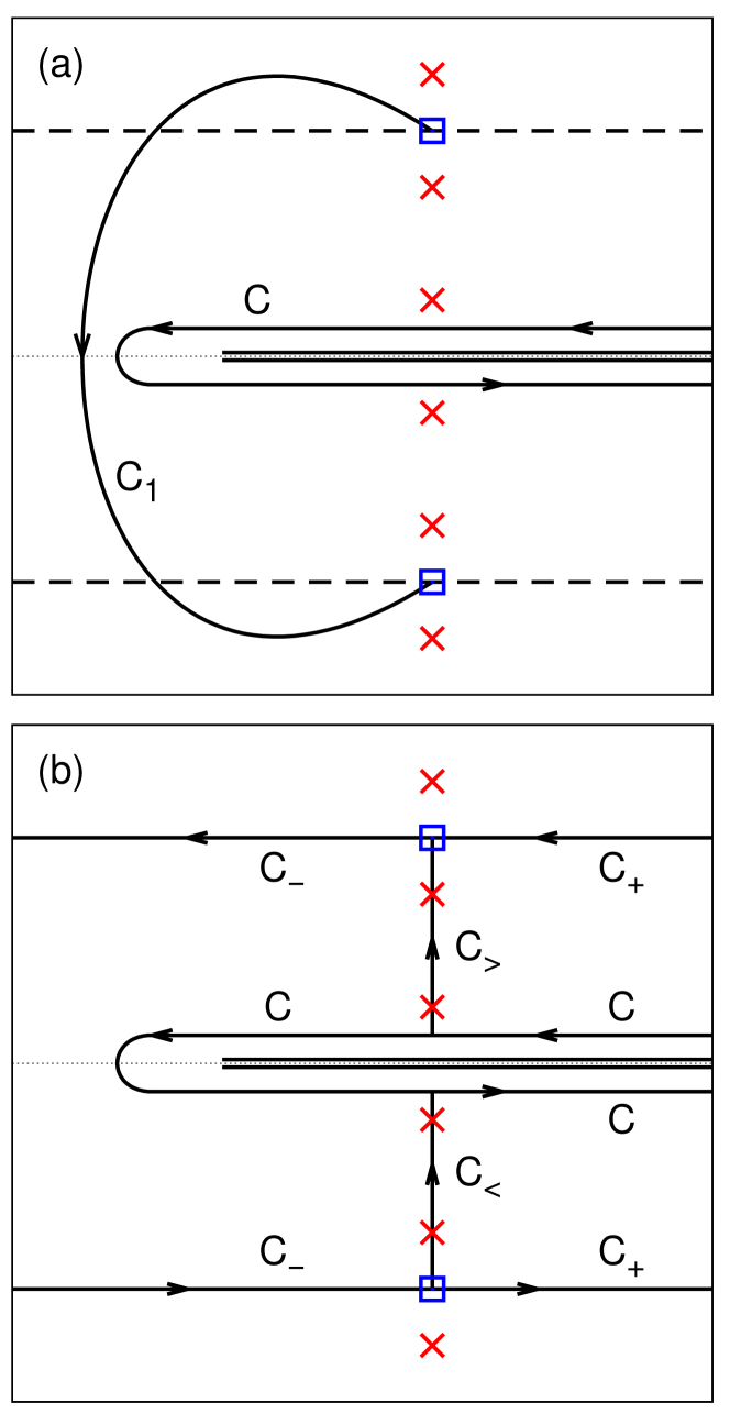
Figure 1: (a) The integration contours $C$ and $C_{1}$ in Eq. (3) and Eq. (5), respectively. The horizontal double line marks the valence part of the spectrum of Hamiltonian $H$, the crosses denote the Matsubara points $z_{k}$ and the squares denote the points $Z_{M}$ and $Z^{\ast}_{M}$ for $M=2$. (b) The integration contours $C$, $C_{+}$, $C_{-}$, $C_{>}$, and $C_{<}$ for entropy calculation.

The standard transformation of Eq. (1) into a complex integral starts from the form

$$Q=\frac{1}{2\pi i}\int_{C}\Gamma(z)f(z)\mathrm{d}z,$$ (3)

where the complex contour $C$ is drawn around the valence part of the spectrum of $H$ as shown in Fig. 1a. The modification of Eq. (3) rests on the well-known properties of the functions $\Gamma(z)$ and $f(z)$, such as their analyticity, the periodicity of $f(z)$ with an imaginary period $2\pi i\beta^{-1}$, the existence of simple poles of $f(z)$ at the Matsubara points $z_{k}=\mu+\pi i\beta^{-1}k$, where $k$ runs over all odd integers, an exponential decay of $f(z)$ for $\Re(z)\to+\infty$, and an exponential decay of $[f(z)-1]$ for $\Re(z)\to-\infty$, where $\Re(z)$ denotes the real part of $z$.

The final form of $Q$, described in the literature Wildberger et al. (1995), employs a point $Z_{M}=\mu+2\pi i\beta^{-1}M$, where $M$ is a positive integer; note that there are exactly $M$ Matsubara points $z_{k}$ lying inside the segment $(\mu,Z_{M})$. This yields:

$$Q=Q_{1}+Q_{2}+Q_{3},$$ (4)

with the individual terms given by

$$Q_{1}=\frac{1}{2\pi i}\int_{C_{1}}\Gamma(z)\mathrm{d}z,$$ (5)

where the contour $C_{1}$ starts at $Z_{M}$ and ends at $Z^{\ast}_{M}$, see Fig. 1a,

$$Q_{2}=\beta^{-1}\sum_{|k|<2M}^{\mathrm{odd}}\Gamma(z_{k}),$$ (6)

where the sum runs over all Matsubara points $z_{k}$ between $Z_{M}$ and $Z^{\ast}_{M}$, and

$$Q_{3} = \frac{i}{2\pi}\int_{-\infty}^{+\infty}\Gamma(Z_{M}+\xi)\,\frac{\mathrm{sign}(\xi)\,\mathrm{d}\xi}{1+\exp(\beta|\xi|)}$$ (7)

$${}-\frac{i}{2\pi}\int_{-\infty}^{+\infty}\Gamma(Z^{\ast}_{M}+\xi)\,\frac{\mathrm{sign}(\xi)\,\mathrm{d}\xi}{1+\exp(\beta|\xi|)},$$

where the integrations over a real variable $\xi$ correspond to complex integrals along the horizontal dashed lines in Fig. 1a. Note that the contributions over $\xi>0$ in Eq. (7) refer to integrations of $f(z)\Gamma(z)$, whereas those over $\xi<0$ refer to integrations of $[f(z)-1]\Gamma(z)$. By employing the rule $\Gamma(z^{\ast})=\Gamma^{\ast}(z)$, the integrations in $Q_{1}$ and $Q_{3}$ and the summation in $Q_{2}$ can be performed with arguments $z$ of $\Gamma(z)$ lying only in the upper (or lower) complex half-plane, see Ref. Wildberger et al., 1995 for more details.

Numerically, the integral in $Q_{1}$ (5) can be evaluated by using a finite number of nodes along the path $C_{1}$ and corresponding weights, and the integrals in $Q_{3}$ (7) can be obtained from a finite number of terms of the Taylor expansion of $\Gamma(z)$ at the point $Z_{M}$. The coefficients of this expansion are obtained from the values of $\Gamma(z)$ in a few points $z$ lying in the neighborhood of $Z_{M}$ and the remaining integrals can be reduced (for odd positive integers $j$) to

$$R_{j}=\int_{-\infty}^{+\infty}\frac{|u|^{j}\,\mathrm{d}u}{1+\mathrm{e}^{|u|}}=2\,j!\,(1-2^{-j})\,\zeta(j+1),$$ (8)

where $\zeta(a)=\sum_{n=1}^{\infty}n^{-a}$ is the Riemann’s zeta-function (for $a>1$).

II.2 Entropy

The entropy corresponding to a positive temperature and the one-particle Hamiltonian $H$ is given by

$$S=k_{\mathrm{B}}\int_{-\infty}^{+\infty}D(E)\sigma(E)\mathrm{d}E,$$ (9)

where $D(E)$ is the total DOS of the system related to the Green’s function (resolvent) by Eq. (2) with $\Gamma(z)=\mathrm{Tr}\{G(z)\}$, and where the function $\sigma(E)$ is defined as

$$\sigma(E)=-f(E)\ln[f(E)]-[1-f(E)]\ln[1-f(E)].$$ (10)

Since complex logarithm is a multivalued function, the real function $\sigma(E)$ can be directly continued analytically into its complex counterpart $\sigma(z)$ only in a stripe around the real energy axis, namely, for $|\Im(z)|<\pi\beta^{-1}$, where $\Im(z)$ denotes the imaginary part of $z$. [Here and below, we assume the branch cut of $\ln(w)$ along the real negative half-axis, $w<0$.] For present purposes, let us define continuations $\sigma_{-}(z)$ and $\sigma_{+}(z)$ of $\sigma(E)$ that are analytic in the entire half-planes $\Re(z)<\mu$ and $\Re(z)>\mu$, respectively:

$$\sigma_{\pm}(z)=\frac{\pm t}{1+\mathrm{e}^{\pm t}}+\ln(1+\mathrm{e}^{\mp t}),\ \quad t=\beta(z-\mu),$$ (11)

and let us discuss briefly their properties. First, the function $\sigma_{+}(z)$ decays exponentially for $\Re(z)\to+\infty$ and the function $\sigma_{-}(z)$ decays exponentially for $\Re(z)\to-\infty$. Second, it can be shown that $\sigma_{+}(z)$ and $\sigma_{-}(z)$ possess the same leading term of their singular behavior near the Matsubara points $z_{k}$:

$$\sigma_{\pm}(z)=(\mu-z_{k})(z-z_{k})^{-1}+\dots,$$ (12)

where the omitted term includes a regular part and a weak (logarithmic) singularity. Third, along the vertical line $z=\mu+i\eta$ ($\eta$ is real), the limits of $\sigma_{\pm}(\mu\pm\varepsilon+i\eta)$ for $\varepsilon\to 0^{+}$ can be considered; their difference equals

$$\tau(\mu+i\eta) = \lim_{\varepsilon\to 0^{+}}[\sigma_{+}(\mu+\varepsilon+i\eta)-\sigma_{-}(\mu-\varepsilon+i\eta)]$$ (13)

$$= 2\pi i\,[[\beta\eta/(2\pi)]],$$

where $[[u]]$ denotes the integer nearest to the real quantity $u$. This result means that $\tau(\mu+i\eta)$ is a piecewise constant function of $\eta$ with discontinuities at $\eta=\pi\beta^{-1}k$, where $k$ is an odd integer (i.e., whenever $\mu+i\eta=z_{k}$). The last property reflects the fact that the derivatives of $\sigma_{+}(z)$ and $\sigma_{-}(z)$ coincide mutually in the whole complex plane except at the Matsubara points $z_{k}$, where second-order poles of both derivatives are located. Fourth, along horizontal lines $z=E+2\pi i\beta^{-1}m$, where $m$ is an integer, it holds

$$\sigma_{\pm}(E+2\pi i\beta^{-1}m)=\sigma(E)\pm\frac{2\pi im}{1+\exp[\pm\beta(E-\mu)]}\,,$$ (14)

proving explicitly that the functions $\sigma_{\pm}(z)$ are not periodic with the period $2\pi i\beta^{-1}$, in contrast to the function $f(z)$.

The expression for the entropy (9) can be written as a complex integral

$$\frac{S}{k_{\mathrm{B}}}=\frac{1}{2\pi i}\int_{C}\Gamma(z)\sigma(z)\mathrm{d}z$$ (15)

along the same path $C$ as in Eq. (3). The deformation of the contour $C$ has to be performed separately on both sides of the vertical line $\Re(z)=\mu$, see Fig. 1b. This leads to the form

$$S=S_{+}+S_{-}+S_{>}+S_{<}$$ (16)

with the individual terms given by

$$\frac{S_{\gtrless}}{k_{\mathrm{B}}} = \frac{i}{2\pi}\int_{C_{\gtrless}}\Gamma(z)\tau(z)\mathrm{d}z+\sum_{|k|<2M}^{k\gtrless 0,\mathrm{odd}}(z_{k}-\mu)\Gamma(z_{k}),$$

$$\frac{S_{\pm}}{k_{\mathrm{B}}} = \frac{1}{2\pi i}\int_{C_{\pm}}\Gamma(z)\sigma_{\pm}(z)\mathrm{d}z,$$ (17)

where the paths $C_{+}$, $C_{-}$, $C_{>}$, and $C_{<}$ are depicted in Fig. 1b and where the functions $\sigma_{\pm}(z)$ (11), $\tau(z)$ (13), and the singular behavior of $\sigma_{\pm}(z)$ (12) have been used.

The contribution $S_{+}$ is calculated from Eq. (14) for $m=M$ and $m=-M$, and similarly for $S_{-}$. This yields together

$$\frac{S_{+}+S_{-}}{k_{\mathrm{B}}}=-\frac{1}{\pi}\int_{-\infty}^{+\infty}\Im[\Gamma(Z_{M}+\xi)]\,\sigma(\mu+\xi)\,\mathrm{d}\xi$$

$${}-2M\int_{-\infty}^{+\infty}\Re[\Gamma(Z_{M}+\xi)]\,\frac{\mathrm{sign}(\xi)\,\mathrm{d}\xi}{1+\exp(\beta|\xi|)}\,.\quad$$ (18)

Numerically, the integrals in Eq. (18) can again be obtained from a finite number of terms of the Taylor expansion of $\Gamma(z)$ at the point $Z_{M}$. The encountered integrals are $R_{j}$ (8) and (for even non-negative integers $j$)

$$N_{j} = \int_{-\infty}^{+\infty}u^{j}\left[\frac{\ln(1+\mathrm{e}^{u})}{1+\mathrm{e}^{u}}+\frac{\ln(1+\mathrm{e}^{-u})}{1+\mathrm{e}^{-u}}\right]\mathrm{d}u$$ (19)

$$= \frac{j+2}{j+1}\,R_{j+1}\,.$$

The evaluation of $S_{>}$ and $S_{<}$ in Eq. (17) is greatly simplified by the fact that the function $\tau(z)$ defined along the paths $C_{>}$ and $C_{<}$ is piecewise constant, see Eq. (13). If we denote by $\Phi(z)$ a primitive function to $\Gamma(z)$, so that $\mathrm{d}\Phi(z)/\mathrm{d}z=\Gamma(z)$, we get

$$\frac{S_{>}}{k_{\mathrm{B}}} = \sum_{0<k<2M}^{\mathrm{odd}}\Phi(z_{k})-M\Phi(Z_{M})$$ (20)

$${}+\sum_{0<k<2M}^{\mathrm{odd}}(z_{k}-\mu)\Gamma(z_{k}),$$

and similarly for $S_{<}$. The primitive function can be chosen to satisfy the rule $\Phi(z^{\ast})=\Phi^{\ast}(z)$; in such a case, one obtains

$$\frac{S_{>}+S_{<}}{k_{\mathrm{B}}} = 2\Re\Bigg{\{}\sum_{0<k<2M}^{\mathrm{odd}}\left[\Phi(z_{k})+(z_{k}-\mu)\Gamma(z_{k})\right]\Bigg{.}$$ (21)

$$\Bigg{.}{}-M\Phi(Z_{M})\Bigg{\}}.$$

This result means that only the values of $\Gamma(z)$ and $\Phi(z)$ at the point $Z_{M}$ and at the $M$ lowest Matsubara points $z_{k}$ in the upper half-plane are needed. In practice, the function $\Phi(z)$ is often constructed as $\Phi(z)=\ln(|z-H|)$, where $|z-H|$ denotes the determinant of the secular matrix. Note that the ambiguity of the imaginary part of logarithm does not affect the obtained result (21), which depends only on the unambiguous real part of the logarithmic function.

Let us conclude this section by a few comments to the derived final expression for the entropy $S$, given by the sum of Eq. (18) and Eq. (21). First, this final result includes no explicit contour integral, so that it is simpler than the final result for quantities $Q$ treated in Section II.1. This feature can be ascribed to different asymptotic behavior of the functions $\sigma(E)$ and $f(E)$: the former decays exponentially for $E\to\pm\infty$, whereas the latter decays only for $E\to+\infty$, but it approaches unity for $E\to-\infty$. Second, the primitive function $\Phi(z)$ in Eq. (21), closely related to the integrated DOS, can be constructed from the determinant of the secular matrix not only in a general theory considered here, but also in the multiple-scattering Korringa-Kohn-Rostoker (KKR) theory Wildberger et al. (1995) or in the LMTO method Turek et al. (1997); Drchal et al. (1996). Moreover, for substitutionally disordered systems treated in the coherent potential approximation (CPA), proper configuration averages of the integrated DOS are available in the literature Gonis (1992); Turek et al. (2000). All these expressions for the primitive function $\Phi(z)$ contain the logarithmic function, but the resulting right-hand side of Eq. (21) is defined unambiguously again. Finally, the additional numerical effort to calculate the entropy is negligible as compared to other computations, since the complex energy arguments involved (which comprise the $M$ lowest Matsubara points $z_{k}$, the point $Z_{M}$, and a few points near $Z_{M}$) enter the self-consistent electron-density calculations as well (see end of Section II.1).

III Numerical implementation

The developed formalism has been implemented on a model level and in the self-consistent scalar-relativistic TB-LMTO method Andersen and Jepsen (1984) in the atomic sphere approximation (ASA) and the CPA Turek et al. (1997). Since the numerical evaluation of the entropy follows closely that of the electron densities and effective potentials, the previous experience has been employed to great extent Wildberger et al. (1995). The integration contour $C_{1}$ (Fig. 1a) was a part of a circle with the center located on the real energy axis; the contour integration was performed numerically by means of 14 nodes (distributed along the upper half of $C_{1}$) and corresponding complex weights. In the illustrating example presented in Section IV, several thousands of $\mathbf{k}$ vectors were used for sampling the irreducible part of the bcc Brillouin zone (BZ) for the first Matsubara point $z_{1}$ (closest to the real chemical potential $\mu$), while reduced numbers of $\mathbf{k}$ vectors were used for the complex energy points more distant from $\mu$.

The coefficients of the Taylor expansions of the functions $\Gamma(z)$ at $z=Z_{M}$ were obtained numerically based on the calculated values in a few points in the distance $\sim\beta^{-1}=k_{\mathrm{B}}T$ from $Z_{M}$. In the simplest models, these coefficients were also set their exact values for the sake of comparison of the effect of both alternatives on the resulting electronic entropy. The degree $\nu$ of the Taylor polynomials was varied in the range $1\leq\nu\leq 8$; however, for practical applications with temperatures not exceeding $\sim 1000$ K, polynomials with $\nu\leq 4$ seem to be sufficient in most cases.

IV Results and discussion

We start the discussion of accuracy of the developed formalism for electronic entropy with analysis of a simple model DOS corresponding to an isolated eigenvalue $E_{0}$ which coincides with the chemical potential ($E_{0}=\mu$), so that $D(E)=\delta(E-\mu)$, which yields $\Gamma(z)=(z-\mu)^{-1}$, and $\Phi(z)=\ln(z-\mu)$. We assume that $\mu$ is independent of temperature $T$, which leads to the exact entropy $S_{\mathrm{x}}$ that is $T$-independent as well, $S_{\mathrm{x}}=k_{\mathrm{B}}\ln 2$. A closer look at Eq. (18) and Eq. (21) in this case reveals that they also provide $T$-independent values of the approximate entropy $S$, which thus depends only on two integers $M$ (number of the Matsubara points) and $\nu$ (degree of the Taylor expansion polynomial).

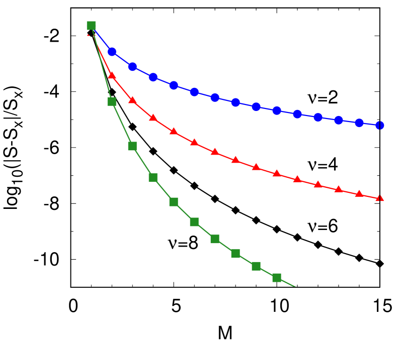
Figure 2: Relative deviations of the calculated entropy $S$ with respect to the exact value $S_{\mathrm{x}}=k_{\mathrm{B}}\ln 2$ for the isolated eigenvalue $E_{0}=\mu$ and for different degrees $\nu$ of the Taylor polynomial as functions of the number $M$ of Matsubara points. Note the logarithmic scale on the vertical axis.

The relative difference between $S$ and $S_{\mathrm{x}}$ is displayed in Fig. 2 as a function of $M$ for several values of $\nu$. One can see that the accuracy of the approximate scheme is quite high, the only exceptions being the cases with very small $M$ or $\nu$. The studied model is very simple indeed; note however that an isolated eigenvalue belongs to the strongest singularities to be encountered in the electronic spectra.

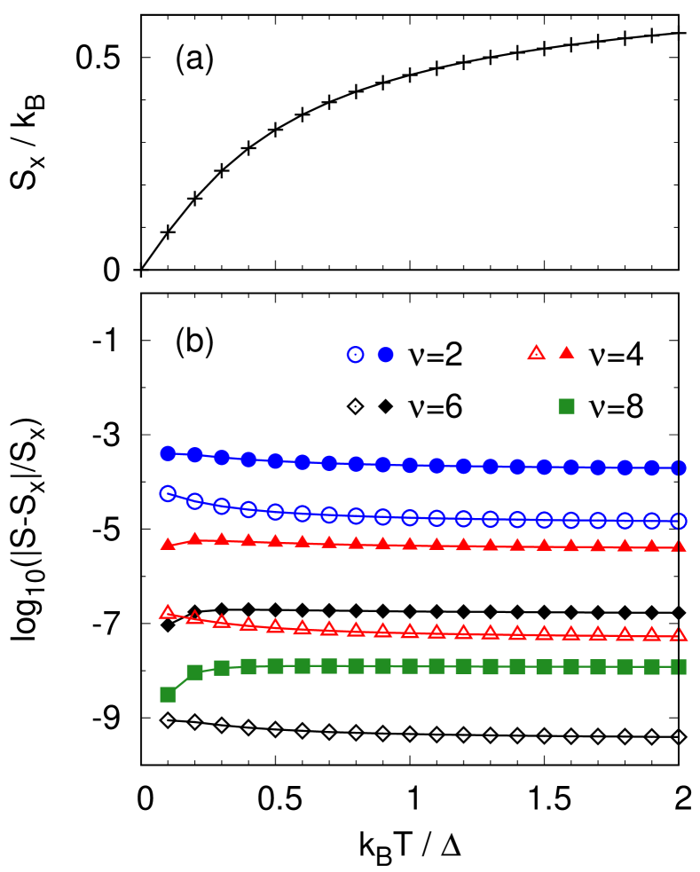
Figure 3: (a) The temperature dependence of the exact entropy $S_{\mathrm{x}}$ for a model Lorentzian DOS of width $\Delta$, see text for details. (b) Relative deviations of the calculated entropy $S$ with respect to $S_{\mathrm{x}}$ as functions of temperature for different degrees $\nu$ of the Taylor polynomial and for two values of the number $M$ of Matsubara points: $M=5$ (solid symbols) and $M=12$ (open symbols).

Another simple model is described by a Lorentzian DOS parametrized by its center $E_{0}$ and width $\Delta$, so that $D(E)\propto[(E-E_{0})^{2}+\Delta^{2}]^{-1}$ and, consequently, $\Gamma(z)=(z-E_{0}+i\Delta)^{-1}$ and $\Phi(z)=\ln(z-E_{0}+i\Delta)$ for $\Im(z)>0$. We have chosen a slight offset of the center $E_{0}$ with respect to the chemical potential $\mu$, namely, $E_{0}-\mu=0.4\Delta$, and have assumed all parameters ($E_{0}$, $\Delta$, $\mu$) as $T$-independent. The exact entropy $S_{\mathrm{x}}$, obtained by a highly accurate real-energy numerical quadrature according to Eq. (9), is shown in Fig. 3a as a function of $T$. The temperature dependence of the relative difference between the approximate $S$ and the exact $S_{\mathrm{x}}$ is presented in Fig. 3b for two values of $M$ ($M=5$ and $M=12$) and for several values of $\nu$. One can see that the relative deviations are essentially independent of $T$, despite the pronounced increase of the entropy with increasing temperature. One can also observe an increase in the relative accuracy due to higher values of $M$ and $\nu$, indicating that modest numbers $M$ and $\nu$ are sufficient for practical applications of the developed formalism.

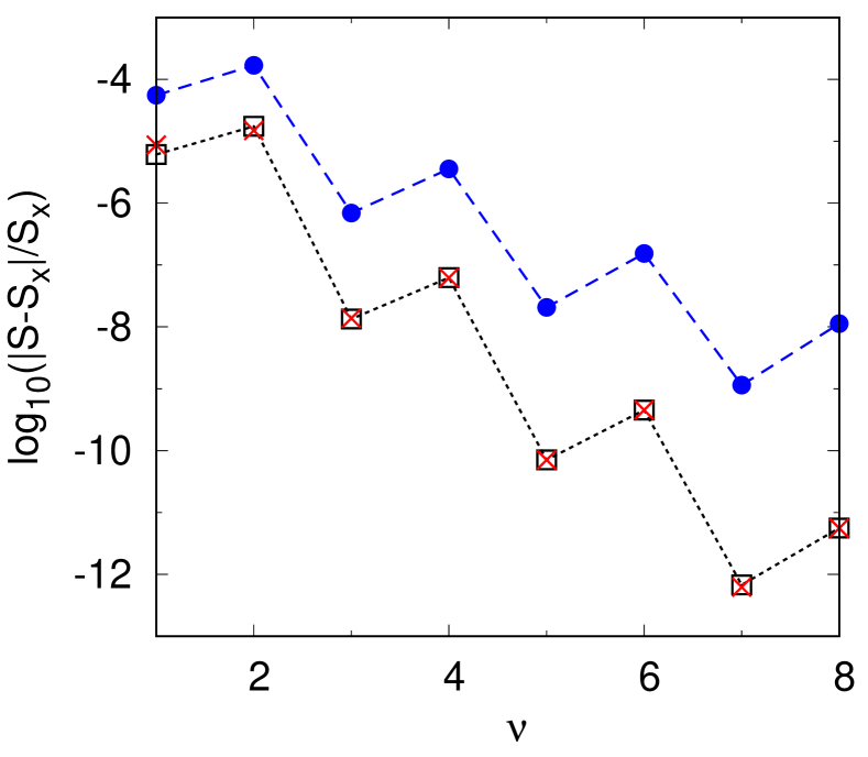
Figure 4: Relative deviations of the calculated entropy $S$ with respect to the corresponding exact value $S_{\mathrm{x}}$ as functions of the degree $\nu$ of the Taylor polynomial: for the isolated eigenvalue with $M=5$ (solid circles) and for the Lorentzian DOS with $k_{\mathrm{B}}T=\Delta$ and $M=12$ (open boxes). The red crosses mark deviations obtained in the latter case with the Taylor expansion coefficients extracted by a numerical procedure.

The origin of numerical inaccuracy in the present evaluation of the entropy can easily be identified (disregarding the well-known convergence issues with respect to the BZ sampling): it is the treatment of integrations in Eq. (18) by using the Taylor expansion polynomials. Note that the same source of inaccuracy refers also to the quantity $Q_{3}$ (7). There are two particular questions related to this point, namely, (i) the effect of the finite degree $\nu$ of the Taylor polynomial, and (ii) the role of the numerical procedure to extract the coefficients of the polynomial. The results found for the above simple models and presented in Fig. 4 provide a partial answer to both questions. First, it is seen that the increase in $\nu$ reduces in general the relative deviations of entropy, but the obtained trends are not strictly monotonic. Second, the numerically obtained coefficients lead essentially to the same values of $S$ as the exact coefficients (see the values marked by red crosses and open boxes in Fig. 4).

These facts represent undoubtedly positive features of the presented formalism from the practical point of view; however, certain caution is needed in attempts to increase the accuracy by using too high degrees $\nu$. First, the convergence radius of the Taylor series of $\Gamma(Z_{M}+\xi)$ is inevitably finite due to the branch cuts (and possible poles) of $\Gamma(z)$ on the real energy axis. This means that there is no strict convergence of $S$ to $S_{\mathrm{x}}$ for $\nu\to\infty$, at least for a fixed number $M$ of the Matsubara points. Second, the procedure to extract the Taylor coefficients from several values of the function $\Gamma(z)$ in neighborhood of $z=Z_{M}$ leads to a set of $\nu$ linear equations for $\nu$ unknown variables. This linear problem (Vandermonde system) is ill-conditioned Press et al. (1992) which can prevent its stable numerical solution for large values of $\nu$.

Table 1: Calculated local magnetic moment $M_{\mathrm{Fe}}$ and electronic entropy $S$ (per atom) for three temperatures $T$ in the DLM state of bcc Fe. The values of $M_{\mathrm{Fe}}$ in parenthesis are from Ref. Ruban et al., 2013.

$T$ (K)	$M_{\mathrm{Fe}}$ ($\mu_{\mathrm{B}}$)	$S/k_{\mathrm{B}}$
0	2.02 (1.96)	0.00
2000	1.92 (1.85)	0.89
4000	1.41 (1.30)	2.09

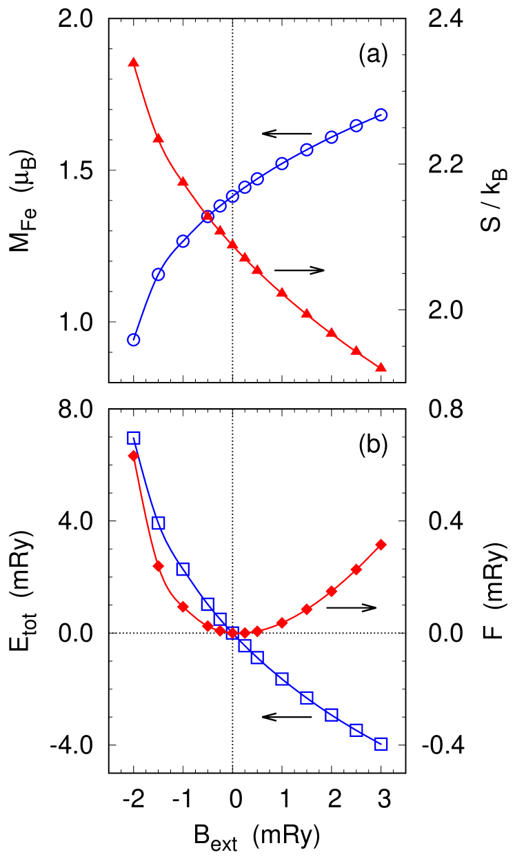
Figure 5: Calculated dependence of various quantities on the random external magnetic field $B_{\mathrm{ext}}$ for bcc Fe in the DLM state at $T=4000$ K: (a) the local magnetic moment $M_{\mathrm{Fe}}$ (open circles) and the electronic entropy $S$ (solid triangles), and (b) the total energy $E_{\mathrm{tot}}$ (open boxes) and the free energy $F$ (solid diamonds). The quantities $S$, $E_{\mathrm{tot}}$ and $F$ are given per one atom; the vertical scales in panel (b) have been shifted to a common zero at $B_{\mathrm{ext}}=0$.

As an illustrating application to a realistic system, we have considered bcc iron in the disordered-local-moment (DLM) state Gyorffy et al. (1985). This system at very high temperatures (up to $T=6000$ K) and under strong pressures attracts ongoing interest in the context of physical properties of the Earth’s core Belonoshko et al. (2017); Ruban et al. (2013); Pozzo and Alfè (2016); Drchal et al. (2017). Here we focus only on the effect of elevated temperatures and treat thus bcc iron of a density corresponding to ambient conditions (Wigner-Seitz radius $s=2.65$ a.u.) within the local spin-density approximation with the local exchange-correlation potential parametrized according to Ref. Vosko et al., 1980. The valence $spdf$-basis was used in the TB-LMTO-ASA method and the CPA; the degree of the Taylor expansion polynomial was set to $\nu=6$. For the very high temperatures considered here, small numbers of the Matsubara points were sufficient: we set $M=8$ for $T=2000$ K and $M=4$ for $T=4000$ K. Calculated values of the self-consistent local magnetic moments $M_{\mathrm{Fe}}$ and of the electronic entropy $S$ (per atom) are shown in Table 1 for three selected temperatures. One can see a sizeable reduction of the local moment due to increasing temperature as expected; the values of $M_{\mathrm{Fe}}$ in this work are slightly higher than the values reported in Ref. Ruban et al., 2013. The electronic entropy increases with increasing temperature, which is another expected trend of finite-temperature behavior.

In order to make better assessment of internal consistence of the formulated entropy $S$ with other electronic quantities, such as the electron densities, local magnetic moments $M_{\mathrm{Fe}}$ and total energies $E_{\mathrm{tot}}$, we have studied these quantities as functions of a randomly oriented external magnetic field $B_{\mathrm{ext}}$ coupled to the electron spin. [For simplicity, the quantity $B_{\mathrm{ext}}$ includes the Bohr magneton $\mu_{\mathrm{B}}$, so that $\pm B_{\mathrm{ext}}$ describes the spin-dependent shift added to the spin-polarized exchange-correlation potential.] The application of this random external field is equivalent to an effect of the constraint in the fixed-spin-moment method applied to the DLM state Drchal et al. (2017). Various calculated quantities for the case of $T=4000$ K are displayed in Fig. 5. One can observe that the magnetic moment $M_{\mathrm{Fe}}$, the entropy $S$, and the total energy $E_{\mathrm{tot}}$ are monotonic functions of the external field $B_{\mathrm{ext}}$ throughout the studied range. However, the free energy $F=E_{\mathrm{tot}}-TS$ exhibits a clear minimum at $B_{\mathrm{ext}}=0$, which represents a necessary condition for an internally consistent theory at finite temperatures. Note that the total energy $E_{\mathrm{tot}}$ is expressed only in terms of quantities discussed in Section II.1, i.e., it is fully independent of the treatment of the electronic entropy $S$ described in Section II.2.

V Conclusion

We have revised the evaluation of physical quantities in finite-temperature Green’s-function techniques with particular attention paid to the electronic entropy. We have shown that usual obstacles encountered in entropy calculations (branch cuts or ambiguity of complex logarithm) can be removed completely, which leads to a simple final expression without an explicit contour integration. The final result can be implemented both in semiempirical TB schemes as well as in ab initio Green’s function approaches based on the KKR or the LMTO methods, optionally also with the CPA for chemically disordered systems. The finite numerical accuracy of the developed formalism, which is due to a standard auxiliary Taylor expansion of the resolvent, seems to be well under control. The electronic entropy thus need not be avoided in Green’s function techniques, but it should rather be employed directly for reliable computations of other thermodynamic potentials.