Exponentially Consistent Kernel Two-Sample Tests

Abstract

Given two sets of independent samples from unknown distributions $P$ and $Q$, a two-sample test decides whether to reject the null hypothesis that $P=Q$. Recent attention has focused on kernel two-sample tests as the test statistics are easy to compute, converge fast, and have low bias with their finite sample estimates. However, there still lacks an exact characterization on the asymptotic performance of such tests, and in particular, the rate at which the type-II error probability decays to zero in the large sample limit. In this work, we establish that a class of kernel two-sample tests are exponentially consistent with Polish, locally compact Hausdorff sample space, e.g., $\mathbb{R}^{d}$. The obtained exponential decay rate is further shown to be optimal among all two-sample tests satisfying the level constraint, and is independent of particular kernels provided that they are bounded continuous and characteristic. Our results gain new insights into related issues such as fair alternative for testing and kernel selection strategy. Finally, as an application, we show that a kernel based test achieves the optimal detection for off-line change detection in the nonparametric setting.

1 Introduction

Given two sets of i.i.d. samples, the two-sample problem decides whether or not to accept the null hypothesis that the generating distributions are the same, without imposing any parametric assumptions. This is important to a variety of applications, including data integration in bioinformatics [4], statistical model criticism [19, 24], and training deep generative models [11, 20, 22, 31]. Typical two-sample tests are constructed based on some distance measures between distributions, such as classical Kolmogorov-Smirnov distance [12], Kullback-Leibler divergence (KLD) [5, 26], and maximum mean discrepancy (MMD), a reproducing kernel Hilbert space norm of the difference between kernel mean embeddings of distributions [15, 16, 25, 28, 35]. Notably, kernel based test statistics possess several key advantages such as computational efficiency and fast convergence, thereby attracting much attention recently.

A hypothesis test is usually evaluated by characterizing its type-II error probability subject to a level constraint on the type-I error probability. In this respect, existing kernel two-sample tests have been shown to be consistent, in the sense that the type-II error probability decreases to zero as sample sizes scale to infinity. While consistency is a desired property, quantifying how fast the error probability decays is even more desirable, as it provides a natural metric for comparing test performance. However, exact characterization on the decay rate is still elusive, even for some well-known kernel two-sample tests. For example, assuming $n$ samples in both sets, the decay rate of the biased quadratic-time test in [15] is claimed to be (at least) $\mathcal{O}(n^{-0.5})$, based on a large deviation bound on the test statistic. The large deviation bound has been observed to be loose in general, indicating that the above decay rate is loose too. Other works such as [16, 31, 35] have established the limiting distributions of the test statistics, but they also do not give a tight decay rate. Clearly, no statistical optimality can be claimed if the characterization itself is loose.

More recently, in the context of goodness of fit testing, Zhu et al. [36] showed that the quadratic-time kernel two-sample tests have the type-II error probability vanishing exponentially fast at a rate determined by the KLD between the two generating distributions. A strong condition for this result is that sample sizes need scale in different orders. Their approach, however, is not readily applicable when sample sizes increase in the same order, e.g., when the two sets have an equal number of samples. This is because existing Sanov’s theorems only hold for the sample sequence originating from one given distribution, whereas the acceptance region defined by the kernel two-sample test involves two sample sequences from different distributions. As such, the key seems to be an extended version of Sanov’s theorem that handles two distributions; this is not apparent as existing tools, e.g., Cramér theorem [9] that is used for proving Sanov’s theorem, can only deal with a single distribution.

The first goal of this paper is to seek an exact statistical characterization for a widely used kernel two-sample test. We establish an extended version of Sanov’s theorem w.r.t. the topology induced by a pairwise weak convergence of probability measures. Our proof is inspired by Csiszár [8] which proved original Sanov’s theorem of one sample sequence in the $\tau$-topology. Based on the idea of [36], we then show that the biased quadratic-time kernel two-sample test in [15] is exponentially consistent when sample sizes scale in the same order. The obtained exponential decay rate depends only on the generating distributions and the samples sizes under the alternative hypothesis, and is further shown to be the optimal one among all two-sample tests satisfying the level constraint. A notable implication is that kernels affect only the sub-exponential term in the type-II error probability, provided that they are bounded continuous and characteristic. We also comment that the extended Sanov’s theorem may be of independent interest and may be applied to other large deviation applications.

Our second goal is to derive an optimality criterion for nonparametric two-sample tests as well as a way of finding more tests achieving this optimality. Towards this goal, we characterize the maximum exponential decay rate for any two-sample test under the given level constraint. Furthermore, a sufficient condition is derived for the type-II error probability to decay at least exponentially fast with the maximum exponential rate (possibly violating the level constraint). These results provide new insights into related issues such as fair alternative for testing and kernel selection strategy, which are elaborated in Sections 3.4 and 5. As an application, we apply our results to the off-line change detection problem and show that a kernel based test achieves the optimal detection in terms of the exponential decay rate of the type-II error probability. To our best knowledge, this is the first time that a test is shown to be optimal for detecting the presence of a change in the nonparametric setting.

In Section 2, we briefly review the MMD and the two-sample testing. In Section 3, we present our main results on the exact and optimal exponential decay rate for a class of kernel two-sample tests, followed by discussions on related issues. We apply our results to off-line change detection in Section 4 and conduct synthetic experiments in Section 5. Section 6 concludes the paper.

2 Maximum mean discrepancy, two-sample testing, and test threshold

We briefly review the MMD and its weak metrizable property. We then describe the two-sample problem as statistical hypothesis testing and choose a suitable threshold for the level constraint.

Maximum mean discrepancy

Let $\mathcal{F}$ be a reproducing kernel Hilbert space (RKHS) defined on a topological space $\mathcal{X}$ with reproducing kernel $k$. Let $x$ be an $\mathcal{X}$-valued random variable with probability measure $P$, and $\mathbf{E}_{x}f(x)$ the expectation of $f(x)$ for a function $f:\mathcal{X}\to\mathbb{R}$. Assume that $k$ is bounded continuous. Then for every Borel probability measure $P$ defined on $\mathcal{X}$, there exists a unique element $\mu_{k}(P)\in\mathcal{F}$ such that $\mathbf{E}_{x}f(x)=\langle f,\mu_{k}(P)\rangle_{\mathcal{F}}$ for all $f\in\mathcal{F}$ [3]. The MMD between two Borel probability measures $P$ and $Q$ is the RKHS-distance between $\mu_{k}(P)$ and $\mu_{k}(Q)$, which can be expressed as

$$d_{k}(P,Q)=\|\mu_{k}(P)-\mu_{k}(Q)\|_{\mathcal{F}}=\left(\mathbf{E}_{x,x^{\prime}}k(x,x^{\prime})+\mathbf{E}_{y,y^{\prime}}k(y,y^{\prime})-2\mathbf{E}_{x,y}k(x,y)\right)^{1/2},$$

where $x,x^{\prime}$ i.i.d. $\sim P$ and $y,y^{\prime}$ i.i.d. $\sim Q$ [15]. If the kernel $k$ is characteristic, then $d_{k}(P,Q)=0$ if and only if $P=Q$ [30]. This property enables the MMD to distinguish different distributions.

We present a weak metrizable property of $d_{k}$, which will be used to establish our main results in Section 3. Let $\mathcal{P}$ denote the set of all Borel probability measures defined on $\mathcal{X}$. For a sequence of probability measures $P_{l}\in\mathcal{P}$, we say that $P_{l}\to P$ weakly if and only if $\mathbf{E}_{x\sim P_{l}}f(x)\to\mathbf{E}_{x\sim P}f(x)$ for every bounded continuous function $f:\mathcal{X}\to\mathbb{R}$.

Theorem 1 ([28, 29]).

The MMD $d_{k}(\cdot,\cdot)$ metrizes the weak convergence on $\mathcal{P}$ if the following two conditions hold: (A1) the sample space $\mathcal{X}$ is Polish, locally compact and Hausdorff; (A2) the kernel $k$ is bounded continuous and characteristic.

We note that the weak metrizable property is also favored for training deep generative models [1, 20]. An example of Polish, locally compact Hausdorff space is $\mathbb{R}^{d}$, and the Gaussian kernel satisfies the conditions of A2.

Two-sample testing based on the MMD

Let $x^{n}$ and $y^{m}$ be independent samples, with $x^{n}\sim P$ and $y^{m}\sim Q$ where $P$ and $Q$ are unknown. The two-sample testing is to decide between $H_{0}:P=Q$ and $H_{1}:P\neq Q$. Let $\hat{P}_{n}$ and $\hat{Q}_{m}$ be the respective empirical measures of $x^{n}$ and $y^{m}$, that is, $\hat{P}_{n}=\frac{1}{n}\sum_{i=1}^{n}\delta_{x_{i}}$ and $\hat{Q}_{m}=\frac{1}{m}\sum_{i=1}^{m}\delta_{y_{i}}$ with $\delta_{x}$ being Dirac measure at $x$. Then the squared MMD can be estimated by

$$d_{k}^{2}(\hat{P},\hat{Q})=\frac{1}{n^{2}}\sum_{i=1}^{n}\sum_{j=1}^{n}k(x_{i},x_{j})+\frac{1}{m^{2}}\sum_{i=1}^{m}\sum_{j=1}^{m}k(y_{i},y_{j})-\frac{2}{nm}\sum_{i=1}^{n}\sum_{j=1}^{m}k(x_{i},y_{j}),$$

which is a biased statistic originally proposed in [15]. A hypothesis test for the two-sample testing can then be constructed by comparing this statistic with a threshold $\gamma_{n,m}$: if $d_{k}(\hat{P}_{n},\hat{Q}_{m})\leq\gamma_{n,m}$, then the test accepts the null hypothesis $H_{0}$. The acceptance region is hence defined as $\mathcal{A}(n,m)=\{(x^{n},y^{m}):d_{k}(\hat{P}_{n},\hat{Q}_{m})\leq\gamma_{n,m}\}$. There are two types of errors: a type-I error is made if $(x^{n},y^{m})\notin\mathcal{A}(n,m)$ despite $H_{0}:P=Q$ being true, and a type-II error occurs when $(x^{n},y^{m})\in\mathcal{A}(n,m)$ under $H_{1}:P\neq Q$. The type-I and type-II error probabilities are given by

$$\alpha_{n,m} =\mathbf{P}_{x^{n}y^{m}}\left((x^{n},y^{m})\notin\mathcal{A}(n,m)\right)~{}\text{under}~{}H_{0}:P=Q,$$

$$\beta_{n,m} =\mathbf{P}_{x^{n}y^{m}}\left((x^{n},y^{m})\in\mathcal{A}(n,m)\right)~{}\text{under}~{}H_{1}:P\neq Q,$$

respectively. Bear in mind that $\alpha_{n,m}$ and $\beta_{n,m}$ are computed w.r.t. the true yet unknown distributions.

With a carefully chosen threshold, the above kernel test has been shown to be consistent in [15]. That is, $\beta_{n,m}\to 0$ as $n,m\to\infty$, while $\alpha_{n,m}\leq\alpha$ with $\alpha\in(0,1)$ being set in advance. In this paper, we study the exponential decay rate of $\beta_{n,m}$ in the large sample limit, subject to the same level constraint. Specifically, we aim to characterize

$$\liminf_{n,m\to\infty}-\frac{1}{n+m}\log\beta_{n,m},~{}\text{subject to}~{}\alpha_{n,m}\leq\alpha.$$

The above limit is also called the type-II error exponent in information theory [7]. If the limit is positive, then the test is said to be exponentially consistent.

A suitable threshold

We directly use a result from [15] in order to pick a proper threshold for the level constraint $\alpha_{n,m}\leq\alpha$. Such tests are referred to as level $\alpha$ tests in statistics [6].

Lemma 1 ([15, Theorem 7]).

Let $P$, $Q$, $x^{n}$, $y^{m}$, $\hat{P}_{n}$, $\hat{Q}_{m}$ be defined as in Section 2, and assume A2 with $K$ being a positive upper bound on $k(\cdot,\cdot)$. Then under the null hypothesis $H_{0}:P=Q$,

$$\mathbf{P}_{x^{n}y^{m}}\left(d_{k}(\hat{P}_{n},\hat{Q}_{m})>2(K/m)^{\frac{1}{2}}+2(K/n)^{\frac{1}{2}}+\epsilon\right)\leq 2\exp\left(-\frac{\epsilon^{2}mn}{2K(m+n)}\right).$$

Therefore, for a given $0<\alpha<1$, choosing

$$\gamma_{n,m}=\left((K/m)^{\frac{1}{2}}+(K/n)^{\frac{1}{2}}\right)\left(2+\sqrt{2\log(2\alpha^{-1})}\right),$$ (1)

the kernel test $d_{k}(\hat{P}_{n},\hat{Q}_{m})\leq\gamma_{n,m}$ has its type-I error probability $\alpha_{n,m}<\alpha$, hence is a level $\alpha$ test.

3 Main results

In this section, we present our main results on the type-II error exponent of a class of kernel two-sample tests. The first and the most important step is to establish an extended Sanov’s theorem that works with two sample sequences.

3.1 Extended Sanov’s theorem

We define a pairwise weak convergence: we say $(P_{l},Q_{l})\to(P,Q)$ weakly if and only if both $P_{l}\to P$ and $Q_{l}\to Q$ weakly. We consider $\mathcal{P}\times\mathcal{P}$ endowed with the topology induced by this pairwise weak convergence. It can be verified that this topology is equivalent to the product topology on $\mathcal{P}\times\mathcal{P}$ where each $\mathcal{P}$ is endowed with the topology of weak convergence. An extended version of Sanov’s theorem is given below.

Theorem 2 (Extended Sanov’s Theorem).

Let $\mathcal{X}$ be a Polish space, $x^{n}$ i.i.d. $\sim P$, and $y^{m}$ i.i.d. $\sim Q$. Assume $0<\lim_{n,m\to\infty}\frac{n}{n+m}=c<1$. Then for a set $\Gamma\subset\mathcal{P}\times\mathcal{P}$, it holds that

$$\limsup_{n,m\to\infty}-\frac{1}{n+m}\log\mathbf{P}_{x^{n}y^{m}}((\hat{P}_{n},\hat{Q}_{m})\in\Gamma) \leq\inf_{(R,S)\in\operatorname{int}\Gamma}cD(R\|P)+(1-c)D(S\|Q),$$

$$\liminf_{n,m\to\infty}-\frac{1}{n+m}\log\mathbf{P}_{x^{n}y^{m}}((\hat{P}_{n},\hat{Q}_{m})\in\Gamma) \geq\inf_{(R,S)\in\operatorname{cl}\Gamma}cD(R\|P)+(1-c)D(S\|Q),$$

where $\operatorname{int}$ and $\operatorname{cl}$ denote the interior and closure w.r.t. the pairwise weak convergence, respectively.

We prove the above result in finite sample space and then extend it to general Polish space, with two simple combinatorial lemmas as prerequisites. See details in Appendix A.

3.2 Exact exponent of type-II error probability

With the extended Sanov’s theorem and a vanishing threshold $\gamma_{n,m}$ given in Eq. (1), we are ready to establish the exponential decay of the type-II error probability. Our result follows.

Theorem 3.

Assume A1, A2, and $\lim_{n,m\to\infty}\frac{n}{n+m}=c\in(0,1)$. Under the alternative hypothesis $H_{1}:P\neq Q$, also assume that

$$0<D^{*}:=\inf_{R\in\mathcal{P}}cD(R\|P)+(1-c)D(R\|Q)^{*}<\infty.$$

Given $0<\alpha<1$, the kernel test $d_{k}(\hat{P}_{n},\hat{Q}_{m})\leq\gamma_{n,m}$ with $\gamma_{n,m}$ in Eq. (1) is an exponentially consistent level $\alpha$ test:

$$\alpha_{n,m}\leq\alpha,~{}\text{and}~{}\liminf_{n,m\to\infty}-\frac{1}{n+m}\log\beta_{n,m}=D^{*}.$$

Proof.

We use the fact that testing if $(x^{n},y^{m})\in\{(x^{n},y^{m}):d_{k}(\hat{P}_{n},\hat{Q}_{m})\leq\gamma_{n,m}\}$ is equivalent to testing if $(\hat{P}_{n},\hat{Q}_{m})\in\{(P^{\prime},Q^{\prime}):d_{k}(P^{\prime},Q^{\prime})\leq\gamma_{n,m}\}$. Since the threshold $\gamma_{n,m}\to 0$ as $n,m\to\infty$, $\gamma_{n,m}$ is eventually smaller than any fixed $\gamma>0$, and hence $\{(P^{\prime},Q^{\prime}):d_{k}(P^{\prime},Q^{\prime})\leq\gamma_{n,m}\}\subset\{(P^{\prime},Q^{\prime}):d_{k}(P^{\prime},Q^{\prime})\leq\gamma\}$ for large enough $n,m$. By the extended Sanov’s theorem, the type-II error probability decays at least exponentially fast if $(P,Q)\notin\operatorname{cl}(\{(P^{\prime},Q^{\prime}):d_{k}(P^{\prime},Q^{\prime})\leq\gamma\})$, which can be satisfied by picking $\gamma<d_{k}(P,Q)$ under $H_{1}:P\neq Q$ and using the weak convergence property of the MMD (cf. Theorem 1). We then show that the exponential decay rate is both lower bounded and upper bounded by $D^{*}$ based on the lower semi-continuity of the KLD [34] and Stein’s lemma [9], respectively. Details can be found in Appendix B. ∎

Therefore, when $0<c<1$, the type-II error probability vanishes as $\mathcal{O}(e^{-(n+m)(D^{*}-\epsilon)})$, where $\epsilon\in(0,D^{*})$ is fixed and can be arbitrarily small. The result also shows that kernels only affect the sub-exponential term in the type-II error probability, provided that they meet the conditions of A2.

Not covered in Theorem 3 is the case when $n$ and $m$ scale in different orders, i.e., when $c=0$ or $1$. Without loss of generality, we may consider only $c=1$, with $\lim_{n,m\to\infty}{n}/{m}\to\infty$. If $0<D(P\|Q)<\infty$ under the alternative hypothesis, then [36, Theorem 4] indicates that

$$\liminf_{n,m\to\infty}-\frac{1}{m}\log\beta_{n,m}=D(P\|Q),$$ (2)

which leads to a degenerate result on the error exponent w.r.t. the sample size $n+m$:

$$\liminf_{n,m\to\infty}-\frac{1}{n+m}\log\beta_{n,m}=\liminf_{n,m\to\infty}\frac{1}{1+\frac{n}{m}}\left(-\frac{1}{m}\log\beta_{n,m}\right)=0.$$

Notice that, with $c=1$ (and $0$) we have $D^{*}=0$. Then Theorem 3 still holds if we remove the assumption $c\in(0,1)$. However, the error exponent being $0$ also includes the case where $\beta_{n,m}$ is bounded away from $0$. The more insightful perspective is to look at Eq. (2), and the test is said to be exponentially consistent w.r.t. the sample size $m$.

3.3 Optimal exponent and more exponentially consistent two-sample tests

We can identify other two-sample tests that are at least exponentially consistent based on the above results. In particular, the lower bounds still hold if another test has a smaller type-II error probability, or if $\mathbf{P}_{x^{n}y^{m}}(\mbox{${\cal A}$}^{\prime}(n,m))\leq\mathbf{P}_{x^{n}y^{m}}(\mbox{${\cal A}$}(n,m))$ under $H_{1}:P\neq Q$, where $\mathcal{A}^{\prime}(n,m)$ is the acceptance region defined by the test. A special case is considered in the following theorem, directly from Theorem 3 and Eq. (2).

Theorem 4.

Let $\mathcal{X}$, $x^{n}$, $y^{m}$, $P$, $Q$, $\hat{P}$, $\hat{Q}$, and $D^{*}$ be defined as in Theorem 3. Assume A1 and A2. Let $\mbox{${\cal A}$}^{\prime}(n,m)$ be the acceptance region of another two-sample test and $\beta^{\prime}_{n,m}$ the type-II error probability. If $\mbox{${\cal A}$}^{\prime}(n,m)\subset\{(x^{n},y^{m}):d_{k}(\hat{P}_{n},\hat{Q}_{m})\leq\gamma^{\prime}_{n,m}\}$ where $\gamma^{\prime}_{n,m}\to 0$ as $n,m\to\infty$, then

$$\liminf_{n,m\to\infty}-\frac{1}{n+m}\log\beta^{\prime}_{n,m}\geq D^{*},$$

when $0<\lim_{n,m\to\infty}\frac{n}{n+m}=c<1$ and $0<D^{*}<\infty$; and

$$\liminf_{n,m\to\infty}-\frac{1}{m}\log\beta^{\prime}_{n,m}\geq D(P\|Q),$$

when $\lim_{n,m\to\infty}\frac{n}{m}=\infty$ and $0<D(P\|Q)<\infty$.

The above theorem characterizes only the type-II error exponent. A suitable threshold is needed to guarantee the test be level $\alpha$ for practical use. Our next result provides an upper bound on the optimal type-II error exponent of any (asymptotically) level $\alpha$ test.

Theorem 5.

Let $x^{n}$, $y^{m}$, $P$, $Q$, and $D^{*}$ be defined as in Theorem 4. For a test $\mbox{${\cal A}$}^{\prime}(n,m)$ which is (asymptotically) level $\alpha,0<\alpha<1$, its type-II error probability $\beta^{\prime}_{n,m}$ satisfies

$$\liminf_{n,m\to\infty}-\frac{1}{n+m}\log\beta^{\prime}_{n,m}\leq D^{*},$$

if $0<\lim_{n,m\to\infty}\frac{n}{n+m}=c<1$ and $0<D^{*}<\infty$; and

$$\liminf_{n,m\to\infty}-\frac{1}{m}\log\beta^{\prime}_{n,m}\leq D(P\|Q),$$

if $\lim_{n,m\to\infty}\frac{n}{m}=\infty$ and $0<D(P\|Q)<\infty$.

Proof.

Let $P^{\prime}$ be such that $cD(P^{\prime}\|P)+(1-c)D(P^{\prime}\|Q)=D^{*}$ for $0<c<1$. Define $A_{n}=\{x^{n}:|\frac{1}{n}\log\frac{dP^{\prime}(x^{n})}{dP(x^{n})}-D(P^{\prime}\|P)|\leq\epsilon\}$, and $B_{m}=\{y^{m}:|\frac{1}{m}\log\frac{dP^{\prime}(y^{m})}{dQ(y^{m})}-D(P^{\prime}\|Q)|\leq\epsilon\}$, where $\epsilon>0$ is fixed and can be arbitrary. Here ${dP^{\prime}}/{dP}$ and ${dP^{\prime}}/{dQ}$ are Radon-Nikodym derivatives and exist by the finiteness of $D^{*}$. Consider the acceptance region $A_{n}\times B_{m}\cap\mbox{${\cal A}$}^{\prime}(n,m)$, from which we can obtain an upper bound $D^{*}+\epsilon$ on the type-II error exponent of $\mbox{${\cal A}$}^{\prime}(n,m)$. Since $\epsilon$ can be arbitrarily small, then $D^{*}$ is an upper bound on the type-II error exponent. When $c=1$, we can set $P^{\prime}=P$ and apply the above argument; alternatively, we may compare the test with the optimal goodness-of-fit test in [36] and use Stein’s lemma [9] to establish the upper bound. See Appendix C for details. ∎

This theorem shows that the kernel test $d_{k}(\hat{P}_{n},\hat{Q}_{m})\leq\gamma_{n,m}$ is an optimal level $\alpha$ two-sample test, by choosing the type-II error exponent as the asymptotic performance metric. Moreover, Theorems 4 and 5 together provide a way of finding more asymptotically optimal two-sample tests:

• An unbiased estimator of the squared MMD, denoted by $\operatorname{MMD}_{u}^{2}$, is also proposed in [15]. The test $\operatorname{MMD}_{u}^{2}\leq(4K/\sqrt{n})\sqrt{\log(\alpha^{-1})}$ is a level $\alpha$ test, assuming $n=m$. As $k(\cdot,\cdot)$ is finitely bounded by $K$, we have $|\mathrm{MMD}_{u}^{2}-\mathrm{MMD}_{b}^{2}|\leq 2K/n$ and the acceptance region of the unbiased test is a subset of $\operatorname{MMD}_{b}^{2}\leq(4K/\sqrt{n})\sqrt{\log(\alpha^{-1})}+2K/n$. Then its type-II error probability vanishes exponentially at a rate of $\inf_{R\in\mathcal{P}}\frac{1}{2}D(R\|P)+\frac{1}{2}D(R\|Q)$.

• It is also possible to consider a family of kernels for the test statistic [13, 29]. For a given family $\kappa$, the test statistic is $\sup_{k\in\kappa}d_{k}(\hat{P}_{n},\hat{Q}_{m})$ which also metrizes weak convergence under suitable conditions, e.g., when $\kappa$ consists of finitely many Gaussian kernels [29, Theorem 3.2]. If $K$ remains to be an upper bound for all $k\in\kappa$, then comparing $\sup_{k\in\kappa}d_{k}(\hat{P}_{n},\hat{Q}_{m})$ with $\gamma_{n,m}$ in Eq. (1) results in an asymptotically optimal level $\alpha$ test.

3.4 Discussions

Fair alternative

In [27], a notion of fair alternative is proposed for two-sample testing as dimension increases, which is to fix $D(P\|Q)$ under the alternative hypothesis for all dimensions. This idea is guided by the fact that the KLD is a fundamental information-theoretic quantity determining the hardness of hypothesis testing problems. This approach, however, does not take into account the impact of sample sizes. In light of our results, perhaps a better choice is to fix $D^{*}$ in Theorem 3 when the sample sizes grow in the same order. In practice, $D^{*}$ may be hard to compute, so fixing its upper bound $(1-c)D(P\|Q)$ and hence $D(P\|Q)$ is reasonable.

Kernel choice

The main results indicate that the type-II error exponent is independent of kernels as long as they are bounded continuous and characteristic. We remark that this indication does not contradict previous studies on kernel choice, as the sub-exponential term can dominate in the finite sample regime. In light of the exponential consistency, it then raises interesting connections with a kernel selection strategy, where part of samples are used as training data to choose a kernel and the remaining samples are used with the selected kernel to compute the test statistic [16, 31]. On the one hand, the sample size should not be too small so that there are enough data for training. On the other hand, if the number of samples is large enough and the exponential decay term becomes dominating, directly using the entire samples may be good enough to have a low type-II error probability, provided that kernel is not too poor. This point will be further illustrated by experiments in Section 5.

Threshold choice

As also discussed in [36], the distribution-free threshold, $\gamma_{n,m}$ in Eq. (1), is loose in general [15]. In practice, the threshold can be computed based on some estimate of the null distribution from the given samples, such as a bootstrap procedure and using the eigenspetrum of the Gram matrix on the aggregate sample [14, 15]. While these approaches can meet the level constraint in the large sample limit, they however bring additional randomness on the threshold and further on the type-II error probability. Similar to [36], we can take the minimum of such a threshold and the distribution-free one to achieve the optimal type-II error exponent, while the type-I error constraint holds in the asymptotic sense, i.e., $\lim_{n,m\to\infty}\alpha_{n,m}\leq\alpha$.

Other discrepancy measures

Other distance measures between distributions may also metrize the weak convergence on $\mathcal{P}$, such as Lévy-Prokhorov metric, bounded Lipschitz metric, and Wasserstein distance. If we directly compute such a distance between the empirical measures and compare it with a decreasing threshold, the obtained test would have the same optimal type-II error exponent as in Theorem 4. However, unlike Lemma 1 for the MMD based statistic, there does not exist a uniform or distribution-free threshold such that the level constraint is satisfied for all sample sizes. Similar to the kernel Stein discrepancy based goodness-of-fit test in [36], a possible remedy is to relax the level constraint to an asymptotic one, but a uniform characterization on the decay rate of the estimated distance is still required. We will not expand into this direction, because computing such distance measures from samples is generally more costly than the MMD based statistics.

4 Application to off-line change detection

In this section, we apply our results to the off-line change detection problem.

Let $z_{1},\ldots,z_{n}\in\mathbb{R}^{d}$ be an independent sequence of observations. Assume that there is at most one change-point at index $1<t<n$, which, if exists, indicates that $z_{i}\sim P,1\leq i\leq t$ and $z_{i}\sim Q,t+1\leq i\leq n$ with $P\neq Q$. The off-line change-point analysis consists of two steps: 1) detect if there is a change-point in the sample sequence; 2) estimate the index $t$ if such a change-point exists. Notice that a method may readily extend to multiple change-point and on-line settings, through sliding windows running along the sequence, as in [10, 17, 21].

The first step in the change-point analysis is usually formulated as a hypothesis testing problem:

$$H_{0}:~{} z_{i}\sim P,i=1,\ldots,n,$$

$$H_{1}:~{} \text{there exists}~{}1<t<n~{}\text{such that}$$

$$z_{i}\sim P,1\leq i\leq t~{}\text{and}~{}z_{i}\sim Q\neq P,t+1\leq i\leq n.$$

Let $\hat{P}_{i}$ and $\hat{Q}_{n-i}$ denote the empirical measures of sequences $z_{1},\ldots,z_{i}$ and $z_{i+1},\ldots,z_{n}$, respectively. Then an MMD based test can be directly constructed using the maximum partition strategy:

$$\text{decide}~{}H_{0},~{}\text{if}~{}\max_{a_{n}\leq i\leq b_{n}}d_{k}(\hat{P}_{i},\hat{Q}_{n-i})\leq\gamma_{n},$$

where the maximum is searched in the interval $[a_{n},b_{n}]$ with $a_{n}>1$ and $b_{n}<n$. If the test favors $H_{1}$, we can proceed to estimate the change-point index by $\operatorname{argmax}_{a_{n}\leq i\leq b_{n}}d_{k}(\hat{P}_{i},\hat{Q}_{n-i})$. Here we characterize the performance of detecting the presence of a change for this test, using Theorems 3 and 5. We remark that the assumptions on the search interval and on the change-point index in the following theorem are standard practice in this setting [2, 10, 17, 18, 21].

Theorem 6.

Let $a_{n}/n\to u>0$ and $b_{n}/n\to v<1$ as $n\to\infty$. Under the alternative hypothesis $H_{1}$, assume that the change-point index $t$ satisfies $u<\lim_{n\to\infty}t/n=c<v$, and that $0<D^{*}<\infty$ where $D^{*}$ is defined in Theorem 3. Further assume that the kernel $k$ satisfies A2, with $K>0$ being an upper bound. Given $0<\alpha<1$, set $c_{\min}=\min\{a_{n}(n-a_{n}),b_{n}(n-b_{n})\}$ and $\gamma_{n}=\sqrt{{2K}/{a_{n}}}+\sqrt{2K/b_{n}}+\sqrt{2Kn\log(2n\alpha^{-1})/{c_{\min}}}$. Then the test $\max_{a_{n}\leq i\leq b_{n}}d_{k}(\hat{P}_{i},\hat{Q}_{n-i})\leq\gamma_{n}$ is level $\alpha$ and also achieves the optimal type-II error exponent, that is,

$$\alpha_{n}\leq\alpha,~{}\text{and}~{}\liminf_{n\to\infty}-\frac{1}{n}\log\beta_{n}=D^{*},$$

where $\alpha_{n}$ and $\beta_{n}$ are the type-I and type-II error probabilities, respectively.

Proof.

Since $\mathbf{P}_{z^{n}}(\max_{a_{n}\leq i\leq b_{n}}d_{k}(\hat{P}_{i},\hat{Q}_{n-i})>\gamma_{n})\leq\sum_{a_{n}\leq i\leq b_{n}}\mathbf{P}_{z^{n}}(d_{k}(\hat{P}_{i},\hat{Q}_{n-i})>\gamma_{n})$, it suffices to make each $\mathbf{P}_{z^{n}}(d_{k}(\hat{P}_{i},\hat{Q}_{n-i})>\gamma_{n})\leq\alpha/n$ under the null hypothesis $H_{0}$. This can be verified using Lemma 1 with the choice of $\gamma_{n}$ in the above theorem. To see the optimal type-II error exponent, consider a simpler problem where the possible change-point $t$ is known, i.e., a two-sample problem between $z_{1},\ldots,z_{t}$ and $z_{t+1},\ldots,z_{n}$. Since $\gamma_{n}\to 0$ as $n\to\infty$, applying Theorems 3 and 5 establishes the optimal type-II error exponent. ∎

5 Experiments

This section presents empirical results to validate our previous findings. We begin with a toy example to demonstrate the exponential consistency, and then consider how kernel choice and sample sizes affect the type-II error probability. We set equal sample sizes, i.e., $n=m$, and pick the significance level $\alpha=0.05$ in all experiments.

Exponential consistency

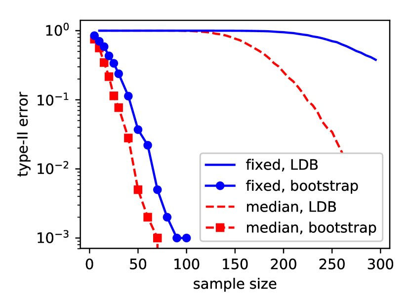
Figure 1: 2D Gaussians with different means.

While there have been various experiments on the type-II error probability, the exponential decay behavior has been scarcely reported. To this end, we perform a simple experiment and display the type-II error probability in the logarithm scale. Let $x^{n}~{}\text{i.i.d.}~{}\sim\mathcal{N}({\mu}_{P},{I})$ and $y^{m}~{}\text{i.i.d.}~{}\sim\mathcal{N}({\mu}_{Q},{I})$, where $\mu_{P}=[0.25,0.25]^{T}$, ${\mu}_{Q}=[1,1]^{T}$, and $I$ is the $2\times 2$ identity matrix. We use the biased test statistic $d_{k}(\hat{P}_{n},\hat{Q}_{m})$ with Gaussian kernel $k(x,y)=\exp(-\|x-y\|_{2}^{2}/w)$. A fixed choice of $w=1$ and the median heuristic are employed for the kernel bandwidth. We also consider two threshold choices: one is from the Large Deviation Bound (LDB), given in Eq. (1); and the other is from a bootstrap method in [15], with $1000$ bootstrap replicates. We repeat $1000$ trials and report the result in Figure 1.

We observe that all the type-II error probabilities exhibit an exponential decay rate as the sample number increases. The LDB threshold is quite conservative and the error probability starts decaying with much more samples. Although the main theorems in Section 3 do not include the median bandwidth, the figure shows that it also leads to an exponential decay of the type-II error probability. This might be because the median distance lies within a small neighborhood of some fixed bandwidth in this experiment, hence behaving similarly.

Kernel choice vs. Sample size

Following the discussions in Section 3.4, we investigate how kernel choice and sample number affect the test performance. We consider Gaussian kernels that are determined by their bandwidths. Sutherland et al. [31] use part of samples as training data to select the bandwidth, which we call the trained bandwidth. The estimated MMD is then computed using the trained bandwidth and the remaining samples.

For the first experiment, we take a similar setting from [31]: $P$ is a $3\times 3$ grid of 2D standard normals, with spacing $10$ between the centers; $Q$ is laid out identically, but with covariance $\frac{\epsilon-1}{\epsilon+1}$ between the coordinates. Here we pick $\epsilon=6$ and generate $n=m=720$ samples from each distribution. We pick splitting ratios $r=0.25$ and $r=0.5$ for computing the trained bandwidth. Correspondingly, there are $n=m=540$ and $n=m=360$ samples used to calculate the test statistic, respectively. For each case with $n=m\in\{360,540,720\}$, we report in Figure 2 the type-II error probabilities over different bandwidths, averaged over $200$ trials. The unbiased test statistic $d_{u}^{2}(\hat{P}_{n},\hat{Q}_{m})$ is used and the test threshold is obtained using bootstrap with $500$ permutations. We also mark the trained bandwidths corresponding to the respective sample sizes in the figure (red star marker).

Figure 2 verifies that the trained bandwidth is close to the optimal one in terms of the type-II error probability. Moreover, it indicates that a large range of bandwidths lead to lower or comparable error probabilities if we directly use the entire samples for testing. As the sample number increases, the exponential decay term in the type-II error probability becomes dominating and the effect of kernel choice diminishes. However, since the desired range of bandwidths is not known in advance, an interesting question is when we shall split data for kernel selection and what is a proper splitting ratio.

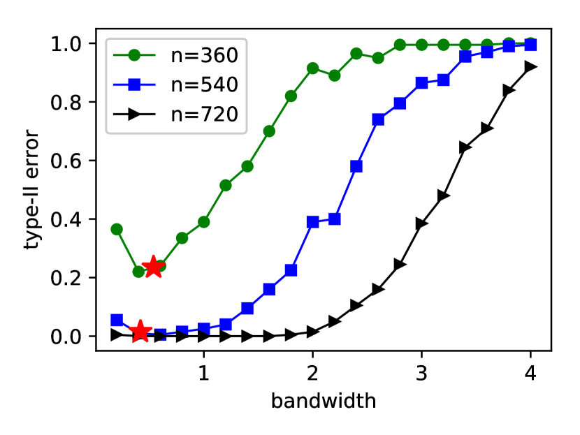
(a)

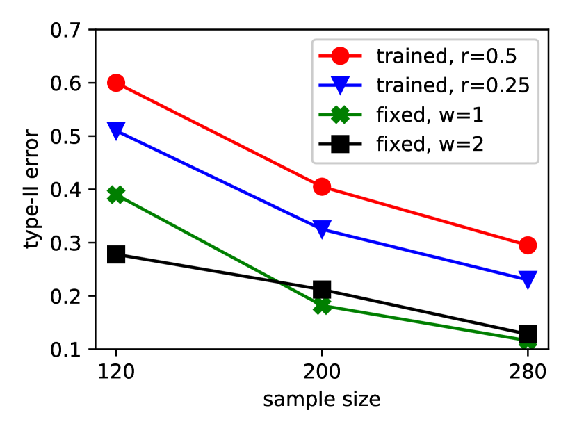
(b)

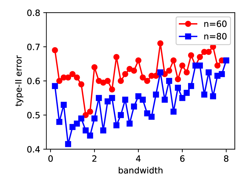
(c)

Figure 2: Kernel choice vs. Sample size. (a) $3\times 3$ grid of 2D standard normals. Red star denotes the trained bandwidth. (b-c) 1D Gaussian mixture.

In the second experiment, we directly use the setup in [23]. We draw $x^{n}~{}\text{i.i.d.}\sim\sum_{k=1}^{5}a_{k}\mathcal{N}(\mu_{k},\sigma^{2})$ with $a_{k}=1/5$, $\sigma^{2}=1$, and $\mu_{k}\sim\operatorname{Uniform}[0,10]$, and then generate $y^{m}$ by adding standard Gaussian noise (perturbation) to $\mu_{k}$. We consider splitting ratios $r=0.25$ and $r=0.5$ of the entire samples used as training data and compute $d_{k}^{2}(\hat{P}_{n},\hat{Q}_{m})$ based on the rest samples. For comparison, the kernel tests with fixed bandwidths $w=1$ and $w=2$ are also evaluated, which estimate the MMD based on the entire samples. All the test thresholds are computed using bootstrap with $500$ replicates. We repeat $500$ trials and report the type-II error probabilities in Figure 2. It shows that the more samples we use to compute the test statistic, the lower type-II error probability we get; in other words, kernel choice is less important than the sample size for this setting. This point is further illustrated in Figure 2 where we show the type-II error probabilities of $n=m=60$ and $n=m=80$ samples over different kernel bandwidths. The kernel selection strategy in [31] does not perform well in this experiment, which also motivates future studies on when to use such a kernel selection strategy.

6 Conclusion

In this paper, a class of kernel two-sample tests are shown to exponentially consistent and to attain the optimal type-II error exponent, provided that kernels are bounded continuous and characteristic. A notable implication is that kernels affect only the sub-exponential term in the type-II error probability. We apply our results to off-line change detection and show that a test achieves the optimal detection in the nonparametric setting. Finally, we empirically investigate how kernel choice and sample size affect the test performance.

Appendix

Appendix A Proof of the extended Sanov’s theorem

We first prove the result with a finite sample space and then extend it to the case with general Polish space. The prerequisites are two combinatorial lemmas that are standard tools in information theory.

For a positive integer $t$, let $\mathcal{P}_{n}(t)$ denote the set of probability distributions defined on $\{1,\ldots,t\}$ of form $P=\left(\frac{n_{1}}{n},\cdots,\frac{n_{t}}{n}\right)$, with integers $n_{1},\ldots,n_{t}$. Stated below are the two lemmas.

Lemma 2 ([7, Theorem 11.1.1]).

$|\mathcal{P}_{n}(t)|\leq(n+1)^{t}.$

Lemma 3 ([7, Theorem 11.1.4]).

Assume $x^{n}$ i.i.d. $\sim Q$ where $Q$ is a distribution defined on $\{1,\ldots,t\}$. For any $P\in\mathcal{P}_{n}(t)$, the probability of the empirical distribution $\hat{P}_{n}$ of $x^{n}$ equal to $P$ satisfies

$$(n+1)^{-t}e^{-nD(P\|Q)}\leq\mathbf{P}_{x^{n}}(\hat{P}_{n}=P)\leq e^{-nD(P\|Q)}.$$

A.1 Finite sample space

Upper bound

Let $t$ denote the cardinality of $\mathcal{X}$. Without loss of generality, assume that $\inf_{(R,S)\in\operatorname{int}\Gamma}cD(R\|P)+(1-c)D(S\|Q)<\infty$. Hence, the open set $\operatorname{int}\Gamma$ is non-empty. As $0<\lim_{n,m\to\infty}\frac{n}{n+m}=c<1$, we can find $n_{0}$ and $m_{0}$ such that there exists $(P^{\prime}_{n},Q^{\prime}_{m})\in\operatorname{int}\Gamma\cap P_{n}(t)\times P_{m}(t)$ for all $n>n_{0}$ and $m>m_{0}$, and that $cD(P_{n}^{\prime}\|P)+(1-c)D(Q_{m}^{\prime}\|Q)\to\inf_{(R,S)\in\operatorname{int}\Gamma}cD(R\|P)+(1-c)D(S\|Q)$ as $n,m\to\infty$. Then we have, with $n>n_{0}$ and $m>m_{0}$,

$$\mathbf{P}_{x^{n}y^{m}}((\hat{P}_{n},\hat{Q}_{m})\in\Gamma) =\sum_{(R,S)\in\Gamma\,\cap\,\mathcal{P}_{n}(t)\times\mathcal{P}_{m}(t)}\mathbf{P}_{x^{n}y^{m}}(\hat{P}_{n}=R,\hat{Q}_{m}=S)$$

$$\geq\sum_{(R,S)\in\operatorname{int}\Gamma\,\cap\,\mathcal{P}_{n}(t)\times\mathcal{P}_{m}(t)}\mathbf{P}_{x^{n}y^{m}}(\hat{P}_{n}=R,\hat{Q}_{m}=S)$$

$$\geq\mathbf{P}_{x^{n}y^{m}}(\hat{P}_{n}=P_{n}^{\prime},\hat{Q}_{m}=Q_{m}^{\prime})$$

$$=\mathbf{P}_{x^{n}}(\hat{P}_{n}=P^{\prime}_{n})\,\mathbf{P}_{y^{m}}(\hat{Q}_{m}=Q^{\prime}_{m})$$

$$\geq(n+1)^{-t}(m+1)^{-t}e^{-nD(P_{n}^{\prime}\|P)}e^{-mD(Q_{m}^{\prime}\|Q)},$$

where the last inequality is from Lemma 3. It follows that

$$~{}~{}~{}~{}\limsup_{n,m\to\infty}-\frac{1}{n+m}\log\mathbf{P}_{x^{n}y^{m}}((\hat{P}_{n},\hat{Q}_{m})\in\Gamma)$$

$$\leq\lim_{n,m\to\infty}\frac{1}{n+m}\left(-t\log((n+1)(m+1))+nD(P^{\prime}_{n}\|P)+mD(Q^{\prime}_{m}\|Q)\right)$$

$$=\lim_{n,m\to\infty}\frac{1}{n+m}\left(nD(P^{\prime}_{n}\|P)+mD(Q^{\prime}_{m}\|Q)\right)$$

$$=\inf_{(R,S)\in\operatorname{int}\Gamma}cD(R\|P)+(1-c)D(S\|Q).$$

Lower bound

$$\mathbf{P}_{x^{n}y^{m}}((\hat{P}_{n},\hat{Q}_{m})\in\Gamma) =\sum_{(R,S)\in\Gamma\cap\mathcal{P}_{n}(t)\times\mathcal{P}_{m}(t)}\mathbf{P}_{x^{n}}(\hat{P}_{n}=R)\,\mathbf{P}_{y^{m}}(\hat{Q}_{m}=S)$$

$$\stackrel{{\scriptstyle(a)}}{{\leq}}\sum_{(R,S)\in\Gamma\cap\mathcal{P}_{n}(t)\times\mathcal{P}_{m}(t)}e^{-nD(R\|P)}e^{-mD(S\|Q)}$$

$$\stackrel{{\scriptstyle(b)}}{{\leq}}(n+1)^{t}(m+1)^{t}\sup_{(R,S)\in\Gamma}e^{-nD(R\|P)}e^{-mD(S\|Q)},$$ (3)

where $(a)$ and $(b)$ are due to Lemma 3 and Lemma 2, respectively. This gives

$$\liminf_{n\to\infty}-\frac{1}{n+m}\log\mathbf{P}_{x^{n}y^{m}}((\hat{P}_{n},\hat{Q}_{m})\in\Gamma)\geq\inf_{(R,S)\in\Gamma}cD(R\|P)+(1-c)D(S\|Q),$$

and hence the lower bound by noting that $\Gamma\in\operatorname{cl}\Gamma$. Indeed, when the right hand side is finite, the infimum over $\Gamma$ equals the infimum over $\operatorname{cl}\Gamma$ as a result of the continuity of KLD for finite alphabets.

A.2 Polish sample space

We consider the general case with $\mathcal{X}$ being a Polish space. Now $\mathcal{P}$ is the space of probability measures on $\mathcal{X}$ endowed with the topology of weak convergence. To proceed, we introduce another topology on $\mathcal{P}$ and an equivalent definition of the KLD.

$\tau$-topology: denote by $\Pi$ the set of all partitions $\mathcal{A}=\{A_{1},\ldots,A_{t}\}$ of $\mathcal{X}$ into a finite number of measurable sets $A_{i}$. For $P\in\mathcal{P}$, $\mathcal{A}\in\Pi$, and $\zeta>0$, denote

$$U(P,\mathcal{A},\zeta)=\{P^{\prime}\in\mathcal{P}:|P^{\prime}(A_{i})-P(A_{i})|<\zeta,i=1,\dots,t\}.$$ (4)

The $\tau$-topology on $\mathcal{P}$ is the coarsest topology in which the mapping $P\to P(F)$ are continuous for every measurable set $F\subset\mathcal{X}$. A base for this topology is the collection of the sets (4). We will use $\mathcal{P}_{\tau}$ when we refer to $\mathcal{P}$ endowed with this $\tau$-topology, and write the interior and closure of a set $\Gamma\in\mathcal{P}_{\tau}$ as $\operatorname{int}_{\tau}\Gamma$ and $\operatorname{cl}_{\tau}\Gamma$, respectively. We remark that the $\tau$-topology is stronger than the weak topology: any open set in $\mathcal{P}$ w.r.t. weak topology is also open in $\mathcal{P}_{\tau}$ (see more details in [8, 9]). The product topology on $\mathcal{P}_{\tau}\times\mathcal{P}_{\tau}$ is determined by the base of the form of

$$U(P,\mathcal{A}_{1},\zeta_{1})\times U(Q,\mathcal{A}_{2},\zeta_{2}),$$

for $(P,Q)\in\mathcal{P}_{\tau}\times\mathcal{P}_{\tau}$, $\mathcal{A}_{1},\mathcal{A}_{2}\in\Pi$, and $\zeta_{1},\zeta_{2}>0$. We still use $\operatorname{int}_{\tau}(\Gamma)$ and $\operatorname{cl}_{\tau}(\Gamma)$ to denote the interior and closure of a set $\Gamma\subset\mathcal{P}_{\tau}\times\mathcal{P}_{\tau}$. As there always exists $\mathcal{A}\in\Pi$ that refines both $\mathcal{A}_{1}$ and $\mathcal{A}_{2}$, any element from the base has an open subset

$$\tilde{U}(P,Q,\mathcal{A},\zeta):=U(P,\mathcal{A},\zeta)\times U(Q,\mathcal{A},\zeta)\subset\mathcal{P}_{\tau}\times\mathcal{P}_{\tau},$$

for some $\zeta>0$.

Another definition of the KLD: an equivalent definition of the KLD will also be used:

$$D(P\|Q)=\sup_{\mathcal{A}\in\Pi}\sum_{i=1}^{t}P(A_{i})\log\frac{P(A_{i})}{Q(A_{i})}=\sup_{\mathcal{A}\in\Pi}D(P^{\mathcal{A}}\|Q^{\mathcal{A}}),$$

with the conventions $0\log 0=0\log\frac{0}{0}=0$ and $a\log\frac{a}{0}=+\infty$ if $a>0$. Here $P^{\mathcal{A}}$ denotes the discrete probability measure $(P(A_{1}),\ldots,P(A_{t}))$ obtained from probability measure $P$ and partition $\mathcal{A}$. It is not hard to verify that for $0<c<1$,

$$cD(R\|P)+(1-c)D(S\|Q) =c\sup_{\mathcal{A}_{1}\in\Pi}D(R^{\mathcal{A}_{1}}\|P^{\mathcal{A}_{1}})+(1-c)\sup_{\mathcal{A}_{2}\in\Pi}D(S^{\mathcal{A}_{2}}\|Q^{\mathcal{A}_{2}})$$

$$=\sup_{\mathcal{A}\in\Pi}\left(cD\left(R^{\mathcal{A}}\|P^{\mathcal{A}}\right)+(1-c)D\left(S^{\mathcal{A}}\|Q^{\mathcal{A}}\right)\right),$$ (5)

due to the existence of $\mathcal{A}$ that refines both $\mathcal{A}_{1}$ and $\mathcal{A}_{2}$ and the log-sum inequality [7].

We are ready to show the extended Sanov’s theorem with Polish space.

Upper bound

It suffices to consider only non-empty open $\Gamma$. If $\Gamma$ is open in $\mathcal{P}\times\mathcal{P}$, then $\Gamma$ is also open in $\mathcal{P}_{\tau}\times\mathcal{P}_{\tau}$. Therefore, for any $(R,S)\in\Gamma$, there exists a finite (measurable) partition $\mathcal{A}=\{A_{1},\ldots,A_{t}\}$ of $\mathcal{X}$ and $\zeta>0$ such that

$$\tilde{U}(R,S,\mathcal{A},\zeta)=\left\{(R^{\prime},S^{\prime}):|R(A_{i})-R^{\prime}(A_{i})|<\zeta,|S(A_{i})-S^{\prime}(A_{i})|<\zeta,i=1,\ldots,t\right\}\subset\Gamma.$$ (6)

Define the function $T:\mathcal{X}\to\{1,\ldots,t\}$ with $T(x)=i$ for $x\in A_{i}$. Then $(\hat{P}_{n},\hat{Q}_{m})\in\tilde{U}(R,S,\mathcal{A},\zeta)$ with $R,S\in\Gamma$ if and only if the empirical measures $\hat{P}^{\circ}_{n}$ of $\{T(x_{1}),\ldots,T(x_{n})\}:=T(x^{n})$ and $\hat{Q}^{\circ}_{m}$ of $\{T(y_{1}),\ldots,T(y_{m})\}:=T(y^{m})$ lie in

$$U^{\circ}(R,S,\mathcal{A},\zeta)=\{(R^{\circ},S^{\circ}):|R^{\circ}(i)-R(A_{i})|<\zeta,|S^{\circ}(i)-S(A_{i})|<\zeta,i=1,\ldots,t\}\subset\mathbb{R}^{t}\times\mathbb{R}^{t}.$$

Thus, we have

$$\mathbf{P}_{x^{n}y^{m}}((\hat{P}_{n},\hat{Q}_{m})\in\Gamma) \geq\mathbf{P}_{x^{n}y^{m}}((\hat{P}_{n},\hat{Q}_{m})\in\tilde{U}(R,S,\mathcal{A},\zeta))$$

$$=\mathbf{P}_{T(x^{n})T(y^{m})}((\hat{P}_{n}^{\circ},\hat{Q}_{m}^{\circ})\in U^{\circ}(R,S,\mathcal{A},\zeta)).$$

As $T(x)$ and $T(y)$ takes values from a finite alphabet and $U^{\circ}(R,S,\mathcal{A},\zeta)$ is open, we obtain that

$$~{}\limsup_{n\to\infty}-\frac{1}{n+m}\log\mathbf{P}_{x^{n}y^{m}}((\hat{P}_{n},\hat{Q}_{m})\in\Gamma)$$

$$\leq ~{}\limsup_{n\to\infty}-\frac{1}{n+m}\log\mathbf{P}_{T(x^{n})T(y^{m})}((\hat{P}_{n}^{\circ},\hat{Q}_{m}^{\circ})\in U^{\circ}(R,S,\mathcal{A},\zeta))$$

$$\leq ~{}\inf_{(R^{\circ},S^{\circ})\in U^{\circ}(R,S,\mathcal{A},\zeta)}cD(R^{\circ}\|P^{\mathcal{A}})+(1-c)D(S^{\circ}\|Q^{\mathcal{A}})$$

$$= ~{}\inf_{(R^{\prime},S^{\prime})\in\tilde{U}(R,S,\mathcal{A},\zeta)}cD(R^{\prime\mathcal{A}}\|P^{\mathcal{A}})+(1-c)D(S^{\prime\mathcal{A}}\|Q^{\mathcal{A}})$$

$$\leq ~{}cD(R\|P)+(1-c)D(S\|Q),$$ (7)

where we have used definition of KLD in Eq. (A.2) and $(R,S)\in\tilde{U}(R,S,\mathcal{A},\zeta)$ in the last inequality. As $(R,S)$ is arbitrary in $\Gamma$, the lower bound is established by taking infimum over $\Gamma$.

Lower bound

With notations

$$\Gamma^{\mathcal{A}}=\{(R^{\mathcal{A}},S^{\mathcal{A}}):(R,S)\in\Gamma\},~{}\Gamma(\mathcal{A})=\{(R,S):(R^{\mathcal{A}},S^{\mathcal{A}})\in\Gamma^{\mathcal{A}}\},$$

where $\mathcal{A}=\{A_{1},\ldots,A_{t}\}$ is a finite partition, it holds that

$$~{}\mathbf{P}_{x^{n}y^{m}}((\hat{P}_{n},\hat{Q}_{m})\in\Gamma)$$

$$\leq ~{}\mathbf{P}_{x^{n}y^{m}}((\hat{P}_{n},\hat{Q}_{m})\in\Gamma({\mathcal{A}}))$$

$$= ~{}\mathbf{P}_{x^{n}y^{m}}((\hat{P}_{n}^{\mathcal{A}},\hat{Q}_{m}^{\mathcal{A}})\in\Gamma^{\mathcal{A}}\cap\mathcal{P}_{n}(t)\times{\mathcal{P}_{m}}(t))$$

$$\leq ~{}(n+1)^{t}(m+1)^{t}\max_{(R^{\circ},S^{\circ})\in\Gamma^{\mathcal{A}}\cap\mathcal{P}_{n}(t)\times{\mathcal{P}_{m}(t)}}\mathbf{P}_{x^{n}y^{m}}\left(\hat{P}_{n}=R^{\circ},\hat{Q}_{m}=S^{\circ}\right)$$

$$\leq ~{}(n+1)^{t}(m+1)^{t}\exp\left(-\inf_{(R,S)\in\Gamma}\left(nD(R^{\mathcal{A}}\|P^{\mathcal{A}})+mD(S^{\mathcal{A}}\|Q^{\mathcal{A}})\right)\right),$$

where the last two inequalities are from Lemmas 2 and 3. As the above holds for any $\mathcal{A}\in\Pi$, Eq. (A.2) indicates

$$~{}\limsup_{n\to\infty}\frac{1}{n+m}\log\mathbf{P}_{x^{n}y^{m}}((\hat{P}_{n},\hat{Q}_{m})\in\Gamma)$$

$$\leq ~{}\inf_{\mathcal{A}}\left(-\inf_{(R,S)\in\Gamma}\left(cD(R^{\mathcal{A}}\|P^{\mathcal{A}})+(1-c)D(S^{\mathcal{A}}\|Q^{\mathcal{A}})\right)\right)$$

$$= ~{}-\sup_{\mathcal{A}}\inf_{(R,S)\in\Gamma}cD(R^{\mathcal{A}}\|P^{\mathcal{A}})+(1-c)D(S^{\mathcal{A}}\|Q^{\mathcal{A}}).$$

Then the remaining of obtaining the lower bound is to show

$$\sup_{\mathcal{A}}\inf_{(R,S)\in\Gamma}cD(R^{\mathcal{A}}\|P^{\mathcal{A}})+(1-c)D(S^{\mathcal{A}}\|Q^{\mathcal{A}})\geq\inf_{(R,S)\in\operatorname{cl}\Gamma}cD(R\|P)+(1-c)D(S\|Q).$$

Assuming, without loss of generality, that the left hand side is finite, we only need to show

$$\operatorname{cl}\Gamma\cap B(P,Q,\eta)\neq\varnothing,$$

whenever

$$\eta>\sup_{\mathcal{A}}\inf_{(R,S)\in\Gamma}cD(R^{\mathcal{A}}\|P^{\mathcal{A}})+(1-c)D(S^{\mathcal{A}}\|Q^{\mathcal{A}}).$$

Here $B(P,Q,\eta)$ is the divergence ball defined as follows

$$B(P,Q,\eta)=\left\{(R,S):cD(R\|P)+(1-c)D(S\|Q)\leq\eta\right\},$$

which is compact in $\mathcal{P}\times\mathcal{P}$ w.r.t. the weak topology, due to the lower semi-continuity of $D(\cdot\|P)$ and $D(\cdot\|Q)$ as well as the fact that $0<c<1$.

To this end, we first show the following:

$$\operatorname{cl}\Gamma=\bigcap_{\mathcal{A}}\operatorname{cl}\Gamma(\mathcal{A}).$$ (8)

The inclusion is obvious since $\Gamma\in\Gamma(\mathcal{A})$. The reverse means that if $(R,S)\in\operatorname{cl}\Gamma(\mathcal{A})$ for each $\mathcal{A}$, then any neighborhood of $(R,S)$ w.r.t. the weak convergence intersects $\Gamma$. To verify this, let $O(R,S)$ be a neighborhood of $(R,S)$ w.r.t. the weak convergence, then there exists $\tilde{U}(R,S,\mathcal{B},\zeta)\in O(R,S)$ over a finite partition $\mathcal{B}$ as $O(R,S)$ is also open in $\mathcal{P}_{\tau}\times\mathcal{P}_{\tau}$. Furthermore, the partition $\mathcal{B}$ can be chosen to refine $\mathcal{A}$ so that $\operatorname{cl}\Gamma(\mathcal{B})\subset\operatorname{cl}\Gamma(\mathcal{A})$. As $\tau$-topology is stronger than the weak topology, a closed set in the $\mathcal{P}_{\tau}\times\mathcal{P}_{\tau}$ is closed in $\mathcal{P}\times\mathcal{P}$, and hence $\operatorname{cl}\Gamma(\mathcal{B})\subset\operatorname{cl}_{\tau}\Gamma(\mathcal{B})$. That $(R,S)\in\operatorname{cl}_{\tau}\Gamma(\mathcal{B})$ implies that there exists $(R^{\prime},S^{\prime})\in\tilde{U}(R,S,\mathcal{B},\zeta)\cap\Gamma(\mathcal{B})$. By the definition of $\Gamma(\mathcal{B})$, we can also find $(\tilde{R},\tilde{S})\in\Gamma$ such that $\tilde{R}(B_{i})=R^{\prime}(B_{i})$ and $\tilde{S}(B_{i})=S^{\prime}(B_{i})$ for each $B_{i}\in\mathcal{B}$, and hence $(\tilde{R},\tilde{S})\in\tilde{U}(R,S,\mathcal{B},\zeta)$. In summary, we have $(\tilde{R},\tilde{S})\in\tilde{U}(R,S,\mathcal{B},\zeta)\subset O(R,S)$ and $(\tilde{R},\tilde{S})\in\Gamma$. Therefore, $\Gamma\cap O(R,S)\neq\varnothing$ and the claim follows.

Next we show that, for each partition $\mathcal{A}$,

$$\Gamma(\mathcal{A})\cap B(P,Q,\eta)\neq\varnothing.$$ (9)

By Eq. (A.2), there exists $(\tilde{P},\tilde{Q})$ such that $cD(\tilde{P}^{\mathcal{A}}\|P^{\mathcal{A}})+(1-c)D(\tilde{Q}^{\mathcal{A}}\|Q^{\mathcal{A}})\leq\eta$. For such $(\tilde{P},\tilde{Q})$, we can construct $(P^{\prime},Q^{\prime})\in\Gamma(\mathcal{A})$ as

$$P^{\prime}(F) =\sum_{i=1}^{t}\frac{\tilde{P}(A_{i})}{P(A_{i})}P(F\cap A_{i}),$$

$$Q^{\prime}(F) =\sum_{i=1}^{t}\frac{\tilde{Q}(A_{i})}{Q(A_{i})}Q(F\cap A_{i}),$$

for any measurable subset $F\subset\mathcal{X}$. If $P(A_{i})=0$ ($Q(A_{i})=0$) and hence $\tilde{P}(A_{i})=0$ ($\tilde{Q}(A_{i})=0$), as $D(\tilde{P}^{\mathcal{A}}\|P^{\mathcal{A}})<\infty$ ($D(\tilde{Q}^{\mathcal{A}}\|Q^{\mathcal{A}})<\infty$), for some $i$, the corresponding term in the above equation is set equal to $0$. Then $(P^{\prime},Q^{\prime})$ belongs to $\Gamma(\mathcal{A})$ and also lies in $B(P,Q,\eta)$. The latter is because $D(P^{\prime}\|P)=D(\tilde{P}^{\mathcal{A}}\|Q^{\mathcal{A}})$ and $D(Q^{\prime}\|Q)=D(\tilde{Q}^{\mathcal{A}}\|Q^{\mathcal{A}})$: one can verify that any $\mathcal{B}$ that refines $\mathcal{A}$ satisfies

$$D({P}^{\prime\mathcal{B}}\|P^{\mathcal{B}})=D(\tilde{P}^{\mathcal{A}}\|P^{\mathcal{A}}),D({Q}^{\prime\mathcal{B}}\|Q^{\mathcal{B}})=D(\tilde{Q}^{\mathcal{A}}\|Q^{\mathcal{A}}).$$

For any finite collection of partitions $\mathcal{A}_{i}\in\Pi$ and $\mathcal{A}\in\Pi$ refining each $\mathcal{A}_{i}$, each $\Gamma(\mathcal{A}_{i})$ contains $\Gamma(\mathcal{A})$. This implies that

$$\bigcap_{i=1}^{r}\left(\Gamma(\mathcal{A}_{i})\cap B(p,q,\eta)\right)\neq\varnothing,$$

for any finite $r$. Finally, the set $\operatorname{cl}\Gamma(\mathcal{A})\cap B(P,Q,\eta)$ for any $\mathcal{A}$ is compact due to the compactness of $B(P,Q,\eta)$, and any finite collection of them has non-empty intersection. It follows that all these sets is also non-empty. This completes the proof.

Appendix B Proof of Theorem 3

Two lemmas are needed: the first states the optimal type-II error exponent of any level $\alpha$ test for simple hypothesis testing between two known distributions $P$ and $Q$, and the second provides a large deviation bound on $d_{k}(P,\hat{P}_{n})$.

Lemma 4 (Stein’s lemma [7, 9]).

Let $x^{n}$ i.i.d. $\sim R$. Consider the test between $H_{0}:R=P$ and $H_{1}:R=Q$ with $0<D(P\|Q)<\infty$. Given $0<\alpha<1$, let $\Omega^{*}(n)=(\Omega_{0}^{*}(n),\Omega_{1}^{*}(n))$ be the optimal level $\alpha$ test such that the type-II error probability is minimized. Then the type-II error probability decreases exponentially at a rate of $D(P\|Q)$ as $n\to\infty$, that is,

$$\lim_{n\to\infty}-\frac{1}{n}\log Q(\Omega_{0}^{*}(n))=D(P\|Q).$$

Lemma 5 ([32, 33]).

Let $P$, $x^{n}$, and $\hat{P}_{n}$ be defined as in Section 2. Let $k$ be bounded continuous and characteristic, with $0\leq k(\cdot,\cdot)\leq K$. When $x^{n}~{}\text{i.i.d.}\sim P$,

$$\mathbf{P}_{x^{n}}\left(d_{k}(P,\hat{P}_{n})>\left({2K}/{n}\right)^{1/2}+\epsilon\right)\leq\exp{\left(-\frac{\epsilon^{2}n}{2K}\right)}.$$

Proof.

According to Theorem 1, $d_{k}$ metrizes the weak convergence over $\mathcal{P}$. That $\alpha_{n,m}\leq\alpha$ is clear from Lemma 1, and we only need to show that $\beta_{n,m}$ vanishes exponentially as $n$ and $m$ scale. For convenience, we will write the error exponent of $\beta_{n,m}$ as $\beta$.

We first show $\beta\geq D^{*}$. With a fixed $\gamma>0$, we have $\gamma_{n,m}\leq\gamma$ for sufficiently large $n$ and $m$. Therefore,

$$\beta =\liminf_{n,m\to\infty}-\frac{1}{n+m}\log\mathbf{P}_{x^{n}y^{m}}(d_{k}(\hat{P}_{n},\hat{Q}_{m})\leq\gamma_{n,m})$$

$$\geq\liminf_{n,m\to\infty}-\frac{1}{n+m}\log\mathbf{P}_{x^{n}y^{m}}(d_{k}(\hat{P}_{n},\hat{Q}_{m})\leq\gamma)$$

$$\geq\inf_{(R,S):d_{k}(R,S)\leq\gamma}cD(R\|P)+(1-c)D(S\|Q)$$

$$:=D_{\gamma}^{*},$$ (10)

where the last inequality is from the extended Sanov’s theorem and that $d_{k}$ metrizes weak convergence of $\mathcal{P}$ so that $\{(R,S):d_{k}(R,S)\leq\gamma\}$ is closed in the product topology on $\mathcal{P}\times\mathcal{P}$. Since $\gamma>0$ can be arbitrarily small, we have

$$\beta\geq\lim_{\gamma\to 0^{+}}D^{*}_{\gamma},$$

where the limit on the right hand side must exist as $D^{*}_{\gamma}$ is positive, non-decreasing when $\gamma$ decreases, and bounded by $D^{*}$ that is assumed to be finite. Then it suffices to show

$$\lim_{\gamma\to 0^{+}}D_{\gamma}^{*}=D^{*}.$$

To this end, let $(R_{\gamma},S_{\gamma})$ be such that $d_{k}(R_{\gamma},S_{\gamma})\leq\gamma$ and $cD(R_{\gamma}\|P)+(1-c)D(S_{\gamma}\|Q)=D^{*}_{\gamma}$. Notice that $R_{\gamma}$ and $S_{\gamma}$ must lie in

$$\left\{W:D(W\|P)\leq\frac{D^{*}}{c},D(W\|Q)\leq\frac{D^{*}}{1-c}\right\}:=\mathcal{W},$$

for otherwise $D_{\gamma}^{*}>D^{*}$. We remark that $\mathcal{W}$ is a compact set in $\mathcal{P}$ as a result of the lower semi-continuity of KLD w.r.t. the weak topology on $\mathcal{P}$ [34, 9]. Existence of such a pair can be seen from the facts that $\{(R,S):d_{k}(R,S)\leq\gamma\}$ is closed and convex, and that both $D(\cdot{\|P})$ and $D(\cdot\|Q)$ are convex functions [34].

Assume that $D^{*}$ cannot be achieved. We can write

$$\lim_{\gamma\to 0^{+}}D^{*}_{\gamma}=D^{*}-\epsilon,$$ (11)

for some $\epsilon>0$. By the definition of lower semi-continuity, there exists a $\kappa_{W}>0$ for each $W\in\mathcal{W}$ such that

$$cD(R\|P)+(1-c)D(S\|Q)\geq cD(W\|P)+(1-c)D(W\|Q)-\frac{\epsilon}{2}\geq D^{*}-\frac{\epsilon}{2},$$ (12)

whenever $R$ and $S$ are both from

$$\mathcal{S}_{W}=\left\{R:d_{k}(R,W)<\kappa_{W}\right\}.$$

Here the last inequality comes from the definition of $D^{*}$ given in Theorem 3. To find a contradiction, define

$$\mathcal{S}_{W}^{\prime}=\left\{R:d_{k}(R,W)<\frac{\kappa_{W}}{2}\right\}.$$

Since $S_{W}^{\prime}$ is open and $\bigcup_{W}\mathcal{S}_{W}^{\prime}$ covers $\mathcal{W}$, the compactness of $\mathcal{W}$ implies that there exists finite $\mathcal{S}_{W}^{\prime}$’s, denoted by $\mathcal{S}_{W_{1}}^{\prime},\ldots,\mathcal{S}_{W_{N}}^{\prime}$, covering $\mathcal{W}$. Define $\kappa^{*}=\min_{i=1}^{N}\kappa_{W_{i}}>0$. Now let $\gamma<{\kappa^{*}}/{2}$ as $\gamma$ can be made arbitrarily small. Since $\bigcup_{i=1}^{N}\mathcal{S}^{\prime}_{W_{i}}$ covers $\mathcal{W}$, we can find a $W_{i}$ with $R_{\gamma}\in\mathcal{S}_{W_{i}}^{\prime}\subset\mathcal{S}_{W_{i}}$. Thus, it holds that

$$d_{k}(S_{\gamma},W_{i})\leq d_{k}(S_{\gamma},R_{\gamma})+d_{k}(R_{\gamma},W_{i})<\kappa_{W_{i}}.$$

That is, $S_{\gamma}$ also lies in $\mathcal{S}_{W_{i}}$. By Eq. (12) we get

$$cD(R_{\gamma}\|P)+(1-c)D(S_{\gamma}\|Q)\geq D^{*}-\epsilon/2.$$

However, by our assumption in Eq. (11), it should hold that

$$cD(R_{\gamma}\|P)+(1-c)D(S_{\gamma}\|Q)\leq D^{*}-\epsilon.$$

Therefore, $\beta\geq D^{*}$.

The other direction can be simply seen from the optimal type-II error exponent in Theorem 5. Alternatively, we can use Stein’s lemma in a similar manner to the proof of [36, Theorem 4]. Let $P^{\prime}$ be such that $cD(P^{\prime}\|P)+(1-c)D(P^{\prime}\|Q)=D^{*}.$ Such $P^{\prime}$ exists because $0<D^{*}<\infty$ and $D(\cdot\|P)$ and $D(\cdot\|Q)$ are convex w.r.t. $\mathcal{P}$. That $D^{*}$ is bounded implies that both $D(P^{\prime}\|P)$ and $D(P^{\prime}\|Q)$ are finite. We have

$$\beta_{n,m}= ~{}\mathbf{P}_{x^{n}y^{m}}(d_{k}(\hat{P}_{n},\hat{Q}_{m})\leq\gamma_{n,m})$$

$$\stackrel{{\scriptstyle(a)}}{{\geq}} ~{}\mathbf{P}_{x^{n}y^{m}}(d_{k}(\hat{P}_{n},P^{\prime})+d_{k}(\hat{Q}_{m},P^{\prime})\leq{\gamma_{n,m}})$$

$$\stackrel{{\scriptstyle(b)}}{{\geq}} ~{}\mathbf{P}_{x^{n}y^{m}}(d_{k}(\hat{P}_{n},P^{\prime})\leq\gamma_{n},d_{k}(\hat{Q}_{m},P^{\prime})\leq{\gamma_{m}})$$

$$= ~{}P(d_{k}(\hat{P}_{n},P^{\prime})\leq\gamma_{n})\,Q(d_{k}(\hat{Q}_{m},P^{\prime})\leq{\gamma_{m}}),$$

where $(a)$ and $(b)$ are from the triangle inequality of the metric $d_{k}$, and we pick $\gamma_{n}=\sqrt{2K/n}(1+\sqrt{-\log\alpha})$, and $\gamma_{m}=\sqrt{2K/m}(1+\sqrt{-\log\alpha})$ so that $\gamma_{n,m}>\gamma_{n}+\gamma_{m}$. Then Lemma 5 implies $P^{\prime}(d_{k}(\hat{P}_{n},P^{\prime})\leq\gamma_{n})>1-\alpha$. For now assume that $D(P^{\prime}\|P)>0$ and $D(P^{\prime}\|Q)>0$. We can regard $\{x^{n}:d_{k}(\hat{P}_{n},P^{\prime})\leq\gamma_{n}\}$ as an acceptance region for testing $H_{0}:x^{n}\sim P^{\prime}$ and $H_{1}:x^{n}\sim P$. Clearly, this test performs no better than the optimal level $\alpha$ test for this simple hypothesis testing in terms of the type-II error probability. Therefore, Stein’s lemma implies

$$\liminf_{n\to\infty}-\frac{1}{n}\log P(d_{k}(\hat{P}_{n},P^{\prime})\leq\gamma_{n})\leq D(P^{\prime}\|P).$$ (13)

Analogously, we have

$$\liminf_{m\to\infty}-\frac{1}{m}\log Q(d_{k}(\hat{Q}_{m},P^{\prime})\leq\gamma_{m})\leq D(P^{\prime}\|Q).$$ (14)

Now assume without loss of generality that $D(P^{\prime}\|P)=0$, i.e., $P^{\prime}=P$. Then $D(P^{\prime}\|Q)>0$ under the alternative hypothesis $H_{1}:P\neq Q$, and Eq. (14) still holds. Using Lemma 5, we have $P(d_{k}(\hat{P}_{n},P^{\prime})\leq\gamma_{n})>1-\alpha$, which gives zero exponent. Therefore, Eq. (13) holds with $P^{\prime}=P$.

As $\lim_{n,m\to\infty}\frac{n}{n+m}=c$, we conclude that

$$\beta=\liminf_{n,m\to\infty}-\frac{1}{n+m}\log\beta_{n,m}\leq D^{*}.$$

The proof is complete. ∎

Appendix C Proof of Theorem 4

Proof.

Let $P^{\prime}$ be such that $cD(P^{\prime}\|P)+(1-c)D(P^{\prime}\|Q)=D^{*}$. Consider first $D(P^{\prime}\|P)\neq 0$ and $D(P^{\prime}\|Q)\neq 0$. Since $D^{*}$ is assumed to be finite, we have both $D(P^{\prime}\|P)$ and $D(P^{\prime}\|Q)$ being finite. This implies that $P^{\prime}$ is absolutely continuous with respect to both $P$ and $Q$, so the Radon-Nikodym derivatives ${dP^{\prime}}/{dP}$ and ${dP^{\prime}}/{dQ}$ exist.

Define two sets

$$A_{n} =\left\{x^{n}:D(P^{\prime}\|P)-\epsilon\leq\frac{1}{n}\log\frac{dP^{\prime}(x^{n})}{dP(x^{n})}\leq D(P^{\prime}\|P)+\epsilon\right\},$$ (15)

$$B_{m} =\left\{y^{m}:D(P^{\prime}\|Q)-\epsilon\leq\frac{1}{m}\log\frac{dP^{\prime}(y^{m})}{dQ(y^{m})}\leq D(P^{\prime}\|Q)+\epsilon\right\},$$

Recall the definition of the KLD: $D(P^{\prime}\|P)=\mathbf{E}_{x\sim P^{\prime}}\log(dP^{\prime}(x)/dP(x))$ and $D(P^{\prime}\|Q)=\mathbf{E}_{x\sim P^{\prime}}\log(dP^{\prime}(x)/dQ(x))$. By law of large numbers, we have for any given $\epsilon>0$,

$$\mathbf{P}_{x^{n}y^{m}}(A_{n}\times B_{m})\geq 1-\epsilon,~{}\text{for large enough}~{}n~{}\text{and}~{}m,$$ (16)

with $x^{n}$ and $y^{m}$ i.i.d. $\sim P^{\prime}$.

Now consider the type-II error probability of level $\alpha$ tests. First, for a level $\alpha$ test, we have its acceptance region satisfies

$$\mathbf{P}_{x^{n}y^{m}}(\mbox{${\cal A}$}^{\prime}(n,m))>1-\alpha,$$ (17)

when $x^{n}$ and $y^{m}$ i.i.d. $\sim P^{\prime}$, i.e., when the null hypothesis $H_{0}:P=Q$ holds. Then under the alternative hypothesis $H_{1}:P\neq Q$, we have

$$\beta^{\prime}_{n,m} =\mathbf{P}_{x^{n}y^{m}}(\mathcal{A}^{\prime}_{0}(n,m))$$

$$\geq\mathbf{P}_{x^{n}y^{m}}(A_{n}\times B_{m}\cap\mathcal{A}^{\prime}(n,m))$$

$$=\int_{A_{n}\times B_{m}\cap\mathcal{A}^{\prime}(n,m)}dP(x^{n})\,dQ(y^{m})$$

$$\stackrel{{\scriptstyle(a)}}{{\geq}}\int_{A_{n}\times B_{m}\cap\mathcal{A}^{\prime}(n,m)}2^{-n(D(P^{\prime}\|P)+\epsilon)}2^{-m(D(P^{\prime}\|Q)+\epsilon)}dP^{\prime}(x^{n})\,dP^{\prime}(y^{m})$$

$$=2^{-nD(P^{\prime}\|P)-m(D(P^{\prime}\|Q)-(n+m)\epsilon}\int_{A_{n}\times B_{m}\cap\mathcal{A}^{\prime}(n,m)}dP^{\prime}(x^{n})\,dP^{\prime}(y^{m})$$

$$\stackrel{{\scriptstyle(b)}}{{\geq}}2^{-nD(P^{\prime}\|P)-mD(P^{\prime}\|Q)-(n+m)\epsilon}(1-\alpha-\epsilon),$$

where $(a)$ is from Eq. (15) and $(b)$ is due to Eqs. (16) and (17). Thus, when $\epsilon$ is small enough so that $1-\alpha-\epsilon>0$, we get

$$\liminf_{n,m\to\infty}-\frac{1}{n+m}\log\beta^{\prime}_{n,m} \leq\liminf_{n,m\to\infty}\frac{1}{n+m}\left(nD(P^{\prime}\|P)+m(D(P^{\prime}\|Q)+(n+m)\epsilon\right)$$

$$=D^{*}+\epsilon.$$ (18)

If a test is an asymptotic level $\alpha$ test, we can replace $\alpha$ by $\alpha+\epsilon^{\prime}$ where $\epsilon^{\prime}$ can be made arbitrarily small provided that $n$ and $m$ are large enough. Thus, Eq. (C) holds too. Finally, since $\epsilon$ can also be arbitrarily small, we conclude that

$$\lim_{n,m\to\infty}-\frac{1}{n+m}\log\beta^{\prime}_{n,m}\leq D^{*}.$$

If $P^{\prime}=P$, then $A_{n}$ contains all $x^{n}\in\mathcal{X}^{n}$ and the above procedure gives the same result.

The same argument also applies the case with $\lim_{n,m\to\infty}\frac{n}{m}=\infty$ and we have

$$\lim_{n,m\to\infty}-\frac{1}{m}\log\beta^{\prime}_{n,m}\leq D(P\|Q).$$

∎

References

• Arjovsky et al. [2017] M. Arjovsky, S. Chintala, and L. Bottou. Wasserstein GAN. arXiv preprint arXiv:1701.07875, 2017.
• Basseville and Nikiforov [1993] M. Basseville and I. V. Nikiforov. Detection of Abrupt Changes: Theory and Application. Englewood Cliffs: Prentice Hall, 1993.
• Berlinet and Thomas-Agnan [2011] A. Berlinet and C. Thomas-Agnan. Reproducing Kernel Hilbert Spaces in Probability and Statistics. Springer Science & Business Media, 2011.
• Borgwardt et al. [2006] K. M. Borgwardt, A. Gretton, M. J. Rasch, H.-P. Kriegel, B. Schölkopf, and A. J. Smola. Integrating structured biological data by kernel maximum mean discrepancy. Bioinformatics, 22(14):e49–e57, July 2006.
• Bu et al. [2016] Y. Bu, S. Zou, Y. Liang, and V. V. Veeravalli. Estimation of KL divergence: Optimal minimax rate. arXiv preprint arXiv:1607.02653, 2016.
• Casella and Berger [2002] G. Casella and R. Berger. Statistical Inference. Duxbury Thomson Learning, 2002.
• Cover and Thomas [2006] T. M. Cover and J. A. Thomas. Elements of Information Theory. New York: Wiley, 2nd edition, 2006.
• Csiszár [2006] I. Csiszár. A simple proof of Sanov’s theorem. Bulletin of the Brazilian Mathematical Society, 37(4):453–459, 2006.
• Dembo and Zeitouni [2009] A. Dembo and O. Zeitouni. Large Deviations Techniques and Applications. New York: Springer, 2009.
• Desobry et al. [2005] F. Desobry, M. Davy, and C. Doncarli. An online kernel change detection algorithm. IEEE Transactions on Signal Processing, 53(8):2961–2974, 2005.
• Dziugaite et al. [2015] G. K. Dziugaite, D. M. Roy, and Z. Ghahramani. Training generative neural networks via maximum mean discrepancy optimization. In Proceedings of the Thirty-First Conference on Uncertainty in Artificial Intelligence, 2015.
• Friedman and Rafsky [1979] J. H. Friedman and L. C. Rafsky. Multivariate generalizations of the Wald-Wolfowitz and Smirnov two-sample tests. The Annals of Statistics, pages 697–717, 1979.
• Fukumizu et al. [2009] K. Fukumizu, A. Gretton, G. R. Lanckriet, B. Schölkopf, and B. K. Sriperumbudur. Kernel choice and classifiability for RKHS embeddings of probability distributions. In Advances in Neural Information Processing Systems, 2009.
• Gretton et al. [2009] A. Gretton, K. Fukumizu, Z. Harchaoui, and B. Sriperumbudur. A fast, consistent kernel two-sample test. In Advances in Neural Information Processing Systems, 2009.
• Gretton et al. [2012a] A. Gretton, K. M. Borgwardt, M. J. Rasch, B. Schölkopf, and A. Smola. A kernel two-sample test. Journal of Machine Learning Research, 13(Mar):723–773, 2012a.
• Gretton et al. [2012b] A. Gretton, D. Sejdinovic, H. Strathmann, S. Balakrishnan, M. Pontil, K. Fukumizu, and B. K. Sriperumbudur. Optimal kernel choice for large-scale two-sample tests. In Advances in Neural Information Processing Systems, 2012b.
• Harchaoui et al. [2009] Z. Harchaoui, E. Moulines, and F. R. Bach. Kernel change-point analysis. In NIPS, 2009.
• James et al. [1987] B. James, K. L. James, and D. Siegmund. Tests for a change-point. Biometrika, 74(1):71–83, 1987.
• Kim et al. [2016] B. Kim, R. Khanna, and O. O. Koyejo. Examples are not enough, learn to criticize! Criticism for interpretability. In Advances in Neural Information Processing Systems, 2016.
• Li et al. [2017] C.-L. Li, W.-C. Chang, Y. Cheng, Y. Yang, and B. Póczos. MMD GAN: Towards deeper understanding of moment matching network. In Advances in Neural Information Processing Systems, 2017.
• Li et al. [2015a] S. Li, Y. Xie, H. Dai, and L. Song. M-statistic for kernel change-point detection. In Advances in Neural Information Processing Systems, pages 3366–3374, 2015a.
• Li et al. [2015b] Y. Li, K. Swersky, and R. Zemel. Generative moment matching networks. In International Conference on Machine Learning, 2015b.
• Liu et al. [2016] Q. Liu, J. Lee, and M. Jordan. A kernelized Stein discrepancy for goodness-of-fit tests. In International Conference on Machine Learning, 2016.
• Lloyd and Ghahramani [2015] J. R. Lloyd and Z. Ghahramani. Statistical model criticism using kernel two sample tests. In Advances in Neural Information Processing Systems, 2015.
• Muandet et al. [2017] K. Muandet, K. Fukumizu, B. Sriperumbudur, and B. Schölkopf. Kernel mean embedding of distributions: A review and beyond. Foundations and Trends in Machine Learning, 10(1-2):1–141, 2017.
• Nguyen et al. [2010] X. Nguyen, M. J. Wainwright, and M. I. Jordan. Estimating divergence functionals and the likelihood ratio by convex risk minimization. IEEE Transactions on Information Theory, 56(11):5847–5861, 2010.
• Ramdas et al. [2015] A. Ramdas, S. J. Reddi, B. Póczos, A. Singh, and L. A. Wasserman. On the decreasing power of kernel and distance based nonparametric hypothesis tests in high dimensions. In AAAI, 2015.
• Simon-Gabriel and Schölkopf [2016] C.-J. Simon-Gabriel and B. Schölkopf. Kernel distribution embeddings: Universal kernels, characteristic kernels and kernel metrics on distributions. arXiv preprint arXiv:1604.05251, 2016.
• Sriperumbudur [2016] B. Sriperumbudur. On the optimal estimation of probability measures in weak and strong topologies. Bernoulli, 22(3):1839–1893, 08 2016.
• Sriperumbudur et al. [2010] B. K. Sriperumbudur, A. Gretton, K. Fukumizu, B. Schölkopf, and G. R. Lanckriet. Hilbert space embeddings and metrics on probability measures. Journal of Machine Learning Research, 11(Apr):1517–1561, 2010.
• Sutherland et al. [2017] D. Sutherland, H. Tung, H. Strathmann, S. De, A. Ramdas, A. Smola, and A. Gretton. Generative models and model criticism via optimized maximum mean discrepancy. In ICLR, 2017.
• Szabó et al. [2015] Z. Szabó, A. Gretton, B. Póczos, and B. Sriperumbudur. Two-stage sampled learning theory on distributions. In Artificial Intelligence and Statistics, 2015.
• Szabó et al. [2016] Z. Szabó, B. K. Sriperumbudur, B. Póczos, and A. Gretton. Learning theory for distribution regression. The Journal of Machine Learning Research, 17(1):5272–5311, 2016.
• Van Erven and Harremos [2014] T. Van Erven and P. Harremos. Rényi divergence and Kullback-Leibler divergence. IEEE Transactions on Information Theory, 60(7):3797–3820, 2014.
• Zaremba et al. [2013] W. Zaremba, A. Gretton, and M. Blaschko. B-test: A non-parametric, low variance kernel two-sample test. In Advances in Neural Information Processing Systems, 2013.
• Zhu et al. [2018] S. Zhu, B. Chen, P. Yang, and Z. Chen. Universal hypothesis testing with kernels: Asymptotically optimal tests for goodness of fit. arXiv preprint arXiv:1802.07581, 2018.