Solving Linear Inverse Problems Using GAN Priors:
An Algorithm with Provable Guarantees

Abstract

In recent works, both sparsity-based methods as well as learning-based methods have proven to be successful in solving several challenging linear inverse problems. However, sparsity priors for natural signals and images suffer from poor discriminative capability, while learning-based methods seldom provide concrete theoretical guarantees. In this work, we advocate the idea of replacing hand-crafted priors, such as sparsity, with a Generative Adversarial Network (GAN) to solve linear inverse problems such as compressive sensing. In particular, we propose a projected gradient descent (PGD) algorithm for effective use of GAN priors for linear inverse problems, and also provide theoretical guarantees on the rate of convergence of this algorithm. Moreover, we show empirically that our algorithm demonstrates superior performance over an existing method of leveraging GANs for compressive sensing.

Index Terms—  Inverse problems, compressive sensing, generative adversarial networks

1 Introduction

1.1 Motivation

Linear inverse problems arise in diverse range of application domains such as computational imaging, optics, astrophysics, and seismic geo-exploration. Formally put, the basic structure of a linear inverse problem can be represented in terms of a linear equation of the form:

$$y=Ax^{*}+e,~{}~{}$$ (1.1)

where $x^{*}\in{\mathbb{R}}^{n}$ is the target signal (or image), $A\in{\mathbb{R}}^{m\times n}$ is a linear operator that captures the forward process, $y\in{\mathbb{R}}^{m}$ denotes the given observations, and $e\in{\mathbb{R}}^{m}$ represents stochastic noise. The aim is to recover (an estimate of) the unknown signal $x^{*}$ given $y$ and $A$.

Many important problems in signal and image processing can be modeled as linear inverse problems. For example, the classical problem of super-resolution corresponds to the case where the operator $A$ represents a low-pass filter followed by downsampling. The problem of image inpainting corresponds to the case where $A$ can be modeled as a pixel-wise selection operator applied to the original image. Similar challenges arise in image denoising as well as compressive sensing [1, 2, 3].

In general, when $m<n$ the inverse problem is ill-posed. A common approach for resolving this issue is to obtain an estimate of $x^{*}$ as the solution to the constrained optimization problem:

$$\widehat{x} =\operatorname*{arg\,min}~{}f(y;Ax),~{}~{}$$ (1.2)

$$\text{s. t.}~{}~{}~{}x\in{\mathcal{S}},$$

where $f$ is a suitably defined measure of error (called the loss function) and ${\mathcal{S}}\subseteqq{\mathbb{R}}^{n}$ is a set that captures some sort of known structure that $x^{*}$ is a priori assumed to obey. A very common modeling assumption on $x^{*}$ is sparsity, and ${\mathcal{S}}$ comprises the set of sparse vectors in some (known) basis representation. For example, smooth signals and images are (approximately) sparse when represented in the Fourier basis. This premise alleviates the ill-posed nature of the inverse problem, and in fact, it is well-known that accurate recovery of $x^{*}$ is possible if (i) the signal $x^{*}$ is sufficiently sparse, and (ii) measurement matrix $A$ satisfies certain algebraic conditions, such as the Restricted Isometry Property [1].

However, while being powerful from a computational standpoint, the sparsity prior has somewhat limited discriminatory capability. A sparse signal (or image) populated with random coefficients appears very distinct from the signals (or images) that abound in natural applications, and it is certainly true that nature exhibits far richer nonlinear structure than sparsity alone. This has spurred the development of estimation algorithms that use more refined priors, such as structured sparsity [4, 5], dictionary models [6, 7], or bounded total variation [8]. While these priors often provide far better performance than using standard sparsity-based methods, they still suffer from the aforementioned limitations on modeling capability.

We focus on a newly emerging family of priors that are learned from massive amounts of training data using a generative adversarial network (GAN) [9]. These priors are constructed by training the parameters of a certain neural network that simulates a nonlinear mapping from some latent parameter space of dimension $k\ll n$ to the high-dimensional ambient space ${\mathbb{R}}^{n}$. GANs have found remarkable applications in modeling image distributions [10, 11, 12, 13], and a well-trained GAN closely captures the notion of a signal (or image) being ‘natural’ [14]. Indeed, GAN-based neural network learning algorithms have been successfully employed to solve linear inverse problems such as image super-resolution and inpainting [15, 16]. However, these methods are mostly heuristic, and their theoretical properties are not yet well understood. Our goal in this paper is to take some initial steps towards a principled use of GAN priors for inverse problems.

1.2 Our Contributions

In this paper, we propose and analyze the well known projected gradient descent (PGD) algorithm for solving (1.2). We adopt a setting similar to the recent, seminal work of [17], and assume that the generator network (say, $G$) well approximates the high-dimensional probability distribution of the set ${\mathcal{S}}$, i.e., we expect that for each vector $x^{*}$ in ${\mathcal{S}}$, there exists a vector $\widehat{x}=G(\widehat{z})$ very close to $x^{*}$ in the support of distribution defined by $G$. The authors of [17] rigorously analyze the statistical properties of the minimizer of (1.2). However, they do not explicitly discuss an algorithm to perform this minimization. Instead, they re-parameterize (1.2) in terms of the latent variable $z$, and assume that gradient descent (or stochastic gradient descent) in the latent space provides an estimate of sufficiently high quality. However, if initialized incorrectly, (stochastic) gradient descent can get stuck in local minima, and therefore in practice their algorithm requires several restarts in order to provide good performance. Moreover, the rate of convergence of this method is not analyzed.

In contrast, we advocate using PGD to solve (1.2) directly in the ambient space. The high level idea in our approach is that through iterative projections, we are able to mitigate the effects of local minima and are able to explore the space outside the range of the generator $(G)$. Our procedure is depicted in Fig. 1. We choose a zero vector as our initial estimate($x_{0}$), and in each iteration, we update our estimate by following the standard gradient descent update rule (red arrow in Fig. 1), followed by projection of the output onto the span of generator $(G)$ (blue arrow in Fig. 1).

We support our PGD algorithm via a rigorous theoretical analysis. We show that the final estimate at the end of $T$ iterations is an approximate reconstruction of the original signal $x^{*}$, with very small reconstruction error; moreover, under certain sufficiency conditions on the linear operator $A$, PGD demonstrates linear convergence, meaning that $T=\log(1/\varepsilon)$ is sufficient to achieve $\varepsilon$-accuracy. As further validation of our algorithm, we present a series of numerical results. We train two GANs: our first is a relatively simple two-layer generative model trained on the MNIST dataset [18]; our second is a more complicated Deep Convolutional GAN [19, 20] trained on the CelebA [21] dataset. In all experiments, we compare the performance of our algorithm with that of [17] and a baseline algorithm using sparsity priors (specifically, the Lasso with a DCT basis). Our algorithm achieves the best performance both in terms of quantitative metrics (such as the structural similarity index) as well as visual quality.

Fig. 1: Illustration of our algorithm. Starting from a zero vector, we perform a gradient descent update step (red arrow) and projection step (blue arrow) alternatively to reach the final estimate.

1.3 Related Work

Approaches to solve linear inverse problems can be classified broadly in two categories. The approaches in the first category mainly use hand-crafted signal priors to distinguish ‘natural’ signals from the infinite set of feasible solutions. The prior can be encoded in the form of either a constraint set (as in Eq. 1.2) or an extra regularization penalty. Several works (including [22, 23, 24]) employ sparsity priors to solve inverse problems such as denoising, super-resolution and inpainting. In [6, 7], sparse and redundant dictionaries are learned for image denoising, whereas in [25, 26, 8], total variation is used as a regularizer. Despite their successful practical and theoretical results, all such hand-designed priors often fail to restrict the solution space only to natural images, and it is easily possible to generate signals satisfying the prior but do not resemble natural data.

The second category consists of learning-based methods involving the training of an end-to-end network mapping from the measurement space to the image space. Given a large dataset $x_{i},i\in{1,2,..,N}$ and a measurement matrix $A$, the inverse mapping from $Ax_{i}$ to $x_{i}$ can be learned through a deep neural network training [27]. This approach is used in [28, 29, 30, 31, 32, 33] to solve different inverse problems, and has met with considerable success. However, the major limitations are that a separate network is required for each new linear inverse problem; moreover, most of these methods lack concrete theoretical guarantees. The recent papers [34, 35] resolve this issue by training a single quasi-projection operator to project each candidate solution on the manifold of natural images, and indeed in some sense is complementary to our approach. On the other hand, we train a generative model that simulates the space of natural signals (or images) for a given application; moreover, our method can be rigorously analyzed.

Recently, due to advances in adversarial training techniques [9], GANs have been explored as the powerful tool to solve challenging inverse problems. GANs can approximate the real data distribution closely, with visually striking results [36, 14]. In [15, 16], GANs are used to solve the image inpainting and super-resolution problems respectively. The work closest to our work is the approach of leveraging GANs for compressive sensing [17], which provides the basis for our work. Our method improves on the results of [17] empirically, along with providing mathematical analysis of convergence.

2 Algorithm and Main Results

2.1 Setup

Let ${\mathcal{S}}\subseteq{\mathbb{R}}^{n}$ be the set of ‘natural’ images in data space with a vector $x^{*}\in{\mathcal{S}}$. We consider an ill-posed linear inverse problem (1.1) with the linear operator $A$ being a Gaussian random matrix. For simplicity, we do not consider the additive noise term. To solve for $\widehat{x}$, we choose Euclidean measurement error as the loss function $f(\cdot)$ in Eqn. (1.2). Therefore, given $y$ and $A$, we seek

$$\widehat{x}=\operatorname*{arg\,min}_{x\in{\mathcal{S}}}\|y-Ax\|^{2}.$$ (2.1)

All norms represented by $\|\cdot\|$ in this paper are Euclidean norms unless stated otherwise.

2.2 Algorithm

We train the generator $G:{\mathbb{R}}^{k}\rightarrow{\mathbb{R}}^{n}$ that maps a standard normal vector $z\in{\mathbb{R}}^{k}$ to the high dimensional sample space $G(z)\in{\mathbb{R}}^{n}$. We assume that our generator network well approximates the high-dimensional probability distribution of the set ${\mathcal{S}}$. With this assumption, we limit our search for $\widehat{x}$ only to the range of the generator function ($G(z)$). The function $G$ is assumed to be differentiable, and hence we use back-propagation for calculating the gradients of the loss functions involving $G$ for gradient descent updates.

The optimization problem in Eqn. 2.1 is similar to a least squares estimation problem, and a typical approach to solve such problems is to use gradient descent. However, the candidate solutions obtained after each gradient descent update need not represent a ‘natural’ image and may not belong to set ${\mathcal{S}}$. We solve this limitation by projecting the candidate solution on the range of the generator function after each gradient descent update. Here, the projection of any vector $u$ on the generator is the image closest to $u$ in the span of the generator.

Thus, in each iteration of our proposed algorithm 1, two steps are performed in alternation: a gradient descent update step and a projection step.

2.3 Gradient Descent Update

The first step is simply an application of a gradient descent update rule on the loss function $f(\cdot)$ given as,

$$f(x)\coloneqq\|y-Ax\|^{2}.$$

Thus, the gradient descent update at $t^{th}$ iteration is,

$$w_{t}\leftarrow x_{t}+\eta A^{T}(y-Ax_{t}),$$

where $\eta$ is the learning rate.

2.4 Projection Step

In projection step, we aim to find an image from the span of the generator which is closest to our current estimate $w_{t}$. We define the projection operator $\mathcal{P}_{G}$ as follows:

$$\mathcal{P}_{G}\left(w_{t}\right)\coloneqq G\left(\operatorname*{arg\,min}_{z}f_{in}(z)\right),$$

where the inner loss function is defined as,

$$f_{in}(z)\coloneqq\|w_{t}-G(z)\|.$$

We solve the inner optimization problem by running gradient descent with $T_{in}$ number of updates on $f_{in}(z)$. The learning rate $\eta_{in}$ is chosen empirically for this inner optimization. Though the inner loss function is highly non-convex due to the presence of $G$, we find empirically that the gradient descent (implemented via back-propagation) works very well. In each of the $T$ iterations, we run $T_{in}$ updates for calculating the projection. Therefore, $T\times T_{in}$ is the total number of gradient descent updates required in our approach.

Algorithm 1 PGD-GAN

1:Inputs: $y$, $A$, $G$, $T$, Output: $\widehat{x}$

2:$x_{0}\leftarrow\textbf{0}$                                                       

3:while $t<T$ do

4:    $w_{t}\leftarrow x_{t}+\eta A^{T}(y-Ax_{t})$                            

5:    $x_{t+1}\leftarrow\mathcal{P}_{G}(w_{t})=G\left(\operatorname*{arg\,min}_{z}\|w_{t}-G(z)\|\right)$   

6:    $t\leftarrow t+1$

7:end while

8:$\widehat{x}\leftarrow x_{T}$

2.5 Analysis

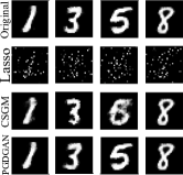
		Original Lasso CSGM PGD-GAN
(a)	(b)	(c)

Fig. 2: (a) Comparison of our algorithm with CSGM [17] and Lasso on MNIST; (b) Reconstruction results with $m=100$ measurements; (c) Reconstruction results on celebA dataset with $m=1000$ measurements.

From standard compressive sensing theory, we know that conditions such as the restricted isometry property (RIP) on $A$ are sufficient to guarantee robust signal recovery. It has also been demonstrated that the RIP is a sufficient condition for recovery using iterative projections on manifolds [37]. These conditions ensure that the operator $A$ preserves the uniqueness of the signal, i.e., the measurements corresponding to two different signals in the model would also be sufficiently different. In our case, we need to ensure that the difference vector of any two signals in the set ${\mathcal{S}}$ lies away from the nullspace of the matrix $A$. This condition is encoded via the S-REC (Set Restricted Eigenvalue Condition) defined in [17]. We slightly modify this condition and present it in the form of squared $l2$-norm :

Definition 2.1.

Let ${\mathcal{S}}\in{\mathbb{R}}^{n}$. $A$ is $m\times n$ matrix. For parameters $\gamma>0,~{}\delta\geq 0$, matrix $A$ is said to satisfy the S-REC$({\mathcal{S}},\gamma,\delta)$ if,

$$\|A(x_{1}-x_{2})\|^{2}\geq\gamma\|x_{1}-x_{2}\|^{2}-\delta,$$

for $\forall x_{1},x_{2}\in{\mathcal{S}}$.

Further, based on [37, 38], we propose the following theorem about the convergence of our algorithm:

Theorem 2.2.

Let $G:{\mathbb{R}}^{k}\rightarrow{\mathbb{R}}^{n}$ be a differentiable generator function with range ${\mathcal{S}}$. Let $A$ be a random Gaussian matrix with $A_{i,j}\sim N(0,1/m)$ such that it satisfies the S-REC$({\mathcal{S}},\gamma,\delta)$ with probability $1-p$, and has $\|Av\|\leq\rho\|v\|$ for every $v\in{\mathbb{R}}^{n}$ with probability $1-q$ with $\rho^{2}\leq\gamma$. Then, for every vector $x^{*}\in{\mathcal{S}}$, the sequence $\left(x_{t}\right)$ defined by the algorithm PGD-GAN [1] with $y=Ax^{*}$ converges to $x^{*}$ with probability at least $1-p-q$.

Proof.

Define the squared error loss function $\psi(v)\coloneqq\|y-Av\|^{2}$. Then, we have:

$$\psi(x_{t+1})-\psi(x_{t})$$

$$=\|Ax_{t+1}\|^{2}-2\langle y,Ax_{t+1}\rangle+2\langle y,Ax_{t}\rangle-\|Ax_{t}\|^{2},$$

$$=\|Ax_{t+1}-Ax_{t}\|^{2}+2\langle x_{t}-x_{t+1},A^{T}A(x^{*}-x_{t})\rangle.$$

Substituting $y=Ax^{*}$ and rearranging yields,

$$2\langle x_{t}-x_{t+1},A^{T}(y-Ax_{t})\rangle =\psi(x_{t+1})-\psi(x_{t})$$

$$-\|Ax_{t+1}-Ax_{t}\|^{2}.$$ (2.2)

Define:

$$w_{t}\coloneqq x_{t}+\eta A^{T}(y-Ax_{t})=x_{t}+\eta A^{T}A(x^{*}-x_{t})$$

Then, by definition of the projection operator $P_{G}$, the vector $x_{t+1}$ is a better (or equally good) approximation to $w$ as the true image $x^{*}$. Therefore, we have:

$$\|x_{t+1}-w_{t}\|^{2}\leq\|x^{*}-w_{t}\|^{2}.$$

Substituting for $w_{t}$ and expanding both sides, we get:

$$\|x_{t+1}-x_{t}\|^{2}-2\eta\langle x_{t+1}-x_{t},A^{T}(y-Ax_{t})\rangle$$

$$\leq\|x^{*}-x_{t}\|^{2}-2\eta\langle x^{*}-x_{t},A^{T}(y-Ax_{t})\rangle.$$

Substituting $y=Ax^{*}$ and rearranging yields,

$$2\langle x_{t}-x_{t+1},A^{T}(y-Ax_{t})\rangle$$

$$\leq\frac{1}{\eta}\|x^{*}-x_{t}\|^{2}-\frac{1}{\eta}\|x_{t+1}-x_{t}\|^{2}-2\psi(x_{t}).$$ (2.3)

We now use 2.2 and 2.3 to obtain,

$$\psi(x_{t+1})\leq\frac{1}{\eta}\|x^{*}-x_{t}\|^{2}-\psi(x_{t})$$

$$-\left(\frac{1}{\eta}\|x_{t+1}-x_{t}\|^{2}-\|Ax_{t+1}-Ax_{t}\|^{2}\right).$$ (2.4)

Now, from the S-REC, we know that,

$$\|A(x_{1}-x_{2})\|^{2}\geq\gamma\|x_{1}-x_{2}\|^{2}-\delta.$$

As $x^{*},x_{t}$ and $x_{t+1}$ are ‘natural’ vectors,

$$\frac{1}{\eta}\|x^{*}-x_{t}\|^{2}\leq\frac{1}{\eta\gamma}\|y-Ax_{t}\|^{2}+\frac{\delta}{\eta\gamma}.$$ (2.5)

Substituting 2.5 in 2.4,

$$\psi(x_{t+1})\leq\left(\frac{1}{\eta\gamma}-1\right)\psi(x_{t})$$

$$~{}~{}~{}~{}~{}~{}~{}-\left(\frac{1}{\eta}\|x_{t+1}-x_{t}\|^{2}-\|Ax_{t+1}-Ax_{t}\|^{2}\right)+\frac{\delta}{\eta\gamma}.$$

From our assumption that $\|Av\|\leq\rho\|v\|,\forall v\in{\mathbb{R}}^{n}$ with probability $1-q$, we write:

$$\|Ax_{t+1}-Ax_{t}\|^{2}\leq\rho^{2}\|x_{t+1}-x_{t}\|^{2},$$

$$\|Ax_{t+1}-Ax_{t}\|^{2}-\frac{1}{\eta}\|x_{t+1}-x_{t}\|^{2}\leq\left(\rho^{2}-\frac{1}{\eta}\right)\|x_{t+1}-x_{t}\|^{2}.$$

Let us choose learning rate$(\eta)$ such that $\frac{1}{2\gamma}<\eta<\frac{1}{\gamma}$. We also have $\rho^{2}\leq\gamma$. Combining both, we get $\rho^{2}<\frac{1}{\eta}$, which makes the L.H.S. in the above equation negative. Therefore,

$$\psi(x_{t+1})\leq\left(\frac{1}{\eta\gamma}-1\right)\psi(x_{t})+\frac{\delta}{\eta\gamma},$$

where $\delta$ is inversely proportional to the number of measurements $m$ [17]. Provided sufficient number of measurements, $\delta$ is small enough and can be ignored. Also, $\frac{1}{2\gamma}<\eta<\frac{1}{\gamma}$ yields,

$$0<\left(\frac{1}{\eta\gamma}-1\right)<1.$$

Hence,

$$\psi(x_{t+1})\leq\alpha\psi(x_{t});~{}0<\alpha<1,$$ (2.6)

with probability at least $1-p-q$. ∎

3 Models and Experiments

In this section, we describe our experimental setup and report the performance comparisons of our algorithm with that of [17] as well as the LASSO. We use two different GAN architectures and two different datasets in our experiments to show that our approach can work with variety of GAN architectures and datasets.

In our experiments, we choose the entries of the matrix $A$ independently from a Gaussian distribution with zero mean and $1/m$ standard deviation. We ignore the presence of noise; however, our experiments can be replicated with additive Gaussian noise. We use a gradient descent optimizer keeping the total number of update steps $(T\times T_{in})$ fixed for both algorithms and doesn’t allow random restarts.

In the first experiment, we use a very simple GAN model trained on the MNIST dataset, which is collection of $60,000$ handwritten digit images, each of size $28\times 28$ [18]. In our GAN, both the generator and the discriminator are fully-connected neural networks with only one hidden layer. The generator consists of $20$ input neurons, $200$ hidden-layer neurons and $784$ output neurons, while the discriminator consists of $784$ input neurons, $128$ hidden layer neurons and $1$ output neuron. The size of the latent space is set to $k=20$, i.e., the input to our generator is a standard normal vector $z\in R^{20}$. We train the GAN using the method described in [9]. We use the Adam optimizer [39] with learning rate $0.001$ and mini-batch size $128$ for the training.

We test the MNIST GAN with $10$ images taken from the span of generator to get rid of the representation error, and provide both quantitative and qualitative results. For PGD-GAN, because of the zero initialization, a high learning rate is required to get a meaningful output before passing it to the projection step. Therefore, we choose $\eta\geq 0.5$. The parameter $\eta_{in}$ is set to $0.01$ with $T=15$ and $T_{in}=200$. Thus, the total number of update steps is fixed to $3000$. Similarly, the algorithm of [17] is tested with $3000$ updates and $\eta=0.01$. For comparison, we use the reconstruction error $=\|\widehat{x}-x^{*}\|^{2}$. In Fig. 2(a), we show the reconstruction error comparisons for increasing values of number of measurements. We observe that our algorithm performs better than the other two methods. Also, as the input images are chosen from the span of the generator itself, it is possible to get close to zero error with only $100$ measurements. Fig. 2(b) depicts reconstruction results for selected MNIST images.

The second set of our experiments are performed on a Deep Convolutional GAN (DCGAN) trained on the celebA dataset, which contains more than $200,000$ face images of celebrities [21]. We use a pre-trained DCGAN model, which was made available by [17]. Thus, the details of the model and training are the same as described in [17]. The dimension of latent space for DCGAN is $k=100$. We report the results on a held out test dataset, unseen by the GAN at the time of training. Total number of updates is set to $1000$, with $T=10$ and $T_{in}=100$. Learning rates for PGD-GAN are set as $\eta=0.5$ and $\eta_{in}=0.1$. The algorithm of [17] is run with $\eta=0.1$ and $1000$ update steps. Image reconstruction results from $m=1000$ measurements with our algorithm are displayed in Fig. 2(c). We observe that our algorithm produces better reconstructions compared to the other baselines.

References

- [1] E. Candès et al., “Compressive sampling,” in Proc. of the intl. congress of math. Madrid, Spain, 2006, vol. 3, pp. 1433–1452.
- [2] E. Candes, J. Romberg, and T. Tao, “Stable signal recovery from incomplete and inaccurate measurements,” Comm. on pure and appl. math., vol. 59, no. 8, pp. 1207–1223, 2006.
- [3] D. Donoho, “Compressed sensing,” IEEE Trans. Inform. Theory, vol. 52, no. 4, pp. 1289–1306, 2006.
- [4] R. Baraniuk, V. Cevher, M. Duarte, and C. Hegde, “Model-based compressive sensing,” IEEE Trans. Inform. Theory, vol. 56, no. 4, pp. 1982–2001, Apr. 2010.
- [5] C. Hegde, P. Indyk, and L. Schmidt, “Fast algorithms for structured sparsity,” Bulletin of the EATCS, vol. 1, no. 117, pp. 197–228, Oct. 2015.
- [6] M. Elad and M. Aharon, “Image denoising via sparse and redundant representations over learned dictionaries,” IEEE Trans. Image Processing, vol. 15, no. 12, pp. 3736–3745, 2006.
- [7] M. Aharon, M. Elad, and A. Bruckstein, “-svd: An algorithm for designing overcomplete dictionaries for sparse representation,” IEEE Trans. Signal Processing, vol. 54, no. 11, pp. 4311–4322, 2006.
- [8] T. Chan, J. Shen, and H. Zhou, “Total variation wavelet inpainting,” Jour. of Math. imaging and Vision, vol. 25, no. 1, pp. 107–125, 2006.
- [9] I. Goodfellow, J. Pouget-Abadie, M. Mirza, B. Xu, D. Warde-Farley, S. Ozair, A. Courville, and Y. Bengio, “Generative adversarial nets,” in Proc. Adv. in Neural Processing Systems (NIPS), 2014, pp. 2672–2680.
- [10] J. Zhu, P. Krähenbühl, E. Shechtman, and A. Efros, “Generative visual manipulation on the natural image manifold,” in Proc. European Conf. Comp. Vision (ECCV), 2016.
- [11] A. Brock, T. Lim, J. Ritchie, and N. Weston, “Neural photo editing with introspective adversarial networks,” arXiv preprint arXiv:1609.07093, 2016.
- [12] X. Chen, Y. Duan, R. Houthooft, J. Schulman, I. Sutskever, and P. Abbeel, “Infogan: Interpretable representation learning by information maximizing generative adversarial nets,” in Proc. Adv. in Neural Processing Systems (NIPS), 2016, pp. 2172–2180.
- [13] J. Zhao, M. Mathieu, and Y. LeCun, “Energy-based generative adversarial network,” arXiv preprint arXiv:1609.03126, 2016.
- [14] D. Berthelot, T. Schumm, and L. Metz, “Began: Boundary equilibrium generative adversarial networks,” arXiv preprint arXiv:1703.10717, 2017.
- [15] R. Yeh, C. Chen, T. Lim, M. Hasegawa-Johnson, and M. Do, “Semantic image inpainting with perceptual and contextual losses,” arXiv preprint arXiv:1607.07539, 2016.
- [16] C. Ledig, L. Theis, F. Huszár, J. Caballero, A. Cunningham, A. Acosta, A. Aitken, A. Tejani, J. Totz, Z. Wang, et al., “Photo-realistic single image super-resolution using a generative adversarial network,” Proc. IEEE Conf. Comp. Vision and Pattern Recog. (CVPR), pp. 105–114, 2017.
- [17] A. Bora, A. Jalal, E. Price, and A. Dimakis, “Compressed sensing using generative models,” Proc. Int. Conf. Machine Learning, 2017.
- [18] Y. LeCun, L. on Bottou, Y. Bengio, and P. Haffner, “Gradient-based learning applied to document recognition,” Proc. of the IEEE, vol. 86, no. 11, pp. 2278–2324, 1998.
- [19] A. Radford, L. Metz, and S. Chintala, “Unsupervised representation learning with deep convolutional generative adversarial networks,” Proc. Int. Conf. Learning Representations (ICLR), 2016.
- [20] K. Taehoon, “A tensorflow implementation of “deep convolutional generative adversarial networks”,” 2017.
- [21] Z. Liu, P. Luo, X. Wang, and X. Tang, “Deep learning face attributes in the wild,” in Proc. of the IEEE Intl. Conf. on Comp. Vision, 2015, pp. 3730–3738.
- [22] D. Donoho, “De-noising by soft-thresholding,” IEEE Trans. Inform. Theory, vol. 41, no. 3, pp. 613–627, 1995.
- [23] Z. Xu and J. Sun, “Image inpainting by patch propagation using patch sparsity,” IEEE Trans. Image Processing, vol. 19, no. 5, pp. 1153–1165, 2010.
- [24] W. Dong, L. Zhang, G. Shi, and X. Wu, “Image deblurring and super-resolution by adaptive sparse domain selection and adaptive regularization,” IEEE Trans. Image Processing, vol. 20, no. 7, pp. 1838–1857, 2011.
- [25] L. Rudin, S. Osher, and E. Fatemi, “Nonlinear total variation based noise removal algorithms,” Physica D: Nonlinear Phenomena, vol. 60, no. 1-4, pp. 259–268, 1992.
- [26] A. Chambolle, “An algorithm for total variation minimization and applications,” Jour. of Math. imaging and vision, vol. 20, no. 1, pp. 89–97, 2004.
- [27] Y. LeCun, Y. Bengio, and G. Hinton, “Deep learning,” Nature, vol. 521, no. 7553, pp. 436–444, 2015.
- [28] K. Kulkarni, S. Lohit, P. Turaga, R. Kerviche, and A. Ashok, “Reconnet: Non-iterative reconstruction of images from compressively sensed measurements,” in Proc. IEEE Conf. Comp. Vision and Pattern Recog. (CVPR), 2016, pp. 449–458.
- [29] A. Mousavi, A. Patel, and R. Baraniuk, “A deep learning approach to structured signal recovery,” in Proc. Allerton Conf. Communication, Control, and Computing, 2015, pp. 1336–1343.
- [30] A. Mousavi and R. Baraniuk, “Learning to invert: Signal recovery via deep convolutional networks,” Proc. IEEE Int. Conf. Acoust., Speech, and Signal Processing (ICASSP), 2017.
- [31] L. Xu, J. Ren, C. Liu, and J. Jia, “Deep convolutional neural network for image deconvolution,” in Proc. Adv. in Neural Processing Systems (NIPS), 2014, pp. 1790–1798.
- [32] C. Dong, C. Loy, K. He, and X. Tang, “Image super-resolution using deep convolutional networks,” IEEE Trans. Pattern Anal. Machine Intell., vol. 38, no. 2, pp. 295–307, 2016.
- [33] J. Kim, J. Kwon Lee, and K. Mu Lee, “Accurate image super-resolution using very deep convolutional networks,” in Proc. IEEE Conf. Comp. Vision and Pattern Recog. (CVPR), 2016, pp. 1646–1654.
- [34] J. Rick Chang, C. Li, B. Poczos, B. Vijaya Kumar, and A. Sankaranarayanan, “One network to solve them all–solving linear inverse problems using deep projection models,” in Proc. IEEE Conf. Comp. Vision and Pattern Recog. (CVPR), 2017, pp. 5888–5897.
- [35] B. Kelly, T. Matthews, and M. Anastasio, “Deep learning-guided image reconstruction from incomplete data,” arXiv preprint arXiv:1709.00584, 2017.
- [36] M. Arjovsky, S. Chintala, and L. Bottou, “Wasserstein gan,” arXiv preprint arXiv:1701.07875, 2017.
- [37] P. Shah and V. Chandrasekaran, “Iterative projections for signal identification on manifolds: Global recovery guarantees,” in Proc. Allerton Conf. Communication, Control, and Computing, 2011, pp. 760–767.
- [38] S. Foucart and H. Rauhut, A mathematical introduction to compressive sensing, vol. 1, Springer.
- [39] D. Kingma and J. Ba, “Adam: A method for stochastic optimization,” arXiv preprint arXiv:1412.6980, 2014.