On the Gas Content and Efficiency of AGN Feedback in Low-redshift Quasars

Abstract

The interstellar medium is crucial to understanding the physics of active galaxies and the coevolution between supermassive black holes and their host galaxies. However, direct gas measurements are limited by sensitivity and other uncertainties. Dust provides an efficient indirect probe of the total gas. We apply this technique to a large sample of quasars, whose total gas content would be prohibitively expensive to measure. We present a comprehensive study of the full (1 to 500 µm) infrared spectral energy distributions of 87 redshift $<0.5$ quasars selected from the Palomar-Green sample, using photometric measurements from 2MASS, WISE, and Herschel, combined with Spitzer mid-infrared (5–40 µm) spectra. With a newly developed Bayesian Markov Chain Monte Carlo fitting method, we decompose various overlapping contributions to the integrated spectral energy distribution, including starlight, warm dust from the torus, and cooler dust on galaxy scales. This procedure yields a robust dust mass, which we use to infer the gas mass, using a gas-to-dust ratio constrained by the host galaxy stellar mass. Most ($90\%$) quasar hosts have gas fractions similar to those of massive, star-forming galaxies, although a minority ($10\%$) seem genuinely gas-deficient, resembling present-day massive early-type galaxies. This result indicates that “quasar mode” feedback does not occur or is ineffective in the host galaxies of low-redshift quasars. We also find that quasars can boost the interstellar radiation field and heat dust on galactic scales. This cautions against the common practice of using the far-infrared luminosity to estimate the host galaxy star formation rate.

1 Introduction

The tight correlation between the mass of supermassive black holes (BHs) and the bulge properties of their host galaxies (Magorrian et al., 1998; Ferrarese & Merritt, 2000; Gebhardt et al., 2000) implicates a strong connection between BH growth and galaxy evolution (Kormendy & Ho, 2013; Heckman & Best, 2014). However, the physical mechanisms behind this apparent BH–galaxy coevolution are still unclear. Energy feedback from active galactic nuclei (AGNs) is widely invoked to regulate galactic-scale star formation (Fabian, 2012). When accretion onto the BH reaches sufficiently high levels, such that the AGN is powerful enough to be regarded as a quasar, radiative or mechanical energy may drive a strong outflow that can blow the cold gas out of the galaxy (Silk & Rees, 1998). “Quasar mode” feedback may also play a central role in the popular gas-rich, major merger-driven evolutionary scenario for AGNs (Sanders et al., 1988), as they transform from an initially dust-enshrouded stage to their final unobscured quasar stage (Hopkins et al., 2008). Many modern cosmological simulations frequently invoke AGN feedback to effectively quench star formation in massive galaxies (e.g., Dubois et al. 2016; Weinberger et al. 2017).

From an observational perspective, however, it is still elusive when, where, and how AGNs influence their host galaxies. Is AGN feedback actually as pervasive as commonly assumed? Is it really as effective as we hope? Does AGN feedback suppress or, in fact, enhance star formation?

Recent studies offer a variety of promising, albeit ambiguous, clues. AGN outflows appear to be common at various redshifts (Perna et al., 2015; Woo et al., 2016; Nesvadba et al., 2017), but their contribution to feedback is unclear (Woo et al., 2017). Spatially resolved optical spectroscopy show that AGN winds may suppress star formation within the outflow, but they can also enhance star formation along the edges of the flow (e.g., Cresci et al. 2015; Carniani et al. 2016). Maiolino et al. (2017) argue that considerable star formation can be driven by outflows, which may also affect the overall morphology and kinematics of the galaxy. Submillimeter observations find strong outflows ($\gtrsim 100\,M_{\odot}$ yr^-1) in local ultraluminous infrared (IR) galaxies and AGNs (Cicone et al., 2014; Stone et al., 2016; González-Alfonso et al., 2017). However, the sample size is limited, and it is not clear whether the gas in the end actually gets blown out of the galaxy.

Independent of the specific details of the physical processes involved, AGN feedback, if it is effective enough to influence the host galaxy on large scales, ought to leave an imprint on the global cold interstellar medium (ISM) content of the system (Ho et al., 2008a). For example, in the merger-driven scenario realized in hydrodynamical simulations (e.g., Hopkins et al. 2006), broad-line (type 1) AGNs emerge in the aftermath of dust/gas expulsion by energy feedback, toward the end of the merger sequence. In such a scenario, we expect the cold ISM content in type 1 AGNs—especially those powerful enough to be deemed quasars—to be gas deficient relative to normal galaxies of similar mass. Is this true?

This basic, robust prediction has been difficult to test in practice because direct gas measurements are still lacking for large, well-defined samples of AGNs, particular those of sufficient luminosity to expect feedback processes to operate. Ho et al. (2008b) conducted the first systematic survey for H I gas in a large sample of nearby broad-line AGNs using the Arecibo telescope. Surprisingly, there is no evidence for gas deficit, casting doubt on the role of AGN feedback in these systems (Ho et al., 2008a). The sample of Ho et al., however, restricted to very low redshifts ($z\lesssim 0.1$) because of the limitations of current H I facilities, largely comprises relatively low-luminosity AGNs (Seyfert 1 galaxies), hardly powerful enough to qualify as bona fide quasars. Observations of the CO molecule can probe molecular gas in AGNs over a wide range of redshifts and luminosities, from relatively nearby lower luminosity sources (Scoville et al., 2003; Evans et al., 2006; Bertram et al., 2007; Husemann et al., 2017) to powerful quasars out to $z\gtrsim 6$ (e.g., Walter et al. 2004; Wang et al. 2013; Cicone et al. 2014; Wang et al. 2016b). However, CO observations are still relatively time consuming, precluding studies of large, statistically meaningful samples. Moreover, even when detected, the interpretation of the observations is still plagued by the uncertainty of the CO-to-$\mathrm{H}_{2}$ conversion factor $\alpha_{\mathrm{CO}}$ (Bolatto et al., 2013).

An alternative, independent strategy to probe the gas content of galaxies is to measure the dust mass, since these two constituents of the ISM are tightly linked through the gas-to-dust ratio ($\delta_{\mathrm{GDR}}$). This approach has been commonly and effectively exploited in a variety of studies, especially with the advent of the Herschel Space Observatory (Pilbratt et al., 2010), whose unprecedented sensitivity and angular resolution have furnished a wealth of far-IR (FIR) data for local and distant galaxies (e.g., Leroy et al. 2011; Dale et al. 2012; Eales et al. 2012; Berta et al. 2013, 2016) and AGNs (e.g., Leipski et al. 2014; Vito et al. 2014; Podigachoski et al. 2015; Westhues et al. 2016; Shimizu et al. 2017).

This paper analyzes IR spectral energy distributions (SEDs) of a large sample of bright, low-redshift quasars, using complete (1–500 µm), high-quality photometric measurements obtained from 2MASS, WISE, and Herschel, supplemented by mid-IR (MIR) spectroscopy over the wavelength range 5–40 µm from the Spitzer Infrared Spectrometer (IRS). The primary goal of this paper is to derive robust total dust masses for the sample, with well-understood uncertainties, carefully taking into account all known sources of systematic effects. To this end, we must decompose the IR SED into its three main constituents: stellar emission, AGN-heated dust emission, and host galaxy dust emission. We use the widely applied (e.g., Draine et al. 2007; Magdis et al. 2012; Ciesla et al. 2014) dust emission templates from Draine & Li (2007, hereafter DL07) to model the galactic dust emission. One of the major uncertainties comes from the treatment of the AGN dust torus emission, since it dominates the MIR and extends into the FIR (Nenkova et al., 2008a; Hönig & Kishimoto, 2010, 2017; Siebenmorgen et al., 2015; Xie et al., 2017). Our analysis takes full advantage of the important constraints on the torus emission provided by the IRS spectra. Many works have tried to decouple the galactic dust emission by decomposing the torus component from the observed IR SED. However, none of the current widely used codes (e.g., DecompIR, Mullaney et al. 2011; BayeSED, Han & Han 2014; CIGALE, Noll et al. 2009; Ciesla et al. 2015; AGNfitter, Calistro Rivera et al. 2016; but see Sales et al. 2015 and Herrero-Illana et al. 2017), properly fits spectroscopic data simultaneously with photometric data. Some study the spectra and the photometric SED separately (e.g., Marshall et al. 2007; Kirkpatrick et al. 2015). This approach, although practical, is not optimal, as it cannot provide a global, self-consistent solution with properly constrained uncertainties. We develop a new Bayesian Markov Chain Monte Carlo (MCMC) method that simultaneously incorporates photometric and spectral data in the fitting. We extensively evaluate a number of potential systematic uncertainties by comparing various methods to fit the SED.

We find evidence that quasars can heat dust on galactic scales. This implies that star formation rates traditionally estimated from the FIR may be biased by the AGN, even after accounting for the contribution from the torus emission. We derive robust dust masses for the host galaxies and use them to estimate the total mass of the cold gas. We show that the widely adopted method (e.g., Magdis et al. 2012; Santini et al. 2014; Berta et al. 2016) of estimating $\delta_{\mathrm{GDR}}$ from the galaxy stellar mass, in combination with other well-established galaxy scaling relations, provides reliable total gas masses within the main body of the galaxy (i.e., $\lesssim R_{25}$). We also present an empirical formalism to estimate the global gas content of the galaxy. We find that most quasar host galaxies have similar cold gas content to massive star-forming galaxies, although a minority are as gas poor as quenched elliptical galaxies. We argue that “quasar mode” feedback does not operate effectively in all quasar host galaxies.

The paper is organized as follows. We introduce the quasar and galaxy samples used in our study in Section 2. Section 3 describes the data reduction and construction of the SEDs for the quasar sample. Our method to model the SEDs with a newly developed Bayesian MCMC fitting algorithm is explained in Section 4, and the results of our measurements are presented in Section 5. Finally, in Section 6 we evaluate different methods to measure dust masses and discuss the implications of our results for AGN feedback. This work adopts the following parameters for a $\Lambda$CDM cosmology: $\Omega_{m}=0.308$, $\Omega_{\Lambda}=0.692$, and $H_{0}=67.8$ km s^-1 Mpc^-1 (Planck Collaboration et al., 2016).

2 Quasar and Galaxy Samples

We study the lower redshift ($z<0.5$) subset of 87 bright, UV/optically selected quasars from the Palomar-Green (PG) survey (Schmidt & Green, 1983), as summarized in Boroson & Green (1992). Although the PG quasar sample is not complete because of large photometric errors and its simple color selection criterion (e.g., Goldschmidt et al. 1992), this representative sample of bright, nearby quasars has been extensively studied for decades, allowing us to take advantage of a wealth of archival and literature multiwavelength data. As a major motivation of this study is to try to quantify, in as much detail as practical, various sources of systematic uncertainties in the derived dust properties, the availability of high-quality data across the entire IR (1 to 500 µm) region is crucial. The PG sample has the best and most complete set of IR observations for quasars or AGNs to date, encompassing not only six bands of Herschel photometry but also Spitzer IRS spectroscopy, and, of course, the full complement of shorter-wavelength measurements from the all-sky surveys of 2MASS and WISE (Section 3).

Equally importantly, the PG sample has available a rich repository of additional ancillary data from which critical physical properties of the central engine and host galaxy can be derived, including BH masses and Eddington ratios (optical spectra: Boroson & Green 1992; Ho & Kim 2009), accretion disk (X-ray spectra: Reeves & Turner 2000; Bianchi et al. 2009), jets (radio continuum: Kellermann et al. 1989, 1994), and host galaxy stellar morphology [Hubble Space Telescope (HST) images: Kim et al. 2008; Kim et al. 2017].

The physical properties of PG quasars are summarized in Table 1. Apart from properties related to the dust and ISM of the hosts, we also include information on the optical AGN luminosity, broad H$\beta$ line width, BH mass, and stellar mass of the host galaxies. Direct estimates of total stellar mass ($M_{*}$) are available for 55 objects for which Zhang et al. (2016) were able to analyze high-resolution optical and near-IR (NIR) images. For the remaining 32 objects that do not have direct estimates of stellar masses, we provide an indirect estimate of the lower limit for the total stellar mass from the bulge mass ($M_{\rm bulge}$), adopting the tight $M_{\mathrm{BH}}$–$M_{\mathrm{bulge}}$ relation of local inactive galaxies (Kormendy & Ho 2013; Equation (10)). We apply the recent calibration of Ho & Kim (2015, Equation (4)) to calculate single-epoch virial BH masses ($M_{\mathrm{BH}}$) using the 5100 Å monochromatic luminosity [$\lambda L_{\lambda}$(5100 Å)], adjusted to our cosmology, and the full width at half maximum (FWHM) of the broad H$\beta$ emission line (FWHM_Hβ), as listed in Vestergaard & Peterson (2006, Tables 1 and 7).

An integral part of our analysis will compare the ISM properties of PG quasars with those of local inactive galaxies (Section 5.3). We choose three samples of inactive galaxies.

1. KINGFISH (Kennicutt et al., 2011) consists of 61 representative local star-forming galaxies, with stellar masses measured using optical-to-NIR color and $H$-band luminosity (Skibba et al., 2011), assuming a Kroupa (2001) stellar IMF. The IR SEDs of the galaxies have been studied by Draine et al. (2007) and, more recently, Dale et al. (2012, 2017), using the DL07 model. The dust properties for most of the galaxies are reported in Draine et al. (2007), which we adopt.

2. The Herschel Reference Survey (HRS; Boselli et al. 2010) comprises 322 $K$-band selected galaxies within a distance of $D_{L}\approx$ 15–25 Mpc. The stellar masses were determined from the $i$-band luminosity with $g-i$ color-dependent stellar mass-to-light ratio from Zibetti et al. (2009), assuming the Chabrier (2003) stellar IMF. The ISM properties of HRS galaxies have been extensively studied (Cortese et al., 2012, 2016; Boselli et al., 2014b; Ciesla et al., 2014). Ciesla et al. (2014) measured dust properties by fitting DL07 models to the 8–500 µm SED using CIGALE. Boselli et al. (2014a) reported H I measurements, mainly from the Arecibo ALFALFA survey, and various CO(1–0) observations whereby the CO line fluxes were corrected according to the galaxy optical size. We adopt the molecular gas masses converted with a luminosity-dependent $\alpha_{\mathrm{CO}}$ conversion factor, considering that the stellar masses of the HRS galaxies span a wide range and the conversion factor varies with the gas-phase metallicity (and hence stellar mass; Boselli et al. 2002), although using a constant conversion factor only affects the molecular gas masses by, on average, $<0.1$ dex and makes essentially no difference in our results.

3. The COLD GASS (Saintonge et al., 2011) sample includes 366 nearby ($D_{L}\approx$ 100–200 Mpc) massive ($M_{*}>10^{10}\,M_{\odot}$; Saintonge et al. 2012) galaxies. The stellar masses come from SED fitting using photometric data from the Sloan Digital Sky Survey (SDSS; Stoughton et al. 2002) assuming the Chabrier (2003) stellar IMF. H I gas masses come from Arecibo data, and molecular gas masses were converted from CO(1–0) line luminosities measured using the IRAM 30 m telescope, assuming $\alpha_{\mathrm{CO}}=4.35$ $M_{\odot}\,\mathrm{(K\,km\,s^{-1}\,pc^{2})}^{-1}$. The gas masses for the COLD GASS and HRS samples account for elements heavier than hydrogen.

Table 1: Physical Properties of PG Quasars

Object	$z$	$D_{L}$	log $M_{*}$	log $\lambda L_{\lambda}$(5100 Å)	FWHMHβ	log $M_{\mathrm{BH}}$	log $M_{\mathrm{bulge}}$	log $U_{\mathrm{min}}$	$q_{\mathrm{PAH}}$	log $\gamma$	log $M_{d}$	log $\delta_{\mathrm{GDR}}$	log $M_{\mathrm{gas}}$		Radio
		(Mpc)	($M_{\odot}$)	(erg s-1)	(km s-1)	($M_{\odot}$)	($M_{\odot}$)		(%)		($M_{\odot}$)		($M_{\odot}$)
(1)	(2)	(3)	(4)	(5)	(6)	(7)	(8)	(9)	(10)	(11)	(12)	(13)	(14)		(15)
PG 0003$+$158	0.450	2572	$\cdots$	45.99	4751	9.45	11.65	$\cdots$	$\cdots$	$\cdots$	$<$8.9	2.09	$<$11.0		S
PG 0003$+$199	0.025	113	$\cdots$	44.17	1585	7.52	10.00	+$1.18_{-0.00}^{+0.00}$	$1.77_{-0.65}^{+0.00}$	$-3.76_{-0.58}^{+0.52}$	$6.23_{-0.03}^{+0.04}$	2.09	8.32$\pm$	0.20	Q
PG 0007$+$106	0.089	420	10.84	44.79	5085	8.87	11.15	+$0.90_{-0.06}^{+0.10}$	$1.12_{-0.00}^{+0.00}$	$-4.39_{-0.27}^{+0.30}$	$7.67_{-0.13}^{+0.07}$	2.09	9.76$\pm$	0.22	F
PG 0026$+$129	0.142	693	10.88	45.07	1821	8.12	10.52	+$1.30_{-0.12}^{+0.10}$	$0.47_{-0.00}^{+0.65}$	$-3.06_{-0.55}^{+0.61}$	$6.81_{-0.08}^{+0.11}$	2.09	8.90$\pm$	0.22	Q
PG 0043$+$039	0.384	2133	10.94	45.51	5291	9.28	11.51	$\cdots$	$\cdots$	$\cdots$	$<$8.6	2.09	$<$10.7		Q
PG 0049$+$171	0.064	297	$\cdots$	43.97	5234	8.45	10.80	+$0.60_{-0.30}^{+0.24}$	$0.47_{-0.00}^{+0.65}$	$-4.00_{-0.69}^{+0.97}$	$6.57_{-0.30}^{+0.30}$	2.09	8.66$\pm$	0.36	Q
PG 0050$+$124	0.061	282	11.12	44.76	1171	7.57	10.05	+$1.00_{-0.00}^{+0.00}$	$0.47_{-0.00}^{+0.00}$	$-3.16_{-0.53}^{+0.46}$	$8.22_{-0.01}^{+0.01}$	2.08	10.30$\pm$	0.20	Q
PG 0052$+$251	0.155	763	11.05	45.00	5187	8.99	11.26	+$0.60_{-0.00}^{+0.00}$	$2.50_{-0.73}^{+0.00}$	$-3.90_{-0.68}^{+0.87}$	$8.21_{-0.02}^{+0.02}$	2.08	10.29$\pm$	0.20	Q
PG 0157$+$001	0.164	811	11.53	44.95	2432	8.31	10.68	+$1.18_{-0.10}^{+0.00}$	$0.47_{-0.00}^{+0.00}$	$-1.07_{-0.09}^{+0.08}$	$8.69_{-0.02}^{+0.03}$	2.11	10.80$\pm$	0.20	Q
PG 0804$+$761	0.100	475	10.64	45.03	3045	8.55	10.88	+$1.40_{-0.10}^{+0.00}$	$0.47_{-0.00}^{+0.65}$	$-1.87_{-0.56}^{+0.42}$	$6.68_{-0.05}^{+0.06}$	2.11	8.79$\pm$	0.21	Q
PG 0838$+$770	0.131	635	11.14	44.70	2764	8.29	10.66	+$0.70_{-0.00}^{+0.00}$	$0.47_{-0.00}^{+0.00}$	$-1.34_{-0.20}^{+0.13}$	$8.13_{-0.02}^{+0.02}$	2.08	10.21$\pm$	0.20	Q
PG 0844$+$349	0.064	297	10.69	44.46	2386	8.03	10.44	+$0.00_{-0.00}^{+0.08}$	$1.77_{-0.00}^{+0.73}$	$-4.68_{-0.24}^{+0.42}$	$7.91_{-0.08}^{+0.03}$	2.11	10.01$\pm$	0.21	Q
PG 0921$+$525	0.035	159	$\cdots$	43.60	2079	7.45	09.94	+$0.60_{-0.00}^{+0.10}$	$0.47_{-0.00}^{+0.65}$	$-2.86_{-0.44}^{+0.32}$	$6.76_{-0.07}^{+0.02}$	2.09	8.85$\pm$	0.21	Q
PG 0923$+$201	0.190	955	11.09	45.01	7598	9.33	11.55	+$1.30_{-0.00}^{+0.10}$	$1.77_{-0.65}^{+0.73}$	$-3.05_{-1.03}^{+0.96}$	$6.91_{-0.09}^{+0.10}$	2.08	9.00$\pm$	0.22	Q
PG 0923$+$129	0.029	131	$\cdots$	43.83	1957	7.52	10.00	+$0.85_{-0.00}^{+0.00}$	$0.47_{-0.00}^{+0.65}$	$-1.66_{-0.14}^{+0.08}$	$7.39_{-0.01}^{+0.01}$	2.09	9.48$\pm$	0.20	Q
PG 0934$+$013	0.050	229	$\cdots$	43.85	1254	7.15	09.68	+$0.70_{-0.00}^{+0.00}$	$1.12_{-0.00}^{+0.00}$	$-1.41_{-0.08}^{+0.09}$	$7.39_{-0.02}^{+0.02}$	2.09	9.48$\pm$	0.20	Q
PG 0947$+$396	0.206	1045	10.73	44.78	4817	8.81	11.11	+$0.85_{-0.24}^{+0.23}$	$1.12_{-0.65}^{+0.65}$	$-4.05_{-0.66}^{+0.82}$	$7.71_{-0.18}^{+0.21}$	2.10	9.81$\pm$	0.28	Q
PG 0953$+$414	0.239	1235	11.16	45.35	3111	8.74	11.04	+$0.60_{-0.20}^{+0.30}$	$1.77_{-0.65}^{+0.73}$	$-4.41_{-0.43}^{+0.74}$	$7.97_{-0.30}^{+0.27}$	2.08	10.05$\pm$	0.35	Q
PG 1001$+$054	0.161	795	10.47	44.71	1700	7.87	10.30	+$0.90_{-0.20}^{+0.18}$	$1.77_{-0.65}^{+0.73}$	$-1.30_{-0.40}^{+0.26}$	$7.37_{-0.21}^{+0.20}$	2.13	9.51$\pm$	0.29	Q
PG 1004$+$130	0.240	1240	11.44	45.51	6290	9.43	11.64	+$1.30_{-0.00}^{+0.00}$	$0.47_{-0.00}^{+0.00}$	$-2.51_{-0.51}^{+0.46}$	$7.72_{-0.04}^{+0.04}$	2.10	9.82$\pm$	0.20	S
PG 1011$-$040	0.058	268	$\cdots$	44.23	1381	7.43	09.93	+$0.60_{-0.00}^{+0.00}$	$0.47_{-0.00}^{+0.00}$	$-1.61_{-0.17}^{+0.11}$	$7.56_{-0.01}^{+0.02}$	2.09	9.65$\pm$	0.20	Q
PG 1012$+$008	0.185	927	11.15	44.98	2615	8.39	10.74	+$0.70_{-0.00}^{+0.00}$	$0.47_{-0.00}^{+0.65}$	$-1.21_{-0.21}^{+0.13}$	$8.12_{-0.03}^{+0.04}$	2.08	10.20$\pm$	0.20	Q
PG 1022$+$519	0.045	206	$\cdots$	43.67	1566	7.25	09.77	+$0.85_{-0.00}^{+0.00}$	$1.77_{-0.00}^{+0.00}$	$-1.48_{-0.04}^{+0.03}$	$7.25_{-0.01}^{+0.01}$	2.09	9.34$\pm$	0.20	Q
PG 1048$+$342	0.167	828	10.77	44.68	3581	8.50	10.84	+$0.40_{-0.10}^{+0.20}$	$0.47_{-0.00}^{+0.65}$	$-2.15_{-0.55}^{+0.32}$	$8.04_{-0.16}^{+0.15}$	2.10	10.14$\pm$	0.25	Q
PG 1048$-$090	0.344	1875	$\cdots$	45.57	5611	9.37	11.58	$\cdots$	$\cdots$	$\cdots$	$<$8.5	2.09	$<$10.6		S
PG 1049$-$005	0.357	1958	$\cdots$	45.60	5351	9.34	11.56	+$1.40_{-0.10}^{+0.00}$	$1.77_{-0.00}^{+0.00}$	$-4.57_{-0.29}^{+0.38}$	$8.34_{-0.04}^{+0.05}$	2.09	10.44$\pm$	0.20	Q
PG 1100$+$772	0.313	1681	11.27	45.55	6151	9.44	11.64	+$0.60_{-0.12}^{+0.10}$	$0.47_{-0.00}^{+0.00}$	$-0.48_{-0.16}^{+0.22}$	$8.17_{-0.17}^{+0.11}$	2.09	10.26$\pm$	0.24	S
PG 1103$-$006	0.425	2404	$\cdots$	45.64	6183	9.49	11.68	$\cdots$	$\cdots$	$\cdots$	$<$8.4	2.09	$<$10.5		S
PG 1114$+$445	0.144	704	$\cdots$	44.70	4554	8.72	11.03	$-0.82_{-0.18}^{+0.30}$	$4.58_{-0.68}^{+0.00}$	$-4.57_{-0.31}^{+0.56}$	$8.38_{-0.37}^{+0.24}$	2.09	10.47$\pm$	0.36	Q
PG 1115$+$407	0.154	757	$\cdots$	44.59	1679	7.80	10.24	+$0.70_{-0.00}^{+0.00}$	$1.12_{-0.00}^{+0.00}$	$-1.48_{-0.03}^{+0.04}$	$8.44_{-0.01}^{+0.01}$	2.09	10.53$\pm$	0.20	Q
PG 1116$+$215	0.177	882	10.61	45.37	2897	8.69	11.00	+$1.40_{-0.10}^{+0.00}$	$1.12_{-0.65}^{+0.65}$	$-2.83_{-0.63}^{+0.65}$	$7.26_{-0.05}^{+0.08}$	2.11	9.38$\pm$	0.21	Q
PG 1119$+$120	0.049	225	10.67	44.10	1773	7.58	10.05	+$1.08_{-0.00}^{+0.00}$	$0.47_{-0.00}^{+0.65}$	$-1.35_{-0.12}^{+0.10}$	$7.16_{-0.02}^{+0.02}$	2.11	9.26$\pm$	0.20	Q
PG 1121$+$422	0.234	1205	10.29	44.85	2192	8.17	10.55	$\cdots$	$\cdots$	$\cdots$	$<$8.4	2.16	$<$10.6		Q
PG 1126$-$041	0.060	277	10.85	44.36	2111	7.87	10.30	+$1.08_{-0.00}^{+0.00}$	$0.47_{-0.00}^{+0.00}$	$-1.57_{-0.33}^{+0.17}$	$7.56_{-0.02}^{+0.01}$	2.09	9.65$\pm$	0.20	Q
PG 1149$-$110	0.049	225	$\cdots$	44.08	3032	8.04	10.44	+$0.70_{-0.00}^{+0.00}$	$0.47_{-0.00}^{+0.00}$	$-1.51_{-0.12}^{+0.10}$	$7.40_{-0.02}^{+0.02}$	2.09	9.49$\pm$	0.20	Q
PG 1151$+$117	0.176	877	10.45	44.73	4284	8.68	10.99	$\cdots$	$\cdots$	$\cdots$	$<$7.9	2.14	$<$10.0		Q
PG 1202$+$281	0.165	817	10.86	44.57	5036	8.74	11.04	+$1.40_{-0.00}^{+0.00}$	$3.19_{-0.69}^{+0.71}$	$-2.08_{-0.61}^{+0.44}$	$7.41_{-0.02}^{+0.04}$	2.09	9.51$\pm$	0.20	Q
PG 1211$+$143	0.085	400	10.38	45.04	1817	8.10	10.50	+$0.30_{-0.22}^{+0.18}$	$4.58_{-0.68}^{+0.00}$	$-4.57_{-0.27}^{+0.49}$	$7.36_{-0.22}^{+0.20}$	2.15	9.51$\pm$	0.29	Q
PG 1216$+$069	0.334	1812	10.85	45.69	5180	9.36	11.57	$\cdots$	$\cdots$	$\cdots$	$<$8.3	2.09	$<$10.4		Q
PG 1226$+$023	0.158	779	11.51	45.99	3500	9.18	11.42	$-0.40_{-0.30}^{+0.30}$	$3.90_{-0.71}^{+0.68}$	$-2.15_{-0.66}^{+0.72}$	$7.00_{-0.50}^{+0.56}$	2.10	9.11$\pm$	0.57	F
PG 1229$+$204	0.064	297	10.94	44.35	3335	8.26	10.63	+$0.60_{-0.00}^{+0.00}$	$0.47_{-0.00}^{+0.65}$	$-3.09_{-0.86}^{+0.73}$	$7.63_{-0.02}^{+0.02}$	2.09	9.72$\pm$	0.20	Q
PG 1244$+$026	0.048	220	$\cdots$	43.77	0721	6.62	09.23	+$1.18_{-0.00}^{+0.00}$	$0.47_{-0.00}^{+0.00}$	$-1.07_{-0.04}^{+0.04}$	$6.69_{-0.02}^{+0.02}$	2.09	8.78$\pm$	0.20	Q
PG 1259$+$593	0.472	2723	10.99	45.88	3377	9.09	11.34	+$0.40_{-0.32}^{+0.45}$	$1.12_{-0.65}^{+0.65}$	$-0.13_{-0.16}^{+0.09}$	$7.80_{-0.36}^{+0.36}$	2.08	9.89$\pm$	0.41	Q
PG 1302$-$102	0.286	1515	11.23	45.80	3383	9.05	11.31	+$0.90_{-0.06}^{+0.00}$	$0.47_{-0.00}^{+0.00}$	$-0.45_{-0.13}^{+0.18}$	$7.87_{-0.15}^{+0.12}$	2.08	9.96$\pm$	0.24	F
PG 1307$+$085	0.155	763	10.78	44.98	5307	9.00	11.27	+$0.90_{-0.20}^{+0.18}$	$3.90_{-0.71}^{+0.68}$	$-3.27_{-0.87}^{+0.80}$	$7.46_{-0.17}^{+0.18}$	2.10	9.56$\pm$	0.26	Q
PG 1309$+$355	0.184	921	11.22	44.98	2917	8.48	10.82	+$0.40_{-0.10}^{+0.08}$	$3.90_{-0.71}^{+0.00}$	$-3.61_{-0.67}^{+0.72}$	$8.32_{-0.11}^{+0.11}$	2.08	10.40$\pm$	0.23	F
PG 1310$-$108	0.035	159	$\cdots$	43.70	3606	7.99	10.40	+$0.60_{-0.00}^{+0.00}$	$2.50_{-0.00}^{+0.69}$	$-4.79_{-0.14}^{+0.26}$	$6.86_{-0.02}^{+0.02}$	2.09	8.95$\pm$	0.20	Q
PG 1322$+$659	0.168	833	10.61	44.95	2765	8.42	10.77	+$1.40_{-0.00}^{+0.00}$	$3.19_{-0.69}^{+0.00}$	$-1.96_{-0.43}^{+0.34}$	$7.35_{-0.03}^{+0.05}$	2.11	9.47$\pm$	0.20	Q
PG 1341$+$258	0.087	410	$\cdots$	44.31	3014	8.15	10.54	+$0.70_{-0.10}^{+0.15}$	$1.12_{-0.00}^{+0.65}$	$-1.28_{-0.23}^{+0.16}$	$7.23_{-0.19}^{+0.11}$	2.09	9.32$\pm$	0.25	Q
PG 1351$+$236	0.055	253	$\cdots$	44.02	6527	8.67	10.98	+$0.85_{-0.00}^{+0.00}$	$2.50_{-0.00}^{+0.00}$	$-1.87_{-0.12}^{+0.08}$	$7.68_{-0.02}^{+0.01}$	2.09	9.77$\pm$	0.20	Q
PG 1351$+$640	0.087	410	10.63	44.81	5646	8.97	11.24	+$1.40_{-0.00}^{+0.00}$	$1.12_{-0.00}^{+0.00}$	$-1.48_{-0.24}^{+0.17}$	$7.56_{-0.01}^{+0.01}$	2.11	9.67$\pm$	0.20	Q
PG 1352$+$183	0.158	779	10.49	44.79	3581	8.56	10.89	$\cdots$	$\cdots$	$\cdots$	$<$7.9	2.13	$<$10.0		Q
PG 1354$+$213	0.300	1600	10.97	44.95	4127	8.77	11.07	+$0.70_{-0.30}^{+0.38}$	$1.12_{-0.65}^{+0.65}$	$-3.16_{-1.10}^{+1.30}$	$7.76_{-0.40}^{+0.39}$	2.09	9.84$\pm$	0.44	Q
PG 1402$+$261	0.164	811	10.86	44.95	1874	8.08	10.48	+$1.30_{-0.00}^{+0.00}$	$0.47_{-0.00}^{+0.00}$	$-1.36_{-0.13}^{+0.11}$	$7.83_{-0.02}^{+0.02}$	2.09	9.93$\pm$	0.20	Q
PG 1404$+$226	0.098	465	$\cdots$	44.35	0787	7.01	09.56	+$0.18_{-0.00}^{+0.00}$	$1.12_{-0.00}^{+0.00}$	$-1.33_{-0.06}^{+0.06}$	$7.89_{-0.03}^{+0.03}$	2.09	9.99$\pm$	0.20	Q
PG 1411$+$442	0.089	420	10.84	44.60	2640	8.20	10.58	+$0.40_{-0.00}^{+0.08}$	$1.77_{-0.65}^{+0.73}$	$-1.25_{-0.14}^{+0.12}$	$7.81_{-0.05}^{+0.04}$	2.09	9.90$\pm$	0.21	Q
PG 1415$+$451	0.114	546	$\cdots$	44.53	2591	8.14	10.53	+$1.00_{-0.00}^{+0.00}$	$2.50_{-0.00}^{+0.00}$	$-1.79_{-0.17}^{+0.14}$	$7.64_{-0.02}^{+0.02}$	2.09	9.73$\pm$	0.20	Q
PG 1416$-$129	0.129	624	$\cdots$	45.11	6098	9.19	11.43	+$1.40_{-0.10}^{+0.00}$	$2.50_{-0.00}^{+0.69}$	$-3.94_{-0.64}^{+0.79}$	$7.02_{-0.04}^{+0.09}$	2.09	9.11$\pm$	0.21	Q
PG 1425$+$267	0.366	2016	11.15	45.73	9405	9.90	12.04	+$1.40_{-0.10}^{+0.00}$	$0.47_{-0.00}^{+0.00}$	$-1.01_{-0.28}^{+0.25}$	$7.75_{-0.06}^{+0.06}$	2.08	9.83$\pm$	0.21	S
PG 1426$+$015	0.086	405	11.05	44.85	6808	9.15	11.39	+$0.70_{-0.00}^{+0.00}$	$0.47_{-0.00}^{+0.00}$	$-1.23_{-0.07}^{+0.06}$	$7.92_{-0.01}^{+0.01}$	2.08	10.00$\pm$	0.20	Q
PG 1427$+$480	0.221	1130	10.77	44.73	2515	8.22	10.60	+$1.40_{-0.10}^{+0.00}$	$1.77_{-0.65}^{+0.00}$	$-2.79_{-0.80}^{+0.75}$	$7.42_{-0.07}^{+0.09}$	2.10	9.52$\pm$	0.22	Q
PG 1435$-$067	0.129	624	10.51	44.89	3157	8.50	10.84	+$0.00_{-0.30}^{+0.18}$	$3.19_{-0.69}^{+0.71}$	$-1.56_{-0.44}^{+0.32}$	$7.84_{-0.27}^{+0.31}$	2.13	9.97$\pm$	0.35	Q
PG 1440$+$356	0.077	360	11.05	44.52	1394	7.60	10.07	+$1.18_{-0.00}^{+0.00}$	$1.77_{-0.00}^{+0.00}$	$-2.46_{-0.38}^{+0.32}$	$7.87_{-0.01}^{+0.01}$	2.08	9.95$\pm$	0.20	Q
PG 1444$+$407	0.267	1400	11.15	45.17	2457	8.44	10.78	+$1.30_{-0.00}^{+0.00}$	$0.47_{-0.00}^{+0.00}$	$-0.60_{-0.16}^{+0.17}$	$7.43_{-0.15}^{+0.13}$	2.08	9.51$\pm$	0.24	Q
PG 1448$+$273	0.065	301	$\cdots$	44.45	0815	7.09	09.63	+$1.18_{-0.00}^{+0.00}$	$2.50_{-0.73}^{+0.69}$	$-4.33_{-0.46}^{+0.76}$	$7.08_{-0.03}^{+0.02}$	2.09	9.17$\pm$	0.20	Q
PG 1501$+$106	0.036	164	$\cdots$	44.26	5454	8.64	10.96	+$1.30_{-0.00}^{+0.10}$	$0.47_{-0.00}^{+0.00}$	$-1.55_{-0.48}^{+0.30}$	$6.60_{-0.05}^{+0.04}$	2.09	8.69$\pm$	0.20	Q
PG 1512$+$370	0.371	2048	11.01	45.57	6803	9.53	11.72	+$0.40_{-0.22}^{+0.20}$	$1.12_{-0.65}^{+0.65}$	$-2.50_{-0.80}^{+0.67}$	$8.44_{-0.25}^{+0.22}$	2.08	10.52$\pm$	0.31	S
PG 1519$+$226	0.137	666	$\cdots$	44.68	2187	8.07	10.47	+$1.00_{-0.00}^{+0.00}$	$1.12_{-0.00}^{+0.65}$	$-1.42_{-0.20}^{+0.16}$	$7.54_{-0.04}^{+0.03}$	2.09	9.63$\pm$	0.20	Q
PG 1534$+$580	0.030	136	$\cdots$	43.66	5324	8.30	10.67	+$1.08_{-0.08}^{+0.00}$	$2.50_{-0.73}^{+0.00}$	$-3.29_{-0.89}^{+0.84}$	$6.42_{-0.04}^{+0.06}$	2.09	8.51$\pm$	0.21	Q
PG 1535$+$547	0.038	173	$\cdots$	43.93	1420	7.30	09.81	$-0.10_{-0.06}^{+0.00}$	$1.12_{-0.00}^{+0.00}$	$-0.92_{-0.08}^{+0.09}$	$7.21_{-0.07}^{+0.05}$	2.09	9.31$\pm$	0.21	Q
PG 1543$+$489	0.400	2237	10.93	45.42	1529	8.16	10.54	+$1.40_{-0.00}^{+0.00}$	$0.47_{-0.00}^{+0.65}$	$-2.52_{-0.50}^{+0.43}$	$8.50_{-0.04}^{+0.04}$	2.09	10.59$\pm$	0.20	Q
PG 1545$+$210	0.266	1394	11.15	45.40	7022	9.47	11.67	$\cdots$	$\cdots$	$\cdots$	$<$8.3	2.08	$<$10.4		S
PG 1552$+$085	0.119	572	$\cdots$	44.67	1377	7.67	10.12	$-0.30_{-0.00}^{+0.00}$	$1.12_{-0.65}^{+0.00}$	$-0.26_{-0.21}^{+0.17}$	$7.64_{-0.17}^{+0.19}$	2.09	9.73$\pm$	0.27	Q
PG 1612$+$261	0.131	635	$\cdots$	44.69	2491	8.19	10.57	+$1.00_{-0.10}^{+0.08}$	$1.12_{-0.00}^{+0.00}$	$-4.72_{-0.21}^{+0.39}$	$7.91_{-0.09}^{+0.07}$	2.09	10.00$\pm$	0.22	Q
PG 1613$+$658	0.129	624	11.46	44.81	8441	9.32	11.54	+$1.00_{-0.00}^{+0.00}$	$0.47_{-0.00}^{+0.00}$	$-1.23_{-0.05}^{+0.05}$	$8.46_{-0.01}^{+0.01}$	2.10	10.56$\pm$	0.20	Q
PG 1617$+$175	0.114	546	10.47	44.81	5316	8.91	11.19	+$0.85_{-0.15}^{+0.23}$	$0.47_{-0.00}^{+0.65}$	$-0.95_{-0.36}^{+0.19}$	$6.87_{-0.17}^{+0.14}$	2.13	9.00$\pm$	0.25	Q
PG 1626$+$554	0.133	645	10.84	44.55	4474	8.63	10.95	$\cdots$	$\cdots$	$\cdots$	$<$7.5	2.09	$<$9.6		Q
PG 1700$+$518	0.282	1490	11.39	45.69	2185	8.61	10.93	+$1.18_{-0.00}^{+0.00}$	$0.47_{-0.00}^{+0.00}$	$-0.89_{-0.11}^{+0.09}$	$8.55_{-0.02}^{+0.02}$	2.09	10.64$\pm$	0.20	Q
PG 1704$+$608	0.371	2048	11.52	45.67	6552	9.55	11.74	+$1.40_{-0.00}^{+0.00}$	$0.47_{-0.00}^{+0.65}$	$-3.23_{-0.54}^{+0.52}$	$8.16_{-0.03}^{+0.04}$	2.11	10.26$\pm$	0.20	S
PG 2112$+$059	0.466	2681	$\cdots$	46.16	3176	9.18	11.42	+$0.85_{-0.00}^{+0.15}$	$0.47_{-0.00}^{+0.65}$	$-0.70_{-0.16}^{+0.15}$	$8.50_{-0.09}^{+0.09}$	2.09	10.59$\pm$	0.22	Q
PG 2130$+$099	0.061	282	10.85	44.54	2294	8.04	10.44	+$0.90_{-0.00}^{+0.00}$	$0.47_{-0.00}^{+0.65}$	$-1.44_{-0.13}^{+0.11}$	$7.60_{-0.01}^{+0.02}$	2.09	9.69$\pm$	0.20	Q
PG 2209$+$184	0.070	326	$\cdots$	44.44	6488	8.89	11.17	+$0.08_{-0.00}^{+0.00}$	$2.50_{-0.00}^{+0.69}$	$-1.91_{-0.19}^{+0.13}$	$7.98_{-0.05}^{+0.04}$	2.09	10.07$\pm$	0.20	F
PG 2214$+$139	0.067	311	10.98	44.63	4532	8.68	10.99	+$0.40_{-0.10}^{+0.08}$	$3.90_{-0.71}^{+0.68}$	$-2.90_{-0.54}^{+0.47}$	$7.48_{-0.06}^{+0.07}$	2.08	9.56$\pm$	0.21	Q
PG 2233$+$134	0.325	1755	10.81	45.30	1709	8.19	10.57	+$0.60_{-0.20}^{+0.10}$	$1.77_{-0.65}^{+0.73}$	$-4.51_{-0.33}^{+0.67}$	$8.36_{-0.16}^{+0.21}$	2.09	10.46$\pm$	0.27	Q
PG 2251$+$113	0.323	1743	11.05	45.66	4147	9.15	11.39	+$1.30_{-0.12}^{+0.10}$	$2.50_{-0.73}^{+0.69}$	$-3.59_{-0.74}^{+0.83}$	$7.63_{-0.11}^{+0.15}$	2.08	9.71$\pm$	0.24	S
PG 2304$+$042	0.042	192	$\cdots$	44.04	6487	8.68	10.99	+$0.70_{-0.22}^{+0.15}$	$1.12_{-0.65}^{+0.65}$	$-4.40_{-0.45}^{+0.68}$	$6.28_{-0.17}^{+0.20}$	2.09	8.37$\pm$	0.27	Q
PG 2308$+$098	0.432	2451	$\cdots$	45.75	7914	9.76	11.92	$\cdots$	$\cdots$	$\cdots$	$<$8.9	2.09	$<$11.0		S

Note. — (1) Object name. (2) Redshift. (3) The luminosity distance calculated with $\Omega_{m}=0.308$, $\Omega_{\Lambda}=0.692$, and $H_{0}=67.8$ km s^-1 Mpc^-1 (Planck Collaboration et al., 2016). (4) The stellar mass of the quasar host galaxies from Zhang et al. (2016). In order to convert from the Salpeter (1955) IMF to the Kroupa-like IMF, we divide the stellar mass by 1.5, following Zhang et al. (2016). (5) The monochromatic luminosity at 5100 Å. (6) The FWHM of the broad H$\beta$ emission line. (7) The mass of the BH. (8) The stellar bulge mass of the host galaxy estimated from $M_{\mathrm{BH}}$. (9) The best-fit minimum intensity of the interstellar radiation field relative to that measured in the solar neighborhood. (10) The best-fit mass fraction of the dust in the form of PAH molecules. (11) The best-fit mass fraction of the dust associated with the power-law part of the interstellar radiation field. (12) The best-fit total dust mass. The quoted uncertainties of the DL07 model represent the 68% confidence level determined from the 16th and 84th percentile of the marginalized posterior PDF. However, for $U_{\mathrm{min}}$ or $q_{\mathrm{PAH}}$, if fewer than 16% of the sampled values at the discrete grids lie below (above) the best-fit value, the lower (upper) uncertainty of the parameter is not resolved, and it is reported as “0.00” in the table. (13) The gas-to-dust ratio of the galaxy, estimated from the host galaxy stellar mass. For objects without a stellar mass measured, the median value of the sample is adopted, 124$\pm$6. The value of $\delta_{\mathrm{GDR}}$ has been corrected using Equation (17), so that the total gas mass can be compared to the directly measured gas mass in an unbiased manner. (14) The total gas mass with uncertainty, combining the uncertainties of the dust mass and the $\delta_{\mathrm{GDR}}$ (0.2 dex). (15) The radio type of the quasar: “Q” for radio-quiet source, “S” for steep-spectrum source, and “F” for flat-spectrum source.

3 Data Analysis and Compilation

3.1 2MASS and WISE

The 2MASS (Skrutskie et al., 2006) $J$ (1.235 $\mu$m), $H$ (1.662 $\mu$m), and $K_{s}$ (2.159 $\mu$m) bands (Cohen et al., 2003) are dominated by emission from the old stellar population of the host galaxy. Since the quasar host galaxies may be resolved, the measurements from the 2MASS Point Source Catalog are not accurate. At the same time, only a small fraction of the PG quasars are included in the 2MASS Extended Source Catalog. Therefore, we reanalyze the 2MASS data for the entire sample. We collect the 2MASS images from the NASA/IPAC Infrared Science Archive (IRSA) by matching each source with a search radius of $4\arcsec$ with respect to the optical position of the quasar and performing aperture photometry using the Python package photutils. To measure the integrated flux, we use the default aperture radius of 7″ (Jarrett et al., 2003) with the sky annulus set to a radius of 25″ to 35″. For the nearest ($z\lesssim 0.1$) quasars having more extended host galaxies, we use a larger aperture radius of $20\arcsec$ but the same sky annulus. To determine the uncertainty, we perform 500 random aperture measurements of the sky, in exactly the same way as the quasar, with all sources masked, and use the standard deviation of the spatial variation of the sky to be the uncertainty of our measurement. We do not apply any aperture correction, which is found to be very small. The apertures of five targets (PG 0921$+$525, PG 1115$+$407, PG 1216$+$069, PG 1534$+$580, and PG 1612+261) are affected by projected close companions. As all the companions are $\gtrsim 4\arcsec$ away from the quasars, we first use GALFIT (Peng et al., 2002, 2010) to fit and remove them from the images. The point-spread function (PSF) of each image is derived from the stars in the field using DAOPHOT in IRAF (Tody, 1986). The residual images are measured using the same method described above. For PG 1216$+$069, its companion is a very bright foreground star, and hence its GALFIT residual image suffers from exceptionally large uncertainty.

In order to obtain accurate measurements that avoid the influence of projected companions, we also decide to perform our own aperture photometry on the WISE images. We similarly collect WISE (Wright et al., 2010; Jarrett et al., 2011) W1 (3.353 µm), W2 (4.603 µm), W3 (11.561 µm), and W4 (22.088 µm) data of the PG sample from IRSA. As the effective wavelengths of the W3 and W4 bands overlap with the bandpass of the Spitzer IRS spectra, we use them to check for possible systematic zeropoint offsets between these two data sets (Appendix A). We choose not to include these two WISE bands in the final SED fitting, because they are known to suffer from systematic (though correctable) uncertainties due to the red color of the targets (Appendix A). Our method to measure the WISE data is similar to that used for 2MASS data. We adopt “standard” aperture radii (Cutri et al., 2012), 8$\farcs$25 for the W1, W2, and W3 bands, and 16$\farcs$5 for the W4 band, along with a sky annulus of 50″–70″. We use coadded PSFs (Cutri et al., 2012) of the four WISE bands to calculate the aperture correction factors from the PSF curves of growth. The uncertainty is also estimated by making 500 random measurements throughout the sky region. Visual examination shows that the source apertures of seven objects (PG 1048$-$090, PG 1103$-$006, PG 1119$+$120, PG 1216$+$069, PG 1448$+$273, PG 1612$+$261, and PG 1626$+$554) are contaminated by projected companions. Due to the differences in wavelength and resolution, the projected companions in WISE images are not necessarily the same as those in the 2MASS images. As with the 2MASS images, we use GALFIT to subtract the companions and then perform aperture photometry on the residual images. The 2MASS and WISE measurements are listed in Table 2. The 3% calibration uncertainties for both 2MASS (Jarrett et al., 2003) and WISE (Jarrett et al., 2011) are not included. The objects with companions are marked; we note that our main statistical results are not affected by whether or not we include these objects.

Table 2: NIR and MIR Photometry

Object	$F_{J}$		$F_{H}$		$F_{K_{s}}$		$F_{W1}$		$F_{W2}$		$F_{W3}$		$F_{W4}$
	(mJy)		(mJy)		(mJy)		(mJy)		(mJy)		(mJy)		(mJy)
(1)	(2)		(3)		(4)		(5)		(6)		(7)		(8)
PG 0003$+$158	2.08$\pm$	0.15	2.21$\pm$	0.18	2.70$\pm$	0.29	4.17$\pm$	0.02	6.02$\pm$	0.03	13.17$\pm$	0.20	25.92$\pm$	1.02
PG 0003$+$199	20.40$\pm$	0.68	27.40$\pm$	1.12	45.17$\pm$	0.99	71.27$\pm$	0.05	100.65$\pm$	0.07	178.73$\pm$	0.41	290.48$\pm$	1.31
PG 0838$+$770	2.98$\pm$	0.21	3.46$\pm$	0.34	5.52$\pm$	0.34	7.47$\pm$	0.02	9.85$\pm$	0.03	29.57$\pm$	0.19	68.68$\pm$	0.85
PG 0844$+$349	8.64$\pm$	0.67	8.67$\pm$	1.14	12.19$\pm$	0.98	16.90$\pm$	0.03	22.09$\pm$	0.03	52.91$\pm$	0.35	96.06$\pm$	1.24
PG 0921$+$525	6.34$\pm$	0.16	8.35$\pm$	0.29	10.91$\pm$	0.27	21.93$\pm$	0.03	30.34$\pm$	0.03	71.65$\pm$	0.27	102.04$\pm$	1.05
PG 0923$+$201	3.32$\pm$	0.14	4.72$\pm$	0.28	9.03$\pm$	0.24	21.27$\pm$	0.03	26.35$\pm$	0.05	39.46$\pm$	0.29	56.13$\pm$	1.22
PG 1048$+$342	1.98$\pm$	0.13	2.40$\pm$	0.20	3.39$\pm$	0.19	4.01$\pm$	0.02	5.76$\pm$	0.02	15.06$\pm$	0.16	25.66$\pm$	1.26
PG 1048$-$090	0.98$\pm$	0.15	1.76$\pm$	0.23	1.42$\pm$	0.32	5.07$\pm$	0.02	7.09$\pm$	0.04	11.74$\pm$	0.26	22.10$\pm$	1.48
PG 1049$-$005	2.30$\pm$	0.16	2.80$\pm$	0.22	5.34$\pm$	0.31	10.24$\pm$	0.02	15.96$\pm$	0.03	43.78$\pm$	0.30	94.56$\pm$	1.50
PG 1100$+$772	2.49$\pm$	0.18	3.32$\pm$	0.28	4.35$\pm$	0.29	8.58$\pm$	0.04	13.19$\pm$	0.04	25.80$\pm$	0.19	47.85$\pm$	0.84

3.2 Spitzer

The entire sample of $z<0.5$ PG quasars has been uniformly observed by Spitzer IRS. We utilize the data as processed by Shi et al. (2014), who scaled the short-low ($\sim$ 5–14 µm) spectra to match the long-low ($\sim$ 14–40 µm) spectra, and the overall flux of the spectra was scaled to match the MIPS 24 µm photometry. The flux scale of the spectra is also well-matched to the WISE data (Appendix A), and thus no further normalization is applied to the Spitzer data. PG 0003$+$199 only has short-low spectra, and we supplement it with a high-resolution spectrum ($\sim$ 10–37 µm; AORKey=25814528) from the CASSIS database (Lebouteiller et al., 2015). The high-resolution spectrum of PG 0003$+$199 is resampled to match the low-resolution spectra, binning the spectrum by taking the median value of the wavelength and flux density for every 10 points. The uncertainty is the median uncertainty in each bin divided by $\sqrt{10}$. The spectra are combined by scaling the short-low spectrum to the high-resolution spectrum at 13 µm. We do not scale the combined spectrum further because there is no reference Spitzer photometric observation of this source, and the spectrum already seems to match the photometric data reasonably well. However, we caution that the SED of PG 0003$+$199 may suffer larger systematic uncertainties than the rest of the targets.

3.3 Herschel

We observed nearly the entire PG sample with the Photodetector Array Camera and Spectrometer (PACS; Poglitsch et al. 2010) and the Spectral and Photometric Imaging Receiver (SPIRE; Griffin et al. 2010) instruments on board Herschel (program OT1_lho_1; PI: L. Ho). PG 1351$+$640 was observed only with PACS in our observation. A few targets were excluded from our program because they had already been observed by other programs. We retrieved these data from the Herschel Science Archive (HSA). PG 1226$+$023 was observed only with SPIRE (PI: D. Farrah). PG 1426$+$015 is located in one of the fields of the HerschelThousand Degree Survey (PI: S. Eales), and we use the SPIRE data from that project. No Herschel observations exist for PG 1444$+$407. Thus, in total, 86 out of the 87 PG quasars have Herschel observations, with 84 having both PACS and SPIRE data.

We quote monochromatic flux densities at 70, 100, and 160 µm for PACS, and at 250, 350, and 500 µm for SPIRE (Table 3). The objects possibly affected by confusion from close companions are marked in Table 3; they likely have larger uncertainties. Our results, however, are not affected by whether or not these objects are included in the analysis. The standard pipeline assumes a spectral shape $\nu f_{\nu}\sim$ constant. We provide $3\,\sigma$ upper limits for non-detections. The calibration uncertainties for PACS and SPIRE photometry are both $5\%$, which are not included in the uncertainties quoted in Table 3. We do not apply a color correction but do consider the instrument spectral response functions in the SED modeling. As documented in Appendix A, our PACS 70 and 160 µm measurements are generally consistent with Spitzer MIPS measurements. The Herschel data for the PG sample were analyzed independently by Petric et al. (2015); we compare our measurements with theirs in Appendix B.

3.3.1 PACS

The PACS observations were conducted in mini-scan mode with scan angles 70° and 110° at a scanning speed of $20\arcsec\,\mathrm{s}^{-1}$. PACS simultaneously scans each source in two bands, 70 µm or 100 µm and 160 µm, over a field of view of $1\farcm 75\times 3\farcm 5$. The integration time for each scan angle was 180 s.

The data were processed within the Herschel Interactive Processing Environment (HIPE; Ott 2010) version 14.1.0 (calibration tree version 72). We use the standard HIPE script for point-source photometry to reduce the level1 data into science images. We first generated a mask based on signal-to-noise ratio. All pixels above the $3\,\sigma$ threshold are masked. Then, a circular mask with $\mathtt{radius}=25\arcsec$ is added at the nominal position of the target. The scan maps with different scan directions are drizzle-combined with the photProject function, using the default pixel fraction ($\mathtt{pixfrac}=1.0$) and reduced output pixel sizes of $1\farcs 1$, $1\farcs 4$, and $2\farcs 1$ for the 70, 100, and 160 µm bands, respectively. A smaller pixel fraction can, in principle, reduce the covariant noise, but we find that the noise does not significantly change when we set $\mathtt{pixfrac}=0.6$. The above-described key parameters follow those used by Balog et al. (2014, Section 4.1).

We perform point-source aperture photometry using aperture sizes and annular radii for background subtraction as recommended by Paladini’s Herschel Webinar “Photometry Guidelines for PACS Data”. The aperture radii for bright sources are $12\arcsec$, $12\arcsec$, and $22\arcsec$ for the 70, 100, and 160 µm bands, respectively, whereas for faint sources they are $5\farcs 5$, $5\farcs 6$, and $10\farcs 5$. For concreteness, we set the division between bright and faint sources as 200 mJy at 100 µm, although in practice we find little difference between the flux densities measured with the large and small apertures for objects with 100 µm flux densities of $\sim$ 150–200 mJy. We measure the curves of growth and the variation of the aperture-corrected fluxes to study the effect of aperture size. We find that the aperture radius we are using is large enough to measure accurately even the partially resolved targets with $z<0.05$, at the same time being small enough to avoid contaminating sources and minimize the noise.

The sky annulus covers the radial range 35″–45″, out to which the sky measurements are affected by the PSF wings by less than $0.1\%$ (Balog et al., 2014). Aperture correction is always necessary because the Herschel PSFs are very extended (see Table 2 of Balog et al. 2014). For PG 0923$+$129, whose host galaxy is very extended, we use an aperture radius of 18″, 18″, and 30″ for the 70, 100, and 160 $\mu$m bands, respectively. Some objects with close companions require the companions to be subtracted first before performing aperture photometry (see below).

To determine the uncertainties of the flux densities, we perform 20 measurements on the image without background subtraction, centered evenly on the background annulus (with radius $45\arcsec$). The aperture sizes are exactly the same as those used to measure the sources. We take the standard deviation of the 20 measurements as the $1\,\sigma$ uncertainty of the aperture photometry of the source (Balog et al., 2014). The median uncertainties of the 70, 100, and 160 µm bands are 2.96, 3.80, and 11.27 mJy, respectively, for the entire sample. Measured flux densities $<3\,\sigma$ are quoted as $3\,\sigma$ upper limits. The method of Leipski et al. (2014) to estimate the uncertainty by randomly sampling the sky is not applicable here, because in our images, the region with good exposure coverage ($>75\%$) is too small compared with the aperture size.

Five objects (PG 0043$+$039, PG 0947$+$396, PG 1048$+$342, PG 1114$+$445, and PG 1322$+$659) show close companions that are bright and close enough to affect the aperture photometry. These companions need to be removed prior to measuring the source. In order to generate the PSF, we use observations of $\alpha$ Tau (obsid: 1342183538 and 1342183541; Balog et al. 2014), reprocessed with the same parameters as the PG quasars. GALFIT is used to simultaneously fit the sources and the companions. Visual inspection of the residual images shows that the companions are very well removed. Therefore, we perform the aperture photometry for the targets on the residual images with their companions removed, using a small aperture size. The companions of PG 0043$+$039 and PG 0947$+$396 are exceptionally heavily blended in the 160 µm band. After the companions are subtracted, PG 0043$+$039 cannot be measured above the $3\,\sigma$ level. PG 0947$+$396 can still be measured, but the flux uncertainty may be larger than the nominal sky error. Six objects have faint companions. For all but PG 0844+349, the companions affect the measurements by at most 10%. We decide not to remove them because the uncertainties induced by GALFIT fitting may be even larger, and, for some companions without optical counterparts, we are not sure whether they actually belong to the host galaxies or not. PG 0844+349 is in a merger system and the ISM of the two galaxies are likely highly disturbed (e.g., Kim et al. 2017), so our standard small aperture is good to avoid the contamination from the companion. However, removing the extended companion galaxy will lead to a much larger uncertainty than the usual compact source, and so we decide to keep our standard measurements. The uncertainties of this object are likely $\lesssim 25\%$ for the three PACS bands.

3.3.2 SPIRE

The SPIRE imaging photometer covers a field of view of $4^{\prime}\times 8^{\prime}$ with an FWHM resolution of $18\farcs 1$, $25\farcs 2$, and $36\farcs 6$ for the 250, 350, and 500 µm bands, respectively (Griffin et al. 2010). The observations were conducted in the small-scan-map mode, with a single repetition scan for each object and a total on-source integration time of 37 s.

The data reduction was performed using HIPE (version 14.1.0; calibration tree spire_cal_14_3) following standard procedures, using a script dedicated for small maps provided by HIPE. Although our sample contains a number of bright objects, many of our sources are faint ($<30$ mJy), and even undetectable. Following the suggested strategy for photometry for SPIRE, we choose the HIPE built-in source extractor sourceExtractorSussextractor (Savage & Oliver, 2007) to measure the locations and fluxes of the sources, with the error map generated from the pipeline and adopting a $3\,\sigma$ threshold for the detection limit. We measure the source within the FWHM of the beam around the nominal position of the quasar.

Among the sources found with a bright companion in PACS images, PG 0043$+$039, PG 1114$+$445, and PG 1322$+$659 are undetected with SPIRE. For the objects with faint companions, the emission is likely dominated by the target whenever they are detected in SPIRE maps. We visually checked all of the images to identify possible false detections. If a target is not detected at 250 µm, which has the best resolution among the three SPIRE bands, but is detected at the longer wavelengths, we check whether there is a source detected near the target in the 250 µm map. If so, the detection in the other band(s) is considered false. As a result of this procedure, we consider the detections at 350 and/or 500 µm for PG 0947$+$396, PG 1048$+$342, PG 1048$-$090, and PG 1626$+$554 to be spurious; Table 3 only reports upper limits for these four sources.

Following Leipski et al. (2014), we use the pixel-to-pixel fluctuations of the source-subtracted residual map to determine the uncertainty of the flux measurements. The residual map is created by subtracting all sources found by the source extractor from the observed map. We then calculate the pixel-to-pixel RMS in a box of size eight times the beam FWHM of each band. The box size is large enough to include a sufficient number of pixels for robust statistics, but small enough to avoid the low-sensitivity area at the edges of the map. The median RMS from our measurements are 10.57, 8.98, and 11.52 mJy at 250, 350, and 500 µm. Leipski et al. (2014) found that this method tends to obtain the uncertainties very close to, but a bit smaller than, that calculated from the quadrature sum of the confusion noise limits and the instrument noise (Nguyen et al., 2010). For our sample with one repetition scan, the expected noise levels are 10.71, 9.79, and 12.76 mJy, respectively, very close to our measurements. We provide $3\,\sigma$ upper limits for all non-detections. Sources with flux densities below three times the RMS, even if detected by the source extractor, are considered non-detections.

Table 3: PACS and SPIRE Photometry

Object

$F_{70}$

$F_{100}$

$F_{160}$

$F_{250}$

$F_{350}$

$F_{500}$

(mJy)

(mJy)

(mJy)

(mJy)

(mJy)

(mJy)

(1)

(2)

(3)

(4)

(5)

(6)

(7)

PG 0003$+$158

23.37$\pm$

2.77

13.01$\pm$

2.87

$<$24.30

$<$31.23

$<$25.49

$<$33.74

PG 0026$+$129

29.74$\pm$

2.31

27.42$\pm$

2.59

$<$27.18

$<$29.64

$<$29.11

$<$32.57

PG 0043$+$039

25.67$\pm$

2.89

18.01$\pm$

2.86

$<$19.86

$<$32.08

$<$26.22

$<$33.71

PG 0923$+$129

811.54$\pm$

6.06

1070.81$\pm$

8.70

1088.33$\pm$

34.80

343.19$\pm$

14.08

165.62$\pm$

10.28

76.14$\pm$

11.07

PG 0934$+$013

232.81$\pm$

4.14

274.20$\pm$

4.16

292.94$\pm$

37.35

123.57$\pm$

11.45

63.31$\pm$

10.88

$<$43.27

PG 0947$+$396

58.69$\pm$

2.76

50.48$\pm$

2.13

52.45$\pm$

8.49

$<$30.37

$<$28.29

$<$33.65

PG 0953$+$414

35.27$\pm$

2.25

32.11$\pm$

4.42

52.54$\pm$

8.45

$<$31.89

$<$25.88

$<$31.24

PG 1001$+$054

40.16$\pm$

1.80

41.65$\pm$

2.97

38.75$\pm$

8.16

$<$28.96

$<$25.50

$<$35.20

PG 1022$+$519

233.97$\pm$

4.23

307.07$\pm$

6.61

280.75$\pm$

18.66

129.82$\pm$

9.78

55.03$\pm$

8.89

$<$33.66

PG 1048$+$342

30.37$\pm$

3.27

45.72$\pm$

3.80

79.06$\pm$

9.71

$<$40.91

$<$26.97

$<$32.51

3.4 Archival Data

There are no PACS data for PG 1226$+$023 and no Herschel data of any kind for PG 1444$+$407. Therefore, we use MIPS 70 and 160 $\mu$m data (Shang et al., 2011) for these two objects. For the 16 radio-loud objects in the sample, we use additional radio data from NED to constrain the nonthermal jet emission at FIR and submillimeter wavelengths. Table 4 lists the archival data used in our analysis.

3.5 Presentation of the SEDs

The IR SEDs of the entire PG sample of 87 low-redshift quasars are displayed in Figure 1. Two panels are plotted for each object, one highlighting the Spitzer IRS spectrum from $\sim$ 5 to 40 µm, and the other showing the entire IR band from $\sim$ 1 to 500 µm. Black vertical lines in the upper panel demarcate the wavelengths of the most prominent features of polycyclic aromatic hydrocarbons (PAHs) at 6.2, 7.7, 8.6, and 11.3 µm.

Table 4: Archival FIR and Radio Data

Object	Band		$f_{\nu}$		References
			(mJy)
PG 0003+158	4.85	GHz	327$\pm$	45	Gregory & Condon (1991)
	1.40	GHz	805.2$\pm$	27.0	Condon et al. (1998)
	408	MHz	2250$\pm$	80	Large et al. (1981)
	365	MHz	2771$\pm$	54	Douglas et al. (1996)
	178	MHz	4300$\pm$	540	Gower et al. (1967)
	74	MHz	10480$\pm$	1080	Cohen et al. (2007)
PG 0007+106	1.3	mm	481$\pm$	6	Chini et al. (1989)
PG 1004+130	4.85	GHz	427$\pm$	59	Gregory & Condon (1991)
	408	MHz	2740$\pm$	120	Large et al. (1981)
	365	MHz	1829$\pm$	87	Douglas et al. (1996)
	178	MHz	5100$\pm$	890	Gower et al. (1967)
	74	MHz	12310$\pm$	1270	Cohen et al. (2007)
PG 1226+023	70	$\mu$m	488.0$\pm$	20.2	Shang et al. (2011)
	160	$\mu$m	299.0$\pm$	29.8	Shang et al. (2011)

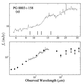
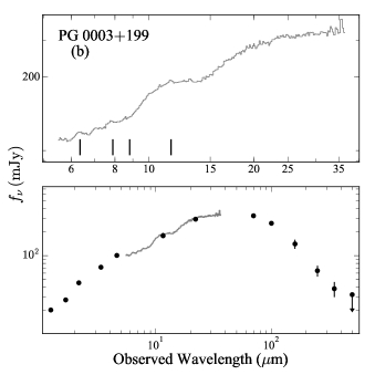
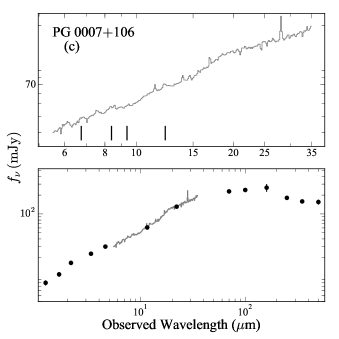
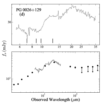
Figure 1: IR SEDs of four representative PG quasars. For each object, the upper panel shows the details of the IRS spectra from $\sim$ 5 to 40 µm (gray), and the lower panel shows the full SED from $\sim$ 1 to 500 µm. The black vertical lines in the upper panel highlights the location of the most prominent PAH features at 6.2, 7.7, 8.6, and 11.3 µm. The SEDs of the entire sample (87 images) can be found in the online version.

4 SED Fitting Methods

4.1 SED Models

Table 5: Model Parameters and Priors

Model	Parameter	Units	Discreteness	Prior
(1)	(2)	(3)	(4)	(5)
BC03	$M_{*}$	$M_{\odot}$	✘	[$10^{6}$, $10^{14}$]
	$t$	Gyr	✔	5 (fixed)
BB	$\Omega_{\mathrm{dust}}$	Sr	✘	[$10^{-25}$, $10^{-10}$]
	$T$	K	✘	[500, 1500]
CLUMPY	$i$	–	✔	[0.0, 90.0]
	$\tau_{V}$	–	✔	[10.0, 300.0]
	$q$	–	✔	[0.0, 3.0]
	$N_{0}$	–	✔	[1.0, 15.0]
	$\sigma$	–	✔	[15.0, 70.0]
	$Y$	–	✔	[5.0, 100.0]
	$L$	erg s-1	✘	[$10^{40}$, $10^{50}$]
DL07	$U_{\mathrm{min}}$	–	✔	[0.10, 25.0]
	$U_{\mathrm{max}}$	–	✔	$10^{6}$ (fixed)
	$\alpha$	–	✘	2 (fixed)
	$q_{\mathrm{PAH}}$	–	✔	[0.3, 4.8]
	$\gamma$	–	✘	[0.0, 1.0]
	$M_{d}$	$M_{\odot}$	✘	[$10^{6}$, $10^{\mathrm{11}}$]
Synchrotron	$\alpha$	–	✘	[0.0, 5.0]
	$f_{0}$	–	✘	[$10^{-5}$, $10^{5}$]

The IR SED consists of emission from various physical sources inside a galaxy. The stellar emission usually mainly contributes to the NIR, the bands covered by 2MASS. The emission from the AGN dust torus dominates the quasar SED up to $\sim 30$ µm, covered by WISE and IRS. At longer wavelengths, in the regime of the Herschel bands, dust emission from the galactic-scale ISM becomes brighter than the torus emission. If the quasar is radio-loud, the jet contributes strong synchrotron radiation, which usually dominates the GHz radio bands but may extend to and sometimes even dominate the submillimeter regime. Since the emission from all of these physical components overlap, we must fit the entire IR SED by simultaneously modeling all of the emission components, in order to get an unbiased measurement of the host galaxy dust properties. The models we consider and their associated parameters are summarized in Table 5. The following describes them in detail.

The stellar emission is represented by a simple stellar population model from Bruzual & Charlot (2003, hereafter BC03) with a Chabrier (2003) stellar IMF. We use the Python package EzGal (Mancone & Gonzalez, 2012) to generate the template spectra. The stellar age is, in principle, a free parameter, but we fix it to 5 Gyr because we can hardly solve for the stellar age independently without additional constraints on the stellar emission of the host galaxy in the optical bands. This, however, is extremely challenging because of the dominance of AGN emission at shorter wavelengths. Moreover, the spectral shape of the NIR stellar emission is governed mostly by the old stellar population, rendering it relatively insensitive to stellar age. Therefore, fixing the stellar age of the BC03 template is expected to have a negligible effect on the derived dust properties.

For the dust torus emission, we incorporate the templates generated by the radiative transfer model CLUMPY (Nenkova et al., 2008a, b). We also test two other dust torus radiative transfer models provided by Hönig & Kishimoto (2010) and Siebenmorgen et al. (2015). For all three models, in order to get a good fit to the MIR data, an additional hot ($T\approx 1000$ K) blackbody (BB) component is required (Deo et al., 2011; Mor & Netzer, 2012). This is likely because these models all assume that silicate and carbon dust have the same temperature distributions (R. Siebenmorgan 2017, private communication). However, in reality, carbonaceous dust can have higher temperature, such that the real dust torus displays excess emission at wavelengths $\lesssim 5$ µm (García-González et al., 2017; Hönig & Kishimoto, 2017). A detailed analysis of how different dust torus templates fit quasar SEDs and how they affect the cold dust measurements is beyond the scope of the current work. Nevertheless, we do worry whether the choice of torus model may introduce model-dependent systematic uncertainties in our fitting. In Appendix C, we demonstrate that the torus model does not bias the key derived cold dust parameters—especially the dust mass—as long as the FIR data constrain well the peak and the Rayleigh-Jeans tail of the dust emission. One of the advantages of the CLUMPY model is that there are $\sim$ $10^{6}$ templates available, more than two orders of magnitude larger than the other two sets of models. The higher the density of the sampled parameter grids, the more robust the model we can reconstruct by interpolating the model templates (see Appendix D.1). The CLUMPY model has seven free parameters: the optical depth of the individual cloud $\tau_{V}$, the power-law index $q$ of the cloud radial distribution, the ratio $Y$ of outer and inner radii of the dust torus, the average number of clouds on the equatorial ray $N_{0}$, the standard deviation $\sigma$ of the Gaussian distribution of the number of clouds in the polar direction, the observer’s viewing angle $i$ from the torus axis, and the luminosity $L$ normalization factor. The complementary BB component,

$$f_{\mathrm{\nu,BB}}=\Omega_{d}\,B_{\nu}(T),$$ (1)

has two free parameters, $\Omega_{d}$ the solid angle subtended by the dust and $B_{\nu}(T)$ the Planck function with temperature $T$. Hence, the CLUMPY+BB model has a total of nine parameters.

The galactic dust emission is described by the widely used DL07 model. The model is based on the dust composition and size distribution observed in the Milky Way (MW). The dust emission templates are calculated including the single-photon heating process, which produces the PAH features. The radiation intensity relative to the local interstellar radiation field is parametrized by $U$. The DL07 model assumes that most of the dust in a galaxy is located in the “diffuse ISM” and exposed to the radiation field with the same intensity $U=U_{\mathrm{min}}$, the minimum radiation field intensity of the galaxy. A small fraction ($\gamma$) of dust is heated by photons from a power-law distribution of $U$, with $U_{\mathrm{min}}<U<U_{\mathrm{max}}$ ($U_{\mathrm{min}}\ll U_{\mathrm{max}}$), referred to as the “photodissociation region” component for normal galaxies, since the wide range of $U$ may come from photodissociation regions related to massive stars. The dust grains are a mixture of amorphous silicate and graphite, including PAH particles with mass fraction $q_{\mathrm{PAH}}$. The rest-frame flux density of the DL07 model is

$$f_{\mathrm{\nu,\,DL07}}=\frac{M_{d}(1+z)^{2}}{4\pi D_{L}^{2}}[(1-\gamma)p_{\nu}^{(0)}(q_{\mathrm{PAH}},\,U_{\mathrm{min}})+\gamma p_{\nu}(q_{\mathrm{PAH}},\,U_{\mathrm{min}},\,U_{\mathrm{max}},\,\alpha)],$$ (2)

where $M_{d}$ is the dust mass, $z$ is the redshift, $D_{L}$ is the luminosity distance, and $p_{\nu}^{(0)}(q_{\mathrm{PAH}},\,U)$ is the power radiated per unit frequency per unit mass of the dust mixture determined by $q_{\mathrm{PAH}}$ exposed to the radiation field with intensity $U$. The specific power of unit dust mass is

$$p_{\nu}(q_{\mathrm{PAH}},\,U_{\mathrm{min}},\,U_{\mathrm{max}},\,\alpha)=\frac{(\alpha-1)}{U_{\mathrm{min}}^{1-\alpha}-U_{\mathrm{max}}^{1-\alpha}}\,\int_{U_{\mathrm{min}}}^{U_{\mathrm{max}}}p_{\nu}^{(0)}(q_{\mathrm{PAH}},\,U)\,U^{-\alpha}\,dU,$$ (3)

where $\alpha$ is the power-law index of the interstellar radiation field intensity distribution. DL07 provide the precalculated $p_{\nu}^{(0)}(q_{\mathrm{PAH}},\,U_{\mathrm{min}})$ and $p_{\nu}(q_{\mathrm{PAH}},\,U_{\mathrm{min}},\,U_{\mathrm{max}},\,\alpha)$ as model templates. By studying the SEDs of normal star-forming galaxies, Draine et al. (2007) found that, for all situations, we can fix $\alpha=2$ and $U_{\mathrm{max}}=10^{6}$. We adopt this simplification, assuming that quasar host galaxies have a distribution of radiation field intensity similar to that of typical star-forming galaxies. Therefore, the DL07 model contains four free parameters: $q_{\mathrm{PAH}}$ and $U_{\mathrm{min}}$ are discrete, and $\gamma$ and $M_{d}$ are continuous.

The radio-loud objects are defined by the radio-loudness parameter, $R\equiv f_{\nu}({\rm 6~{}cm})/f_{\nu}$(4400 Å), such that $R\geq 10$ (Kellermann et al., 1989). The synchrotron radiation of radio-loud objects may contaminate considerably the dust thermal emission in the submillimeter. To fit the synchrotron component, we adopt a broken power-law model (e.g., Pe’er 2014)

$$f_{\nu,\mathrm{syn}}\propto\begin{cases}\nu^{-\alpha}&\nu<\nu_{\mathrm{c}},\\ \nu^{-\alpha-1/2}&\nu_{\mathrm{c}}<\nu<\nu_{\mathrm{max}},\\ 0&\nu>\nu_{\mathrm{max}},\end{cases}$$ (4)

where $\nu_{c}=10^{13}$ Hz is the cooling frequency, above which the power-law slope becomes steeper, and we assume that the highest frequency of the synchrotron emission is $\nu_{\mathrm{max}}=10^{14}$ Hz. The typical power-law slope for steep-spectrum quasars is $\alpha\approx 0.7$, and we can use the radio SED to anchor the synchrotron component. For flat-spectrum quasars (Urry & Padovani, 1995) whose radio emission varies greatly, the archival radio data, taken at different times, cannot be fitted by the synchrotron radiation model. Nevertheless, we find that, with the help of submillimeter data, it is possible to fit three flat-spectrum quasars in our sample (PG 0007$+$106, PG 1226$+$023, and PG 1302$-$102) with reasonable power-law slopes ($\alpha\approx$ 0.7–1.3). In the remaining two objects (PG 1309$+$355 and PG 2209$+$184), the synchrotron emission is not dominant, and so it will only marginally affect, if at all, the global fit. The $f_{0}$ in Table 5 is the scaling factor of the synchrotron model.

The final model SED is the linear combination of the BC03, BB, CLUMPY, DL07, and, if necessary, the synchrotron components. To directly compare with the observed photometric data, we need to fold the model SED through the response functions of the respective photometric bands (Bessell & Murphy, 2012). For the 2MASS and WISE bands, our quoted flux density is the band-averaged flux density,

$$\langle f_{\nu}\rangle=\frac{\int f_{\nu}(\nu)S(\nu)d\nu/\nu}{\int S(\nu)d\nu/\nu},$$ (5)

where $S(\nu)$ is the system photon response function. In the case of the Herschel bands, the data are monochromatic flux densities at the nominal frequency $\nu_{0}$,

$$f_{\nu_{0}}=\frac{1}{\nu_{0}}\frac{\int S^{\prime}(\nu)d\nu}{\int S^{\prime}(\nu)d\nu/\nu}\langle f_{\nu}\rangle,$$ (6)

where $S^{\prime}(\nu)$ is the system energy response function, and the band-averaged flux density becomes (Section 5.2.4 of SPIRE handbook)

$$\langle f_{\nu}\rangle=\frac{\int f_{\nu}(\nu)S^{\prime}(\nu)d\nu}{\int S^{\prime}(\nu)d\nu}.$$ (7)

No additional reprocessing is necessary to mimic the observations of Spitzer because the PAH features in DL07 are already designed to match the low-resolution IRS spectra.

4.2 Fitting Method

In order to simultaneously fit the photometric and spectroscopic data, we develop a Bayesian MCMC fitting algorithm. The code can incorporate an arbitrary number of models to obtain a combined SED model. The Bayesian method (Gregory 2005) implies that the posterior probability density function (PDF) of model parameters, $\Theta=[\theta_{1},\theta_{2},...]$, given the prior knowledge $I$ and data $D$, is

$$p(\Theta|D,I)=\frac{p(\Theta|I)p(D|\Theta,I)}{p(D|I)}.$$ (8)

The prior, $p(\Theta|I)$, is provided by our prior knowledge about the probability distribution of the model parameters. The evidence, $p(D|I)$, is a normalization factor that does not affect the fitting with a given model. It may be important when we need to compare different models, but this is beyond the scope of the current work, and we do not consider it further.

The likelihood of the data, $\mathscr{L}=p(D|\Theta,I)$, being observed with the given prior knowledge and model parameters is assumed to be

$$\mathrm{ln}\,\mathscr{L}=\mathrm{ln}\,\mathscr{L}_{p,d}+\mathrm{ln}\,\mathscr{L}_{p,u}+\mathrm{ln}\,\mathscr{L}_{s},$$ (9)

where $\mathrm{ln}\,\mathscr{L}_{p,d}$ and $\mathrm{ln}\,\mathscr{L}_{p,u}$ are the ln-likelihoods of the photometric data with detection and upper limits, respectively, while $\mathrm{ln}\,\mathscr{L}_{s}$ is the ln-likelihood of the spectra. We adopt

$$\mathrm{ln}\,\mathscr{L}_{p,d}=-\frac{1}{2}\left(\sum_{i}^{n}\,\frac{(y_{i}-\tilde{y}_{i}(\Theta))^{2}}{s_{i}^{2}}+\sum_{i}^{n}\mathrm{ln}\,(2\pi s_{i}^{2})\right),$$ (10)

$$\mathrm{ln}\,\mathscr{L}_{p,u}=\sum_{j}^{m}\,\mathrm{ln}\,\frac{1+\mathrm{erf}(z_{j})}{2},~{}z_{i}=\frac{y_{i}-\tilde{y}_{i}(\Theta)}{\sqrt{2}s_{i}},$$ (11)

with

$$s_{i}^{2}=\sigma_{i}^{2}+(f\tilde{y}_{i}(\Theta))^{2},$$

where $y_{i}$ and $\tilde{y}_{i}$ are the observed and model synthetic flux densities, $\mathrm{erf}(x)$ is the error function, and $\sigma_{i}$ is the observational uncertainty, three times which is considered to be the upper limit. We introduce a parameter $f$ into $s_{i}$, the square root of the inverse weight, to consider the systematic uncertainty from the model to the real data. In order to balance the weight of the data at different wavelengths, some works assign a 10% additional uncertainty to all of the bands (e.g., Draine et al. 2007). Others choose to use a uniform weight for all of the bands instead of incorporating the observational uncertainty. Our approach, by contrast, assumes the typical percentage for the model to deviate from the data to be $f$ and lets the MCMC algorithm fit for $f$ as a free parameter. This method to consider upper limits for the data has been widely used (e.g., Isobe et al. 1986; Lyu et al. 2016; Shimizu et al. 2017). For spectroscopic data, the residual between data and model may be highly correlated (Czekala et al., 2015), and so we need to model the residual correlation. For the spectra, we adopt

$$\mathrm{ln}\,\mathscr{L}_{s} = -\frac{1}{2}\left(\textbf{r}^{T}\,\textbf{K}^{-1}\,\textbf{r}+\mathrm{ln}\,\det{\textbf{K}}+N\,\mathrm{ln}\,2\pi\right),$$ (12)

$$K_{i,j} = s_{i}^{2}\,\delta_{i,j}+k_{i,j},$$

$$k_{i,j} = a^{2}\left(1+\frac{\sqrt{3}|\lambda_{i}-\lambda_{j}|}{\tau}\right)\exp{\left(-\frac{\sqrt{3}|\lambda_{i}-\lambda_{j}|}{\tau}\right)},$$ (13)

where $r_{i}=y_{i}-\tilde{y}_{i}(\Theta)$ is the residual between data and model, K is the covariance matrix, $N$ is the length of the data, $\delta_{i,j}$ is the Kronecker delta, and $k_{i,j}$ describes the correlation between two residuals at wavelengths $\lambda_{i}$ and $\lambda_{j}$. We choose $k_{i,j}$ to be the Matérn $3/2$ function (Rasmussen & Williams, 2016), where $a$ is the strength of the correlation and $\tau$ is the characteristic length of the correlation. There are, in total, three free parameters ($f$, $a$, and $\tau$) that enter the fitting to model the uncertainties. We use the Python package George (Ambikasaran et al., 2014) to calculate the matrix inverse and determinant with Gaussian process regression method. With more realistic treatments of the uncertainties and residuals, our likelihood function is flexible enough to balance the weight of the photometric and spectroscopic data in the fitting.

Due to the complexity of the model (up to 19 parameters to be fitted), we have to rely on the MCMC method to sample the parameter space. We develop a Python code to construct the model and use the package emcee (Foreman-Mackey et al., 2013) to sample the posterior PDF (see Appendix D.1 for details). In order to ascertain whether the Bayesian MCMC fitting method can effectively constrain the model parameters, we generate mock SEDs with the best-fit models of the quasar SEDs and their realistic uncertainties and upper limits. The details of the test are described in Appendix D.2. We find that the DL07 parameters can be reliably measured with our fitting strategy. The scatter of the input and best-fit dust masses is 0.16 dex for the entire sample, with no systematic deviation. For the 44 objects whose FIR SEDs are good enough to cover the peak and Rayleigh-Jeans tail of the dust emission, the scatter of the dust mass is only 0.09 dex. $U_{\mathrm{min}}$ and $q_{\mathrm{PAH}}$ are discrete parameters. Their best-fit results are typically $\lesssim 2$ grid points away from the input values, except for some objects with very poor detections in the FIR. The $\gamma$ parameter controls the amount of dust emission from the power-law part of the radiation field, which mainly contributes in the MIR, overlapping with the AGN torus emission. Therefore, $\gamma$ is mostly affected by the AGN torus model. The fitting results may be unreliable for objects with $\gamma\lesssim 0.01$.

5 Results

5.1 SED Fitting

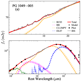
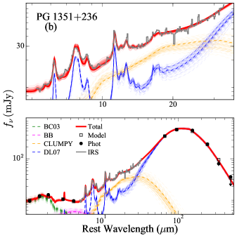
Figure 2: Best-fit results for (a) PG 1049$-$005 and (b) PG 1351$+$236. The lower panels show the entire IR SEDs while the upper panels zoom in to display the details of the IRS spectrum covering $\sim$ 5 to 40 µm (gray line). The black points are the photometric data from 2MASS, WISE, and Herschel. The dashed lines are the best-fit models: BC03 (green), BB hot dust (magenta), CLUMPY torus (orange), and DL07 (blue). The combined total model is the red solid line. To visualize the model uncertainties, the associated thin lines in light color represent 100 sets of models with parameters drawn randomly from the space sampled by the MCMC algorithm. With detections in four Herschel bands, PG 1049$-$005 can already provide good constraints on the model. In the case of PG 1351$+$236, which has prominent PAH features, the best-fit model captures the features of the SED on both large and small scales. The best-fit results of the entire sample (87 images) can be found in the online version.

Best-fit results are shown in Figure 2 for two objects with Herschel detections in four or more bands. The best fit and each component of the models are displayed with dashed lines in different colors. To illustrate the uncertainty of the model (components), we randomly choose 100 sets of parameters from the MCMC-sampled parameter space and plot them with light thin lines. The lower panels show the full SED and the best-fit models while the upper panels zoom in to display the details of the spectra in the range 5–40 µm. The best-fit model not only matches the large-scale structure of the SED but also properly captures the detailed PAH features of the spectra.

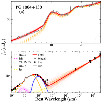
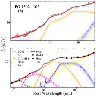
Figure 3: Best-fit results for (a) the steep-spectrum quasar PG 1004$+$130 and (b) the flat-spectrum quasar PG 1302$-$102. The symbols are the same as in Figure 2. The synchrotron emission (yellow) is negligible at FIR wavelengths for PG 1004+130, whereas it is dominant in PG 1302$-$102, although its radio emission varies too much to be used to constrain the synchrotron model.

Figure 3 shows the fitting results for two radio-loud objects. PG 1004$+$130 is a steep-spectrum radio quasar. The synchrotron emission (yellow), anchored by radio data collected from the archives, contributes negligibly at FIR wavelengths. As a flat-spectrum radio quasar, PG 1302$-$102 exhibits too much radio variability to constrain the synchrotron model, and we resort to fitting the IR SED without additional radio data. Even though the synchrotron emission is very strong, all of the dust components are reasonably well constrained. The power-law slope is $\sim$ 0.8. The DL07 component is not significantly affected by the synchrotron emission for all the radio-loud objects. The only exception is PG 1226+023, whose synchrotron emission is so strong that the cold dust emission is totally overwhelmed; its dust mass is very uncertain, as reflected in its error bar.

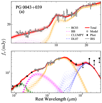
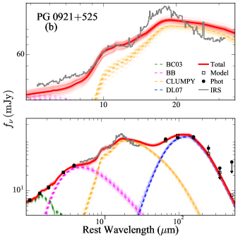
Figure 4: Best-fit results for (a) PG 0043+039 and (b) PG 0921+525. The symbols are the same as in Figure 2. The DL07 model is not well constrained for PG 0043$+$039, mainly because there are only two Herschel bands detected. Nevertheless, the upper limits still provide some useful constraints on the best-fit model, albeit with larger uncertainties. The spectrum of PG 0921$+$525 is not well fit by the CLUMPY model, which likely cannot account for the different dust composition in this object. However, this mismatch will barely affect the measurement of the dust mass (Appendix C).

Still, not all fits are reliable. This applies primarily to some distant (fainter) objects that are not well detected by Herschel. As illustrated by PG 0043$+$039 (Figure 4(a)), the DL07 model cannot be well constrained. However, this only happens when there is no detected Herschel band where the DL07 model contributes non-negligible emission. We visually check all of the fitting results and find 11 objects whose DL07 model cannot be well constrained by the FIR SED. If we allow the DL07 parameters to be free, the model adjusts to mainly fit the mismatch between the data and the CLUMPY component. Under these circumstances, we simply attempt to place an upper limit on the allowed dust mass. We fix the dust mass in the fit, manually and iteratively adjusting $M_{d}$ in increments of 0.1 dex. Meanwhile, $M_{d}$ is degenerate with $U_{\mathrm{min}}$: lower values of $U_{\mathrm{min}}$ lead to higher $M_{d}$. For the purposes of obtaining a robust, conservative upper limit on $M_{d}$, we fix $U_{\mathrm{min}}=1.0$ since the diffuse radiation field of quasar host galaxies is not likely weaker than that of the solar neighborhood. In normal, star-forming galaxies, $U_{\mathrm{min}}$ hardly ever reaches below 1 (Draine et al., 2007). We also fix $q_{\mathrm{PAH}}=0.47$, the minimum value of the model grid, although in practice the actual value of $q_{\mathrm{PAH}}$ makes little difference because the DL07 component of the 11 objects is always negligible at MIR wavelengths compared to the torus component.

Another complication arises when the CLUMPY component cannot fit the IRS spectrum well (Figure 4(b)), presumably because the dust torus of some objects has an unusual chemical composition (Xie et al., 2017, hereafter, XLH17) that differs from that assumed in the standard CLUMPY model. In these situations, we usually need to limit the amplitude of the covariance ($a$), so that the template is forced to match the spectrum, regardless of the detailed features. This may introduce systematic errors to the DL07 model. This issue is addressed in Appendix C, where we investigate the impact on the DL07 parameters by replacing the CLUMPY model with the optically thin dust emission model proposed by XLH17. We find that both torus models yield consistent values of $U_{\mathrm{min}}$ and $M_{d}$, especially for the objects with good FIR data. The $\gamma$ parameter shows some systematic discrepancies, but this is expected because it is mostly degenerate with the torus model. The scatter in $q_{\mathrm{PAH}}$ is large, likely because, for some cases, the XLH17 model poorly matches the spectra below $\sim$ 10 µm (see Appendix C for details).

Furthermore, as we later show (Section 6.2), the modified blackbody (MBB) model, when properly used, can provide dust masses that are quite consistent with those derived with the DL07 model from full SED fitting. In summary: our measurements of dust masses in quasar host galaxies from the DL07 model and full SED fitting are not likely biased compared to those of normal galaxies.

5.2 ISM Radiation Field: Evidence for AGN Heating of Dust

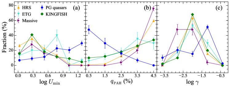
Figure 5: Distribution of DL07 parameters (a) $U_{\mathrm{min}}$, (b) $q_{\mathrm{PAH}}$, and (c) $\gamma$ for PG quasars (blue circles) and star-forming galaxies from the KINGFISH (green diamonds) and HRS (upward orange triangles) samples. Two subsamples of HRS galaxies are plotted. The downward cyan triangles are early-type galaxies (S0 and elliptical, according to Boselli et al. 2010; 17 objects), while the rightward purple triangles are massive galaxies with stellar mass $>10^{10.5}\,M_{\odot}$ (25 objects). The uncertainties for PG quasars and HRS galaxies are estimated with a Monte Carlo method, resampling the parameters according to their measured uncertainties and calculating the number of galaxies in each bin for 500 times. The local star-forming and quenched galaxies in the KINGFISH and HRS samples peak at low $U_{\mathrm{min}}$ but high $q_{\mathrm{PAH}}$. By contrast, PG quasar host galaxies tend to have higher $U_{\mathrm{min}}$ and lower $q_{\mathrm{PAH}}$. The early-type galaxies tend to have higher $U_{\mathrm{min}}$ but mainly peak at intermediate values, $U_{\mathrm{min}}<10$.

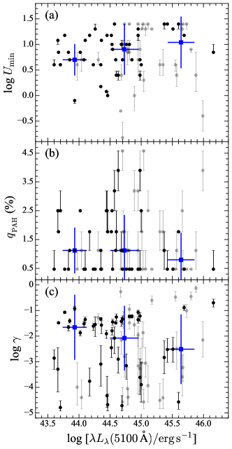
Figure 6: Relation between AGN optical luminosity and DL07 parameters (a) $U_{\mathrm{min}}$, (b) $q_{\mathrm{PAH}}$, and (c) $\gamma$. The dark points represent more robust fitting results than the gray points; we omitted objects for which only upper limits are available for the dust mass. The sample is binned according to $\mathrm{log}\,[\lambda L_{\lambda}$(5100 Å)/$\mathrm{erg\,s^{-1}}]$: $<44.25$, 44.25–45.25, and $\geq 45.25$; the median and standard deviation of the parameter values in each bin are plotted as blue squares with error bars. Since $U_{\mathrm{min}}$ and $q_{\mathrm{PAH}}$ are discrete parameters, their errors may not be resolvable if they are smaller than the size of the grid.

Our approach to SED fitting using the DL07 model allows us to diagnose some important properties of the ISM, namely the strength of the “diffuse” radiation field ($U_{\mathrm{min}}$), the mass fraction of warm dust ($\gamma$), and the mass fraction of the dust contained in PAHs ($q_{\mathrm{PAH}}$). Although the best-fit parameters for individual objects may have relatively large uncertainties, the distribution of parameters for the sample may yield insights into the ensemble properties of quasar host galaxies. Figure 5 compares the distributions of $U_{\mathrm{min}}$, $q_{\mathrm{PAH}}$, and $\gamma$ for the PG quasars in relation to the sample of normal galaxies from KINGFISH and HRS. The distributions of the three parameters for the KINGFISH and HRS galaxies are very similar, even though the KINGFISH sample comprises essentially gas rich, star-forming galaxies while more than half of the HRS galaxies are gas poor (Ciesla et al., 2014). The uncertainties for PG quasars and HRS galaxies are estimated with a Monte Carlo method, resampling the parameters according to their measured uncertainties and calculating the number of galaxies in each bin for 500 times.

Relative to the normal galaxies, the quasar hosts display a higher fraction of $U_{\mathrm{min}}$ at high values. A higher $U_{\mathrm{min}}$ signifies a stronger ISM radiation field. What is the source of this enhancement? One possibility is that quasar host galaxies may have stronger star formation activity than normal galaxies. Quasar host galaxies may have experienced a recent starburst, whose magnitude scales with the AGN luminosity (Kauffmann et al., 2003). This interpretation, however, is not supported by the evidence in hand. Based on the strength of the 11.3 $\mu$m PAH feature, Zhang et al. (2016) find that PG quasars have similar star formation rates to “main-sequence” star-forming galaxies of similar stellar mass. Husemann et al. (2014) come to the same conclusion, for another quasar sample. Our own analysis indicates that quasar hosts, in fact, have lower values of $q_{\mathrm{PAH}}$ compared with normal galaxies (Figure 5(b)). In conjunction with the mild reduction of $q_{\mathrm{PAH}}$ with increasing AGN luminosity (Figure 6(b)), this supports the idea that PAHs tend to be destroyed by the high-energy photons from the AGN (Smith et al., 2007; Sales et al., 2010; Wu et al., 2010). It is unlikely that the reduction of PAH strength stems from enhanced MIR extinction, as we find no clear evidence for dust absorption features in the IRS spectra. In this work, we will not attempt to resolve the inherent ambiguity on the interpretation of the reduced strength of PAH features in PG quasars (i.e. intrinsic reduction in star formation rate or AGN destruction of PAHs). Suffice it to say, there is no compelling evidence that the star formation rate is enhanced in our sample of PG quasars. In support of this conclusion, we note that among the six objects with the highest values of $U_{\mathrm{min}}$ and optical AGN luminosity [$\mathrm{log}\,U_{\mathrm{min}}>1.2$ and $\lambda L_{\lambda}$(5100 Å) $>10^{45}\,\mathrm{ergs^{-1}}$], three (PG 1004$+$130, PG 1116$+$215, and PG 1416$-$129) have host galaxies that resemble giant elliptical galaxies in HST images (Y. Zhao et al. 2018, in preparation). Furthermore, PG 1416$-$129 is found to be gas poor (Section 5.3). Alternatively, perhaps $U_{\mathrm{min}}$ is enhanced by old stars. An evolved stellar population or enhanced stellar surface density may drive the radiation field to a very high intensity level (e.g., Mentuch Cooper et al. 2012), although Rowlands et al. (2015) find that the cold dust temperature for a small sample of post-starburst galaxies is not unusually high compared to normal star-forming galaxies. In Figure 5, we also plot two subsamples of HRS galaxies, with early-type galaxy morphology and with stellar masses $>10^{10.5}\,M_{\odot}$. The values of $U_{\mathrm{min}}$ of early-type galaxies, dominated by an old stellar population, tend to be higher than those of other galaxy samples but are not as high as in quasar host galaxies.

If the elevated radiation intensity of quasar hosts is not due to an excess of young or old stars, it is likely that the ISM is heated, at least in part, by the central AGN. From the spatial extent of the narrow-line region (Greene et al., 2011; Husemann et al., 2014), we know that the radiation field of the AGN can reach large distances into the host galaxy. As the narrow-line region gas is dusty (e.g., Kraemer et al. 2011; Wild et al. 2011), it is natural for the associated dust to experience enhanced heating from the AGN. Studies of the MIR spectra of quasars also reveal that AGN-heated silicate emission likely comes from the narrow-line region (Schweitzer et al., 2008; Mor et al., 2009). Figure 6(a) shows that $U_{\mathrm{min}}$ increases with increasing AGN luminosity, although the scatter is relatively large for individual objects. We note that the distribution of $\gamma$ (Figures 5(c)) further supports the notion that the dust in the host galaxies of quasars is exposed to a higher intensity radiation field than star-forming galaxies, while the scatter in Figure 6(c) is large (see Appendix D.2 for caveats on the interpretation of $\gamma$).

The ability for the AGN or any sources other than young stars to heat dust appreciably on galactic scale raises serious doubt for the common practice of using the FIR luminosity to estimate star formation rates in AGN host galaxies (e.g., Leipski et al. 2014; Podigachoski et al. 2015; Westhues et al. 2016; Shimizu et al. 2017). Our results suggest that attempts to remove the dust torus contribution alone from the IR SED may not be enough to guarantee that the FIR luminosity is uncontaminated by AGN emission.

5.3 ISM Mass

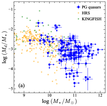
Figure 7: (a) Dust-to-stellar mass ratio is plotted against the stellar mass of PG quasars (blue) and inactive nearby galaxies from HRS (orange; $M_{*}$: Boselli et al. 2010, Cortese et al. 2012; $M_{d}$: Ciesla et al. 2014) and KINGFISH (green; $M_{*}$: Kennicutt et al. 2011, Skibba et al. 2011; $M_{d}$: Draine et al. 2007). (b) Gas-to-stellar mass ratio is plotted against the stellar mass of PG quasars (blue) and inactive nearby galaxies from HRS (orange; $M_{\mathrm{gas}}$: Boselli et al. 2014a) and COLD GASS (green; Saintonge et al. 2012). The typical uncertainty of the PG sample is shown in the lower-left corner. Total stellar masses for the PG quasars come from Zhang et al. (2016); lower limits on $M_{*}$ (and upper limits on $M_{d}/M_{*}$ and $M_{\rm gas}/M_{*}$; denoted with downward and rightward arrows) come from bulge masses estimated from the $M_{\mathrm{BH}}$–$M_{\mathrm{bulge}}$ relation. Objects that only have upper limits on the dust masses are also included.

5.3.1 Dust Mass

One of the main goals of this study is to apply the DL07 model to our SED fitting to measure dust masses for the PG quasars. We derive dust masses in the range $M_{d}\approx 10^{6.2}-10^{8.7}\,M_{\odot}$ (Table 1), with a mean value of $10^{7.6\pm 0.1}\,M_{\odot}$, properly accounting for upper limits using the Kaplan–Meier product-limit estimator KMESTM from ASURV (Feigelson & Nelson, 1985; Lavalley et al., 1992).

Figure 7(a) plots the distribution of dust-to-stellar mass ratio as a function of stellar mass for PG quasars, comparing them with normal galaxies from the HRS and KINGFISH samples. As expected, the quasar hosts are all massive galaxies ($M_{*}\gtrsim 10^{10}\,M_{\odot}$), with the majority lying in a relatively narrow range of $M_{*}\approx 10^{11.0\pm 0.5}\,M_{\odot}$. The dust-to-stellar mass ratio of PG quasars follows the general trend and dispersion ($\sim 2$ dex) of normal galaxies. For the objects with very low $M_{d}/M_{*}$ (e.g., $\lesssim 10^{-4}$), we visually check the fitting to confirm their robustness. Among these objects, four (PG 0804$+$761, PG 1416$-$129, PG 1501$+$106, and PG 1534$+$580) have highly secure dust masses because the detected FIR data cover the Rayleigh-Jeans tail of the SED. In another four (PG 0026$+$129, PG 0049$+$171, PG 0923$+$201, and PG 2304$+$042), the peak of the DL07 model can be barely constrained, but, as shown in Appendix D.2, the error on the dust mass for an individual object can hardly exceed 0.3 dex, and hence these objects are still deficient in dust compared to the majority of the sample. The dust mass for PG 1226$+$023 is very uncertain because the emission from its torus and synchrotron components are very strong. Another source of uncertainty comes from the host galaxy stellar mass or the bulge mass estimated from $M_{\mathrm{BH}}$, but it is unlikely that $M_{*}$ has been overestimated by more than 0.3 dex for these objects. The quoted uncertainty of the stellar mass is $\sim 0.2$ dex (Zhang et al., 2016), while the intrinsic scatter of the $M_{\mathrm{BH}}$–$M_{\mathrm{bulge}}$ relation is $\lesssim 0.3$ dex.

5.3.2 Gas Mass

The dust and total gas masses are linked by

$$M_{\mathrm{gas}}=M_{\mathrm{H\,I}}+M_{\mathrm{H_{2}}}=M_{d}\,\delta_{\mathrm{GDR}},$$ (14)

where $\delta_{\mathrm{GDR}}$ is the gas-to-dust ratio, which is a function of the gas-phase metallicity (Boselli et al., 2002; Draine et al., 2007; Leroy et al., 2011; Magdis et al., 2012). Assuming that the same fraction of condensable elements is locked in dust as in the MW, and that the interstellar abundance of carbon and all of the heavier elements are proportional to the gas-phase oxygen abundance, Draine et al. (2007) suggest $\delta_{\mathrm{GDR}}=136[\mathrm{(O/H)_{MW}}/\mathrm{(O/H)]}$, where $\mathrm{(O/H)_{MW}}$ is the oxygen abundance in the local MW and the factor of 136 is from MW dust models (Draine et al., 2007), including helium and heavier elements. Leroy et al. (2011) simultaneously constrain $\alpha_{\mathrm{CO}}$ and $\delta_{\mathrm{GDR}}$ with spatially matched dust, CO, and H I maps of some local group galaxies. They find a clear dependence of $\delta_{\mathrm{GDR}}$ on the gas-phase metallicity ($\delta_{\mathrm{GDR}}$–$Z$ relation), consistent with theoretical expectation (Draine et al., 2007). Magdis et al. (2012) recalibrate the $\delta_{\mathrm{GDR}}$–$Z$ relation of Leroy et al. (2011) to the empirical calibration of Pettini & Pagel (2004, hereafter, PP04), as follows,

$$\mathrm{log}\,\delta_{\mathrm{GDR}}=(10.54\pm 1.0)-(0.99\pm 0.12)[12+\mathrm{log\,(O/H)}]_{\mathrm{PP04}},$$ (15)

where the scatter is 0.15 dex. In the absence of a direct measurement of the metallicity of the galaxy, it can be estimated from the stellar mass–metallicity ($M_{*}$–$Z$) relation (e.g., Magdis et al. 2012; Santini et al. 2014; Berta et al. 2016), if the stellar mass is known. Since our focus is on low-redshift objects, we adopt the $M_{*}$–$Z$ relation obtained for SDSS galaxies with the PP04 (N2) calibration, as given by Kewley & Ellison (2008),

$$12+\mathrm{log\,(O/H)}=23.9049-5.62784\,\mathrm{log}\,M_{*}+0.645142\,(\mathrm{log}\,M_{*})^{2}-0.0235065\,(\mathrm{log}\,M_{*})^{3},$$ (16)

with residual scatter 0.09 dex. As stressed by Berta et al. (2016), it is important to use the $\delta_{\mathrm{GDR}}$–$Z$ and $M_{*}$–$Z$ relations self-consistently in terms of the metallicity calibration. The different calibrations can lead to a significant systematic discrepancy for the $M_{*}$–$Z$ relation in terms of both its shape and scale (see Kewley & Ellison 2008 for detailed discussions). For example, the $M_{*}$–$Z$ relation obtained by Tremonti et al. (2004) from theoretical calibration is $\gtrsim 0.4$ dex higher than the PP04 empirical calibration at $M_{*}\approx 10^{11}\,M_{\odot}$, and the $M_{*}$–$Z$ relation drops much steeper toward lower $M_{*}$ with the former calibration than that with the latter one.

A number of recent works use the dust mass to estimate the total gas mass of galaxies, with $\delta_{\mathrm{GDR}}$ estimated from combining the $M_{*}$–$Z$ and $\delta_{\mathrm{GDR}}$–$Z$ relations (Santini et al., 2014; Magdis et al., 2012; Magdis et al., 2017). We should bear in mind, however, that the metallicity provided by the $M_{*}$–$Z$ relation cannot be guaranteed to provide a proper metallicity that leads to an overall correct $\delta_{\mathrm{GDR}}$–$Z$, for two reasons. First, the metallicity of a galaxy generally decreases with increasing distance from the center (Henry & Worthey, 1999). When the overall metallicity is estimated from the $M_{*}$–$Z$ relation, it is likely that the metallicity is overestimated in the sense that the light from the inner part of the galaxy, where the metallicity is high, dominates the observed spectrum. Second, the $\delta_{\mathrm{GDR}}$ from “local” relations (e.g., Equation (15)), can only estimate the gas mass within the region of the galaxy that contains detectable dust emission ($\lesssim 1.5R_{25}$; Ciesla et al. 2012; Dale et al. 2012, 2017). However, the size of the dust disk is usually smaller than that of the H I disk, unless the H I distribution is truncated by environmental effects (Thomas et al., 2004; Cortese et al., 2010, 2012). Smith et al. (2016), in fact, reveal extended dust emission out to $2R_{25}$, combining Herschel maps of 110 HRS galaxies and reaching 10 times higher sensitivity than the map tracing dust to $\sim 1.2R_{25}$. Muñoz-Mateos et al. (2009) also find that the dust-to-gas ratio drops faster than the metallicity gradient toward the outskirts of the galaxy, perhaps a consequence of the detailed physics of the evolution of dust grains (Mattsson & Andersen, 2012). Therefore, the aforementioned method tends to underestimate the total gas mass, mainly by excluding the extended H I gas. This problem becomes critical when one compares the gas mass estimated from dust with that directly measured from CO and H I observations. In order to understand how serious the problem is and provide a correction for $\delta_{\mathrm{GDR}}$, we study the HRS sample, for which 176 galaxies have measurements of dust, CO, and H I.

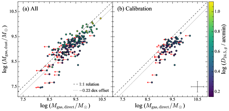
Figure 8: Comparison of gas masses estimated from dust and direct measurements for 176 HRS galaxies having dust, CO, and H I observations. The color code is $D_{24.5,g}$, the diameter of the galaxy at a surface brightness of 24.5 $g$ $\mathrm{mag\,arcsec^{-2}}$. (a) Comparison for the entire sample. The mean deviation (y$-$x) is $-0.09\pm 0.02$ dex; the $50^{+25}_{-25}$th percentile of the deviation is $-0.08^{+0.17}_{-0.19}$ dex. (b) Comparison for the subsample of calibration galaxies with diameters $D_{24.5,g}<3\farcm 5$ and H I deficiency def${}_{\mathrm{H\,I}}<0.5$ (see the text for details). The mean deviation (y$-$x) is $-0.23\pm 0.03$ dex; the $50^{+25}_{-25}$th percentile of the deviation is $-0.22^{+0.18}_{-0.11}$ dex. The statistics are obtained using KMESTM, which accounts for the upper limits. The dashed line is the 1:1 correlation; the dotted line is 0.23 dex below the dashed line, showing the necessary correction to obtain the correct total gas mass. The typical uncertainties of the gas masses are shown in the bottom-right corner.

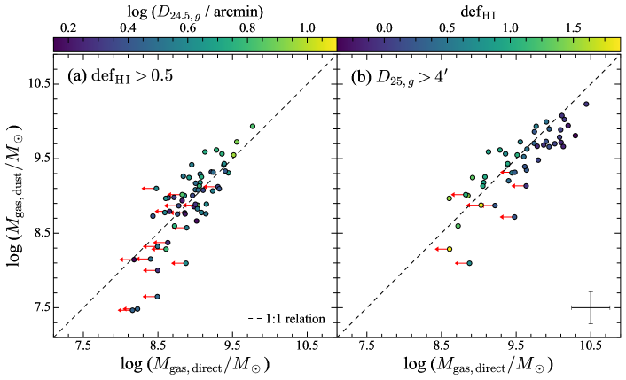
Figure 9: (a) Comparison of total gas masses estimated from dust and direct measurements for H I-deficient HRS galaxies. The color code is $D_{24.5,g}$, the diameter of the galaxy at a surface brightness of 24.5 $g$ $\mathrm{mag\,arcsec^{-2}}$. The dashed line is the 1:1 relation. The mean deviation (y$-$x) is 0.10$\pm$0.03 dex; the $50^{+25}_{-25}$th percentile of the deviation is $0.11^{+0.17}_{-0.15}$ dex. (b) Same comparison, but for the subset of galaxies with $D_{24.5,g}>4\farcm 0$. The color code is the H I deficiency of the galaxy. The mean deviation (y$-$x) is $-0.04\pm 0.04$ dex; the $50^{+25}_{-25}$th percentile of the deviation is $-0.04^{+0.19}_{-0.17}$ dex. The statistics are obtained using KMESTM, which accounts for the upper limits. The typical uncertainties of the gas masses are show in the bottom-right corner.

We find that the total gas mass estimated by dust is on average 0.09$\pm$0.02 dex lower than that obtained from direct measurement, with the $50^{+25}_{-25}$th percentile of the deviation $-0.08^{+0.17}_{-0.19}$ dex (Figure 8(a)). The deviation is apparent but not very significant, because there is a considerable fraction of highly H I-deficient galaxies, whose H I disks are truncated. If we select only the subsample of HRS galaxies with small angular size ($D_{24.5,g}<3\farcm 5$) and low H I deficiency (def${}_{\mathrm{H{\sevenrm\,I}}}<0.5$), the mean deviation is $-0.23\pm 0.03$ dex (dotted line in Figure 8(b)) with the $50^{+25}_{-25}$th percentile $-0.22^{+0.18}_{-0.11}$ dex, which is much more prominent than that for the entire sample.

To ascertain whether $\delta_{\mathrm{GDR}}$ is accurately estimated for HRS galaxies within $\sim R_{25}$ (comparable to the detectable dust emission region), we need to compare dust-derived gas masses to the directly measured gas masses within $\sim R_{25}$. Gas-stripping processes, which truncate the large-scale H I distribution to produce H I-deficient galaxies, provide a natural tool in this regard. Cortese et al. (2010) find that the H I disks of H I-deficient galaxies (def${}_{\mathrm{H{\sevenrm\,I}}}>0.5$) match well the sizes of their dust disks. Figure 9(a) demonstrates that the systematic deviation between the gas masses obtained with the two methods is small for the subset of HRS galaxies classified as H I deficient (def${}_{\mathrm{H{\sevenrm\,I}}}>0.5$). The $50^{+25}_{-25}$th percentile of the gas mass deviation is $0.11^{+0.17}_{-0.15}$ dex. Similarly, when a galaxy is large enough to be well-resolved, the dust and H I gas should also be spatially better matched than those in unresolved galaxies. In view of the $3\farcm 5$ beam of Arecibo, Figure 9(b) isolates the subset of HRS galaxies with $D_{24.5,g}>4\farcm 0$: the deviation, $-0.04^{+0.19}_{-0.17}$ dex, essentially vanishes. Therefore, we conclude that dust masses can estimate total gas masses inside $\sim R_{25}$ with reasonably good accuracy. However, in order to consistently compare the dust-inferred gas masses with the directly measured gas masses, including the extended H I gas (e.g., Figures 7(b) and 10(a)), we provide an empirical correction to $\delta_{\mathrm{GDR}}$ obtained from the stellar mass:

$$\mathrm{log}\,\delta_{\mathrm{GDR,total}}=\mathrm{log}\,\delta_{\mathrm{GDR}}+(0.23\pm 0.03),$$ (17)

where the 0.23 dex correction is determined from the mean offset of the subsample of calibration galaxies with presumably intact H I disk completely measured (Figure 8(b)). Rémy-Ruyer et al. (2014) found a correction factor of 1.55 (or 0.19 dex) for the H I gas in dwarf galaxies, very close to our value. This supports the critical underlying assumption that the radial profiles of the H I gas are the same for spiral and dwarf galaxies (Wang et al., 2014, 2016a). The H I gas may be more extended in early-type galaxies than in spirals, reflecting their possible accretion origin (Wang et al., 2016a). Therefore, it is possible, but by no means certain, that our corrected $\delta_{\mathrm{GDR}}$ may underestimate the total gas mass of PG quasars residing in early-type galaxies.

We use the corrected $\delta_{\mathrm{GDR}}$ (Equation (17)) to estimate the total gas mass (Col. 14 of Table 1) from the dust mass. The uncertainty of the $\delta_{\mathrm{GDR}}$ is assumed to be 0.2 dex, dominated by the scatter of the scaling relations. The gas masses of PG quasars span $\sim 10^{8.3}$–$10^{10.8}\,M_{\odot}$, with a mean value of $10^{9.7\pm 0.1}\,M_{\odot}$, accounting for the upper limits. HST images reveal that many of the hosts of PG quasars are not early-type galaxies (Kim et al. 2008; Kim et al. 2017; Y. Zhao et al. 2018, in preparation). As the host galaxies are very massive (Cols. 5 and 8 of Table 1), the extended H I gas is likely retained. We find a median $\delta_{\mathrm{GDR}}\approx 124\pm 6$, which, given the uncertainties of $\alpha_{\mathrm{CO}}$ and the dependence of $\delta_{\mathrm{GDR}}$ on $M_{*}$, is generally consistent with the values reported by Draine et al. (2007). The distribution of $\delta_{\mathrm{GDR}}$ is very narrow because the $M_{*}$–$Z$ relation (Equation (16)) flattens at the high-$M_{*}$ end. Therefore, we adopt the median $\delta_{\mathrm{GDR}}$ for objects without a stellar mass measurement. Comparison of the gas masses estimated from direct and indirect methods (Section 5.3.3) shows that our method is unbiased.

Figure 7(b) compares the gas-to-stellar mass ratio of PG quasars with normal galaxies from HRS and star-forming galaxies from COLD GASS. The total gas masses (including heavier elements) of the HRS and COLD GASS galaxies are measured from direct CO and H I observation. It is clear that most quasar host galaxies have as much gas as the gas-rich COLD GASS galaxies. The typical gas mass fraction of the gas-rich quasar host galaxies is $M_{\mathrm{gas}}/M_{*}\approx 0.1$. At the same time, we note that nine ($\sim$ 10%) of the quasar host galaxies show $M_{\mathrm{gas}}/M_{*}\lesssim 0.01$, equivalent to the gas fraction of quenched galaxies, $\sim 1$ dex below the star-forming galaxy main sequence (Saintonge et al., 2016). All of these objects have $M_{d}/M_{*}\lesssim 10^{-4}$. These objects genuinely lack cold dust and hence are truly deficient in cold ISM. As discussed in Section 6.3, HST images reveal that the hosts of PG 0026$+$129, PG 0804$+$761, PG 0923$+$201, PG 1226$+$023, and PG 1416$-$129 are likely elliptical galaxies (Kim et al., 2008). Although we caution that the gas masses of these galaxies may be underestimated, it is unlikely that this can be as large as 0.5 dex. These galaxies should be gas poor, anyway. According to the evolutionary scenario (Sanders et al., 1988), the IR-luminous galaxies triggered by gas-rich major mergers are presumably the progenitors of quasars. Larson et al. (2016) report $M_{\mathrm{H2}}/M_{*}\approx 0.3-0.5$ for the intermediate- to late-stage mergers with $M_{*}\approx 10^{10.8}\,M_{\odot}$. Taken at face value, the molecular gas mass fraction of these starburst galaxies is 3–5 times the total gas mass fraction of PG quasars. Unfortunately, the huge uncertainty of $\alpha_{\mathrm{CO}}$ makes the comparison insecure. Larson et al. (2016), following Scoville et al. (2016), adopt $\alpha_{\mathrm{CO}}$ = 6.5 $M_{\odot}\,\mathrm{(K\,km\,s^{-1}\,pc^{2})}^{-1}$, but Downes & Solomon (1998) advocate $\alpha_{\mathrm{CO}}$ = 0.8 $M_{\odot}\,\mathrm{(K\,km\,s^{-1}\,pc^{2})}^{-1}$for starburst systems. In view of the nearly 1 dex uncertainty in $\alpha_{\mathrm{CO}}$, future comparisons using dust-based gas masses may be more robust.

5.3.3 Comparison with Other Methods

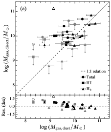
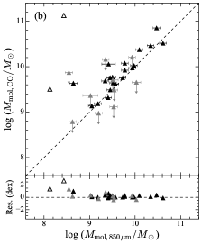
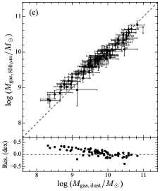
Figure 10: (a) Comparison of the directly measured gas masses with the dust-converted gas masses of PG quasars with available measurements of both CO and H I (circles), only H I (squares), or only CO (triangles). Comparing to the dust-derived total gas mass, the deviations (y$-$x) of the directly measured total (H I+$\mathrm{H}_{2}$), H I, and $\mathrm{H}_{2}$ gas masses are on average 0.47$\pm$0.08 dex, 0.43$\pm$0.10 dex, and $-0.22\pm$0.08 dex, respectively, with the $50^{+25}_{-25}$th percentile being $0.42^{+0.08}_{-0.20}$ dex, $0.39^{+0.33}_{-0.29}$ dex, and $-0.24^{+0.28}_{-0.14}$. (b) Comparison of molecular gas masses measured from CO observations with those derived from $L_{\nu_{\mathrm{850\,\mu m}}}$. The gray symbols are the objects for which only CO upper limits are available. The mean deviation (y$-$x) is 0.08$\pm$0.06; the $50^{+25}_{-25}$th percentile of the deviation is $0.05^{+0.22}_{-0.14}$ dex. The statistics above properly consider upper limits. PG 0003$+$199 and PG 1226$+$023 (empty symbols), which show large deviations from the one-to-one relation line in (a) and (b), have only marginal CO detections, and hence their CO-based molecular gas masses may have large errors; we exclude these two objects from the statistics. (c) Total gas masses estimated from the specific luminosity at $850\,\mu m$ are, on average, consistent with our total gas masses converted from dust masses: the median deviation (y$-$x) is 0.09 dex with an RMS of 0.14 dex. Since the upper limits are for both axes, we do not consider the upper limits here.

A subset of the PG quasars have published CO(1–0) (32 objects) and H I (13 objects) observations (Table 6). We calculate molecular and atomic gas masses following

$$M_{\mathrm{H2}}\,(M_{\odot})=(2.45\times 10^{3})\,\alpha_{\mathrm{CO}}\,S_{\mathrm{CO}}\Delta v\,D_{L}^{2}\,(1+z)^{-1},$$ (18)

$$M_{\mathrm{H{\sevenrm\,I}}}\,(M_{\odot})=(3.204\times 10^{5})\,D_{L}^{2}\,S_{\mathrm{H{\sevenrm\,I}}}\Delta v,$$ (19)

where $S_{\mathrm{CO}}\Delta v$ and $S_{\mathrm{H{\sevenrm\,I}}}\Delta v$ are the integrated line fluxes (Jy km s^-1), $D_{L}$ is the luminosity distance (Mpc), and $z$ is the redshift. The conversion factor $\alpha_{\mathrm{CO}}$ is still uncertain for quasar host galaxies. For consistency with the literature (Solomon et al., 1997; Evans et al., 2001), we adopt $\alpha_{\mathrm{CO}}=4.3\,M_{\odot}\,\mathrm{(K\,km\,s^{-1}\,pc^{2})^{-1}}$, the typical value of the MW disk (Bolatto et al., 2013). Helium and heavier elements are included in the gas masses.

Figure 10(a) compares the gas masses estimated from the dust mass ($M_{\mathrm{gas,dust}}$) with those derived from direct observations ($M_{\mathrm{gas,direct}}$). Since the number of objects with both CO and H I measurements is limited, we also plot separately objects with either CO or H I data only. For the objects with both CO and H I measurements, the $50^{+25}_{-25}$th percentile of the deviation between measured and dust-inferred total gas masses is $0.42^{+0.08}_{-0.20}$ dex. The excursion, however, is driven almost entirely by the H I gas. Replacing the directly measured total gas masses with H I gas masses alone, the deviation distribution becomes $0.39^{+0.33}_{-0.29}$ dex. By contrast, the deviation of CO-based $\mathrm{H}_{2}$ gas masses is $-0.24^{+0.28}_{-0.14}$ dex.

What is responsible for the discrepancy with the H I masses? We inspect the host galaxy morphology and environment of the 13 PG quasars with H I measurements using optical images from HST (Kim et al. 2008; Kim et al. 2017; Y. Zhao et al. 2018, in preparation) and SDSS. As documented in the notes of Table 6, all the eight objects with directly measured gas masses $>0.3$ dex higher than the dust-derived gas masses appear to be disturbed systems in various stages of merging. The H I line profiles of most of these objects show broad and/or asymmetric features, indicating that the target H I gas suffers confusion and/or dynamical disturbance. The remaining five objects are all likely isolated. We speculate, but cannot prove, that the H I in these merger systems may be exceptionally extended (e.g., van Gorkom et al. 1996; Geréb et al. 2016). For objects residing in dense environments (e.g., PG 0007$+$106 and PG 1119$+$120), the reported H I detections may be significantly overestimated by contamination from neighboring companions. More detailed H I observations with higher angular resolution with interferometers will be crucial to reveal the true H I gas masses of quasar host galaxies.

Scoville et al. (2014, 2016) proposed a method to estimate molecular gas masses ($M_{\mathrm{mol}}$) from the specific luminosity at rest-frame $850\,\mu m$, $L_{\mathrm{\nu,850\,\mu m}}$. The conversion factor,

$$\alpha_{\mathrm{850\,\mu m}}=\frac{L_{\mathrm{\nu,850\,\mu m}}}{M_{\mathrm{mol}}}\approx 1.1\times 10^{20}\,\mathrm{erg\,s^{-1}\,Hz^{-1}}\,M_{\odot}^{-1},$$ (20)

is empirically calibrated using low-redshift star-forming and ultraluminous IR galaxies, as well as $z\approx 2$ submillimeter galaxies. Scoville et al. (2016) used $\alpha_{\mathrm{CO}}=6.5\,M_{\odot}\,\mathrm{(K\,km\,s^{-1}\,pc^{2})^{-1}}$ to calculate the molecular gas masses of the calibration galaxies. For consistency with our convention, we multiply the original value of $\alpha_{\mathrm{850\,\mu m}}$ by a factor 1.5. We obtain $L_{\mathrm{\nu,850\,\mu m}}$ from extrapolation of the best-fit SED model. Figure 10(b) shows that the molecular gas masses estimated from $L_{\mathrm{\nu,850\,\mu m}}$ agree quite well with those derived directly from CO observations. The mean deviation is 0.08$\pm$0.06 dex with the $50^{+25}_{-25}$th percentile of the deviation $0.05^{+0.22}_{-0.14}$ dex. The deviation can easily be explained by the fact that we may have overestimated the molecular gas masses using the $\alpha_{\mathrm{CO}}$ value of the MW, which is much less massive than the quasar host galaxies. Leroy et al. (2011) find that $\alpha_{\mathrm{CO}}$ is inversely correlated with galaxy stellar mass. In addition, the incompleteness of the currently compiled sample may also bias the statistics. Note that the two most extreme outliers, PG 0003$+$199 and PG 1226$+$023, were only marginally detected. We omit these two objects in all statistics.

Hughes et al. (2017) recently provide another relation between $L_{\mathrm{\nu,850\,\mu m}}$ and the total gas mass,

$$\mathrm{log}\,M_{\mathrm{gas,850\,\mu m}}=(0.84\pm 0.02)\,\mathrm{log}\,L_{\nu,850\,\mu m}-(14.95\pm 0.54).$$ (21)

They assume $\alpha_{\mathrm{CO}}=4.6\,M_{\odot}\,\mathrm{(K\,km\,s^{-1}\,pc^{2})^{-1}}$, close enough to our choice. We use Equation (21) to estimate the total gas masses of PG quasars and compare them with the dust-derived gas masses (Figure 10(c)). The two methods are also closely consistent with each other, with median deviation 0.09$\pm$0.14 dex. The slight, systematic trend seen in Figure 10(c) stems from the sublinear slope of Equation (21).

To summarize: the gas masses of PG quasars estimated indirectly from dust masses and from the 850 $\mu$m specific luminosity are consistent with each other, as well as with the $\mathrm{H}_{2}$ masses directly measured from CO observations. Dust-inferred gas masses systematically underestimate directly measured H I gas masses, which may suffer from confusion from the low angular resolution of the existing H I observations.

Table 6: PG Quasars with Gas Measurements

Object	$S_{\mathrm{CO}}\Delta v$	$M_{\mathrm{H2}}$	$S_{\mathrm{H\,I}}\Delta v$	$W_{20}$	$M_{\mathrm{H\,I}}$	$M_{\mathrm{gas}}$	References
	(Jy km $\mathrm{s}^{-1}$)	($10^{9}M_{\odot}$)	(Jy km $\mathrm{s}^{-1}$)	(km $\mathrm{s}^{-1}$)	($10^{9}M_{\odot}$)	($10^{9}M_{\odot}$)
(1)	(2)	(3)	(4)	(5)	(6)	(7)	(8)
PG 0003$+$199	+24.7	3.2200	$<$0.35000	$\cdots$	$<$1.42	$<$4.6400	001, 10
PG 0007$+$106	0$<$3.0	$<$5.1000	0.65000	800	36.67	$<$41.7700	003, 9
PG 0050$+$124	+30.0	23.6700	1.00000	420	25.50	49.1700	005, 9
PG 0052$+$251	+02.0	10.5900	$\cdots$ 00	$\cdots$	+ $\cdots$	$\cdots$	002
PG 0157$+$001	+05.5	32.7100	$\cdots$ 00	$\cdots$	+ $\cdots$	$\cdots$	005
PG 0804$+$761	+02.0	4.3100	$\cdots$ 00	$\cdots$	+ $\cdots$	$\cdots$	004
PG 0838$+$770	+02.5	9.3700	$\cdots$ 00	$\cdots$	+ $\cdots$	$\cdots$	005
PG 0844$+$349	0$<$1.5	$<$1.3000	1.05000	488	29.60	$<$30.9000	004, 10
PG 0934$+$013	0$<$1.8	$<$0.9500	$\cdots$ 00	$\cdots$	+ $\cdots$	$\cdots$	006
PG 1011$-$040	+06.8	4.8400	$\cdots$ 00	$\cdots$	+ $\cdots$	$\cdots$	006
PG 1119$+$120	+02.7	1.3700	0.55000	310	+08.90	10.2600	005, 9
PG 1126$-$041	+07.5	5.7200	$\cdots$ 00	$\cdots$	$\cdots$	$\cdots$	006
PG 1202$+$281	0$<$2.4	$<$14.4500	$\cdots$ 00	$\cdots$	$\cdots$	$\cdots$	003
PG 1211$+$143	0$<$1.5	$<$2.3200	$<$0.05000	$\cdots$	$<$2.56	$<$4.8800	004, 9
PG 1226$+$023	+24.2	133.2800	$\cdots$ 00	$\cdots$	+ $\cdots$	$\cdots$	008
PG 1229$+$204	+02.4	2.0900	0.23000	295	+06.48	8.5700	004, 10
PG 1244$+$026	+ $\cdots$	$\cdots$	$<$0.47000	$\cdots$	$<$7.29	$\cdots$	0010
PG 1309$+$355	0$<$0.6	$<$4.5200	$\cdots$ 00	$\cdots$	+ $\cdots$	$\cdots$	002
PG 1310$-$108	0$<$2.4	$<$0.6200	$\cdots$ 00	$\cdots$	+ $\cdots$	$\cdots$	006
PG 1351$+$640	+02.7	4.3800	$\cdots$ 00	$\cdots$	+ $\cdots$	$\cdots$	005
PG 1402$+$261	+02.0	11.8900	$\cdots$ 00	$\cdots$	+ $\cdots$	$\cdots$	002
PG 1404$+$226	+02.0	4.1400	$\cdots$ 00	$\cdots$	+ $\cdots$	$\cdots$	004
PG 1411$+$442	0$<$1.8	$<$3.0600	$\cdots$ 00	$\cdots$	+ $\cdots$	$\cdots$	004
PG 1415$+$451	+02.1	5.9200	$\cdots$ 00	$\cdots$	+ $\cdots$	$\cdots$	005
PG 1426$+$015	+03.6	5.7100	0.46000	357	24.13	29.8400	004, 10
PG 1440$+$356	+06.6	8.3600	$\cdots$ 00	$\cdots$	+ $\cdots$	$\cdots$	005
PG 1444$+$407	+00.7	11.3900	$\cdots$ 00	$\cdots$	+ $\cdots$	$\cdots$	002
PG 1448$+$273	+ $\cdots$	$\cdots$	0.35000	580	10.19	$\cdots$	009
PG 1501$+$106	$<$27.3	$<$7.4100	$<$0.19000	$\cdots$	$<$1.63	$<$9.0400	001, 9
PG 1545$+$210	0$<$1.0	$<$16.1500	$\cdots$ 00	$\cdots$	+ $\cdots$	$\cdots$	002
PG 1613$+$658	+08.0	29.0500	$\cdots$ 00	$\cdots$	+ $\cdots$	$\cdots$	005
PG 1700$+$518	+03.9	71.0800	$\cdots$ 00	$\cdots$	+ $\cdots$	$\cdots$	007
PG 2130$+$099	+03.9	3.0800	0.47000	506	11.98	15.0600	005, 10
PG 2214$+$139	+01.6	1.5300	0.77000	330	23.89	25.4200	004, 9

Note. — (1) Object name. (2) $J$ band (1.235 $\mu$m) from 2MASS; (3) $H$ band (1.662 $\mu$m) from 2MASS; (4) $K_{s}$ band (2.159 $\mu$m) from 2MASS; (5) W1 band (3.353 $\mu$m) from WISE; (6) W2 band (4.603 $\mu$m) from WISE; (7) W3 band (11.561 $\mu$m) from WISE; (8) W4 band (22.088 $\mu$m) from WISE. The WISE W3 and W4 bands are corrected for a calibration discrepancy described in the text. This table is available in its entirety in a machine-readable form in the on-line journal. A portion is shown here for guidance regarding its form and content.

Note. — (1) Object name. (2) PACS 70 $\mu$m band; (3) PACS 100 $\mu$m band; (4) PACS 160 $\mu$m band; (5) SPIRE 250 $\mu$m band; (6) SPIRE 350 $\mu$m band; (7) SPIRE 500 $\mu$m band. The 5% calibration uncertainties for PACS and SPIRE photometry are not included in the uncertainties listed in the table. This table is available in its entirety in a machine-readable form in the on-line journal. A portion is shown here for guidance regarding its form and content.

Note. — This table is available in its entirety in a machine-readable form in the on-line journal. A portion is shown here for guidance regarding its form and content.

Note. — (1) The name of the model used in the paper. (2) The parameters of each model. (3) The units of the parameters. (4) Whether the parameter is discrete and requires interpolation to implement the MCMC fitting. (5) The prior range of the parameters.

Note. — (1) Object name. (2) The CO integrated line flux. (3) The molecular gas mass converted from the CO line emission, with $\alpha_{\mathrm{CO}}=4.3\,M_{\odot}\,\mathrm{(K\,km\,s^{-1}\,pc^{2})^{-1}}$. (4) The H I integrated line flux. (5) Width of the line profile measured at 20% of the peak. (6) The H I gas mass. (7) The total gas mass, $M_{\mathrm{H2}}+M_{\mathrm{H\,I}}$. $M_{\mathrm{H2}}$, $M_{\mathrm{H\,I}}$, and $M_{\mathrm{gas}}$ include helium and the heavier elements. (8) References: (1) Maiolino et al. (1997), (2) Casoli & Loinard (2001), (3) Evans et al. (2001), (4) Scoville et al. (2003), (5) Evans et al. (2006), (6) Bertram et al. (2007), (7) Evans et al. (2009), (8) Xia et al. (2012), (9) Hutchings et al. (1987), (10) Ho et al. (2008b).

Comments on the individual objects with H I observations. We search the NED and SDSS databases for the information of the nearby galaxies within (1) 7$\farcm$5 radius and (2) $\pm 2\,W_{20}$ in velocity. The host galaxy morphologies come from the HST images. PG 0003$+$199 is isolated; no comparable-size galaxies are found nearby. The host galaxy is a bulge-dominated disk galaxy (Kim et al., 2017). PG 0007$+$106 resides in a dense region. There are at least two galaxies nearby and likely contaminating the H I measurement. The H I line profile is very broad, likely due to the confusing objects. PG 0050$+$124 is an ongoing merger, although the companion galaxy is not as large. PG 0844$+$349 is merging with a disk galaxy with comparable luminosity. There are a number of faint galaxies close to the host galaxy, although their redshift information is lacking. PG 0844$+$349 is likely in a dense environment. The H I line profile is asymmetric. PG 1119$+$120 resides in a dense region. There are two clear companions. One is inside the host galaxy envelope to the northwest and the other is farther to the north. There are at least five other smaller galaxies located within a projected distance of 25$\arcsec$ of the quasar, as noted by Surace et al. (2001). The H I profile is highly asymmetric and shows a $\sim 300\,\mathrm{km\,s^{-1}}$ offset from the optical velocity. PG 1211$+$143 may have several companion galaxies $>2\arcmin$ away but we lack line-width information to be sure. The host galaxy light distribution is smooth and regular, with no sign of merger features (Kim et al., 2008). PG 1229$+$204 is relatively isolated although there is a group of three galaxies, $\sim 2\farcm 6$ to the northwest. There are also several relatively small galaxies $>5\arcmin$ away. PG 1244$+$026 resides in an isolated environment. There are no comparable-size galaxies nearby. PG 1426$+$015 is an ongoing merger during the final stages of coalescence. There are likely a number of small galaxies nearby, although redshift information is lacking. PG 1448$+$273 is an ongoing merger after coalescence. The H I profile is somewhat asymmetric. PG 1501$+$106 is also relatively isolated. There is a galaxy 4$\farcm$6 to the northeast with systematic velocity close to that of the quasar. PG 2130$+$099 displays a disturbance in the NIR (Clements, 2000). Dunlop et al. (1993) note that there are a large number of nearby companions revealed in the $K$-band image. PG 2214$+$139 displays a shell structure in deep optical images (Hong et al., 2015), indicating that the host galaxy is a recent merger remnant. There is also a galaxy of similar size 4$\farcm$9 to the southwest. Hutchings et al. (1987) note that the H I line profile is somewhat asymmetric and broad.

6 Discussion

6.1 Dust Masses from the Photometric SED Alone

The IRS spectra play a significant role in constraining the AGN dust torus component in our SED fits. However, not all AGNs have Spitzer IRS observations. Thus, it is crucial to understand how well one can measure the dust mass using only photometric data. Over the wavelength range of IRS, the WISE W3 and W4 bands alone cannot fully constrain the CLUMPY model. We reduce the flexibility of the model by fixing it to the “median” CLUMPY template, which we calculate from the entire set of best-fit torus models for the PG sample obtained from the full SED fits (Figure 11).

Using the median CLUMPY template (only varying its amplitude) along with the rest of the components (BC03, BB, and DL07), we fit the photometric SEDs (typically 13 bands) with six physical parameters for radio-quiet objects and with eight physical parameters for radio-loud objects. We fix $\gamma=0.03$ and $q_{\mathrm{PAH}}=0.47$. Since $\gamma$ is highly degenerate with the torus component, if allowed to be free, it will always try to fit the mismatch between the torus model and the data. As long as $\gamma$ is small (e.g., $<0.1$), it will not bias the fitting results. Since the photometric data do not have sufficient coverage to be particularly sensitive to PAH features, $q_{\mathrm{PAH}}$ does not affect the fitting results with any fixed value.

We compare the best-fit values of $U_{\mathrm{min}}$, $M_{d}$, and $L_{\mathrm{IR,host}}$ (the integrated IR luminosity over 8–1000 µm) obtained from the full SED and those by using the photometric SED alone (Figure 12). The three quantities measured using the two methods all follow the one-to-one relation reasonably well and do not show systematic deviations. In particular, the objects with the most robust FIR measurements (black points) have a Pearson’s correlation coefficient $r>0.9$. The relatively large scatter mainly comes from objects whose FIR SEDs barely constrain the peak of the cold dust emission. These objects, however, have correspondingly large and properly assigned uncertainties. The scatter in $U_{\mathrm{min}}$ is relatively large. The fits of the photometric SEDs seem to systematically underestimate $U_{\mathrm{min}}$, especially for low values of $U_{\mathrm{min}}$, compared to fits of the full SEDs, mainly due to the mismatch between the simple torus template and the MIR data. The dust masses themselves are not impacted. The DL07 model is insensitive to the mismatch of the MIR model as long as the FIR data constrain the cold dust emission well.

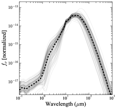
Figure 11: Best-fit CLUMPY models for the PG quasars (light gray lines) and their median value (thick dashed line), plotted on a scale with their integrated fluxes normalized to 1. Objects whose dust mass was fixed to estimate its upper limit are omitted. We use the median CLUMPY template to fit the photometric SEDs.

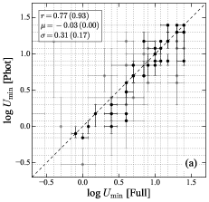
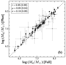
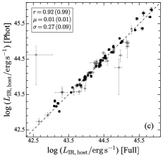
Figure 12: Comparison of fitting results for the full SED, including the IRS spectra, versus fitting only the photometric data, for the derived DL07 parameters (a) $U_{\mathrm{min}}$, (b) $M_{d}$, and (c) IR (8–1000 µm) luminosity $L_{\rm IR,host}$. Since $U_{\mathrm{min}}$ is a discrete parameter, the results are located on the dashed grids and sometimes overlap with each other; the errors are not resolvable if they are smaller than the grid size. The black points are objects with FIR data good enough to reliably constrain the DL07 model, while the gray points are the remaining objects with less robust fits. Objects with only upper limits on dust mass are omitted. The dashed line is the one-to-one relation. The upper-left corner of each panel shows the Pearson correlation coefficient ($r$) and the median ($\mu$) and standard deviation ($\sigma$) of the deviation from the linear relation. The first set of values is for the entire sample; the values for the most robust subsample (black points) are given in parentheses.

6.2 Comparison with the MBB Model

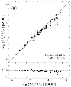
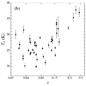
Figure 13: (a) Comparison of dust masses derived from the MBB model with those from full SED fitting with the DL07 model. We only compare the 41 radio-quiet objects with at least four Herschel bands detected. The MBB model is only applied to fit the Herschel data, excluding the 70 µm band to avoid strong contamination from warm dust. For the MBB model, we adopt the dust absorption cross-section recommended by Bianchi (2013). $M_{d}$[MBB] is offset by $-$0.04$\pm$0.11 dex relative to $M_{d}$[DL07]; the deviation is systematically larger toward higher dust masses. (b) Distribution of dust temperature versus redshift for the objects fitted with the MBB model. The apparent trend of $T_{d}$ rising for $z\approx 0.1-0.5$ may be due to the bias of warm dust (see text).

Many works use the MBB model to fit the FIR SED to estimate the dust mass and temperature (e.g., U et al. 2012; Magdis et al. 2013; Magnelli et al. 2014), assuming that the FIR emission comes from dust grains with the same size and temperature:

$$f_{\mathrm{\nu,MBB}}=\frac{(1+z)^{2}\,M_{d}\,\kappa_{\mathrm{abs}}\,B_{\nu}(T_{d})}{D_{L}^{2}},$$ (22)

where $f_{\mathrm{\nu,MBB}}$ is the rest-frame flux density, $D_{L}$ is the luminosity distance, $z$ is the redshift, and $B_{\nu}(T_{d})$ is the Planck function with dust temperature $T_{d}$. The grain absorption cross-section per unit mass $\kappa_{\mathrm{abs}}$ is usually assumed to be

$$\kappa_{\mathrm{abs}}=\kappa_{\mathrm{abs}}(\lambda_{0})\,\left(\frac{\lambda_{0}}{\lambda}\right)^{\beta},$$ (23)

where $\kappa_{\mathrm{abs}}(\lambda_{0})$ is the absorption cross-section at the given wavelength $\lambda_{0}$, calculated from MW dust models. Bianchi (2013) uses a sample of local star-forming galaxies to argue that MBB fits can provide dust masses within $\lesssim 10$% of those derived from the DL07 model, as long as $\kappa_{\mathrm{abs}}$ and $\beta$ are consistently chosen.

In order to see whether this much simpler method also works for AGN host galaxies, we use the MBB model to fit the Herschel data of PG quasars and compare the dust masses measured from the DL07 model. We limit this test to the subset of 41 objects with detections in four or more Herschel bands, with at least one detected on the Rayleigh-Jeans tail (see Appendix E). Following Bianchi (2013), we adopt $\kappa_{\mathrm{abs}}(250\,\mathrm{\mu m})=4.0~{}\mathrm{cm^{2}\,g^{-1}}$ and fix $\beta=2.08$. The median deviation between the dust masses derived from the MBB model and those from the DL07 model is $-0.04\pm 0.11$ dex (Figure 13(a)). The dust temperatures cluster around $\sim 25$ K, although $T_{d}$ seems to rise with increasing redshift for $z\approx 0.1-0.5$ (Figure 13(b)). As discussed in Appendix E, when redshift increases (especially $z>0.1$), warm dust emission increasingly affects the Herschel bands, raising $T_{d}$ and hence lowering $M_{d}$. Since more distant, more luminous objects tend to have more dust, the deviation increases systematically toward higher $M_{d}$ (Figure 13(a)). We conclude that the simple MBB method can provide robust dust masses for quasar host galaxies, as long as the SED covers the peak and Rayleigh-Jeans tail of the cold dust emission. However, one should be wary about contamination by warm dust emission and data quality. With the typical wavelength coverage and noise level of Herschel data, the MBB model can easily underestimate the dust mass by more than a factor of 2, even for moderately high-$z$ objects (e.g., $z>0.1$).

6.3 Implications for AGN Feedback

Our study shows that PG quasar host galaxies have a wide dispersion in ISM content. Most (90%) of the sample have gas mass fractions indistinguishable from those of massive star-forming galaxies. Only nine objects ($\sim$ 10% of the sample) are notably gas poor; they have $M_{\mathrm{gas}}/M_{*}\lesssim 0.01$, which is in the regime of quenched early-type galaxies (Figure 7(b)). PG 1226$+$023 (3C 273) is a flat-spectrum radio-loud quasar, while the rest are radio quiet. Six objects (PG 0026$+$129, PG 0804$+$761, PG 0923$+$201, PG 1226$+$023, PG 1416$-$129, and PG 1534$+$580) have available high-resolution HST optical images, the analysis of which indicates that the host galaxies have stellar light distributions consistent with elliptical galaxies (Kim et al. 2008; Kim et al. 2017; Y. Zhao et al. 2017, in preparation).

There are no obvious connections between gas content and AGN properties. Figure 14 shows no relationship at all between gas mass fraction and optical AGN luminosity [$\lambda L_{\lambda}$(5100 Å)] or Eddington ratio ($L_{\mathrm{bol}}/L_{\mathrm{Edd}}$). The bolometric luminosity is estimated from $L_{\mathrm{bol}}=10\,\lambda L_{\lambda}$(5100 Å) (McLure & Dunlop, 2004; Richards et al., 2006), and the Eddington luminosity is $L_{\mathrm{Edd}}=1.26\times 10^{38}(M_{\mathrm{BH}}/M_{\odot})$. In fact, the gas-deficient quasars are not the most luminous members, all having $\lambda L_{\lambda}$(5100 Å)$\lesssim 10^{45}\,\mathrm{erg\,s^{-1}}$, except PG 1226+023. The Eddington ratio of the gas-deficient quasars span a wide range and tend to lie below $L_{\mathrm{bol}}/L_{\mathrm{Edd}}\approx 0.1$. This suggests that the wide dispersion of gas fractions likely reflects the evolutionary stage of the host galaxy rather than any direct influence of AGN feedback.

Our results challenge the popular merger-driven evolutionary scenario for AGNs, wherein the cold gas content of unobscured quasars should be depleted, or at the very least diminished, toward the late stages of the merger process as a consequence of AGN feedback. If gas clumps are accelerated by the AGN above the escape velocity of the galaxy, the gas depletion time scale should be less than a few hundred Myr (e.g., Cicone et al. 2014). It is thus very surprising that we see little evidence that the quasar properties have any connection to the ISM content of the host galaxies.

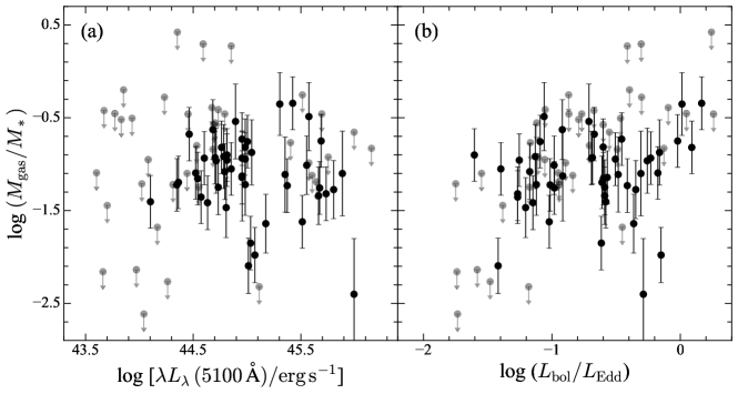
Figure 14: Dependence of the gas-to-stellar mass ratio on (a) optical (5100 Å) AGN luminosity and (b) Eddington ratio. Upper limits include sources whose dust masses are upper limits or whose host galaxy stellar masses come from the bulge masses estimated from the $M_{\mathrm{BH}}$–$M_{\mathrm{bulge}}$ relation. For clarity, the upper limits are displayed in gray.

7 Summary

The cold gas content of quasar host galaxies provides a powerful probe of the efficiency of AGN feedback. We describe our approach of inferring total gas masses from dust masses for quasars, making use of gas-to-dust ratios estimated from the stellar mass, and hence metallicity, of the host galaxies.

We construct full (1–500 µm) IR SEDs of the entire sample of 87 low-redshift ($z<0.5$) PG quasars, using photometric data from 2MASS, WISE, and Herschel, complemented by Spitzer IRS spectra. We develop a Bayesian MCMC method to simultaneously fit the photometric and spectroscopic data, using physically motivated emission components for the starlight, AGN dust torus, and large-scale galactic dust. The templates for the dust component on galactic scales are based on the dust emission models of Draine & Li (2007). The reliability of our fitting method is thoroughly investigated using mock SEDs and controlled experiments. We demonstrate that we can derive robust dust-inferred gas masses, which are unbiased with respect to gas masses obtained through other direct and indirect methods.

Our main conclusions are as follows:

1. The vast majority of quasar host galaxies are gas-rich systems, having total dust masses of $M_{d}\approx 10^{6.2}-10^{8.7}\,M_{\odot}$, with a mean value of $10^{7.6\pm 0.1}\,M_{\odot}$. These translate to total gas masses of $M_{\rm gas}\approx 10^{8.3}-10^{10.8}\,M_{\odot}$, with a mean value of $10^{9.7\pm 0.1}\,M_{\odot}$.

2. Most (90%) quasar host galaxies have similar dust and gas content to normal star-forming galaxies of similar stellar mass. Only a minority (10%) of the quasar hosts are gas-poor systems. The gas mass fraction of quasar host galaxies depends on neither the AGN luminosity nor the Eddington ratio.

3. The rich ISM content of quasars and its insensitivity to AGN properties indicate that AGN feedback is ineffective in low-redshift quasars.

4. The dust grains in quasar host galaxies appear to be exposed to a systematically stronger interstellar radiation field than normal, star-forming galaxies, suggesting that the AGN radiation field contributes to dust heating on galactic scales. We caution against the common practice of inferring star formation rates from the integrated FIR luminosity.

5. Quasar host galaxies exhibit systematically weaker PAH emission than normal galaxies. This suggests that either PAH molecules are destroyed in AGN environments or quasar hosts experience lower levels of ongoing star formation.

6. The common practice of fitting IR SEDs using modified blackbody models tends to systematically overestimate the dust temperature and underestimate the dust mass when applied to SEDs with inadequate coverage of the Rayleigh-Jeans tail of the spectrum.

Appendix A Data Systematics

In order to understand how well the WISE, Spitzer, and Herschel data match each other, we study potential systematic deviations among the three data sets. Spitzer IRS spectra cover the wavelength range of WISE W3 and W4, so we can compare the actually observed W3 and W4 flux densities with synthetic values generated from IRS spectra. To estimate the systematics of Herschel and Spitzer data, we can compare the 70 $\mu$m and 160 $\mu$m measurements of Spitzer MIPS and Herschel PACS. As the IRS spectra have been scaled to match MIPS 24 $\mu$m photometry (Shi et al., 2014), comparing MIPS and PACS at a mutual wavelength is a reasonable approach.

The WISE magnitudes are converted into monochromatic flux densities using the isophotal flux densities, $f_{\nu}\mathrm{(iso)}=f_{\nu}\mathrm{(Vega)}$ (Jarrett et al., 2011). The W3 and W4 bands are known to have a systematic, color-dependent bias: red sources (typically $f_{\nu}\propto\nu^{-2}$) are 17% fainter and 9% brighter than blue sources (typically $f_{\nu}\propto\nu^{2}$), which are used for calibration (Wright et al., 2010). Since quasars usually have $f_{\nu}\propto\nu^{-\alpha}$, with $\alpha\gtrsim 1$, we need to apply a correction to the WISE W4 flux densities (see also WISE Data Processing): $f^{\prime}_{\nu}(W4)\approx 0.90f_{\nu}(W4)$. For W3, we simply increase the $f_{\nu}(W3)$ of all objects by 17%. The corrected WISE W3 and W4 bands agree remarkably well with the Spitzer synthetic flux densities (Figure 15). Thus, we conclude that the Spitzer IRS spectra match the WISE bands very well, considering the 1.5% calibration uncertainty of WISE.

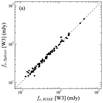
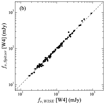
Figure 15: Comparison between flux densities from WISE and synthetic measurements of WISE bandpasses applied to Spitzer IRS spectra, for the (a) W3 and (b) W4 bands. The median deviation is 0.0$\pm$0.04 dex for W3 and 0.0$\pm$0.03 dex for W4.

We obtain the Spitzer MIPS 70 and 160 $\mu$m measurements from Shi et al. (2014) to compare with the Herschel PACS measurements (Figure 16). The Spitzer 70 $\mu$m data tend to be systematically higher than our Herschel measurements for objects $\lesssim 100$ mJy. This is likely due to confusion within the MIPS beam, which is most serious for fainter objects, because the MIPS 70 µm PSF (FWHM $\approx 18\arcsec$) is much broader than that of PACS (FWHM $\approx 6\arcsec$). The median deviation at 160 µm is $-$9%$\pm$86%. We conclude that the flux scales of Spitzer and Herschel data are well-matched to $\lesssim 10$%.

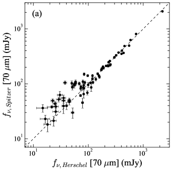
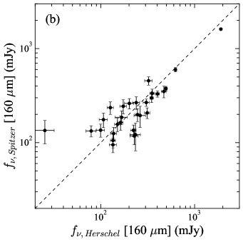
Figure 16: Comparison between flux densities from Herschel and Spitzer MIPS for the (a) 70 µm and (b) 160 µm bands. The median deviation (y$-$x) is 5%$\pm$43% for the 70 µm bands and $-$9%$\pm$86% for the 160 µm bands.

Appendix B Comparison of Herschel Data Reduction

The Herschel data for the PG sample have previously been analyzed by Petric et al. (2015). Our work is based on a completely new reduction and analysis of the same data set (Section 3), and here we present a comparison between these two independent efforts.

Petric et al. (2015) perform aperture photometry on the PACS data by summing all the pixels within a circular aperture radius of $\sim 20\arcsec$ for all three bands. They estimate uncertainties by randomly measuring the sky with the same aperture size and calculate the standard deviation of all the measurements. The large aperture size is likely to include more contaminating sources and introduce higher noise. Indeed, we find that our measurements at 70 and 100 µm are systematically lower than those of Petric et al. by 15.5% and 13.5%, respectively (Figure 17). The uncertainties of Petric et al.’s measurements are also larger than ours. The two sets of measurements at 160 µm are more consistent because the aperture sizes are comparable.

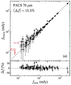
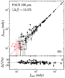
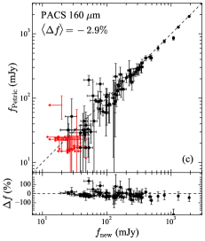
Figure 17: Comparison between our new flux densities from Herschel with those measured by Petric et al. (2015), for the PACS (a) 70 µm, (b) 100 µm, and (c) 160 µm bands. Detected sources are plotted in black, and those that are undetected by either Petric et al. or us, or both are plotted in red. The dashed line is the one-to-one relation. $\Delta f$ is the relative fractional deviation. The measurements of Petric et al. are systematically higher than ours, by $15.5\%$ at 70 µm and by $13.5\%$ at 100 µm; their uncertainties are also larger than ours. For the 160 µm band, the deviation is $-2.9\%$. This is mainly due to the aperture size effect (see the text for details).

For the reduction of the SPIRE data, Petric et al. use the Timeline Fitter to measure the sources by directly fitting the timeline data (Pearson et al., 2014). They estimate uncertainties by randomly choosing the location on the map to run the Timeline Fitter and then calculate the standard deviation. As Figure 18 shows, our measurements and those of Petric et al. are consistent within 5% for the detected sources. However, our upper limits for the undetected sources are generally higher. On the one hand, we regard a source as undetected whenever its measured flux is below $3\,\sigma$, regardless of whether the source extractor deems it to be real. On the other hand, the method used by Petric et al. to estimate the uncertainty may not be proper. Timeline Fitter is not suitable for measuring faint sources ($<30$ mJy; Pearson et al. 2014), and to estimate the uncertainty one needs to inject fake sources into the timeline (e.g., Ciesla et al. 2012) instead of fitting the timeline randomly.

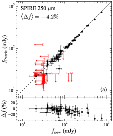
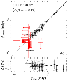
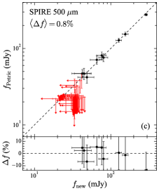
Figure 18: Comparison between our new flux densities from Herschel with those measured by Petric et al. (2015) for the SPIRE (a) 250 µm, (b) 350 µm, and (c) 500 µm bands. Detected sources are plotted in black, and those that are undetected by either Petric et al. or us, or both are plotted in red. The dashed line is the one-to-one relation. $\Delta f$ is the relative fractional deviation. The measurements of Petric et al. are consistent with ours within $\sim 5\%$ for the detected sources. However, there are also a number of notable discrepancies. Some objects are detected by our method but not by Petric et al., and vice versa.

Appendix C Fitting the SEDs with Different Dust Torus Models

We evaluate the impact of the choice of torus model on the derived parameters for the galactic dust properties. Different from the radiative transfer CLUMPY model, Xie et al. (2017) demonstrate that the IRS spectra of PG quasars can be successfully fitted by MBB models with theoretical dust absorption coefficients calculated from Mie theory (Bohren et al., 1983). We briefly summarize the XLH17 model and refer to Xie et al. (2015, 2017) for detailed discussions.

The silicate emission in the IRS spectra indicates that the dust torus is optically thin in the MIR, so that it is possible to model the torus emission without considering radiative transfer. The XLH17 model assumes that the torus consists of, on average, two chemical compositions, silicate and carbonaceous dust. We mainly use astronomical silicate (Draine & Lee, 1984) and sometimes amorphous olivine or pyroxene (Dorschner et al., 1995) for the silicate dust and graphite for the carbon dust, following the compositions suggested by XLH17. For each of the two compositions, we assume that the dust has two representative temperatures, warm and cold. The rest-frame model flux density is

$$f_{\mathrm{\nu,XLH17}}=\frac{(1+z)^{2}}{D_{L}^{2}}\sum_{i}\{B_{\nu}(T_{w,i})\,\kappa_{\mathrm{abs},i}(a_{d},\nu)\,M_{w,i}+B_{\nu}(T_{c,i})\,\kappa_{\mathrm{abs,i}}(a_{d},\nu)\,M_{c,i}\},$$ (C1)

where the summation is over two dust compositions denoted with the subscript $i$, $D_{L}$ is the luminosity distance, $\kappa_{\mathrm{abs,i}}(\nu)$ is the mass absorption coefficient for the dust with characteristic size $a_{d}$ and at frequency $\nu$, $M$ is the dust mass, and $B_{\nu}(T)$ is the Planck function with temperature $T$. The subscripts $w$ and $c$ correspond to the “warm” and “cold” dust components, respectively. The naming convention is consistent with that used in Xie et al. (2015), even though our galactic dust (DL07 component) is even colder than the “cold” torus component here. The mass ratios between carbon and silicate dust are between 0.2 and 2.0 for the warm ($r_{w,\mathrm{G/S}}$) and cold ($r_{c,\mathrm{G/S}}$) components, respectively. There are altogether nine free parameters in the XLH17 model (Table 7). The grain size $a_{d}$ is discrete, from 0.1 to 1.5 µm, while the rest of the parameters are continuous.

Table 7: The parameters and priors of the XLH17 dust torus model

Parameter	Unit	Discreteness	Prior
$a_{d}$	µm	✔	[0.1, 1.5]
$T_{w,\mathrm{sil}}$	K	✘	[250, 1500]
$M_{w,\mathrm{sil}}$	$M_{\odot}$	✘	[$10^{-5}$, $10^{8}$]
$T_{c,\mathrm{sil}}$	K	✘	[40, 200]
$M_{c,\mathrm{sil}}$	$M_{\odot}$	✘	[$10^{-5}$, $10^{8}$]
$T_{w,\mathrm{gra}}$	K	✘	[250, 1500]
$r_{w,\mathrm{G/S}}$	–	✘	[0.2, 2.0]
$T_{c,\mathrm{gra}}$	K	✘	[40, 200]
$r_{c,\mathrm{G/S}}$	–	✘	[0.2, 2.0]

For many objects, the XLH17 model performs as well, if not better, than the CLUMPY model (Figure 19(a)). However, for $\sim 1/3$ of the sample, the best-fit models show a light deficit at the short end ($\sim 7$ µm) of the IRS spectra (Figure 19(b)). This is likely due to the simplicity of the XLH17 model, which contains only four discrete temperature components, two for each composition of dust, whereas in reality the complex systems under consideration have a continuum of dust temperatures. When the temperature gaps are too large, there are light deficits in the best-fit models. This problem is not obvious if only the IRS spectrum is fitted (XLH17), but it becomes apparent when we incorporate the 2MASS and WISE bands. An extra hot component is necessary to account for the emission in NIR.

Figure 20 compares the best-fit DL07 parameters using the two torus emission models. Both yield consistent measurements of $U_{\mathrm{min}}$ and $M_{d}$, especially for objects with sufficient Herschel detections that cover well the peak and the Rayleigh-Jeans tail of the FIR SED (black points). For the rest of the objects (gray points), the scatter is considerably larger, reflecting the fact that the DL07 model is more sensitive to the torus models when the SED coverage does not provide sufficient constraints. The best-fit values of $\gamma$, as expected, show large and systematic deviations, since $\gamma$, which mainly controls the MIR emission of the DL07 model, is strongly degenerate with the torus component. The parameter $q_{\mathrm{PAH}}$ exhibits the worst performance with the XLH17 model, most likely due to its inability to properly handle the SED at wavelengths $\lesssim 7$ µm, where many PAH features lie.

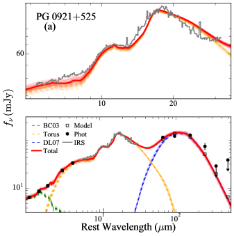
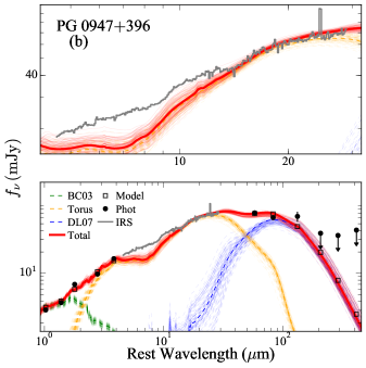
Figure 19: Examples of SED fits using the XLH17 torus model. (a) PG 0921+525 is better fit with the XLH17 model than with the CLUMPY model because the former uses an amorphous olivine model for the silicate dust. The XLH17 model is plotted as a red line, and the rest of the conventions are the same as in Figure 2. (b) By contrast, the XLH17 model does not give a good fit to the short end of the IRS spectrum for PG 0947+396. The best-fit results of the entire sample (76 objects for which the FIR data are good enough to constrain the DL07 model) can be found in the online version.

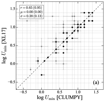
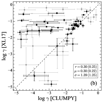
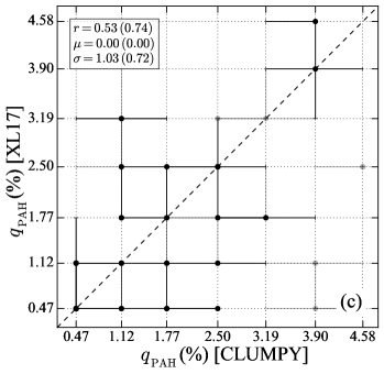
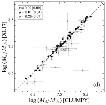
Figure 20: Comparison of the impact of the choice of torus model (XLH17 or CLUMPY) on the best-fit DL07 parameters (a) $U_{\mathrm{min}}$, (b) $\gamma$, (c) $q_{\mathrm{PAH}}$, and (d) $M_{d}$. The black points are the 44 PG quasars whose FIR data well constrain the peak and the Rayleigh-Jeans tail of the dust emission. The gray points are the 32 objects whose FIR data can still constrain the DL07 model. The dashed line is the one-to-one relation. The legend in each panel shows the Pearson correlation coefficient ($r$) and the median ($\mu$) and standard deviation ($\sigma$) of the deviation from the linear relation (y$-$x). The first set of values is for the entire sample; the values for the most robust subsample (black points) are given in parentheses. The errors of the discrete parameters ($U_{\mathrm{min}}$ and $q_{\mathrm{PAH}}$) are sometimes not resolvable if they are smaller than the grid size. The error bars for $M_{d}$ are sometimes smaller than the symbols (especially for the black points).

Appendix D Fitting and reliability

D.1 SED Fitting with emcee

In order to fit a model with up to 19 free parameters, the MCMC method is preferred to sample the posterior probability distribution to find a physically optimal solution. We use the Python package emcee (Foreman-Mackey et al., 2013), a widely used tool, to perform the MCMC sampling. This package uses the Affine Invariant MCMC Ensemble sampler to probe the parameter space with a number of “walkers.” A walker randomly proposes the next step based on the position of the other walkers. The likelihood of the new position is calculated based on the model and data. The chance for the walker to move to the new position depends on the ratio of the likelihood of the current position to that of the new position. The sequence of the positions visited by a walker forms a “chain” following the Markov process. When the chains become long enough, they can be used to construct the posterior PDF of the parameters.

Since our likelihood function is very complicated, we need to use many walkers and long enough burn-in runs in order to find the global optimum. We first use 128 walkers, initialized randomly in the parameter space allowed by the prior. Then we run the sampling three times with chain length [8000, 5000, 3000] steps as the burn-in rounds. After each burn-in round, we find the “maximum a posteriori” (MAP) and randomly initialize the walkers within a hyper-ball with a radius of 10% of the parameter prior ranges, centering at the MAP and resetting the sampler for the next round. After the first three burn-in rounds, we initialize the walkers within a hyper-ball with a radius of 1% of the prior ranges, still centered at the MAP of the previous sampling, and run another burn-in sampling with a length of 800 steps. We repeat the initialization step and run a 600 step final sampling. We drop the first 300 steps of all the walkers and use the rest of the chains ($128\times 300$ points) to define the full posterior PDF. To determine the best fit of one parameter, we marginalize the posterior PDF of all the other parameters and calculate the median. All quoted uncertainties represent the 68 percent confidence interval determined from the 16th and 84th percentiles of the marginalized posterior PDF. The strategy to run the MCMC is found effective to obtain reliable fits, although the fitting results are not sensitive to the detailed choices of the number of burn-in rounds and the length of the chains, as long as the burn-in rounds are long enough.

In the current work, we simply use uniform priors for all the parameters. Namely, for a given parameter $X$, $\mathrm{ln}\,prior=0$ for $X\in[X_{\mathrm{min}},X_{\mathrm{max}}]$, while $\mathrm{ln}\,prior=-\infty$ for $X$ out of the range. The prior ranges are chosen to be wide enough to include physically meaningful parameter ranges. It is worth mentioning that the prior ranges of the covariance model, $a$ and $\tau$, are crucial for a successful fit. In order to achieve a reasonable fitting result, the prior of $a$ should be, at most, comparable to the typical flux of the spectrum, and the prior of $\tau$ should be comparable to the length of the typical structure in the spectrum. Much wider prior ranges may lead the fit to be trapped into some unphysical solutions. Taking these considerations into account, we choose $-10<\mathrm{ln}\,a<5$ and $-5<\mathrm{ln}\,\tau<2.5$ as the fiducial priors. The lower boundaries are not important, as long as they are small enough. For some of the bright objects, we need to enlarge the prior to $-10<\mathrm{ln}\,a<10$, so that the posterior probability distribution of $\mathrm{ln}\,a$ can be a regular, Gaussian-like profile. Meanwhile, for some objects whose IRS spectra are usually not well described by the torus model, we need to constrain $a$ with a hard boundary (e.g., $\mathrm{ln}\,a<1$); otherwise, the torus model cannot match the spectrum well. For these objects (17 objects with CLUMPY model), the model-dependent uncertainty may be larger than the rest of the objects.

The ensemble sampler of emcee requires the parameters of the model to be a continuous variable. Therefore, we need to interpolate the discrete parameters that determine the precalculated templates. We use the k-Nearest Neighbor (kNN) method to overcome the discreteness of the DL07 model and the grain size of the XLH17 model. We build the K-D Tree (Bentley, 1975) with the scikit-learn package (Pedregosa et al., 2011) and find the nearest parameters of the templates for the input parameters. Since CLUMPY consists of more than $10^{6}$ templates densely sampling the relevant parameter space, we use a dedicated code (R. Nikutta 2017, private communication) to interpolate the templates with multilinear interpolation. The discreteness, especially the coarse grid, may influence the posterior probability distribution of the parameters. For example, the uncertainty of the dust mass may be underestimated because the grids of $U_{\mathrm{min}}$ are too coarse. We know that $U_{\mathrm{min}}$ and $M_{d}$ are degenerate: a smaller $U_{\mathrm{min}}$ leads to a larger $M_{d}$. Therefore, the distribution of $M_{d}$ is likely limited, since usually all of the walkers are trapped between two grid points of $U_{\mathrm{min}}$. Fully addressing this problem is beyond the scope of the current work; nevertheless, we test the reliability of our fitting code and the uncertainty estimation, as described below.

D.2 Reliability of Fitting

We generate mock SEDs based on the real data of the PG quasars. We use the best-fit parameters of each quasar to generate the SED model. We calculate the synthetic spectral and photometric data at the same rest-frame wavelengths as the real data. The uncertainties of the real SED are also used as the uncertainties of the mock SED. The mock data values are then perturbed around themselves assuming a Gaussian probability distribution with the standard deviation as the uncertainties. Sometimes, the uncertainties of some spectral points and/or Herschel photometric points are larger than one-third of the synthetic mock values. In that case, we use one-third of the mock value as the standard deviation so that the perturbation will not be too large. Some targets have upper limits in some of the Herschel bands. Their synthetic photometric data are then replaced by the real upper limits. Furthermore, we perturb the WISE, Spitzer, PACS, and SPIRE data by 3% (Jarrett et al., 2011), 5% (MIPS handbook), 5% (Balog et al., 2014), and 5% (Pearson et al., 2014), respectively, to model the calibration systematic uncertainties.

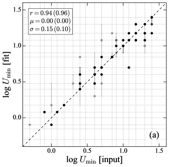
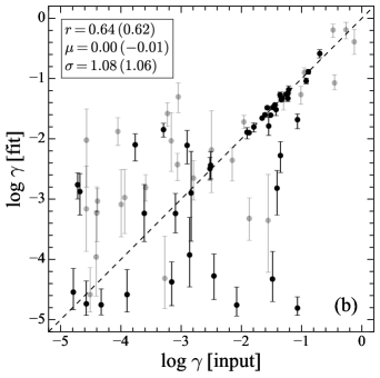
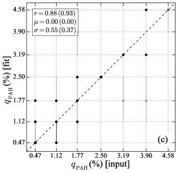
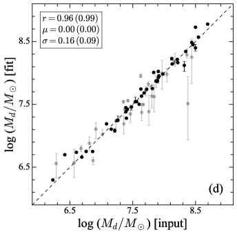
Figure 21: Fits of mock SEDs to evaluate the degree to which the input parameters of the DL07 model parameters, (a) $U_{\mathrm{min}}$, (b) $\gamma$, (c) $q_{\mathrm{PAH}}$, and (d) $M_{d}$, can be recovered. The black points are the 44 PG quasars whose FIR data well constrain the peak and the Rayleigh-Jeans tail of the dust emission. The gray points are the 29 objects whose Herschel data can still constrain the DL07 model; three objects with FIR data from the archive are not included. The dashed line is the one-to-one relation. The legend of each panel shows the Pearson correlation coefficient ($r$) and the median ($\mu$) and standard deviation ($\sigma$) of the deviation from the linear relation (y$-$x). The first set of values is for the entire sample; the values for the most robust subsample (black points) are given in parentheses. The errors of the discrete parameters ($U_{\mathrm{min}}$ and $q_{\mathrm{PAH}}$) are sometimes not resolvable if they are smaller than the grid size. The error bars for $M_{d}$ are sometimes smaller than the symbols (especially for the black points).

We fit the mock SEDs using the same method as that used for the real SEDs. The best-fit and input parameters of the DL07 model are compared in Figure 21. The input and best-fit parameters of $U_{\mathrm{min}}$, $q_{\mathrm{PAH}}$, and $M_{d}$ are tightly correlated without systematic deviation. As $U_{\mathrm{min}}$ and $q_{\mathrm{PAH}}$ are discrete parameters, we plot their grid as dotted lines. The typical scatter in $U_{\mathrm{min}}$ and $q_{\mathrm{PAH}}$ is $\lesssim 2$ grid points, especially for objects whose FIR data well constrain the peak and Rayleigh-Jeans tail of the dust emission. For $\gamma$, the correlation is reasonably good for $\gamma\gtrsim 0.01$, below which the scatter becomes large, albeit showing no systematic deviation. The reasons are as follows: (1) $\gamma$ mainly controls the MIR emission of the DL07 model, while the MIR emission of the quasar is dominated by the AGN torus; (2) $\gamma$ is usually small, rendering it more sensitive to mismatch between the torus model and the spectra; (3) systematic uncertainties in the IRS spectra with respect to the FIR data may lead to a large error on $\gamma$, especially when it is small. In view of these complications, we should exercise caution in interpreting the results of $\gamma$.

As just mentioned, the uncertainties of the fitting results may not reflect their true errors for parameters that are discrete. For example, in the case of $U_{\mathrm{min}}$, even some of the robust fits with small error bars (black points in Figure 21) deviate from the one-to-one line by two grid points. The same holds for $M_{d}$. The situation is not as serious for the less robust fits (gray points). Note that the primary goal of this study is to derive gas masses, whose final uncertainty is likely dominated by the uncertainty in $\delta_{\mathrm{GDR}}$, especially the unknown systematic uncertainty due to the H I gas distribution (Section 5.3.2). As the exact dust mass uncertainty will not affect our main conclusions, we will directly quote its value provided by our MCMC code. Future refinement of the parameter grids of the DL07 templates would be valuable to obtain more accurate dust masses.

Figure 22 demonstrates that our fitting method can robustly decompose the dust torus emission to yield accurate measurements of the integrated IR (8–1000 µm) luminosity of the galactic dust emission, as well as the specific luminosity at 850 µm. Besides the DL07 parameters, we do not discuss other model components, which are not the primary focus of this study. We simply note, in passing, that the input parameters of the CLUMPY torus model—apart from the optical depth $\tau_{V}$—are usually not well-reproduced by the fits, most likely because of the degeneracy with the ad hoc hot dust (BB) component. A more comprehensive dust torus model (e.g., García-González et al. 2017; Hönig & Kishimoto 2017) is needed if we wish to truly study the properties of the AGN torus using the SED fitting method. From the posterior PDF of the parameters, we do not observe a clear degeneracy between the parameters of DL07 and the other components (e.g., CLUMPY). This is likely because (1) the IRS spectra effectively constrain the CLUMPY and DL07 models, so they cannot vary as freely as the fittings with photometric data only, (2) the discreteness of $U_{\mathrm{min}}$ dominates the parameter uncertainties of DL07. As shown in Table 1, the uncertainties of $U_{\mathrm{min}}$ are often unresolved. Unless the parameter space of the DL07 templates is refined, it is hard to analyze the degeneracies between the CLUMPY and DL07 parameters. Therefore, with the current models, the degeneracy of the torus and DL07 parameters is dominated by the systematics from different torus models adopted in the fitting. As discussed in Appendix C, this does not significantly affect $U_{\mathrm{min}}$ and $M_{d}$, especially when the FIR data are good enough to constrain the peak of the SED. More comparisons of the SED fits with different torus models will be presented in a forthcoming work (Zhuang et al., 2017).

In summary: our SED fitting method can reliably measure $U_{\mathrm{min}}$, $q_{\mathrm{PAH}}$, and $M_{d}$ for nearly the entire sample of PG quasars, except for those with insufficient FIR data to constrain the DL07 model well.

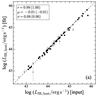
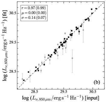
Figure 22: Fits of mock SEDs to evaluate the degree to which the total IR (8–1000 µm) luminosity ($L_{\rm IR,host}$) and specific luminosity at 850 µm ($L_{\mathrm{\nu,850\,\mu m}}$) can be recovered using the DL07 model. Symbols and conventions same as in Figure 21.

Appendix E Systematics of Fitting the SED with MBB Model

We study the possible factors that might bias the dust mass $M_{d}$ and dust temperature $T_{d}$ when the SED is fitted with an MBB model, a common practice in the literature. We generate mock SEDs using the DL07 model with different parameters and redshift. The SED contains the Herschel bands between 100 and 500 µm. We also consider different levels of data quality, including the impact of upper limits. We first summarize our conclusions:

1. The shortest-wavelength (100 $\mu$m) band is easily contaminated by emission from warm dust, such that $T_{d}$ is biased toward higher values and $M_{d}$ is underestimated. This effect becomes serious when $\gamma$ is high, $U_{\mathrm{min}}$ is low, or the redshift is high. The parameter $q_{\mathrm{PAH}}$ only marginally affects the fitting. This bias in principle can be mitigated by dropping the 100 µm band from the fit, but in practice this benefit is offset by the larger uncertainties or upper limits often encountered in the 160–500 µm bands.

2. The SED can hardly constrain $M_{d}$ and $T_{d}$ when there are two or more upper limits at the longest bands. As the data mainly constrain the Rayleigh-Jeans tail, the fits tend to overestimate $T_{d}$ and underestimate $M_{d}$.

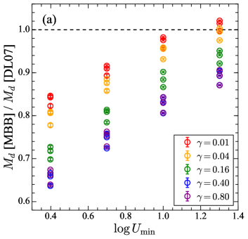
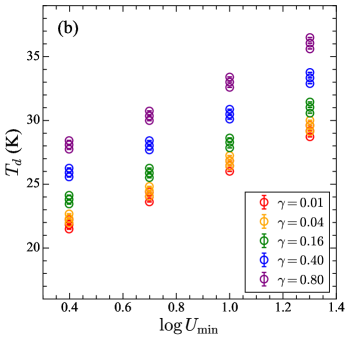
Figure 23: Variation with $U_{\mathrm{min}}$ and $\gamma$ of (a) the dust mass derived from the best-fit MBB model relative to that derived from the DL07 model and (b) the dust temperature of the best-fit MBB model. Below the dashed line, the MBB model underestimates the dust mass. Each combination ($U_{\mathrm{min}}$, $\gamma$) contains three values of $q_{\mathrm{PAH}}$.

We generate mock SEDs using the DL07 model with different values of $U_{\mathrm{min}}$ (2.5, 5, 10, 20), $\gamma$ (0.01, 0.04, 0.16, 0.4, 0.8), and $q_{\mathrm{PAH}}$ (0.47, 2.5, 4.58) and fit them with the MBB model (Figure 23). Fixing $\gamma$, the ratio of dust masses derived from the MBB fit to the fiducial value from the DL07 model, $M_{d}$[MBB]/$M_{d}$[DL07], decreases as $U_{\mathrm{min}}$ decreases (Figure 23(a)). This reflects the fact that when $U_{\mathrm{min}}$ decreases, the FIR SED tends to peak at longer wavelengths ($>100\,\mu m$), such that more warm dust emission on the shorter-wavelength side of the peak enters the 100 µm band. Note that although $T_{d}$ and $U_{\mathrm{min}}$ are positively correlated (Figure 23(b)), as they should be, when $U_{\mathrm{min}}$ is low, the $T_{d}$ from the MBB fitting is biased to temperatures higher than it should be, due to the warm dust contamination. On the other hand, at fixed $U_{\mathrm{min}}$, $M_{d}$ is increasingly underestimated when $\gamma$ increases. Comparing the two panels of Figure 23, it is clear that higher values of $\gamma$ induce more contamination by warm dust in the 100 $\mu$m band, which, in turn, leads to a higher $T_{d}$ and hence lower $M_{d}$. The parameter $q_{\mathrm{PAH}}$ has only a minor effect on $M_{d}$ and $T_{d}$.

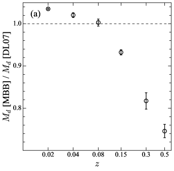
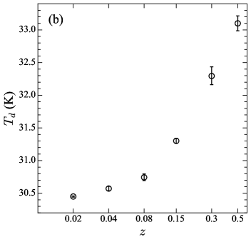
Figure 24: Variation with redshift $z$ of (a) the dust mass derived from the best-fit MBB model relative to that derived from the DL07 model and (b) dust temperature of the best-fit MBB model. Below the dashed line, the MBB model underestimates the dust mass.

In order to quantify the effect of redshift, we generate mock SEDs for different values of $z$ (0.02, 0.04, 0.08, 0.15, 0.3, 0.5) with a fixed set of fiducial DL07 model parameters ($U_{\mathrm{min}}=25$, $q_{\mathrm{PAH}}=0.47$, $\gamma=0$, $M_{d}=10^{8.1}\,M_{\odot}$). Then, we fit the MBB model to the 100–500 µm SED. The best-fit $M_{d}$ decreases and $T_{d}$ increases as $z$ increases (Figure 24), as a consequence of increased contamination from warm dust emission when the peak of the SED shifts redward.

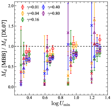
Figure 25: Dust mass derived from the best-fit MBB model relative to that derived from the DL07 model as a function of $U_{\mathrm{min}}$ and $\gamma$. The different symbols denote SEDs with different numbers of upper limits in their spectral coverage. Starting from the longest wavelength, circle = 0, square = 1, triangle = 2, and cross = 3 upper limits, respectively. For clarity, points with the same value of $U_{\mathrm{min}}$ are offset slightly in the horizontal direction.

Finally, we generate mock SEDs with different numbers of upper limits (0, 1, 2, 3) to study the effect of non-detections on SED fits with the MBB model (Figure 25). Comparing the error bars and scatter of the different symbols, it is clear that the uncertainty of the fits becomes larger when there are more upper limits in the SED. In particular, the scatter is unacceptably large when there are as many as three upper limits. In general, as the number of upper limits increases toward longer wavelengths, the Rayleigh-Jeans tail becomes more and more poorly constrained, $T_{d}$ is more easily overestimated, and $M_{d}$ becomes systematically more underestimated.

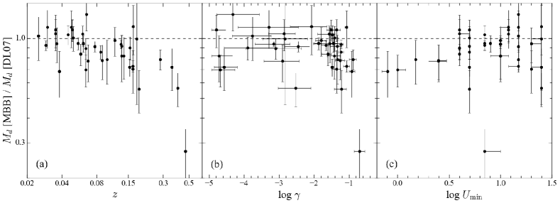
Figure 26: Variation of the dust mass derived from the MBB model relative to that derived from the DL07 model as a function of (a) $z$, (b) $\gamma$, and (c) $U_{\mathrm{min}}$. The mass ratio is apparently decreasing toward higher $z$ and higher $\gamma$, for $\log\gamma>-2$. There is no obvious trend with $U_{\mathrm{min}}$.

For the PG quasars with $\geq 4$ detections in the Herschel bands, the dependence of $M_{d}$[MBB]/$M_{d}$[DL07] on DL07 parameters is shown in Figure 26. It seems that $z$ and $\gamma$ are the main culprits for the underestimation of $M_{d}$[MBB]. Since $\gamma$ is easily biased in the fitting, we are unsure whether or not the trend with $\gamma$ is real. The trend with $z$, however, is robust. The $U_{\mathrm{min}}$ parameter does not significantly influence $M_{d}$[MBB]/$M_{d}$[DL07], except that it becomes systematically lower than 1 when $\mathrm{log}\,U_{\mathrm{min}}<0.5$.

References

- Ambikasaran et al. (2014) Ambikasaran, S., Foreman-Mackey, D., Greengard, L., Hogg, D. W., & O’Neil, M. 2014, arXiv:1403.6015
- Astropy Collaboration et al. (2013) Astropy Collaboration, Robitaille, T. P., Tollerud, E. J., et al. 2013, A&A, 558, A33
- Balog et al. (2014) Balog, Z., Müller, T., Nielbock, M., et al. 2014, Experimental Astronomy, 37, 129
- Bentley (1975) Bentley, J. L. 1975, Commun. ACM, 18, 509. http://doi.acm.org/10.1145/361002.361007
- Berta et al. (2016) Berta, S., Lutz, D., Genzel, R., Förster-Schreiber, N. M., & Tacconi, L. J. 2016, A&A, 587, A73
- Berta et al. (2013) Berta, S., Lutz, D., Santini, P., et al. 2013, A&A, 551, A100
- Bertram et al. (2007) Bertram, T., Eckart, A., Fischer, S., et al. 2007, A&A, 470, 571
- Bessell & Murphy (2012) Bessell, M., & Murphy, S. 2012, PASP, 124, 140
- Bianchi (2013) Bianchi, S. 2013, A&A, 552, A89
- Bianchi et al. (2009) Bianchi, S., Guainazzi, M., Matt, G., Fonseca Bonilla, N., & Ponti, G. 2009, A&A, 495, 421
- Bigiel et al. (2008) Bigiel, F., Leroy, A., Walter, F., et al. 2008, AJ, 136, 2846
- Bohren et al. (1983) Bohren, C. F., Huffman, D. R., & Kam, Z. 1983, Nature, 306, 625
- Bolatto et al. (2013) Bolatto, A. D., Wolfire, M., & Leroy, A. K. 2013, ARA&A, 51, 207
- Boroson & Green (1992) Boroson, T. A., & Green, R. F. 1992, ApJS, 80, 109
- Boselli et al. (2014a) Boselli, A., Cortese, L., & Boquien, M. 2014a, A&A, 564, A65
- Boselli et al. (2014b) Boselli, A., Cortese, L., Boquien, M., et al. 2014b, A&A, 564, A66
- Boselli et al. (2010) Boselli, A., Eales, S., Cortese, L., et al. 2010, PASP, 122, 261
- Boselli et al. (2002) Boselli, A., Lequeux, J., & Gavazzi, G. 2002, A&A, 384, 33
- Bruzual & Charlot (2003) Bruzual, G., & Charlot, S. 2003, MNRAS, 344, 1000
- Calistro Rivera et al. (2016) Calistro Rivera, G., Lusso, E., Hennawi, J. F., & Hogg, D. W. 2016, ApJ, 833, 98
- Carniani et al. (2016) Carniani, S., Marconi, A., Maiolino, R., et al. 2016, A&A, 591, A28
- Casoli & Loinard (2001) Casoli, F., & Loinard, L. 2001, in Astronomical Society of the Pacific Conference Series, Vol. 235, Science with the Atacama Large Millimeter Array, ed. A. Wootten, 305
- Chabrier (2003) Chabrier, G. 2003, PASP, 115, 763
- Chini et al. (1989) Chini, R., Biermann, P. L., Kreysa, E., & Gemuend, H.-P. 1989, A&A, 221, L3
- Cicone et al. (2014) Cicone, C., Maiolino, R., Sturm, E., et al. 2014, A&A, 562, A21
- Ciesla et al. (2014) Ciesla, L., Boquien, M., Boselli, A., et al. 2014, A&A, 565, A128
- Ciesla et al. (2012) Ciesla, L., Boselli, A., Smith, M. W. L., et al. 2012, A&A, 543, A161
- Ciesla et al. (2015) Ciesla, L., Charmandaris, V., Georgakakis, A., et al. 2015, A&A, 576, A10
- Clements (2000) Clements, D. L. 2000, MNRAS, 311, 833
- Cohen et al. (2007) Cohen, A. S., Lane, W. M., Cotton, W. D., et al. 2007, AJ, 134, 1245
- Cohen et al. (2003) Cohen, M., Wheaton, W. A., & Megeath, S. T. 2003, AJ, 126, 1090
- Condon et al. (1998) Condon, J. J., Cotton, W. D., Greisen, E. W., et al. 1998, AJ, 115, 1693
- Cortese et al. (2016) Cortese, L., Bekki, K., Boselli, A., et al. 2016, MNRAS, 459, 3574
- Cortese et al. (2012) Cortese, L., Ciesla, L., Boselli, A., et al. 2012, A&A, 540, A52
- Cortese et al. (2010) Cortese, L., Davies, J. I., Pohlen, M., et al. 2010, A&A, 518, L49
- Cresci et al. (2015) Cresci, G., Mainieri, V., Brusa, M., et al. 2015, ApJ, 799, 82
- Cutri et al. (2012) Cutri, R. M., Wright, E. L., Conrow, T., et al. 2012, Explanatory Supplement to the WISE All-Sky Data Release Products, Tech. rep. 1
- Czekala et al. (2015) Czekala, I., Andrews, S. M., Mandel, K. S., Hogg, D. W., & Green, G. M. 2015, ApJ, 812, 128
- Dale et al. (2012) Dale, D. A., Aniano, G., Engelbracht, C. W., et al. 2012, ApJ, 745, 95
- Dale et al. (2017) Dale, D. A., Cook, D. O., Roussel, H., et al. 2017, ApJ, 837, 90
- Deo et al. (2011) Deo, R. P., Richards, G. T., Nikutta, R., et al. 2011, ApJ, 729, 108
- Dorschner et al. (1995) Dorschner, J., Begemann, B., Henning, T., Jaeger, C., & Mutschke, H. 1995, A&A, 300, 503
- Douglas et al. (1996) Douglas, J. N., Bash, F. N., Bozyan, F. A., Torrence, G. W., & Wolfe, C. 1996, AJ, 111, 1945
- Downes & Solomon (1998) Downes, D., & Solomon, P. M. 1998, ApJ, 507, 615
- Draine et al. (2007) Draine, B. T., Dale, D. A., Bendo, G., et al. 2007, ApJ, 663, 866
- Draine & Lee (1984) Draine, B. T., & Lee, H. M. 1984, ApJ, 285, 89
- Draine & Li (2007) Draine, B. T., & Li, A. 2007, ApJ, 657, 810
- Dubois et al. (2016) Dubois, Y., Peirani, S., Pichon, C., et al. 2016, MNRAS, 463, 3948
- Dunlop et al. (1993) Dunlop, J. S., Taylor, G. L., Hughes, D. H., & Robson, E. I. 1993, MNRAS, 264, 455
- Eales et al. (2012) Eales, S., Smith, M. W. L., Auld, R., et al. 2012, ApJ, 761, 168
- Evans et al. (2001) Evans, A. S., Frayer, D. T., Surace, J. A., & Sanders, D. B. 2001, AJ, 121, 1893
- Evans et al. (2009) Evans, A. S., Hines, D. C., Barthel, P., et al. 2009, AJ, 138, 262
- Evans et al. (2006) Evans, A. S., Solomon, P. M., Tacconi, L. J., Vavilkin, T., & Downes, D. 2006, AJ, 132, 2398
- Fabian (2012) Fabian, A. C. 2012, ARA&A, 50, 455
- Feigelson & Nelson (1985) Feigelson, E. D., & Nelson, P. I. 1985, ApJ, 293, 192
- Ferrarese & Merritt (2000) Ferrarese, L., & Merritt, D. 2000, ApJ, 539, L9
- Foreman-Mackey et al. (2013) Foreman-Mackey, D., Hogg, D. W., Lang, D., & Goodman, J. 2013, PASP, 125, 306
- García-González et al. (2017) García-González, J., Alonso-Herrero, A., Hönig, S. F., et al. 2017, MNRAS, 470, 2578
- Gebhardt et al. (2000) Gebhardt, K., Bender, R., Bower, G., et al. 2000, ApJ, 539, L13
- Geréb et al. (2016) Geréb, K., Catinella, B., Cortese, L., et al. 2016, MNRAS, 462, 382
- Goldschmidt et al. (1992) Goldschmidt, P., Miller, L., La Franca, F., & Cristiani, S. 1992, MNRAS, 256, 65P
- González-Alfonso et al. (2017) González-Alfonso, E., Fischer, J., Spoon, H. W. W., et al. 2017, ApJ, 836, 11
- Gower et al. (1967) Gower, J. F. R., Scott, P. F., & Wills, D. 1967, MmRAS, 71, 49
- Greene et al. (2011) Greene, J. E., Zakamska, N. L., Ho, L. C., & Barth, A. J. 2011, ApJ, 732, 9
- Gregory (2005) Gregory, P. C. 2005, Bayesian Logical Data Analysis for the Physical Sciences: A Comparative Approach with ‘Mathematica’ Support (Cambridge: Cambridge Univ. Press)
- Gregory & Condon (1991) Gregory, P. C., & Condon, J. J. 1991, ApJS, 75, 1011
- Griffin et al. (2010) Griffin, M. J., Abergel, A., Abreu, A., et al. 2010, A&A, 518, L3
- Han & Han (2014) Han, Y., & Han, Z. 2014, ApJS, 215, 2
- Haynes & Giovanelli (1984) Haynes, M. P., & Giovanelli, R. 1984, AJ, 89, 758
- Heckman & Best (2014) Heckman, T. M., & Best, P. N. 2014, ARA&A, 52, 589
- Henry & Worthey (1999) Henry, R. B. C., & Worthey, G. 1999, PASP, 111, 919
- Herrero-Illana et al. (2017) Herrero-Illana, R., Pérez-Torres, M. Á., Randriamanakoto, Z., et al. 2017, MNRAS, 471, 1634
- Ho et al. (2008a) Ho, L. C., Darling, J., & Greene, J. E. 2008a, ApJ, 681, 128
- Ho et al. (2008b) Ho, L. C., Darling, J., & Greene, J. E. 2008b, ApJS, 177, 103
- Ho & Kim (2009) Ho, L. C., & Kim, M. 2009, ApJS, 184, 398
- Ho & Kim (2015) Ho, L. C., & Kim, M. 2015, ApJ, 809, 123
- Hong et al. (2015) Hong, J., Im, M., Kim, M., & Ho, L. C. 2015, ApJ, 804, 34
- Hönig & Kishimoto (2010) Hönig, S. F., & Kishimoto, M. 2010, A&A, 523, A27
- Hönig & Kishimoto (2017) Hönig, S. F., & Kishimoto, M. 2017, ApJ, 838, L20
- Hopkins et al. (2006) Hopkins, P. F., Hernquist, L., Cox, T. J., et al. 2006, ApJS, 163, 1
- Hopkins et al. (2008) Hopkins, P. F., Hernquist, L., Cox, T. J., & Kereš, D. 2008, ApJS, 175, 356
- Hughes et al. (2017) Hughes, T. M., Ibar, E., Villanueva, V., et al. 2017, MNRAS, 468, L103
- Husemann et al. (2017) Husemann, B., Davis, T. A., Jahnke, K., et al. 2017, MNRAS, 470, 1570
- Husemann et al. (2014) Husemann, B., Jahnke, K., Sánchez, S. F., et al. 2014, MNRAS, 443, 755
- Hutchings et al. (1987) Hutchings, J. B., Gower, A. C., & Price, R. 1987, AJ, 93, 6
- Into & Portinari (2013) Into, T., & Portinari, L. 2013, MNRAS, 430, 2715
- Isobe et al. (1986) Isobe, T., Feigelson, E. D., & Nelson, P. I. 1986, ApJ, 306, 490
- Jarrett et al. (2003) Jarrett, T. H., Chester, T., Cutri, R., Schneider, S. E., & Huchra, J. P. 2003, AJ, 125, 525
- Jarrett et al. (2011) Jarrett, T. H., Cohen, M., Masci, F., et al. 2011, ApJ, 735, 112
- Kauffmann et al. (2003) Kauffmann, G., Heckman, T. M., Tremonti, C., et al. 2003, MNRAS, 346, 1055
- Kellermann et al. (1994) Kellermann, K. I., Sramek, R. A., Schmidt, M., Green, R. F., & Shaffer, D. B. 1994, AJ, 108, 1163
- Kellermann et al. (1989) Kellermann, K. I., Sramek, R., Schmidt, M., Shaffer, D. B., & Green, R. 1989, AJ, 98, 1195
- Kennicutt et al. (2011) Kennicutt, R. C., Calzetti, D., Aniano, G., et al. 2011, PASP, 123, 1347
- Kewley & Ellison (2008) Kewley, L. J., & Ellison, S. L. 2008, ApJ, 681, 1183
- Kim et al. (2017) Kim, M., Ho, L. C., Peng, C. Y., Barth, A. J., & Im, M. 2017, ApJS, 232, 21
- Kim et al. (2008) Kim, M., Ho, L. C., Peng, C. Y., et al. 2008, ApJ, 687, 767
- Kirkpatrick et al. (2015) Kirkpatrick, A., Pope, A., Sajina, A., et al. 2015, ApJ, 814, 9
- Kormendy & Ho (2013) Kormendy, J., & Ho, L. C. 2013, ARA&A, 51, 511
- Kraemer et al. (2011) Kraemer, S. B., Schmitt, H. R., Crenshaw, D. M., et al. 2011, ApJ, 727, 130
- Kroupa (1998) Kroupa, P. 1998, in ASP Conf. Ser. 134, Brown Dwarfs and Extrasolar Planets, ed. R. Rebolo, E. L. Martin, & M. R. Zapatero Osorio (San Francisco, CA: ASP), 483
- Kroupa (2001) Kroupa, P. 2001, MNRAS, 322, 231
- Kroupa et al. (1993) Kroupa, P., Tout, C. A., & Gilmore, G. 1993, MNRAS, 262, 545
- Large et al. (1981) Large, M. I., Mills, B. Y., Little, A. G., Crawford, D. F., & Sutton, J. M. 1981, MNRAS, 194, 693
- Larson et al. (2016) Larson, K. L., Sanders, D. B., Barnes, J. E., et al. 2016, ApJ, 825, 128
- Lavalley et al. (1992) Lavalley, M., Isobe, T., & Feigelson, E. 1992, in ASP Conf. Ser. 25, Astronomical Data Analysis Software and Systems I, ed. D. M. Worrall, C. Biemesderfer, & J. Barnes (San Francisco, CA: ASP), 245
- Lebouteiller et al. (2015) Lebouteiller, V., Barry, D. J., Goes, C., et al. 2015, ApJS, 218, 21
- Leipski et al. (2014) Leipski, C., Meisenheimer, K., Walter, F., et al. 2014, ApJ, 785, 154
- Leroy et al. (2011) Leroy, A. K., Bolatto, A., Gordon, K., et al. 2011, ApJ, 737, 12
- Lyu et al. (2016) Lyu, J., Rieke, G. H., & Alberts, S. 2016, ApJ, 816, 85
- Madau & Dickinson (2014) Madau, P., & Dickinson, M. 2014, ARA&A, 52, 415
- Magdis et al. (2012) Magdis, G. E., Daddi, E., Béthermin, M., et al. 2012, ApJ, 760, 6
- Magdis et al. (2017) Magdis, G. E., Rigopoulou, D., Daddi, E., et al. 2017, A&A, 603, A93
- Magdis et al. (2013) Magdis, G. E., Rigopoulou, D., Helou, G., et al. 2013, A&A, 558, A136
- Magnelli et al. (2014) Magnelli, B., Lutz, D., Saintonge, A., et al. 2014, A&A, 561, A86
- Magorrian et al. (1998) Magorrian, J., Tremaine, S., Richstone, D., et al. 1998, AJ, 115, 2285
- Maiolino et al. (1997) Maiolino, R., Ruiz, M., Rieke, G. H., & Papadopoulos, P. 1997, ApJ, 485, 552
- Maiolino et al. (2017) Maiolino, R., Russell, H. R., Fabian, A. C., et al. 2017, Nature, 544, 202
- Mancone & Gonzalez (2012) Mancone, C. L., & Gonzalez, A. H. 2012, PASP, 124, 606
- Marshall et al. (2007) Marshall, J. A., Herter, T. L., Armus, L., et al. 2007, ApJ, 670, 129
- Mattsson & Andersen (2012) Mattsson, L., & Andersen, A. C. 2012, MNRAS, 423, 38
- McLure & Dunlop (2004) McLure, R. J., & Dunlop, J. S. 2004, MNRAS, 352, 1390
- Mentuch Cooper et al. (2012) Mentuch Cooper, E., Wilson, C. D., Foyle, K., et al. 2012, ApJ, 755, 165
- Mor & Netzer (2012) Mor, R., & Netzer, H. 2012, MNRAS, 420, 526
- Mor et al. (2009) Mor, R., Netzer, H., & Elitzur, M. 2009, ApJ, 705, 298
- Muñoz-Mateos et al. (2009) Muñoz-Mateos, J. C., Gil de Paz, A., Boissier, S., et al. 2009, ApJ, 701, 1965
- Mullaney et al. (2011) Mullaney, J. R., Alexander, D. M., Goulding, A. D., & Hickox, R. C. 2011, MNRAS, 414, 1082
- Nenkova et al. (2008a) Nenkova, M., Sirocky, M. M., Ivezić, Ž., & Elitzur, M. 2008a, ApJ, 685, 147
- Nenkova et al. (2008b) Nenkova, M., Sirocky, M. M., Nikutta, R., Ivezić, Ž., & Elitzur, M. 2008b, ApJ, 685, 160
- Nesvadba et al. (2017) Nesvadba, N. P. H., De Breuck, C., Lehnert, M. D., Best, P. N., & Collet, C. 2017, A&A, 599, A123
- Nguyen et al. (2010) Nguyen, H. T., Schulz, B., Levenson, L., et al. 2010, A&A, 518, L5
- Noll et al. (2009) Noll, S., Burgarella, D., Giovannoli, E., et al. 2009, A&A, 507, 1793
- Ott (2010) Ott, S. 2010, in ASP Conf. Ser. 434, Astronomical Data Analysis Software and Systems XIX, ed. Y. Mizumoto, K.-I. Morita, & M. Ohishi (San Francisco, CA: ASP), 139
- Pappalardo et al. (2012) Pappalardo, C., Bianchi, S., Corbelli, E., et al. 2012, A&A, 545, A75
- Pearson et al. (2014) Pearson, C., Lim, T., North, C., et al. 2014, Experimental Astronomy, 37, 175
- Pedregosa et al. (2011) Pedregosa, F., Varoquaux, G., Gramfort, A., et al. 2011, Journal of Machine Learning Research, 12, 2825
- Pe’er (2014) Pe’er, A. 2014, Space Sci. Rev., 183, 371
- Peng et al. (2002) Peng, C. Y., Ho, L. C., Impey, C. D., & Rix, H.-W. 2002, AJ, 124, 266
- Peng et al. (2010) Peng, C. Y., Ho, L. C., Impey, C. D., & Rix, H.-W. 2010, AJ, 139, 2097
- Perna et al. (2015) Perna, M., Brusa, M., Salvato, M., et al. 2015, A&A, 583, A72
- Petric et al. (2015) Petric, A. O., Ho, L. C., Flagey, N. J. M., & Scoville, N. Z. 2015, ApJS, 219, 22
- Pettini & Pagel (2004) Pettini, M., & Pagel, B. E. J. 2004, MNRAS, 348, L59
- Pilbratt et al. (2010) Pilbratt, G. L., Riedinger, J. R., Passvogel, T., et al. 2010, A&A, 518, L1
- Planck Collaboration et al. (2016) Planck Collaboration, Ade, P. A. R., Aghanim, N., et al. 2016, A&A, 594, A13
- Podigachoski et al. (2015) Podigachoski, P., Barthel, P. D., Haas, M., et al. 2015, A&A, 575, A80
- Poglitsch et al. (2010) Poglitsch, A., Waelkens, C., Geis, N., et al. 2010, A&A, 518, L2
- Rasmussen & Williams (2016) Rasmussen, C. E., & Williams, C. K. I. 2006, Gaussian Processes for Machine Learning (Cambridge, MA: MIT)
- Reeves & Turner (2000) Reeves, J. N., & Turner, M. J. L. 2000, MNRAS, 316, 234
- Rémy-Ruyer et al. (2014) Rémy-Ruyer, A., Madden, S. C., Galliano, F., et al. 2014, A&A, 563, A31
- Richards et al. (2006) Richards, G. T., Lacy, M., Storrie-Lombardi, L. J., et al. 2006, ApJS, 166, 470
- Rowlands et al. (2015) Rowlands, K., Wild, V., Nesvadba, N., et al. 2015, MNRAS, 448, 258
- Saintonge et al. (2016) Saintonge, A., Catinella, B., Cortese, L., et al. 2016, MNRAS, 462, 1749
- Saintonge et al. (2011) Saintonge, A., Kauffmann, G., Kramer, C., et al. 2011, MNRAS, 415, 32
- Saintonge et al. (2012) Saintonge, A., Tacconi, L. J., Fabello, S., et al. 2012, ApJ, 758, 73
- Sales et al. (2010) Sales, D. A., Pastoriza, M. G., & Riffel, R. 2010, ApJ, 725, 605
- Sales et al. (2015) Sales, D. A., Robinson, A., Axon, D. J., et al. 2015, ApJ, 799, 25
- Salpeter (1955) Salpeter, E. E. 1955, ApJ, 121, 161
- Sanders et al. (1988) Sanders, D. B., Soifer, B. T., Elias, J. H., et al. 1988, ApJ, 325, 74
- Santini et al. (2014) Santini, P., Maiolino, R., Magnelli, B., et al. 2014, A&A, 562, A30
- Savage & Oliver (2007) Savage, R. S., & Oliver, S. 2007, ApJ, 661, 1339
- Schmidt & Green (1983) Schmidt, M., & Green, R. F. 1983, ApJ, 269, 352
- Schweitzer et al. (2008) Schweitzer, M., Groves, B., Netzer, H., et al. 2008, ApJ, 679, 101
- Scoville et al. (2014) Scoville, N., Aussel, H., Sheth, K., et al. 2014, ApJ, 783, 84
- Scoville et al. (2016) Scoville, N., Sheth, K., Aussel, H., et al. 2016, ApJ, 820, 83
- Scoville et al. (2003) Scoville, N. Z., Frayer, D. T., Schinnerer, E., & Christopher, M. 2003, ApJ, 585, L105
- Shang et al. (2011) Shang, Z., Brotherton, M. S., Wills, B. J., et al. 2011, ApJS, 196, 2
- Shi et al. (2014) Shi, Y., Rieke, G. H., Ogle, P. M., Su, K. Y. L., & Balog, Z. 2014, ApJS, 214, 23
- Shimizu et al. (2017) Shimizu, T. T., Mushotzky, R. F., Meléndez, M., et al. 2017, MNRAS, 466, 3161
- Siebenmorgen et al. (2015) Siebenmorgen, R., Heymann, F., & Efstathiou, A. 2015, A&A, 583, A120
- Silk & Rees (1998) Silk, J., & Rees, M. J. 1998, A&A, 331, L1
- Skibba et al. (2011) Skibba, R. A., Engelbracht, C. W., Dale, D., et al. 2011, ApJ, 738, 89
- Skrutskie et al. (2006) Skrutskie, M. F., Cutri, R. M., Stiening, R., et al. 2006, AJ, 131, 1163
- Smith et al. (2007) Smith, J. D. T., Draine, B. T., Dale, D. A., et al. 2007, ApJ, 656, 770
- Smith et al. (2016) Smith, M. W. L., Eales, S. A., De Looze, I., et al. 2016, MNRAS, 462, 331
- Solomon et al. (1997) Solomon, P. M., Downes, D., Radford, S. J. E., & Barrett, J. W. 1997, ApJ, 478, 144
- Stone et al. (2016) Stone, M., Veilleux, S., Meléndez, M., et al. 2016, ApJ, 826, 111
- Stoughton et al. (2002) Stoughton, C., Lupton, R. H., Bernardi, M., et al. 2002, AJ, 123, 485
- Surace et al. (2001) Surace, J. A., Sanders, D. B., & Evans, A. S. 2001, AJ, 122, 2791
- Thomas et al. (2004) Thomas, H. C., Alexander, P., Clemens, M. S., et al. 2004, MNRAS, 351, 362
- Tody (1986) Tody, D. 1986, in Proc. SPIE, Vol. 627, Instrumentation in astronomy VI, ed. D. L. Crawford, 733
- Tremonti et al. (2004) Tremonti, C. A., Heckman, T. M., Kauffmann, G., et al. 2004, ApJ, 613, 898
- U et al. (2012) U, V., Sanders, D. B., Mazzarella, J. M., et al. 2012, ApJS, 203, 9
- Urry & Padovani (1995) Urry, C. M., & Padovani, P. 1995, PASP, 107, 803
- van Gorkom et al. (1996) van Gorkom, J. H., Carilli, C. L., Stocke, J. T., Perlman, E. S., & Shull, J. M. 1996, AJ, 112, 1397
- Vestergaard & Peterson (2006) Vestergaard, M., & Peterson, B. M. 2006, ApJ, 641, 689
- Vito et al. (2014) Vito, F., Maiolino, R., Santini, P., et al. 2014, MNRAS, 441, 1059
- Walter et al. (2004) Walter, F., Carilli, C., Bertoldi, F., et al. 2004, ApJ, 615, L17
- Wang et al. (2014) Wang, J., Fu, J., Aumer, M., et al. 2014, MNRAS, 441, 2159
- Wang et al. (2016a) Wang, J., Koribalski, B. S., Serra, P., et al. 2016a, MNRAS, 460, 2143
- Wang et al. (2013) Wang, R., Wagg, J., Carilli, C. L., et al. 2013, ApJ, 773, 44
- Wang et al. (2016b) Wang, R., Wu, X.-B., Neri, R., et al. 2016b, ApJ, 830, 53
- Weinberger et al. (2017) Weinberger, R., Springel, V., Hernquist, L., et al. 2017, MNRAS, 465, 3291
- Westhues et al. (2016) Westhues, C., Haas, M., Barthel, P., et al. 2016, AJ, 151, 120
- Wild et al. (2011) Wild, V., Groves, B., Heckman, T., et al. 2011, MNRAS, 410, 1593
- Woo et al. (2016) Woo, J.-H., Bae, H.-J., Son, D., & Karouzos, M. 2016, ApJ, 817, 108
- Woo et al. (2017) Woo, J.-H., Son, D., & Bae, H.-J. 2017, ApJ, 839, 120
- Wright et al. (2010) Wright, E. L., Eisenhardt, P. R. M., Mainzer, A. K., et al. 2010, AJ, 140, 1868
- Wu et al. (2010) Wu, Y., Helou, G., Armus, L., et al. 2010, ApJ, 723, 895
- Xia et al. (2012) Xia, X. Y., Gao, Y., Hao, C.-N., et al. 2012, ApJ, 750, 92
- Xie et al. (2017) Xie, Y., Li, A., & Hao, L. 2017, ApJS, 228, 6
- Xie et al. (2015) Xie, Y., Li, A., Hao, L., & Nikutta, R. 2015, ApJ, 808, 145
- Zhang et al. (2016) Zhang, Z., Shi, Y., Rieke, G. H., et al. 2016, ApJ, 819, L27
- Zhuang et al. (2017) Zhuang, M., Ho, L. C., & Shangguan, J. 2018, ApJ, submitted
- Zibetti et al. (2009) Zibetti, S., Charlot, S., & Rix, H.-W. 2009, MNRAS, 400, 1181