An efficient $k$-means-type algorithm for clustering datasets with incomplete records

Abstract

The $k$-means algorithm is arguably the most popular nonparametric clustering method but cannot generally be applied to datasets with incomplete records. The usual practice then is to either impute missing values under an assumed missing-completely-at-random mechanism or to ignore the incomplete records, and apply the algorithm on the resulting dataset. We develop an efficient version of the $k$-means algorithm that allows for clustering in the presence of incomplete records. Our extension is called $k_{m}$-means and reduces to the $k$-means algorithm when all records are complete. We also provide initialization strategies for our algorithm and methods to estimate the number of groups in the dataset. Illustrations and simulations demonstrate the efficacy of our approach in a variety of settings and patterns of missing data. Our methods are also applied to the analysis of activation images obtained from a functional Magnetic Resonance Imaging experiment.

I Introduction

The need for partitioning or clustering datasets arises in many diverse applications [1, 2, 3, 4] and has a long history [5, 6, 7, 8, 9, 10, 11, 12]. There is substantial literature on the topic, with development on the computational challenges [13] as well as on data-driven extensions such as semi-supervised clustering [14] and dimension reduction [15]. Datasets often have missing values in some features, or variables, presenting another obstacle for common clustering algorithms and software packages. Two convenient approaches in such situations are marginalization and imputation [16, 17], both of which permit the use of traditional clustering algorithms without further modification. Marginalization or deletion removes any observation record missing a value in at least one feature. An alternative approach, used by some authors [18], removes entirely from clustering consideration features that are unobserved for any case. Hybrid methods of these two deletion schemes also exist. Yet another whole-data strategy [19, 20] clusters the complete records and classifies the incomplete records with rules based on the obtained grouping and a partial distance or marginal posterior probability approach. This scheme inherently assumes a missing-completely-at-random (MCAR) mechanism for the unobserved records and features. On the other hand, imputation [21, 22, 23, 24] predicts the missing values, and then assumes that those predictions are as good as observations and indistinguishable from the observed data. Because the imputed observations are treated no differently from the complete records, the assumptions used in imputing the values are of critical importance. Indeed, [16] illustrate how imputation can substantially degrade performance when model assumptions are violated.

A third approach groups partially unobserved data by developing methods that inherently incorporate the incompletely-obsereved structure of the data. Such methods use soft constraints [25, 26], rough sets [27] or partial distance [28] that is employed by the $k$-means algorithm of [29] or in the classification step of [19]. [25] modify fuzzy clustering by estimating distances between cluster prototypes and incomplete observations. Another approach to incorporating missing values in fuzzy clustering [27, 30, 31] estimates the cluster centers from the completely observed records and then imputes multiple values for each missing observation. Lower weights are assigned to the augmented observations, which are then included in the objective function. The $k$-means algorithm with soft constraints (KSC) of [26] also separates the datasets into two sets, one of the completely observed and the other of the partially observed features, respectively. The partially observed features are used to create soft constraints that are added to the objective function, essentially acting as an additional penalty. This penalty depends on a user-specified weight that [16] suggests should be determined using a priori knowledge on the importance of the partially observed features, or tuned using a labeled subset of data. This methodology works only when all records have complete information on at least one feature. [29] analyze performance of several fuzzy and $k$-means clustering algorithms on two synthetic datasets and show that a $k$-means approach using partial distance is the best performer. Most recently, [32] developed a majorization-minimization [33, 34] approach called $k$-POD that can essentially be understood as an iterative imputation approach, with the current cluster means as the (current) imputed values. Each iteration clusters the augmented data using $k$-means and then updates the imputed values through the cluster means. The $k$-POD algorithm is implemented in the R [35] package kpodcluster [36] and initialized using the $k$-means++ algorithm [37] on the dataset with missing values imputed from the (global) feature means. At termination, $k$-POD locally minimizes the objective function of the $k$-means algorithm using partial distances. However, the repeated application of $k$-means at every iteration is computationally expensive. The literature is also sparse on estimating the number of groups $K$ for data with incomplete records.

This paper develops an efficient $k$-means-type clustering algorithm called $k_{m}$-means that accommodates incomplete records and generalizes the algorithm of [38] that is popular in the statistical literature and software. Expressions for the objective function and its changes following the cluster reassignment of an observation play central roles in our generalization of the [38] algorithm. Section II also provides an initialization strategy for $k_{m}$-means and an adaptation of the jump statistic [39] for estimating the number of groups. Section III comprehensively evaluates our methodology through a series of large-scale simulation experiments for datasets of different clustering complexities, sizes, numbers of groups, and with different missingness mechanisms and proportions. Section IV uses our methods to find the types of activated cerebral regions from several single-task functional Magnetic Resonance Imaging (fMRI) experiments. We conclude with some discussion in Section V. This paper also has an online supplement having additional illustrations on performance evaluations and other preliminary data analysis. Figures in the supplement referred to in this paper have the prefix “S-”.

II Methodology

II-A Preliminaries

Let $\bm{\mathcal{X}}=\{\bm{X}_{1},\bm{X}_{2},\ldots,\bm{X}_{n}\}$ be observation records of $p$ features with each $\bm{X}_{i}$ possibly missing recorded values for some features. Let $\bm{Y}_{i}$ be a binary vector of $p$ coordinates with $j$th element $Y_{ij}=I(X_{ij}\mbox{ is recorded})$, where $X_{ij}$ is the $j$th element of $\bm{X}_{i}$ and $I(\cdot)$ is the indicator function taking value 1 if the function argument is true and 0 otherwise. Let $p_{i}=\sum_{j=1}^{p}Y_{ij}$ be the number of recorded features for $\bm{X}_{i}$. For now, we assume that $K$ is known. Our objective is to find the partition $\bm{\mathcal{C}}=\{\mathcal{C}_{1},\mathcal{C}_{2},\ldots,\mathcal{C}_{K}\}$ with centers $\bm{\mu}_{1},\bm{\mu}_{2},\ldots,\bm{\mu}_{K}$ that minimizes

$$\mathcal{W}_{K}=\sum_{k=1}^{K}\sum_{i=1}^{n}\sum_{j=1}^{p}I(\bm{X}_{i}\in\mathcal{C}_{k})Y_{ij}(X_{ij}-\mu_{kj})^{2}.$$ (1)

For any given partition $\bm{\mathcal{C}}$, (1) is minimized at

$$\hat{\mu}_{kj}=\frac{\sum_{i=1}^{n}I(\bm{X}_{i}\in\mathcal{C}_{k})Y_{ij}X_{ij}}{\sum_{i=1}^{n}I(\bm{X}_{i}\in\mathcal{C}_{k})Y_{ij}}.$$

For completely observed datasets, $Y_{ij}=1$ $\forall$ $i,j$, and $\mathcal{W}_{K}$ is the usual within-cluster sum of squares (WSS). With incomplete records, the use of $\mathcal{W}_{K}$ as the objective function can be motivated using homogeneous spherical Gaussian and nonparametric distributional assumptions, as we show next.

Result 1.

Suppose that we have Gaussian-distributed observations with homogeneous spherical dispersions. That is, given $\bm{X}_{i}\in\mathcal{C}_{k}$, suppose that each $X_{ij}\overset{ind}{\sim}N(\mu_{kj},\sigma^{2})$. Then, given the correct partitioning, minimizing (1) is equivalent to maximizing the loglikelihood function of the parameters $\bm{\mu}_{1},\bm{\mu}_{2},\ldots,\bm{\mu}_{K}$ and $\sigma$ given the observed $X_{ij}$s. For $j=1,2,\ldots,p$ and $k=1,2,\ldots,K$, this optimal value is attained at

$$\hat{\mu}_{kj}=\dfrac{\sum_{i=1}^{n}I(\bm{X}_{i}\in\mathcal{C}_{k})Y_{ij}X_{ij}}{\sum_{i=1}^{n}I(\bm{X}_{i}\in\mathcal{C}_{k})Y_{ij}}\mbox{ and }\hat{\sigma}^{2}=\mathcal{W}_{K}/{\sum_{i=1}^{n}p_{i}}.$$ (2)

Proof.

The loglikelihood function of $(\sigma,\bm{\mathcal{C}},\bm{\mu}_{1},\ldots,\bm{\mu}_{K})$ is, but for an additive constant not dependent on those parameters, given by $\ell(\bm{\mu}_{1},\bm{\mu}2,\ldots,\bm{\mu}_{K},\sigma^{2},\bm{\mathcal{C}}|\bm{\mathcal{X}})=-\sum_{i=1}^{n}{p_{i}\log\sigma}/{2}-\sum_{k=1}^{K}\sum_{i=1}^{n}\sum_{j=1}^{p}{Y_{ij}I(\bm{X}_{i}\in\mathcal{C}_{k})(X_{ij}-\mu_{kj})^{2}}/{(2\sigma^{2})}.$ For a given $\bm{\mathcal{C}}$, the second term is free of $\bm{\mu}_{1},\bm{\mu}_{2},\ldots,\bm{\mu}_{K}$ and $\sigma$ at the maximizing likelihood estimates given by (2) [40]. Then finding the partition minimizing $\hat{\sigma}$ is equivalent to maximizing the profile loglikelihood over all $\bm{\mu}_{1},\bm{\mu}_{2},\ldots,\bm{\mu}_{K}$, $\sigma$, and $\bm{\mathcal{C}}$. ∎

The $k$-means algorithm does not make distributional assumptions but may be cast in a semi-parametric framework [41, 12]. We now show that the following holds even without the Gaussian distributional assumptions that underlie Result 1:

Result 2.

Suppose that given $\bm{Y}_{1},\bm{Y}_{2},\ldots,\bm{Y}_{n}$ and the true partitioning $\bm{\mathcal{C}}$, the first two conditional central moments of each $X_{ij}$ are free of $Y_{ij}$ and the $k$ for which $\bm{X}_{i}\in\mathcal{C}_{k}$. That is, let $\mathbb{E}[(X_{ij}-\mu_{kj})^{2}\mid\bm{X}_{i}\in\mathcal{C}_{k},Y_{ij}]=\sigma^{2}$, where $\mathbb{E}[X_{ij}\mid\bm{X}_{i}\in\mathcal{C}_{k},Y_{ij}]=\mu_{kj}$. Then $\mathbb{E}[\mathcal{W}_{k}\mid\bm{Y}_{1},\bm{Y}_{2},\ldots,\bm{Y}_{n}]=(n\bar{p}-Kp)\sigma^{2}$, where $\bar{p}=\sum_{i=1}^{n}p_{i}/n$. Thus, minimizing $\mathcal{W}_{k}$, after conditioning on $\bm{Y}_{1},\bm{Y}_{2},\ldots,\bm{Y}_{K}$ and the true clustering $\bm{\mathcal{C}}$, is equivalent in expectation to minimizing an unbiased estimator for $\sigma^{2}$.

Proof.

Let the number of observations assigned to cluster $k$ be

$$n_{kj}=\sum_{i=1}^{n}I(\bm{X}_{i}\in\mathcal{C}_{k})Y_{ij}.$$

We assume that $n_{kj}\geq 1$ for every combination of $k$ and $j$. From the assumptions in the theorem, we have

$$\begin{split}\mathbb{E}[\mathcal{W}_{k}&\mid\bm{Y}_{1},\bm{Y}_{2},\ldots,\bm{Y}_{n}]\\ &=\sum_{j=1}^{p}\sum_{k=1}^{K}\sum_{i=1}^{n}Y_{ij}\mathbb{E}[I(\bm{X}_{i}\in\mathcal{C}_{k})(X_{ij}-\hat{\mu}_{kj})^{2}\mid Y_{ij}]\\ &=\sum_{j=1}^{p}\sum_{k=1}^{K}(n_{kj}-1)\sigma^{2}=(n\bar{p}-Kp)\sigma^{2}.\end{split}$$

A similar result with minor modifications holds if some $n_{kj}=0$. ∎

We now make a few comments in light of Result 2.

1. Result 2 shows that as long as each feature in each group has the same conditional variance $\sigma^{2}$, the missingness mechanism does not, on the average, impact the objective function (1). This is a stronger statement than Result 1.

2. [42] contend that minimizing  (1) can lead to bias in fuzzy clustering. Therefore, they add a “correction term” to replace the missing features with the value of the corresponding cluster center plus an error term in order to try to more accurately represent the distance between the cluster center and the complete record. In our view, adding such a term for $k$-means clustering is unnecessary because it optimizes the same objective function in expectation as (1) and including the pseudo-random realizations would add uncertainty in the computations, potentially impeding the algorithm’s convergence and stability.

3. The objective function of [32] is also effectively $\mathcal{W}_{K}$. For let $\bm{X}$ be the $n\times p$ matrix of observed data, $\bm{\mu}$ be the $k\times p$ matrix of cluster centers, and $\bm{A}$ be an $n\times k$ matrix indicating cluster membership of each observation. We write that $\bm{A}$ is a member of the set $H=\{\bm{A}\in\{0,1\}^{n\times k}:\bm{A}\bm{1}=\bm{1}\}$. Then the objective function for completely observed data is $\min_{\bm{A}\in H,\bm{\mu}}||\bm{X}-\bm{A}\bm{\mu}||^{2}_{F},$ where $||\bm{X}||_{F}^{2}=\sum_{i,j}x_{ij}^{2}$ denotes the Frobenius norm. For partially observed data, let $\Omega=\{(i,j):Y_{ij}=1\}$ and define the projection operator of any $n\times p$ matrix $\bm{X}$ onto $\Omega$ as $[P_{\Omega}(\bm{X})]_{ij}=Y_{ij}X_{ij}.$ Then [32] argue that $\min_{\bm{A}\in H,\bm{\mu}}||P_{\Omega}(\bm{X})-P_{\Omega}(\bm{A}\bm{\mu})||^{2}_{F}=\mathcal{W}_{K}$ is the natural objective function for partially observed data.

4. Operationally, the approach of [32] is the same as replacing $X_{ij}$ in $\mathcal{W}_{K}$ with $\hat{\mu}_{kj}$ for any $Y_{ij}=0$, and then using the $k$-means algorithm at every iteration.

[32]’s use of $k$-means at every iteration is computationally demanding, so we develop an algorithm that eliminates the need for such iterations within an iteration and also reduces required computations only to recently-updated groups and observations.

II-B A Hartigan-Wong-type algorithm for clustering with incomplete records

The [38] $k$-means clustering algorithm for data with no missing values relies on the quantities $\Delta_{k,i}^{\bullet-}$ and $\Delta_{l,i}^{\bullet+}$, which are, respectively, the decrease in WSS from removing $\bm{X}_{i}$ from cluster $\mathcal{C}_{k}$, and the increase in WSS upon adding observation $\bm{X}_{i}$ to cluster $\mathcal{C}_{l}$. Then $\Delta_{k,i}^{\bullet-}={n^{\bullet}_{k}{\delta^{2}_{\bullet i,\mathcal{C}_{k}}}}/(n^{\bullet}_{k}+1)$ and $\Delta_{l,i}^{\bullet+}={n^{\bullet}_{l}{\delta^{2}_{\bullet i,\mathcal{C}_{l}}}}/(n^{\bullet}_{l}-1)$, where $n^{\bullet}_{k}=|\mathcal{C}_{k}|$ is the number of observations currently assigned to $\mathcal{C}_{k}$ and $\delta^{2}_{\bullet i,\mathcal{C}_{k}}=\|\bm{X}_{i}-\hat{\bm{\mu}}_{k}\|^{2}$ is the squared Euclidean distance between $\bm{X}_{i}$ and the center of $\mathcal{C}_{k}$. Our proposal modifies the computation of $\Delta_{k,i}^{\bullet-}$ and $\Delta_{l,i}^{\bullet+}$ to correspond to changes in $\mathcal{W}_{K}$. We call these modified quantities $\Delta_{k,i}^{-}$ and $\Delta_{l,i}^{+}$. Of particular note is how $n^{\bullet}_{k}$ and $\delta_{\bullet i,\mathcal{C}_{l}}$ are adapted. Our modification for $n^{\bullet}_{k}$ changes to the number of available observations $n_{kj}$ in $\mathcal{C}_{k}$ in each feature. We define the modified squared distance between $\bm{X}_{i}$ and $\hat{\bm{\mu}}_{k}$ as $\delta_{i,\mathcal{C}_{k}}^{2}=\sum_{j=1}^{p}Y_{ij}Y^{(k)}_{j}(X_{ij}-\hat{\mu}_{kj})^{2}=\sum_{j=1}^{p}\delta_{ij,\mathcal{C}_{k}}^{2}$, where $Y^{(k)}_{j}=I(n_{kj}>0)$ and $\delta_{ij,\mathcal{C}_{k}}^{2}=Y_{ij}Y^{(k)}_{j}(X_{ij}-\hat{\mu}_{kj})^{2}$. We now state and prove the forms of $\Delta_{k,i}^{-}$ and $\Delta_{l,i}^{+}$:

Result 3.

The increase in $\mathcal{W}_{K}$ upon transferring observation $\bm{X}_{i^{\prime}}$ into $\mathcal{C}_{l}$ is $\Delta_{l,i^{\prime}}^{+}=\sum_{j=1}^{p}n_{lj}\delta_{i^{\prime}j,\mathcal{C}_{l}}^{2}/(n_{lj}+Y_{i^{\prime}j})$. Also, the decrease in $\mathcal{W}_{k}$ by moving observation $\bm{X}_{i^{\prime}}$ out of $\mathcal{C}_{k}$ is $\Delta_{k,i^{\prime}}^{-}=\sum_{j=1}^{p}n_{kj}\delta_{i^{\prime}j,\mathcal{C}_{k}}^{2}/(n_{kj}-Y_{i^{\prime}j})$.

Proof.

First, consider the increase in $\mathcal{W}_{k}$ as $\mathcal{C}_{l}$ grows to $\mathcal{C}_{l^{\prime}}=\{\mathcal{C}_{l},\bm{X}_{i^{\prime}}\}$. In this case, the mean of the $j$th coordinate of the $l$th group changes to $\hat{\mu}_{l^{\prime}j}=(n_{lj}\hat{\mu}_{lj}+Y_{i^{\prime}j}X_{i^{\prime}j})/(n_{lj}+Y_{i^{\prime}j})$. For brevity, we denote $I[\bm{X}_{i}\in\mathcal{C}_{l}]$ as $I_{i}^{\mathcal{C}_{l}}$. Then

$$\begin{split}\Delta_{l,i}^{+}&=\sum_{i=1}^{n}I_{i}^{\mathcal{C}_{l^{\prime}}}\delta^{2}_{i,\mathcal{C}_{l^{\prime}}}-\sum_{i=1}^{n}I_{i}^{\mathcal{C}_{l}}\delta^{2}_{i,\mathcal{C}_{l}}\\ &=\sum_{i=1}^{n}\sum_{j=1}^{p}\left[I_{i}^{\mathcal{C}_{l^{\prime}}}\delta^{2}_{ij,\mathcal{C}_{l^{\prime}}}-I_{i}^{\mathcal{C}_{l}}\delta^{2}_{ij,\mathcal{C}_{l}}\right]\\ &=\sum_{i=1}^{n}\sum_{j=1}^{p}\left[Y_{ij}(X_{ij}-\hat{\mu}_{l^{\prime}j})^{2}I_{i}^{\mathcal{C}_{l^{\prime}}}-Y_{ij}(X_{ij}-\hat{\mu}_{lj})^{2}I_{i}^{\mathcal{C}_{l}}\right]\\ &=\sum_{j=1}^{p}\sum_{i=1}^{n}(Y_{ij}X_{ij}^{2}I_{i}^{\mathcal{C}_{l^{\prime}}}-Y_{ij}X_{ij}^{2}I_{i}^{\mathcal{C}_{l}})\\ &\qquad-2\sum_{j=1}^{p}\sum_{i=1}^{n}(Y_{ij}X_{ij}\hat{\mu}_{l^{\prime}j}I_{i}^{\mathcal{C}_{l^{\prime}}}-Y_{ij}X_{ij}\hat{\mu}_{lj}I_{i}^{\mathcal{C}_{l}})\\ &\qquad\qquad+\sum_{j=1}^{p}\sum_{i=1}^{n}(Y_{ij}{\hat{\mu}_{l^{\prime}j}}^{2}I_{i}^{\mathcal{C}_{l^{\prime}}}-Y_{ij}\hat{\mu}_{lj}^{2}I_{i}^{\mathcal{C}_{l}})\end{split}$$

The first term equals $\sum_{j=1}^{p}Y_{i^{\prime}j}X_{i^{\prime}j}^{2}$. The inner summation in the second term is

$$\begin{split}&\sum_{i=1}^{n}(Y_{ij}X_{ij}\hat{\mu}_{l^{\prime}j}I_{i}^{\mathcal{C}_{l^{\prime}}}-Y_{ij}X_{ij}\hat{\mu}_{lj}I_{i}^{\mathcal{C}_{l}})\\ &=(n_{lj}+Y_{i^{\prime}j}){\hat{\mu}_{l^{\prime}j}}^{2}-n_{lj}\hat{\mu}_{lj}^{2}\\ &=(n_{lj}\hat{\mu}_{lj}+Y_{i^{\prime}j}X_{i^{\prime}j})^{2}/(n_{lj}+Y_{i^{\prime}j})-n_{lj}\hat{\mu}_{lj}^{2}\\ &=[(n_{lj}\hat{\mu}_{lj}+Y_{i^{\prime}j}X_{i^{\prime}j})^{2}-n_{lj}(n_{lj}+Y_{i^{\prime}j})\hat{\mu}_{lj}^{2}]/(n_{lj}+Y_{i^{\prime}j})\\ &=[2n_{lj}\hat{\mu}_{lj}Y_{i^{\prime}j}X_{i^{\prime}j}+Y_{i^{\prime}j}X^{2}_{i^{\prime}j}-n_{lj}Y_{i^{\prime}j}\hat{\mu}_{lj}^{2}]/(n_{lj}+Y_{i^{\prime}j})\\ \end{split}$$

so that the second term is $-2\sum_{j=1}^{p}[2n_{lj}\hat{\mu}_{lj}Y_{i^{\prime}j}X_{i^{\prime}j}+Y_{i^{\prime}j}X^{2}_{i^{\prime}j}-n_{lj}Y_{i^{\prime}j}\hat{\mu}_{lj}^{2}]/(n_{lj}+Y_{i^{\prime}j})$. Similarly, the third term is $\sum_{j=1}^{p}[2n_{lj}\hat{\mu}_{lj}Y_{i^{\prime}j}X_{i^{\prime}j}+Y_{i^{\prime}j}X^{2}_{i^{\prime}j}-n_{lj}Y_{i^{\prime}j}\hat{\mu}_{lj}^{2}]/(n_{lj}+Y_{i^{\prime}j})$. Combining all three terms yields

$$\begin{split}\Delta_{l,i}^{+}&=\sum_{j=1}^{p}\left[Y_{i^{\prime}j}X_{i^{\prime}j}^{2}-\frac{2n_{lj}\hat{\mu}_{lj}Y_{i^{\prime}j}X_{i^{\prime}j}+Y_{i^{\prime}j}X^{2}_{i^{\prime}j}-n_{lj}Y_{i^{\prime}j}\hat{\mu}_{lj}^{2}}{(n_{lj}+Y_{i^{\prime}j})}\right]\\ &=\sum_{j=1}^{p}\frac{n_{lj}Y_{i^{\prime}j}X_{i^{\prime}j}^{2}-2n_{lj}\hat{\mu}_{lj}Y_{i^{\prime}j}X_{i^{\prime}j}+n_{lj}Y_{i^{\prime}j}\hat{\mu}_{lj}^{2}}{(n_{lj}+Y_{i^{\prime}j})}\\ &=\sum_{j=1}^{p}\frac{n_{lj}}{n_{lj}+Y_{i^{\prime}j}}Y_{i^{\prime}j}(X_{i^{\prime}j}-\hat{\mu}_{lj})^{2}\\ &\equiv\sum_{j=1}^{p}\frac{n_{lj}}{n_{lj}+Y_{i^{\prime}j}}Y_{i^{\prime}j}Y_{j}^{(l)}(X_{i^{\prime}j}-\hat{\mu}_{lj})^{2}=\sum_{j=1}^{p}\frac{n_{lj}}{n_{lj}+Y_{i^{\prime}j}}\delta_{i^{\prime}j,\mathcal{C}_{l}}^{2}.\end{split}$$

Similar calculations show the reduction in $\mathcal{W}_{K}$ to be $\Delta_{k,i^{\prime}}^{-}=\sum_{j=1}^{p}n_{kj}\delta_{i^{\prime}j,\mathcal{C}_{k}}^{2}/(n_{kj}-Y_{i^{\prime}j})$. ∎

Our calculations provide the wherewithal for computing the changes in $\mathcal{W}_{K}$ with incomplete records. We now detail the specific steps of our algorithm that flow from [38] but uses the derivations of Result 3.

1. Initial assignments: Obtain initializing values $\{\hat{\bm{\mu}}_{k}^{(-1)};k=1,2,\ldots,K\}$ using methods to be introduced in Section II-C. Use these initial values to obtain $\bm{\xi}^{(0)}=(\xi_{1}^{(0)},\ldots,\xi_{n}^{(0)})$ and $\bm{\psi}^{(0)}=(\psi_{1}^{(0)},\psi_{2}^{(0)},\ldots,\psi_{n}^{(0)})$ where $\xi_{i}^{(0)}=\operatornamewithlimits{argmin}_{1\leq k\leq K}\delta_{i,\mathcal{C}_{k}}^{2}\text{ and }\psi_{i}^{(0)}=\operatornamewithlimits{argmin}_{1\leq k\leq K;k\neq\xi_{i}^{(0)}}\delta_{i,\mathcal{C}_{k}}^{2}$ are the indices of the closest and second closest cluster means to $\bm{X}_{i}$. In general, let $\bm{\xi}^{(t)}$ denote the cluster assignment of every observation at iteration $t$. Let $\bm{\mathcal{C}}^{(0)}$ be the partition defined by $\bm{\xi}^{(0)}$. Update $\hat{\bm{\mu}}^{(0)}$ given $\bm{\mathcal{C}}^{(0)}$.

2. Live set initialization: Put all cluster indices in the live set $\mathcal{L}$. Thus, $\{1,2,\ldots,K\}\in\mathcal{L}$.

3. Optimal-transfer stage: At the $t$th iteration, we have $\bm{\xi}^{(t)}$, $\bm{\psi}^{(t)}$, and cluster means $\hat{\bm{\mu}}^{(t)}$. For each $i=1,2,...,n$, suppose that $\xi_{i}^{(t)}=k$. Next, do (a) or (b) according to whether $k$ is in the live set $\mathcal{L}$ or not:

   1. Case ${(k\in\mathcal{L})}$: Let $k^{*}=\operatornamewithlimits{argmin}_{b\neq k}\Delta^{+}_{b,i}$. If $\Delta^{+}_{k^{*},i}\geq\Delta^{-}_{k,i}$, leave $\bm{X}_{i}$ as currently assigned, setting $\xi_{i}^{(t+1)}=\xi_{i}^{(t)}$, leaving $\hat{\bm{\mu}}_{k}^{(t+1)}$ unchanged, and setting $\psi_{i}^{(t+1)}=k^{*}$. Otherwise transfer $\bm{X}_{i}$ to cluster $k^{*}$, setting $\xi_{i}^{(t+1)}=k^{*}$ and updating both $\hat{\bm{\mu}}_{k}^{(t+1)}$ and $\hat{\bm{\mu}}_{k^{*}}^{(t+1)}$. Also, assign $\psi_{i}^{(t+1)}=k$ and move cluster indices $k$ and $k^{*}$ to the live set $\mathcal{L}$.

   2. Case $\bm{(k\notin\mathcal{L}})$: Do as in Step 3(a), but compute $\text{argmin}_{b\in\mathcal{L}}\Delta^{+}_{b,i}$, the minimum increase in $\mathcal{W}_{K}$ only over the members of the live set.

4. Termination check: The algorithm terminates if $\mathcal{L}\equiv\emptyset$, that is, $\mathcal{L}$ is empty. This happens if no transfers were made in Step 3. Otherwise, proceed to Step $5$.

5. Quick transfer stage: For each $i=1,2,\ldots,n$, let $\xi_{i}^{(t)}=k$ and $\psi_{i}^{(t)}=k^{*}$. We need not check observation $\bm{X}_{i}$ if both $k$ and $k^{*}$ have not changed in the last $n$ steps. If $\Delta^{+}_{k^{*},i}\geq\Delta_{k,i}^{-}$, no change is necessary and $\xi_{i}^{(t+1)}$, $\psi_{i}^{(t+1)}$, $\hat{\bm{\mu}}_{k}^{(t+1)}$, and $\hat{\bm{\mu}}_{k^{*}}^{(t+1)}$ are left unchanged. Otherwise, we set $\xi_{i}^{(t+1)}=k^{*}$ and $\psi_{i}^{(t+1)}=k$, and update $\hat{\bm{\mu}}_{k}^{(t+1)}$ and $\hat{\bm{\mu}}_{k^{*}}^{(t+1)}$.

6. Live set updates: Any cluster that is modified by the previous quick transfer step is added to the live set until at least the end of the next optimal-transfer stage. Any cluster not updated in the previous $n$ optimal-transfer steps is removed from the live set.

7. Transfer switch: If no transfer has taken place in the last $n$ quick-transfer steps, return to Step 3 (Optimal-transfer). Otherwise, return to Step 5 (Quick-transfer).

Our algorithm is a needed adaptation of [38] that accounts for the use of the partial distance [29] and $\mathcal{W}_{K}$ which, Results 1 and 2, is the appropriate function to optimize. Our $k_{m}$-means algorithm prevents missing values from affecting estimation of the group means or contributing to the value $\mathcal{W}_{K}$ for a given partition, but allows the observed features in incomplete records to be considered and grouped. Further, our approach directly finds the locally best partition minimizing $\mathcal{W}_{K}$, while $k$-POD uses a majorization function that is minimized at each iteration using a traditional $k$-means algorithm. We now provide some strategies for initialization.

II-C Initialization

Appropriate $k$-means initialization can speed up convergence and yield groupings with objective function close to the global minimum [43, 5]. Although many initialization methods [44, 45, 46, 43, 47] exist, $k$-means++ is popular and relatively inexpensive and produces clusterings that are at worst $O(\log k)$ competitive with the optimal grouping [37]. In effect, $k$-means++ prefers initial centers that are appropriately spread out and has the following steps:

1. Set the first center, $\hat{\bm{\mu}}_{1}=\bm{X}_{i}$, where $\bm{X}_{i}$ is chosen randomly from $\{\bm{X}_{1},\bm{X}_{2},\ldots,\bm{X}_{n}\}$.

2. Initialize the $k$th ($k=2,\ldots,K$) group by choosing $\bm{X}_{i}$ with probability $p_{i}={d_{i}^{2}}/({\sum_{i=1}^{n}d_{i}^{2}})$, where $d_{i}^{2}=\min_{k=1,...,k-1}d_{i,k}^{2}$ and $d_{i,k}$ is some distance measure between $\bm{X}_{i}$ and the $k$th cluster center $\hat{\bm{\mu}}_{k}$.

3. Repeat Step 2 until all $K$ centers have been initialized.

For applying $k$-means++ with incomplete records, it would seem natural to set $d_{i,k}^{2}$ to $\delta_{i,\mathcal{C}_{k}}^{2}$ as defined in Section II-B. It turns out, however, that a more effective strategy is to use $\tilde{d}_{i,k}^{2}=\tilde{\delta}_{i,\mathcal{C}_{k}}^{2}={\delta_{i,\mathcal{C}_{k}}^{2}}/{\sum_{j=1}^{p}Y_{ij}Y^{(k)}_{j}}$. The use of $\tilde{d}_{i,k}^{2}$ is related to adopting a partial distance strategy as in [19]. Note that $\delta_{i,\mathcal{C}_{k}}^{2}$ is not a true distance measure, as the triangle inequality does not hold, and further $\delta_{i,\mathcal{C}_{k}}=0$ implies only that $\bm{X}_{i}$ and $\hat{\bm{\mu}}_{k}$ are equal in the dimensions where both have recorded or calculated values, respectively. Denoting $\bm{Y}^{(k)}=(Y_{1}^{(k)},Y_{2}^{(k)},\ldots,Y_{p}^{(k)})$, and since $\mathbb{E}(\bm{X}_{i}\mid\bm{X}_{i}\in\mathcal{C}_{k})=\bm{\mu}_{k}$ as in the development of Section II-A, we have

$$\begin{split}\mathbb{E}(\delta_{i,\mathcal{C}_{k}}^{2}&\mid\bm{Y}_{i},\bm{Y}_{k},\bm{X}_{i}\in\mathcal{C}_{k})\\ &=\mathbb{E}\left[\sum_{j=1}^{p}Y_{ij}Y_{kj}(X_{ij}-{\mu}_{kj})^{2}|\bm{Y}_{i},\bm{Y}_{k},\bm{X}_{i}\in\mathcal{C}_{k}\right]\\ &=\sigma^{2}\sum_{j=1}^{p}Y_{ij}Y_{kj}.\end{split}$$

Thus $\tilde{\delta}_{i,\mathcal{C}_{k}}^{2}$ provides a more appropriate measure of $\bm{X}_{i}$’s potential contribution to the error variance than $\delta_{i,\mathcal{C}_{k}}^{2}$. Figure S-1 provides execution times and clustering accuracy for selected simulation settings upon using $\delta_{i,\mathcal{C}_{k}}^{2}$ and $\tilde{\delta}_{i,\mathcal{C}_{k}}^{2}$ and are discussed further in Section III-B2. In brief, they show shorter execution times and, on average, slightly more accurate partitions with $\tilde{\delta}_{i,\mathcal{C}_{k}}^{2}$-weighting. So we only use initializations with $\tilde{\delta}_{i,\mathcal{C}_{k}}^{2}$-weighting. For each clustering, we generate $100Kp$ initializations of our algorithm to account for the potential increase in the number of local minima with $K$ and $p$.

II-D Estimating the number of groups

In practice, $K$ is rarely known a priori and needs to be assessed from the dataset. There are many available methods [48, 49, 50, 51, 12] for estimating $K$ in the context of completely observed data. A computationally inexpensive method that has performed well in many $k$-means contexts is the jump statistic of [39], so we adapt this approach for our setting. The development of the jump statistic is motivated by rate distortion theory, with the number of groups estimated based on the rate of decrease of the average Mahalanobis distance between each observation and its assigned cluster center as $K$ increases. In the usual $k$-means setting, the jump statistic chooses $\hat{K}=\operatornamewithlimits{argmax}_{K\in\mathcal{K}}\hat{D}_{\bullet,K}^{-p/2}-\hat{D}_{\bullet,K-1}^{-p/2}$ where $\mathcal{K}$ is the set of all values of $K$ under consideration, and the estimated distortions $\hat{D}_{\bullet,K}=\text{WSS}_{K}/np$ with $\hat{D}_{\bullet,0}\equiv 0$. We have observed that merely replacing WSS_K above with the optimized $\mathcal{W}_{K}$ does not yield satisfactory results. Instead, we also replace $p$ in the average distortion and jump statistic calculations with the average effective dimension $\bar{p}$. Note that, as per Result 2, $\mathcal{W}_{K}/n\bar{p}$ is a biased estimator of $\sigma^{2}$ given the true cluster assignments, and the MLE of $\sigma^{2}$ under the assumptions of Result 1. Thus, our proposal to select the optimal $K$ chooses $\hat{K}=\operatornamewithlimits{argmax}_{K\in\mathcal{K}}J_{k}=\operatornamewithlimits{argmax}_{K\in\mathcal{K}}\hat{D}_{K}^{-\bar{p}/2}-\hat{D}_{K-1}^{-\bar{p}/2}$, with estimated distortions modified to be $\hat{D}_{K}=\mathcal{W}_{K}/n\bar{p}$. As before, we set $\hat{D}_{0}\equiv 0$. The use of a measure of effective dimension was initially suggested in [39] for cases with strong dependence between features. Simulations indicate that using $\bar{p}$ in place of $p$ for missing data yields an improved estimator for $K$ and also improves partitioning performance.

III Performance Assessments

We first illustrate and evaluate our methodology on the classification dataset introduced in [26]. We next perform a comprehensive simulation study to evaluate the different aspects of our algorithm. Performance in all cases was measured numerically and displayed graphically. Our methods and its competitors were evaluated in terms of the Adjusted Rand index ($AR$) [52]. The $AR$ index is commonly used as a measure of agreement between two clusterings, in this case between the true cluster labels and the labels returned by either clustering method. The index attains a maximum value of 1 if the two partitions are identical and has an expected value of zero when the partitioning has been done by chance.

III-A Illustration on SDSS Data

The Sloan Digital Sky Survey (SDSS) contains millions of observations of astronomical bodies, but the subset used in [26] – and that we use to evaluate performance – has observations from $1220$ galaxies and $287$ stars. The five included features are brightness (measured in psfCounts), size (in petroRad, with some negative values for reasons that are not entirely clear), a measure of texture, and two measures of shape (M_e1 and M_e2), which we will refer to as Shape1 and Shape2 in our analysis. The dataset is complete but for $42$ galaxies that are missing both measures of shape. Figure S-2displays the dataset, with color corresponding to the true classifications of star or galaxy. Many of the features are heavily skewed, while the shape measures are predominantly marked by very long tails both in the left and right directions.

The $k_{m}$-means algorithm chooses homogeneous groups with spherical spreads, so we first transform, center, and scale each feature. For brightness and texture we use a $\log$ (base $10$) transformation but the other features contain negative values, so, for these variables, we use the inverse hyperbolic sine transformation [53] given by $h(u;\theta)=\operatorname{arcsinh}(\theta u)/\theta$ for $\theta\neq 0$ and $h(u;0)=u$. For the three variables, we chose $\theta=10$ which substantially moderates the skewness and peakedness. (Other trial values of $\theta$ indicated insensitivity of our results to small changes.) The transformed data were then centered and scaled by the sample standard deviation of each feature. For the SDSS data, $k$-POD and $k_{m}$-means yield identical clusterings. Because this is a classification dataset, classifications are available. So we examine the clustering returned by $k_{m}$-means for $K=2$ groups for its ability to distinguish between stars and galaxies in the entire data set, ability to distinguish between stars and galaxies in the incomplete observations, and the effect of deleting incomplete observations.

The $K=2$ $k_{m}$-means (and $k$-POD) clustering has an $AR$ index of $0.988$.

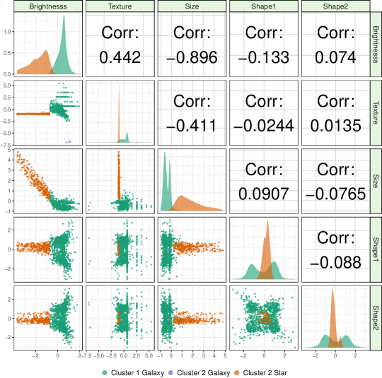
Figure 1: Scatterplots, univariate densities, and correlations of the transformed features of the SDSS data. The three colors correspond to the observed combinations of the two clusters specified by the $K=2$ $k_{m}$-means clustering and the true classification of each observation. Note that there are only four misclassifications, of galaxies (identified in blue).

Figure 1 displays the results of clustering in the transformed variable space are shown in the scatterplot matrix of Figure 1. (Here, color indicates membership in the final grouping from $k_{m}$-means, with shading corresponding to the observation’s true classification.)

TABLE I: Confusion matrix of the $k_{m}$-means (also $k$-POD) groups versus the true classes in the SDSS dataset.

Group	Stars	Galaxies
1	287	0
2	4	1216

Further, Table I provides a confusion matrix or cross-tabulation of the frequency of stars and galaxies classified in each $k_{m}$-means (or $k$-POD) group. If one considers the clusters as classifying stars and galaxies, only $4$ galaxies are misclassified. Further, every galaxy (and therefore every observation) with missing values is correctly classified. In this case, $k$-means clustering on only the complete observations results in an identical partition when comparing the grouping of only the complete observations but using $k_{m}$-means on the entire datasets. Thus, for these data, $k_{m}$-means is able to correctly cluster the incomplete observations, but that the inclusion of the incomplete observations has no effect on the clustering of the complete observations. Given that the incomplete observations make up a small percentage of the larger of the two clusters, this lack of a difference in class assignments is not unexpected.

The performance of $k_{m}$-means (and $k$-POD) is much better than that of any of the methods reported in Figure 1a of [16], where the best performer for $K=2$ had $AR\approx 0.2$. While we are unable to identify the reasons for the poorer performance reported in that paper, it is probable that our transformation to remove skewness and subsequent scaling may have had an important role in our better performance. Despite the transformations, it is clear that the features are not independent. There is clear separation between the two clusters in both brightness and size, which are strongly negatively correlated. Thus other approaches to clustering may also be worth pursuing for this dataset. However, this dataset offers a valuable illustration of $k_{m}$-means and indicates promise. We now proceed to evaluate the performance of $k_{m}$-means in several large-scale simulation experiments.

III-B Simulation Studies

III-B1 Experimental Framework

We thoroughly evaluated the $k_{m}$-means algorithm on a series of experiments encompassing different missingness mechanisms, clustering complexities, dimensions, numbers of clusters, proportions of missing values, and missingness mechanisms. We discuss these issues next.

Clustering Complexity of Simulated Datasets

The $k_{m}$-means algorithm inherently assumes data from homogeneously and spherically dispersed groups, so we restricted our attention to this framework. Within this setting, we simulated grouped data of different clustering complexities as measured by the generalized overlap measure and implemented in the C package CARP [54] or the R package MixSim [55], which is what we used in this paper. The generalized overlap (denoted by $\mathring{\omega}$ here) is a single-value summary of the pairwise overlap [56] between $K$ groups and is defined as $(\omega^{(1)}-1)/(K-1)$, where $\omega^{(1)}$ is the largest eigenvalue of the matrix of pairwise overlaps between the groups. $\mathring{\omega}$ takes higher values for greater overlap between groups (i.e., when there is higher clustering complexity) and lower values when the groups are well-separated. We simulated clustered data of different dimensions ($p$), different numbers of groups ($K$), different sample sizes ($n$) and different proportions ($\lambda$) of incomplete records. For each $(K,n,p,\lambda,\mathring{\omega})$, we considered four different mechanisms of missingness which led to the incompleteness of the records, as discussed next.

Missingness Mechanisms

Missing data are traditionally categorized into one of three different types: missing completely at random (MCAR), missing at random (MAR), and not missing at random (NMAR) [17]. For MCAR data, the probability that an observation record is missing a feature measurement depends neither on the observed values nor on the value of the missing data point. To simulate MCAR data, we randomly removed data independent of dimension and cluster. On the other hand, under MAR, the probability that an observation has a missing coordinate may depend on the observed values, but not on the true values of the missing data point. To simulate data under the MAR mechanism, we followed [32] in randomly removing data in only $40\%$ of the dimensions, leaving the other features completely observed. Note that in order to obtain a specific overall proportion $\lambda$ of missing data, the proportion of data missing in the partially observed dimensions will be higher – in our case $2.5\lambda$. When the probability that a value is missing depends on its true value, we say that the data are NMAR. We considered two different mechanisms for NMAR, namely NMAR1 for data that are MCAR but only in specified clusters, and NMAR2 that follows [32] in missing the bottom quantiles of each dimension in specified clusters. As with the MAR scenario, a higher proportion of data than $\lambda$ had to be removed in the partially observed groups to obtain the desired overall proportion of missing data.

Our experimental setup thus had a multi-parameter setup, with values as per Table II.

TABLE II: Values for each parameter used in simulation study.

Parameter	Values
# groups $(K)$	$4,7$
# observations $(n)$	$500,1000,5000$
Dimension $(p)$	$5,10$
Missing proportion $(\lambda)$	$0.05,0.1,0.2,0.3$
Overlap $(\mathring{\omega})$	$0.001,0.01,0.05$
Missingness mechanism	MCAR, MAR, NMAR1, NMAR2

The CARP and MixSim packages afford the possibility of providing general assessments of clustering performance in different settings. Therefore, for each of $(K,n,p,\lambda,\mathring{\omega})$ and missingness mechanism, we generated 50 synthetic datasets within the given experimental paradigm in order to assess performance. Thus, our simulation consisted of a total of 28,800 simulated datasets.

Additional details regarding implementation

We first compared performance of $k_{m}$-means with $k$-POD (through its R package kpodcluster) because both $k_{m}$-means and $k$-POD are geared towards optimizing (1) so can provide a direct comparison. We compared performance of the two algorithms for the case when $K$ is known in terms of execution speed, as well as (and more importantly) clustering efficacy measured in terms of $AR$. $k$-POD is naturally slower than $k_{m}$-means, due to its repeated application of the $k$-means algorithm at each iteration. Therefore, we used $100Kp$ initializations for $k_{m}$-means but only $5$ initializations for $k$-POD. The performance gains for $k_{m}$-means from using $100Kp$ initializations rather than $5$ initializations of $k_{m}$-means are in most cases minimal, and the use of unequal numbers of initializations across methods reflects how each would most likely be used in practice (with $k$-POD being used with a number of initializations that make it practical to apply.) We also evaluated performance of our modified jump statistic in deciding $K$.We chose our candidate $K$s to be in the set $\{1,2,\ldots,2K_{\bullet}\}$ where $K_{\bullet}$ was the true $K$ under which the particular simulated dataset was obtained. We restricted our use of the jump statistic estimator to $k_{m}$-means because the slower performance of $k$-POD makes application of $k$-POD for each candidate $K$ to be too computationally onerous to evaluate. We now report and discuss performance.

III-B2 Results

We first discuss performance of $k_{m}$-means and $k$-POD when $K$ is known and follow with clustering performance with $k_{m}$-means for when $K$ is unknown and estimated using our modified jump statistic.

Performance with Known $K$

We evaluate performance of $k_{m}$-means and $k$-POD in terms of execution time, initialization and clustering performance.

Execution Times:

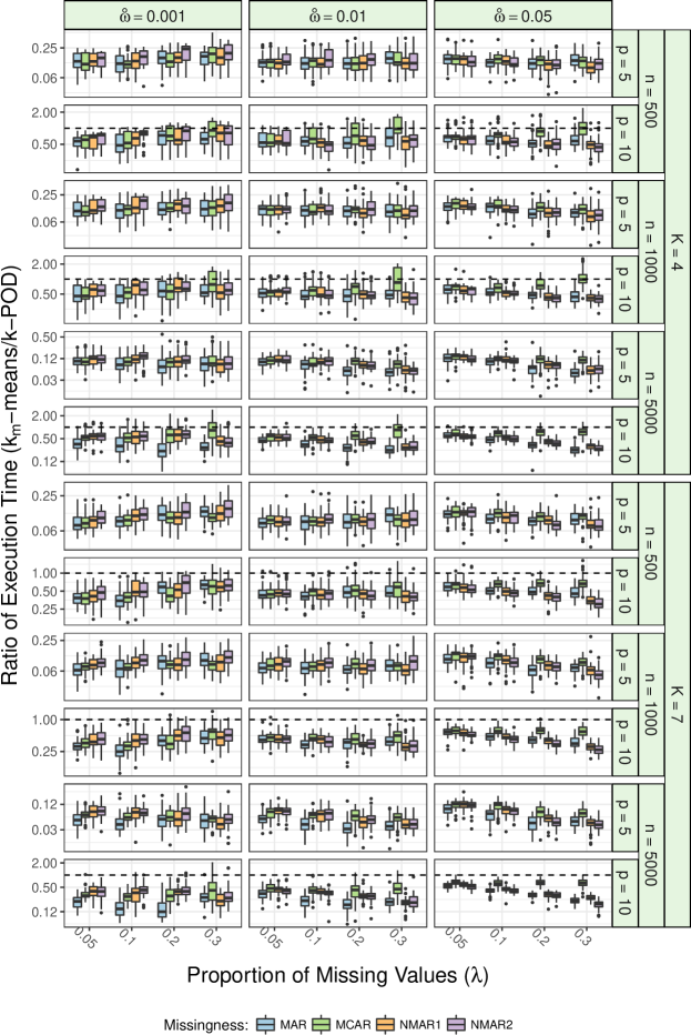
Figure 2: Ratio of execution times between $k_{m}$-means with $100Kp$ initializations each and $k$-POD with 5 initializations each for 50 simulated data sets in each simulation setting. The semi-solid line at 1 on the vertical axis is the point above and below which $k_{m}$-means takes more and less time, respectively, than $k$-POD.

Figure 2 displays the ratio of the execution times of $k$-POD and $k_{m}$-means, with known $K$. Even though $k_{m}$-means uses a far greater number of initializations (on the scale of $20kp$), it is in nearly all cases at least as fast as $k$-POD. Paired $t$-tests of the execution times show that $k_{m}$-means is significantly faster at an $\alpha=0.05$ level in all but two settings. Much of this difference can be attributed to the efficiency of the algorithms. In essence, for each initialization, $k$-POD must perform an entire $k$-means routine at each iteration, whereas $k_{m}$-means handles missing data within one $k$-means routine. Thus, with the exception of some special cases discussed in Section 3, one would expect $k_{m}$-means to be more efficient. (Note, however, that in these few cases, $k_{m}$-means would still have been faster if both $k_{m}$-means and $k$-POD were to have been run with the same number of initializations. Indeed, Figure S-3 which reports the per-initialization run relative gain of $k_{m}$-means over $k$-POD also supports this conclusion.)

Initialization: As described in Section II-C, Figures S-1a and S-1b respectively display the execution times and performance of our $k_{m}$-means algorithm when initialized using $\delta_{i,\mathcal{C}_{k}}^{2}$- and $\tilde{\delta}_{i,\mathcal{C}_{k}}^{2}$-weighting for selected settings. In general, initialization done using $\tilde{\delta}_{i,\mathcal{C}_{k}}^{2}$-weighting leads to faster clustering than that when using $\delta_{i,\mathcal{C}_{k}}^{2}$-weighting. In terms of final clustering performance, $\tilde{\delta}_{i,\mathcal{C}_{k}}^{2}$-weighting leads to better results than $\delta_{i,\mathcal{C}_{k}}^{2}$-weighting. This improved speed and performance is most pronounced in the case of lower $K$. In the few settings where $\delta_{i,\mathcal{C}_{k}}^{2}$-weighting is marginally better on average, the $AR$s for those clusterings are more widely-dispersed. It is interesting to note that of the two NMAR methods, clusterings on NMAR2 data are more accurate within each weighting relative to NMAR1. In this paper, we only report results from $k_{m}$-means using the $\tilde{\delta}_{i,\mathcal{C}_{k}}^{2}$-weighting.

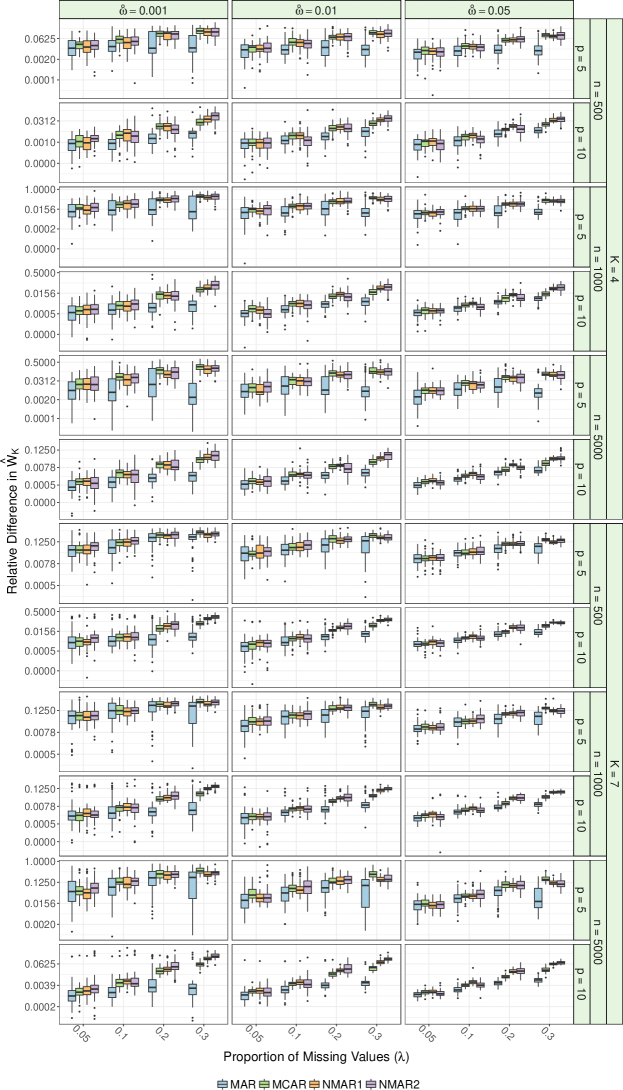
Figure 3: Relative difference in optimized objective function $\hat{\mathcal{W}}_{K}$ obtained using $k$-POD and $k_{m}$-means for 50 simulated data sets in each simulation setting.

Overall Comparisons: Figure 3 provides the relative decrease in the optimized $\hat{\mathcal{W}}_{K}$ upon using $k_{m}$-means over the $k$-POD algorithms. In general, the optimization improves more with deviations from MCAR as well as with increasing proportions of missing observations. This, despite $k_{m}$-means’ execution times that are a fraction of the $k$-POD execution times (Figure 2). Thus, in terms of optimizing  (1), $k_{m}$-means is uniformly a better

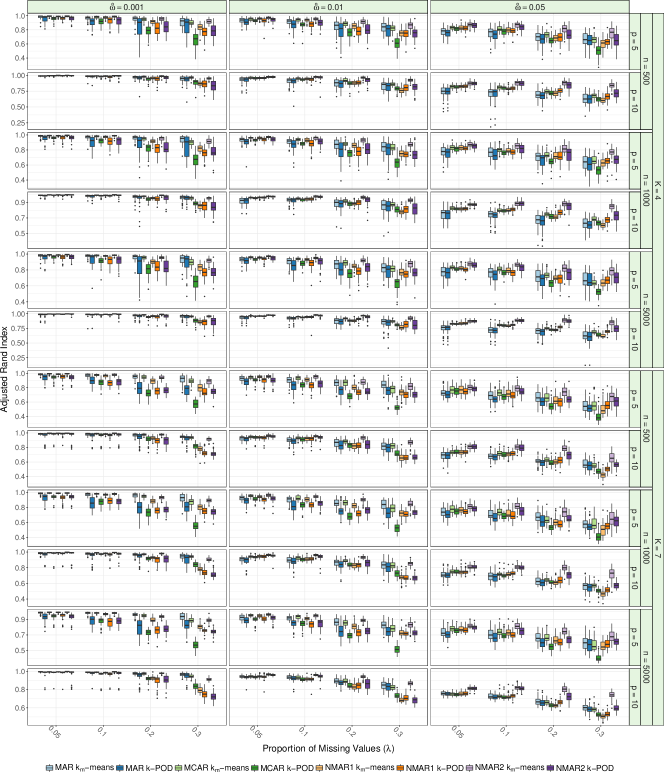
Figure 4: Adjusted Rand Index (AR) for $k_{m}$-means and $k$-POD for 50 simulated data sets in each simulation setting.

performer than $k$-POD. Figure 4 summarizes clustering performance in terms of $AR$ for each setting. Excluding NMAR1 data, $k_{m}$-means performs at least as well as $k$-POD, and significantly better as per one-sided paired t-tests in all but 5 settings. However, $k$-POD is the better performer in the NMAR1 cases with moderate to high clustering complexity (overlap) and with larger proportions of missing observations. We hypothesize that that is because the NMAR1 mechanism with large proportions of incomplete records and higher overlap results in unbalanced designs and estimated non-spherical clusters: in such a scenario, optimizing (1) may not be synonymous with finding the best clustering. This hypothesis is supported by Figure 3 that indicates that the terminal (local minimum) value obtained by $k_{m}$-means is lower than that obtained by $k$-POD. Further, the difference in execution times between the two methods for MCAR data shrinks as the proportion of incomplete records increases. As expected, performance for both methods suffers with increasing proportion of missing data or clustering complexity, but both methods perform admirably even outside of MCAR data. Finally, we note that the higher number of initializations used for $k_{m}$-means can not explain its superior performance over $k$-POD: Figure S-4 shows very similar results when only 5 initializations were used for both methods.

Estimating $K$ via the modified jump statistic

Because of the slower performance of $k$-POD, we only evaluate performance using $k_{m}$-means in this section. Figure 5 shows that the jump statistic often correctly estimates $K$, but underestimates it in more difficult cases, particularly with larger $K$. Errors are most strongly correlated with the proportion of missing data and cluster overlap, with poor estimation of $K$ when $K$, $\mathring{\omega}$, and $\lambda$ are at their highest values. There is noticeable difficulty in estimating $K$ in MAR data at $K=7$, but in each case, results improve with increasing $n$. (Recall that MAR data is missing significant proportions of values in selected features.)

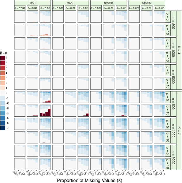
Figure 5: Difference between estimated number of clusters ($\hat{K}$) by the modified jump statistic and the true number of simulated clusters ($K$) for 50 simulated data sets in each simulation setting.

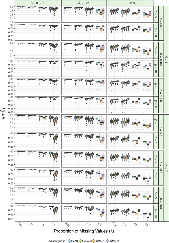
Figure 6: Adjusted Rand Indices ($AR(\hat{K})$) from $k_{m}$-means clusterings using the Jump-estimated number of clusters $\hat{K}$ for 50 simulated data sets in each simulation setting.

When data are heavily missing in this exact manner, but the partially observed features are known to be of importance, it may be more appropriate to use the soft constraints approach of [26]. We also observe a tendency to underestimate $K$ in each NMAR setting. This is to be expected, possibly even desired, because the NMAR settings may end up removing the majority of the values in clusters selected to be partially observed. Particularly as the overlap between clusters increases, it is not surprising that the jump estimator would underestimate $K$, and instead assign to nearby clusters the remaining observations with high proportions of missing values. Thus, we see limited improvement in $\hat{K}$ as $n$ increases in the NMAR settings. Figure 6 plots the $AR$ of the final clusterings using $\hat{K}$ and confirms our observations drawn from Figures 4 and 5. The observed $AR$s using $\hat{K}$ tend to be less than or equal to the $AR$ obtained using $K_{\bullet}$ but the differences are not large, with $AR\approx 1$ for lower values of $\mathring{\omega}$ and $\lambda$. We also see that in many cases, the $AR$ value for NMAR1 data is lower than those from other types of missingness. This can be traced back to the tendency to underestimate $K$ in NMAR1 data in particular.

III-B3 Comparison with Imputation Methods

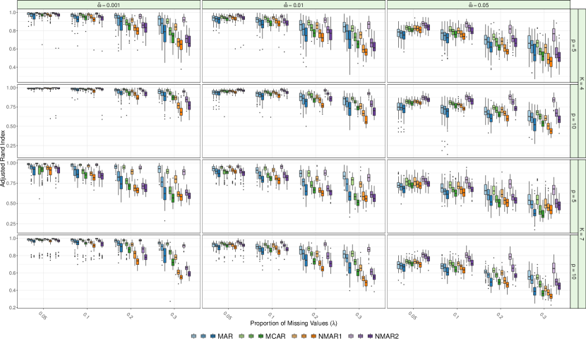
Figure 7: Performance of imputation methods and $k_{m}$-means on different simulation settings with known $K$ and for $n=500$. For each missingness mechanism in the figure, the light shades depict $k_{m}$-means while the medium and dark shades are for Amelia- and mice-imputed $k$-means groupings.

We have also, at the helpful suggestion of the Editor, provided a somewhat more limited comparison with two imputation methods. Our comparisons were only limited in that they were done for datasets with $n=500$ simulated records and known $K$ but having all the other simulation settings of Section III-B1. We compared $k_{m}$-means with two popular imputation methods Amelia [21] and and mice [22], both of which are implemented in R packages having the same respective names. Both methods draw imputations of the missing values. Amelia uses the Expectation-Maximization algorithm [57] on multiple bootstrapped samples of the original incomplete data to obtain estimates of the complete-data parameters, and then uses these bootstrapped estimates to replace the missing values with imputed values. On the other hand, mice draws imputations of the missing data points using chained equations.

For both imputation methods, we used the default settings to obtain imputed values for the missing observations and then used $k$-means on the results. Figure 7 shows the clustering performance of both imputation methods relative to $k_{m}$-means. We see a consistent improvement in accuracy of clustering using km-means with the largest difference in AR observed when the censoring methods stray further from assumptions made in Amelia and mice, for instance in the NMAR2 case, and also as the proportion of missing values increases. This deficiency of the imputation methods is not surprising because neither method directly uses the inherent grouped structure of the data and only provides imputations based on an overall (even though sophisticated) view of the data. Clustering algorithms are then used on the filled-in data values.

Our large-scale simulation experiments show that our $k_{m}$-means algorithm performs well over several different cluster sizes, missingness mechanisms, and proportions of missing values. Our modified jump statistic is also effective in selecting the number of groups. We now apply our methods to identify the kinds of activation in a finger-tapping experiment.

IV Identifying kinds of activation in a finger-tapping experiment

TABLE III: Number of voxels recording values in each replication in the fMRI experiment.

replication	1	2	3	4	5	6	7	8	9	10	11
# voxels	2103	2413	2666	1731	2378	1543	2583	2408	1834	894	1251

Functional magnetic resonance imaging (fMRI) is a noninvasive tool used to determine cerebral regions that are activated in response to a particular stimulus or task [58, 59, 60, 61]. The simplest experimental protocol involves acquiring images while a subject is performing a task or responding to a particular stimulus, and relating the time course sequence of images (after correction and pre-processing) to the expected response to the input stimulus [62, 63]. However, there are concerns about the inherent reliability and reproducibility of the identified activation [64, 65, 66]. [67] illustrates an example of differing activation maps obtained over twelve different sessions, where the same subject performed a simple finger-tapping task in each session. We seek to combine activation maps across each experiment to help understand the nature of brain activation in this experiment. It would be advantageous to have the ability to incorporate results from different fMRI studies without the need to re-analyze each experiment. Next, we show that this problem can be cast as an incomplete-records clustering problem.

Our data set for this experiment is from a left-hand finger-tapping experiment of a right-hand-dominant male and was acquired over twelve regularly-spaced sessions over the course of two months. Each data set was preprocessed and voxel-wise $Z$-scores were obtained that quantified the test statistic under the hypothesis of no activation at each voxel. The $Z$-scores from each session were thresholded using cluster-thresholding methods [68]. Because of concerns that the normally-right-hand-dominant male subject may have been inadvertently tapping his right hand fingers [67], the activation statistics for one session were dropped from our study. Thus, there are a total of eleven replicated test statistics. Our interest is then in classifying the voxels using their corresponding activation test statistics. Note that because of the thresholding, activation statistics are not available across all replicates. Table III lists the number of voxels above thresholding at each replication. There are 2827 total voxels that were identified as activated in at least one session, with a maximum of five missing values across replications. There are only $156$ voxels without any missing values. Thus, our goal is to cluster voxels based on the $Z$-scores of eleven replications, where incomplete records arise because, after thresholding, not all replications have a $Z$-score for each voxel. The use of $Z$-scores and assumption of independence over replications because of the substantial time between any two sessions makes this an ideal case for the assumption of homogeneous spherical dispersions for each sub-population of voxels.

As before, we run the $k_{m}$-means algorithm to termination, with $100p\max(K,10)$ initializations using the methods in Section II-C, for $K=1,2,\ldots,20$. The jump statistic identified the three-groups solution as the optimal partitioning. The resulting groups are displayed in Figure 8 separately, for each of the eleven

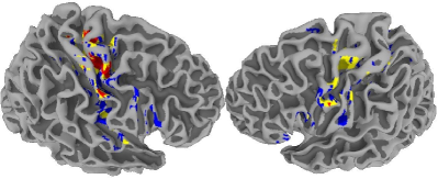
(a)

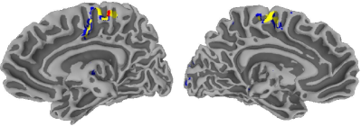
(b)

Figure 8: Regions of activation detected from voxels in eleven replications of an fMRI study.

experiments. The first group (denoted by red) consists of 235 voxels whose average mean $Z$-score is 10.31, the second (yellow) group has 965 voxels with average mean $Z$-score 6.83, and the third (blue) group includes 1627 voxels with an average mean $Z$-score of 4.96. The first group is where the activation is most emphatic and is almost entirely in the right primary motor cortex (M1), the ipsi- and contra-lateral pre-motor cortices (pre-M1), and the supplementary motor cortex (SMA). The other two groups of voxels represent two different kinds of milder activation and are primarily located in the right pre-SMA, and interestingly also in the left M1, pre-M1, and the SMA. This last observation is an interesting finding and is suggestive that activation in a right-hand dominant male is also associated in the left hemisphere of the brain even when it is the non-dominant hand that is active in performing a task. It is important to note that following a whole data strategy in this experiment would not have been able to identify this additional finding because almost all the 156 voxels that have non-thresholded $Z$-scores for all eleven replications (that is, having no missing values) are in the right hemisphere. Our application here also demonstrates an important approach to amalgamating the results from different fMRI activation studies.

V Discussion

We have extended the Hartigan-Wong $k$-means clustering algorithm to the case for datasets that have incomplete records. We do so by by defining a (partial) distance measure and objective function that ignores missing feature values. The modified objective function necessitates adapting [38]’s algorithm to account for incomplete records. We call the resulting algorithm $k_{m}$-means. We also provide modifications to the $k$-means++ initialization method and the jump statistic for estimating the number of clusters. C code implementing our methods is available at https://github.com/maitra/km-means. Our development represents an intuitive addition to the body of work seeking to avoid discarding partially observed data or imputing data. Simulations show this is an efficient and effective method for handling missing values, and application to astronomical data yielded results in line with expectations. The $k_{m}$-means approach was also valuable in the analysis of fMRI data, where the vast majority of observations (voxels) were treated as partially observed, and located in the same area. Our proposed methods in this paper thus provide a practical approach to $k$-means-type clustering in the presence of incomplete observations.

There are a number of issues that might benefit from further attention. In the context of $k_{m}$-means, there is a need for more research into initialization schemes for partially observed data. In addition to considering weighting schemes such as $\delta_{i,k}^{2}$ and $\tilde{\delta}_{i,k}^{2}$, alternative methods for choosing the initial center, $\hat{\bm{\mu}}_{1}$, may also lead to improved results. For example, we may limit $\hat{\bm{\mu}}_{1}$ to only completely observed data, or assign weights for choosing $\hat{\bm{\mu}}_{1}$ proportional to how many observed values each $\bm{X}_{i}$ has. Early results indicate each of these strategies lead to comparable results in most cases. The use of $k$-means and Euclidean distances for applications such as in the case of clustering of GRBs [18, 20] is not always appropriate. Therefore, appropriate adjustments are required for handling non-spherically dispersed groups of data or datasets with unequal variances. However, there is scope for optimism because, as pointed out by J. Bezdek, (1) used the Euclidean norm, but the proofs would generally hold for any inner product norm leading to possibly hyper-ellipsoidal-shaped groups. Additionally, the derivations would be fairly tractable even for the $\ell_{1}$ and $\ell_{\infty}$ norms. Finally, we note that it may also be possible to extend the general approach of this paper to data containing observations with repeated measures. Thus, while we have provided an efficient algorithm for finding homogeneous spherically-dispersed clusters in the case of incomplete records, several issues requiring further attention remain.

Supplementary Materials

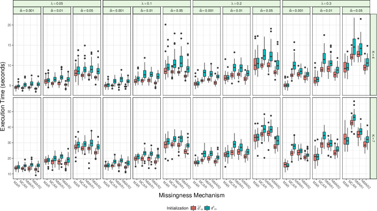
(a)

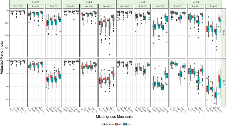
(b)

Figure S-1: (a) Execution times and (b) Adjusted Rand Indices of $k_{m}$-means using $\delta_{i,\mathcal{C}_{k}}^{2}$- and $\tilde{\delta}_{i,\mathcal{C}_{k}}^{2}$-weighting for initializations. Only settings with $p=10$ and $n=1,000$ are shown.

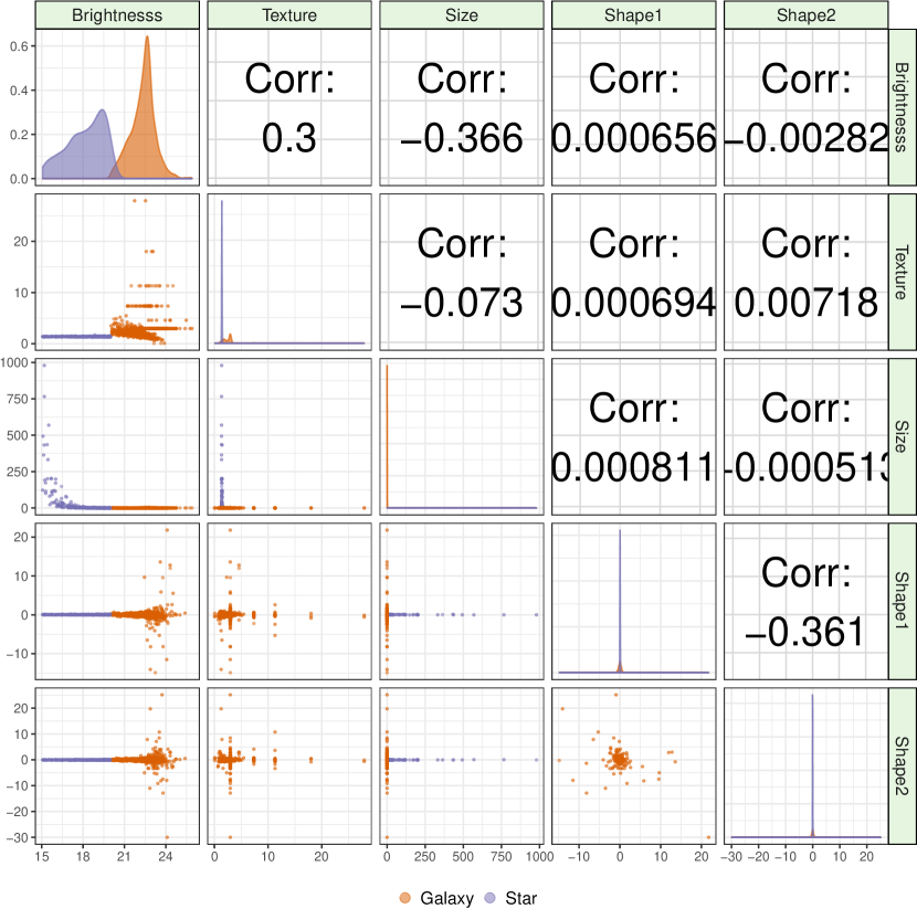
Figure S-2: Scatterplots, univariate densities, and correlations of the untransformed features of the SDSS data. The two colors correspond to the true classifications of each observation.

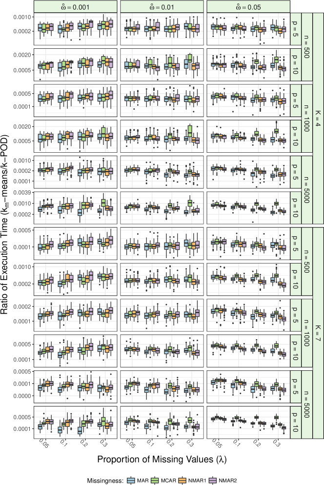
Figure S-3: Per-initialization execution time of $k_{m}$-means relative to $k$-POD.

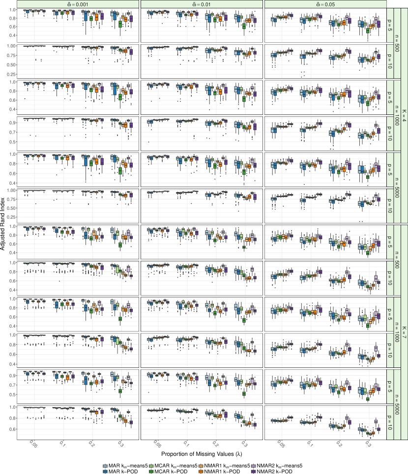
Figure S-4: Performance of $k_{m}$-means and $k$-POD when both methods were initialized 5 times.

References

- [1] C. D. Michener and R. R. Sokal, “A quantitative approach to a problem in classification,” Evolution, vol. 11, pp. 130–162, 1957.
- [2] A. Hinneburg and D. Keim, “Cluster discovery methods for large databases: from the past to the future,” in Proceedings of the ACM SIGMOD International Conference on the Management of Data, 1999.
- [3] R. Maitra, “Clustering massive datasets with applications to software metrics and tomography,” Technometrics, vol. 43, no. 3, pp. 336–346, 2001.
- [4] E. D. Feigelson and G. J. Babu, “Statistical Methodology for Large Astronomical Surveys,” in New Horizons from Multi-Wavelength Sky Surveys, ser. IAU Symposium, B. J. McLean, D. A. Golombek, J. J. E. Hayes, and H. E. Payne, Eds., vol. 179, 1998, p. 363.
- [5] A. K. Jain, “Data clustering: 50 years beyond k-means,” Pattern recognition letters, vol. 31, no. 8, pp. 651–666, 2010.
- [6] J. A. Hartigan and J. Hartigan, Clustering algorithms. New York: Wiley, 1975, vol. 209.
- [7] J. MacQueen et al., “Some methods for classification and analysis of multivariate observations,” in Proceedings of the fifth Berkeley symposium on mathematical statistics and probability, vol. 1, no. 14, Oakland, CA, USA., 1967, pp. 281–297.
- [8] S. Lloyd, “Least squares quantization in pcm,” IEEE transactions on information theory, vol. 28, no. 2, pp. 129–137, 1982.
- [9] J. R. Kettenring, “The practice of cluster analysis,” Journal of classification, vol. 23, pp. 3–30, 2006.
- [10] R. Xu and D. C. Wunsch, Clustering. NJ, Hoboken: John Wiley & Sons, 2009.
- [11] V. Melnykov and R. Maitra, “Finite mixture models and model-based clustering,” Statistics Surveys, vol. 4, pp. 80–116, 2010.
- [12] R. Maitra, V. Melnykov, and S. Lahiri, “Bootstrapping for significance of compact clusters in multi-dimensional datasets,” Journal of the American Statistical Association, vol. 107, no. 497, pp. 378–392, 2012.
- [13] W. Zhao, H. Ma, and Q. He, “Parallel k-means clustering based on mapreduce,” in IEEE International Conference on Cloud Computing. Springer, 2009, pp. 674–679.
- [14] S. Basu, M. Bilenko, and R. J. Mooney, “A probabilistic framework for semi-supervised clustering,” in Proceedings of the tenth ACM SIGKDD international conference on Knowledge discovery and data mining. ACM, 2004, pp. 59–68.
- [15] S. T. Roweis and L. K. Saul, “Nonlinear dimensionality reduction by locally linear embedding,” science, vol. 290, no. 5500, pp. 2323–2326, 2000.
- [16] K. L. Wagstaff and V. G. Laidler, “Making the most of missing values: Object clustering with partial data in astronomy,” in Astronomical Data Analysis Software and Systems XIV, vol. 347, 2005, p. 172.
- [17] R. J. Little and D. B. Rubin, Statistical analysis with missing data. New York: John Wiley & Sons, 2014.
- [18] S. Chattopadhyay and R. Maitra, “Gaussian-mixture-model-based cluster analysis finds five kinds of gamma ray bursts in the batse catalog,” Monthly Notes of the Royal Astronomical Society, vol. 469, no. 3, pp. 3374–3389, 2017. [Online]. Available: +http://dx.doi.org/10.1093/mnras/stx1024
- [19] R. J. Hathaway and J. C. Bezdek, “Fuzzy c-means clustering of incomplete data,” IEEE Transactions on Systems, Man, and Cybernetics, Part B (Cybernetics), vol. 31, no. 5, pp. 735–744, Oct 2001.
- [20] S. Chattopadhyay and R. Maitra, “Multivariate -Mixtures-Model-based Cluster Analysis of BATSE Catalog Establishes Importance of All Observed Parameters, Confirms Five Distinct Ellipsoidal Sub-populations of Gamma Ray Bursts,” Monthly Notes of the Royal Astronomical Society, 2018. [Online]. Available: +http://dx.doi.org/10.1093/mnras/stx1940
- [21] J. Honaker, G. King, M. Blackwell et al., “Amelia ii: A program for missing data,” Journal of statistical software, vol. 45, no. 7, pp. 1–47, 2011.
- [22] S. van Buuren and K. Groothuis-Oudshoorn, “mice: Multivariate imputation by chained equations in r,” Journal of statistical software, vol. 45, no. 3, 2011.
- [23] A. R. T. Donders, G. J. van der Heijden, T. Stijnen, and K. G. Moons, “Review: a gentle introduction to imputation of missing values,” Journal of clinical epidemiology, vol. 59, no. 10, pp. 1087–1091, 2006.
- [24] L. A. F. Park, J. C. Bezdek, C. Leckie, R. Kotagiri, J. Bailey, and M. Palaniswami, “Visual assessment of clustering tendency for incomplete data,” IEEE Transactions on Knowledge and Data Engineering, vol. 28, no. 12, pp. 3409–3422, Dec 2016.
- [25] M. Sarkar and T.-Y. Leong, “Fuzzy -means clustering with missing values,” in Proceedings of American Medical Informatics Association Annual Symposium (AMIA), 2001, pp. 588–592.
- [26] K. Wagstaff, “Clustering with missing values: No imputation required,” in Classification, Clustering, and Data Mining Applications, D. Banks, L. House, F. McMorris, P. Arabie, and W. Gaul, Eds. Springer, 2004, pp. 649–658.
- [27] K. Simiński, “Clustering with missing values,” Fundamenta informaticae, vol. 123, no. 3, pp. 331–350, 2013.
- [28] J. K. Dixon, “Pattern recognition with partly missing data,” IEEE Transactions on Systems, Man, and Cybernetics, vol. 9, no. 10, pp. 617–621, Oct 1979.
- [29] L. Himmelspach and S. Conrad, “Clustering approaches for data with missing values: Comparison and evaluation,” in 2010 Fifth International Conference on Digital Information Management (ICDIM), July 2010, pp. 19–28.
- [30] K. Simński, “Rough fuzzy subspace clustering for data with missing values.” Computing & Informatics, vol. 33, no. 1, 2014.
- [31] K. Simiński, “Rough subspace neuro-fuzzy system,” Fuzzy Sets and Systems, vol. 269, pp. 30–46, 2015.
- [32] J. T. Chi, E. C. Chi, and R. G. Baraniuk, “k-pod: A method for k-means clustering of missing data,” The American Statistician, vol. 70, no. 1, pp. 91–99, 2016.
- [33] D. R. Hunter and K. Lange, “A tutorial on mm algorithms,” The American Statistician, vol. 58, no. 1, pp. 30–37, 2004.
- [34] K. Lange, MM Optimization Algorithms. SIAM, 2016.
- [35] R Core Team, R: A Language and Environment for Statistical Computing, R Foundation for Statistical Computing, Vienna, Austria, 2017. [Online]. Available: https://www.R-project.org/
- [36] J. T. Chi and E. C. Chi, “kpodclustr: An r package for clustering partially observed data,” 2014, version 1.0. [Online]. Available: http://jocelynchi.com/kpodclustr
- [37] D. Arthur and S. Vassilvitskii, “k-means++: The advantages of careful seeding,” in Proceedings of the eighteenth annual ACM-SIAM symposium on Discrete algorithms. Society for Industrial and Applied Mathematics, 2007, pp. 1027–1035.
- [38] J. A. Hartigan and M. A. Wong, “Algorithm as 136: A k-means clustering algorithm,” Journal of the Royal Statistical Society. Series C (Applied Statistics), vol. 28, no. 1, pp. 100–108, 1979.
- [39] C. A. Sugar and G. M. James, “Finding the number of clusters in a dataset: An information-theoretic approach,” Journal of the American Statistical Association, vol. 98, no. 463, pp. 750–763, 2003.
- [40] R. Johnson and D. Wichern, Applied Multivariate Statistical Analysis. Pearson Education Limited, 2013.
- [41] R. Maitra and I. P. Ramler, “Clustering in the presence of scatter,” Biometrics, vol. 65, pp. 341 – 352, 2009.
- [42] H. Timm and R. Kruse, “Fuzzy cluster analysis with missing values,” in Fuzzy Information Processing Society-NAFIPS, 1998 Conference of the North American. IEEE, 1998, pp. 242–246.
- [43] R. Maitra, “Initializing partition-optimization algorithms,” IEEE/ACM Transactions on Computational Biology and Bioinformatics, vol. 6, pp. 144–157, 2009. [Online]. Available: http://doi.ieeecomputersociety.org/10.1109/TCBB.2007.70244
- [44] M. M. Astrahan, “Speech analysis by clustering, or the hyperphome method,” Stanford A I Project Memo, 1970.
- [45] G. W. Milligan, “The validation of four ultrametric clustering algorithms,” Pattern Recognition, vol. 12, pp. 41–50, 1980.
- [46] P. S. Bradley and U. M. Fayyad, “Refining initial points for K-Means clustering,” in Proceedings of the 15th International Conference on Machine Learning. Morgan Kaufmann, San Francisco, CA, 1998, pp. 91–99.
- [47] R. Ostrovsky, Y. Rabani, L. J. Schulman, and C. Swamy, “The effectiveness of lloyd-type methods for the k-means problem,” J. ACM, vol. 59, no. 6, pp. 28:1–28:22, Jan. 2013. [Online]. Available: http://doi.acm.org/10.1145/2395116.2395117
- [48] W. J. Krzanowski and Y. Lai, “A criterion for determining the number of groups in a data set using sum-of-squares clustering,” Biometrics, pp. 23–34, 1988.
- [49] G. W. Milligan and M. C. Cooper, “An examination of procedures for determining the number of clusters in a data set,” Psychometrika, vol. 50, no. 2, pp. 159–179, 1985.
- [50] G. Hamerly, C. Elkan et al., “Learning the k in k-means,” in NIPS, vol. 3, 2003, pp. 281–288.
- [51] D. Pelleg, A. W. Moore et al., “X-means: Extending k-means with efficient estimation of the number of clusters.” in ICML, vol. 1, 2000, pp. 727–734.
- [52] L. Hubert and P. Arabie, “Comparing partitions,” Journal of classification, vol. 2, no. 1, pp. 193–218, 1985.
- [53] L. M. John B. Burbidge and A. L. Robb, “Alternative transformations to handle extreme values of the dependent variable,” Journal of the American Statistical Association, vol. 83, no. 401, pp. 123–127, 198.
- [54] V. Melnykov and R. Maitra, “CARP: Software for fishing out good clustering algorithms,” Journal of Machine Learning Research, vol. 12, pp. 69 – 73, 2011.
- [55] V. Melnykov, W.-C. Chen, and R. Maitra, “Mixsim: An r package for simulating data to study performance of clustering algorithms,” Journal of Statistical Software, vol. 51, no. 12, pp. 1–25, 2012.
- [56] R. Maitra and V. Melnykov, “Simulating data to study performance of finite mixture modeling and clustering algorithms,” Journal of Computational and Graphical Statistics, vol. 19, no. 2, pp. 354–376, 2010.
- [57] A. P. Dempster, N. M. Laird, and D. B. Rubin, “Maximum likelihood for incomplete data via the EM algorithm (with discussion),” Jounal of the Royal Statistical Society, Series B, vol. 39, pp. 1–38, 1977.
- [58] P. A. Bandettini, A. Jesmanowicz, E. C. Wong, and J. S. Hyde, “Processing strategies for time-course data sets in functional mri of the human brain,” Magnetic Resonance in Medicine, vol. 30, pp. 161–173, 1993.
- [59] J. W. Belliveau, D. N. Kennedy, R. C. McKinstry, B. R. Buchbinder, R. M. Weisskoff, M. S. Cohen, J. M. Vevea, T. J. Brady, and B. R. Rosen, “Functional mapping of the human visual cortex by magnetic resonance imaging,” Science, vol. 254, pp. 716–719, 1991.
- [60] K. K. Kwong, J. W. Belliveau, D. A. Chesler, I. E. Goldberg, R. M. Weisskoff, B. P. Poncelet, D. N. Kennedy, B. E. Hoppel, M. S. Cohen, R. Turner, H.-M. Cheng, T. J. Brady, and B. R. Rosen, “Dynamic magnetic resonance imaging of human brain activity during primary sensory stimulation,” Proceedings of the National Academy of Sciences of the United States of America, vol. 89, pp. 5675–5679, 1992.
- [61] S. Ogawa, T. M. Lee, A. S. Nayak, and P. Glynn, “Oxygenation-sensitive contrast in magnetic resonance image of rodent brain at high magnetic fields,” Magnetic Resonance in Medicine, vol. 14, pp. 68–78, 1990.
- [62] K. J. Friston, P. Jezzard, and R. Turner, “Analysis of functional mri time-series,” Human Brain Mapping, vol. 1, pp. 153–171, 1994.
- [63] N. A. Lazar, The Statistical Analysis of Functional MRI Data. Springer, 2008.
- [64] R. Maitra, S. R. Roys, and R. P. Gullapalli, “Test-retest reliability estimation of functional mri data,” Magnetic Resonance in Medicine, vol. 48, pp. 62–70, 2002.
- [65] R. P. Gullapalli, R. Maitra, S. Roys, G. Smith, G. Alon, and J. Greenspan, “Reliability estimation of grouped functional imaging data using penalized maximum likelihood,” Magnetic Resonance in Medicine, vol. 53, pp. 1126–1134, 2005.
- [66] R. Maitra, “Assessing certainty of activation or inactivation in test-retest fMRI studies,” Neuroimage, vol. 47, pp. 88–97, 2009.
- [67] ——, “A re-defined and generalized percent-overlap-of-activation measure for studies of fMRI reproducibility and its use in identifying outlier activation maps,” Neuroimage, vol. 50, no. 1, pp. 124–135, 2010.
- [68] C.-W. Woo, A. Krishnan, and T. D. Wager, “Cluster-extent based thresholding in fMRI analyses: Pitfalls and recommendations,” Neuroimage, vol. 91, p. 412–419, 2014.