A tight-binding model for the band dispersion in rhombohedral topological insulators over the whole Brilluoin zone

Abstract

We put forward a tight-binding model for rhombohedral topological insulators materials with the space group $D^{5}_{3d}(R\bar{3}m)$. The model describes the bulk band structure of these materials over the whole Brillouin zone. Within this framework, we also describe the topological nature of surface states, characterized by a Dirac cone-like dispersion and the emergence of surface projected bulk states near to the Dirac-point in energy. We find that the breaking of the $R_{3}$ symmetry as one moves away from the $\Gamma$ point has an important role in the hybridization of the $p_{x}$, $p_{y}$, and $p_{z}$ atomic orbitals. In our tight-binding model, the latter leads to a band mixing matrix element ruled by a single parameter. We show that our model gives a good description of the strategies/mechanisms proposed in the literature to eliminate and/or energy shift the bulk states away from the Dirac point, such as stacking faults and the introduction of an external applied electric field.

I Introduction

Topological insulator (TI) materials have attracted a lot of attention over the recent years Hasan and Moore (2011); Qi and Zhang (2011); Hasan and Kane (2010). Their unusual metallic surface electronic structure on an inverted bulk band gap and the time reversal (TR) topological protection of these states, which forbids the backscattering, make TIs very fascinating materials Hasan and Moore (2011); Qi and Zhang (2011); Hasan and Kane (2010); Maciejko et al. (2010); Zhang et al. (2009); Mera Acosta et al. (2016). Due to the advances in synthesis techniquesEremeev et al. (2012) and their simple mathematical Liu et al. (2010) and computational modelingYang et al. (2012), Bi₂Se₃-like materials have been referred as the “hydrogen atom” of the 3DTIXia et al. (2009). These systems have been proposed as platforms for spintronic devices based on the control of induced magnetic moment direction Henk et al. (2012), surface barriersNarayan et al. (2014), and single-atom magnetoresistanceNarayan et al. (2015).

In addition to the metallic surface topological protected states in a insulating bulk, experiments find that Bi₂Se₃-like materials exhibit electronic scattering channels, attributed to the presence of bulk states near in energy to the Dirac pointHasan and Moore (2011); Zhang et al. (2009); Kim et al. (2011). These ubiquitous bulk states are believed to prevent the observation of the expected unusual electronic and transport properties governed by surface states in 3DTIsKim et al. (2011); Brahlek et al. (2015); de Vries et al. (2017).

First principles $GW$ calculations for surface states Yazyev et al. (2012); Förster et al. (2015, 2016) show that bulk states of Bi₂Se₃ thin films are shifted below the Dirac point, while this is not the case for Bi₂Te₃. In contrast, other bulk band structure calculations show that there is barely any energy separation between the Dirac point and the bulk valence band maximum Förster et al. (2016); Nechaev et al. (2013); Aguilera et al. (2013). This is at odds with recent experimental results de Vries et al. (2017) that, by investigating Shubnikov-de Haas oscillations in this material, showed the coexistence of surface states and bulk channels with high mobility.

In order to obtain insight on this problem and understand the experimentally observed magnetotransport properties of thin films of rhombohedral TI materials, one needs an effective model capable of describing both the topological surface states as well as the bulk ones over the whole Brillouin zone. In addition, the effective Hamiltonian has to account for the presence of external magnetic fields and be amenable to model disorder effects, which is beyond the scope of first principle methods. The main purpose of this paper is to put forward a tight-binding model that fulfills these characteristics.

Based on symmetry properties and $\bm{k}\cdot\bm{p}$ perturbation theory, Zhang and collaborators Liu et al. (2010) derived a Dirac-like Hamiltonian model describing the low energy band structure around the $\Gamma$-point of Bi₂Se₃-like 3DTIs. SubsequentlyMao et al. (2011), a tight-binding effective model has been proposed to describe the Brillouin of these systems, realizing both strong and weak TIs. However, the basis set used in such works fails to account for bulk states in the energy vicinity of the Dirac point and, hence, their effect on the electronic properties.

Here, we propose an effective tight-binding model that provides insight on the above mentioned bulk states close to the Fermi energy that potentially spoil the bulk-boundary duality. In the presence of disorder these states can mix with the surface ones, quenching the topological properties of the material. We also use our model to discuss some known mechanisms to cause an energy shift of the bulk states, such as, stacking faults Seixas et al. (2013) and applying an external electric field  Yazyev et al. (2010).

This paper is organized as follows. In Sec. II, we derive a tight-binding model for Bi₂Se₃-type 3DTI materials, that is based on their crystal structure symmetries and reproduces the bulk ab initio band structure calculations, thus describing the continuous bulk states near the Fermi level. In Sec. III we calculate the surface modes and discuss the microscopic origin of the bulk states in these materials. In Sec. IV we study mechanisms to eliminate and/or shift the bulk states below the Fermi surface. Finally, we present our conclusions in Sec. V. The paper also contains one Appendix containing a detailed technical description of the effective model and the tight-binding parameters for both Bi₂Se₃ andBi₂Te₃ compounds.

II TIGHT BINDING EFFECTIVE MODEL

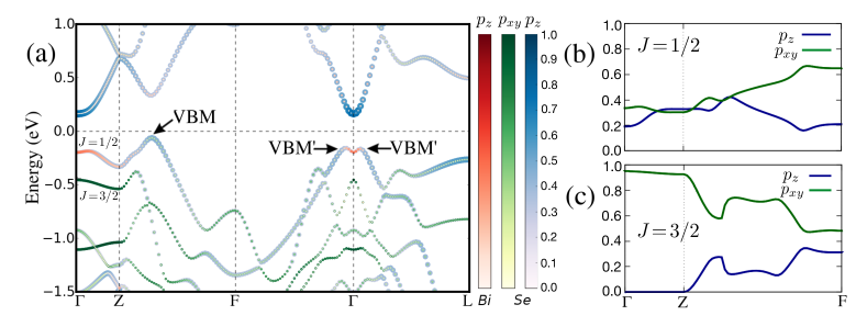
Figure 1: (Color online) (a) Bulk band structure of Bi₂Se₃. The color code stands for the projections of the $p_{z}$ Bi orbitals (red), $p_{x}p_{y}$ Se orbitals (blue), and $p_{z}$ Se orbitals (green) in the wave function. The maximum and local maxima of the valence band are denoted by VBM and VBM’, respectively. Panels (b) and (c) give the $p_{z}$ and $p_{x}p_{y}$ contributions of the $J=1/2$ and $J=3/2$ bands, respectively.

We begin this section by reviewing the key symmetry arguments that allow one to obtain a simple effective tight-binding model for Bi₂Se₃-like 3DTIs. Next, we present the ab initio electronic structure calculations on which our effective tight-binding model is based.

The crystalline structure of Bi₂Se₃-like 3DTIs is formed by Quintuple-Layers (QL) characterized by $D_{3d}^{5}(R{\overline{3}}m)$ point group symmetries Zhang et al. (2009). The Bi₂Se₃ QL unit cell is composed by two bismuth and three selenium atoms Zhang et al. (2009). The QL-QL interaction is weak, mainly ruled by the Van der Waals-like interaction Zhang et al. (2009); Liu et al. (2010); Seixas et al. (2013). This allows one to model each QL unit cell by a triangular lattice site. Following the approach presented in Ref. Liu et al., 2010, the Bi₂Se₃ hexagonal unit cell is conveniently described by three triangular lattice layers stacked in the $z$ direction, instead of considering three QL unit cells. This simple model preserves the symmetries of the $D_{3d}^{5}(R\overline{3}m)$ point group, namely: i) threefold rotation symmetry $R_{3}$ along the $z$ axis, ii) twofold rotation symmetry $R_{2}$ along the $x$ axis, iii) inversion symmetry $\mathcal{P}$, and iv) time-reversal symmetry $\mathcal{T}$.

It is well established Liu et al. (2010); Zhang et al. (2009) that the bulk wave function at the $\Gamma$ point can be accurately described by a set of few effective states $\{|\Lambda^{\tau}_{J},j_{z}\rangle\}$. Here, $\tau$ is the state parity, $J$ is the total angular momentum with projection $j_{z}$ on the $z$ axes, and $\Lambda$ labels the Bi and Se orbital contributions. We use these states to obtain an effective Hamiltonian that reproduces the bulk states of rhombohedral TIs calculated using ab initio methods.

The first-principle calculations are performed within the Density Functional Theory (DFT) frameworkCapelle (2006), as implemented in the SIESTA codeSoler et al. (2002), considering the on-site approximation for the spin-orbit couplingFernández-Seivane et al. (2006); Acosta et al. (2014). The Local Density Approximation (LDA)Perdew and Zunger (1981) is used for the exchange-correlation functional.

Figure 1 summarizes our ab initio results for Bi₂Se₃. The color code represents the contribution of the Bi and Se $p_{z}$ orbitals and the Se $p_{x}p_{y}$ atomic orbitals to the electronic structure. The main orbital contributions are associated with $p$ orbitals corresponding to $J=3/2,1/2$ and $j_{z}=\pm 3/2,\pm 1/2$ states (Fig. 1a). To conserve the total angular momentum the $|\Lambda^{\pm}_{3/2},\pm 3/2\rangle$ effective states must be a linear combination of $p_{x}$ and $p_{y}$ orbitals, whereas the $|\Lambda^{\pm}_{J},\pm 1/2\rangle$ states correspond to a linear combination of all $p$ orbitals (Fig. 1b and Fig. 1c). The symmetry properties of the $|\Lambda^{\tau}_{J},j_{z}\rangle$ states are discussed in Appendix A.

The bulk Valence Band Maximum (VBM) is located along the $Z\rightarrow F$ symmetry path, as shown in Fig. 1a. In addition, one finds two local maxima, denoted by VBM’, along the $F\rightarrow\Gamma$ and $\Gamma\rightarrow L$ lines, both close to the $\Gamma$-point. In line with previous resultsMao et al. (2011), we observe that both VBM and VBM’ have a strong $p_{z}$ Se orbital character. However, we find that the so far neglected $p_{x}p_{y}$ orbitals play a key role for an accurate description of the orbital composition of the valence band maxima, as we discuss below.

Along the $\Gamma\rightarrow Z$ symmetry line, the $R_{3}$ symmetry is preserved. Thus, the $|\Lambda_{1/2},\pm 1/2\rangle$ and $|\Lambda_{3/2},\pm 3/2\rangle$ effective states do not mix. In contrast, in the $\Gamma\rightarrow L$ and $\Gamma\rightarrow F$ paths the $R_{3}$ symmetry is broken. This allows for the hybridization of $p_{z}$ atomic orbitals with $p_{x}$ and $p_{y}$ ones. We find that this hybridization can be rather large, as clearly shown by Figs. 1b and 1c, where we present the Se orbital composition of the $J=1/2$ and $J=3/2$ bands along the Brillouin zone.

Since the valence band maxima do not belong to the $\Gamma\rightarrow Z$ symmetry line, their orbital composition is a superposition of all $p$ Se-atomic orbitals. As a consequence, a minimal Hamiltonian aiming to effectively describe VBM and VBM’ needs to take into account the states associated with the $p_{x}$ and $p_{y}$ orbitals, instead of including just the states with $p_{z}$ character Liu et al. (2010); Mao et al. (2011).

To calculate the surface electronic structure in the presence of surface projected bulk states, we consider a tight-binding model with eight states, namely, the $|\text{Se}^{-}_{1/2},\pm 1/2\rangle$ and $|\text{Bi}^{+}_{1/2},\pm 1/2\rangle$ states responsible for the band inversion, and $|\text{Se}^{-}_{3/2},\pm 3/2\rangle$ and $|\text{Se}^{+}_{3/2},\pm 3/2\rangle$ that dominate the most energetic $J=3/2$ band. Using this basis, we write the 8$\times$8 Hamiltonian:

$$\mathcal{H}(\bm{k})=\left(\begin{array}[]{cc}\mathcal{H}_{1/2}(\bm{k})&\mathcal{H}_{\rm int}(\bm{k})\\ \mathcal{H}_{\rm int}^{\dagger}(\bm{k})&\mathcal{H}_{3/2}(\bm{k})\\ \end{array}\right),$$ (1)

where $\mathcal{H}_{1/2}(\bm{k})$ is the standard 4$\times$4 Hamiltonian discussed in the literature Liu et al. (2010); Mao et al. (2011), that considers only $|{\rm Bi}^{+}_{1/2},\pm 1/2\rangle$ and $|{\rm Se}^{-}_{1/2},\pm 1/2\rangle$ states Our model introduces $\mathcal{H}_{3/2}(\bm{k})$, a 4$\times$4 Hamiltonian associated with the $|{\rm Se}^{-}_{3/2},\pm 3/2\rangle$ and $|{\rm Se}^{+}_{3/2},\pm 3/2\rangle$ states, and $\mathcal{H}_{\rm int}(\bm{k})$ the corresponding coupling term.

For a given total angular momentum $J$ the matrix elements in $\mathcal{H}(\bm{k})$ read

$$[\mathcal{H}(\bm{k})]_{ii^{\prime}}=\varepsilon_{ii^{\prime}}(\bm{k})\delta_{ii^{\prime}}+\sum_{\nu}\left(t^{ii^{\prime}}_{\bm{a}_{\nu}}e^{i\bm{k}\cdot\bm{a}_{\nu}}+t^{ii^{\prime}}_{\bm{b}_{\nu}}e^{i\bm{k}\cdot\bm{b}_{\nu}}\right),$$ (2)

where the states are labeled by $i=(\Lambda,J,\tau,j_{z})$, $\varepsilon_{ii}(\bm{k})$ are on-site energy terms, and $t^{ii^{\prime}}_{\bm{c}}=\langle{\bm{n}},\Lambda^{\tau}_{J},j_{z}|H|\bm{n}+{\bm{c}},\Lambda^{{}^{\prime}\tau^{\prime}}_{J^{\prime}},j_{z}^{\prime}\rangle$ are the corresponding nearest neighbor QL hopping terms, with $\bm{n}_{\nu}$ and $\tau$ indicating lattice site and orbital parity, respectively. Here ${\bm{c}}={\bm{a}}_{\nu}$ or ${\bm{b}}_{\nu}$, where $\pm\bm{a}_{\nu}$ stands for the 6 intra-layer nearest neighbor vectors of each triangular lattice, namely, ${\bm{a}}_{1}=(a,0,0),\bm{a}_{2}=(-a/2,\sqrt{3}a/2,0),\bm{a}_{3}=(-a/2,-\sqrt{3}a/2,0)$, while $\pm\bm{b}_{\nu}$ denotes the 6 inter-layer nearest neighbors vectors, ${\bm{b}}_{1}=(0,\sqrt{3}a/3,c/3),{\bm{b}}_{2}=(-a/2,-\sqrt{3}a/6,c/3),{\bm{b}}_{3}=(a/2,-\sqrt{3}a/6,c/3)$ with $a=4.14$ Å and $c=28.70$ Å Zhang et al. (2009).

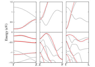
Figure 2: (Color online) Comparison between the DFT (gray solid lines) and the tight-binding model (red dotted lines) bulk band structure of Bi₂Se₃.

Exploring the system symmetries, we find constraints relating the nearest neighbors QL hopping terms $t^{ij}_{\bm{c}}$, thereby reducing the total number of possible hopping terms from 432 to 30 independent ones (see Appendix A). The corresponding 30 tight-binding parameters are determined by fitting the tight-binding model bulk band structure to the one calculated with DFT, shown in Fig 2. We present the complete Hamiltonian and provide more details on the fitting procedure in Appendix A.

The proposed Hamiltonian captures the low-energy ab initio band dispersion, even for $k$-points far from $\Gamma$, overcoming an intrinsic limitation of the ${\bm{k}}\cdot{\bm{p}}$ models proposed in the literature to describe the band inversion at the $\Gamma$ point. We show in the Appendix A how to reduce our model to a ${\bm{k}}\cdot{\bm{p}}$ Hamiltonian by taking the approximation $k\rightarrow\Gamma$ and relating, for instance, the hopping terms $t^{ii^{\prime}}_{\bm{a}_{\nu}}$ and $t^{ii^{\prime}}_{\bm{b}_{\nu}}$ to the perturbation theory parameters of Ref. Liu et al., 2010. The inclusion of additional bands does not affect the band inversion, for instance, the $J=3/2$ bands have much lower energies than the $J=1/2$ bands.

III Thin films

In this section we calculate the electronic band structure of rhombohedral TI thin films. We take the QLs parallel to the $xy$-plane and define the $z$-axis as the stacking direction. The thickness of the films is given in terms of $N_{\rm QL}$, the number of stacked QLs. The surface corresponds to the outermost QLs. The surface states correspond to the ones spatially localized in these QLs.

We modify the bulk tight-binding Hamiltonian defined in Eq. (1) to account for a finite number of layers. The slab Hamiltonian consists of intra- and inter-layer terms, namely Ebihara et al. (2012)

$$\mathcal{H}_{\rm slab}=\sum_{n=1}^{N_{\rm QL}}{c}^{\dagger}_{n}\mathcal{H}_{0}{c}_{n}+\sum_{n=1}^{N_{{\rm QL}}-1}\left({c}^{\dagger}_{n}\mathcal{H}_{z}{c}_{n+1}+\rm{H.c.}\right).$$ (3)

The basis is given by $|n,k_{x},k_{y},\Lambda^{\tau}_{J},j_{z}\rangle$ with corresponding creation (annihilation) operators given in compact notation by $c^{\dagger}_{n}$ ($c_{n}$). The intra-layer matrix elements read

$$[\mathcal{H}_{0}({\bm{k}})]_{ii^{\prime}}=\varepsilon_{i}({\bm{k}})\delta_{ii^{\prime}}+\sum_{\nu=1}^{6}t^{ii^{\prime}}_{\bm{a}_{\nu}}e^{i\bm{k}\cdot\bm{a}_{\nu}}.$$ (4)

The latter are similar to those of Eq. (2), but restricted to two-dimensions, namely, ${\bm{k}}=(k_{x},k_{y})$. In turn, the inter-layer term,

$$[\mathcal{H}_{z}]_{ii^{\prime}}=\sum_{\nu}t^{ii^{\prime}}_{\bm{b}_{\nu}},$$ (5)

provides the coupling between nearest neighbor QLs planes.

It is well established that a bulk band inversion occurs between states dominated by $p_{z}$ Se and Bi atomic orbitals with different parities Zhang et al. (2009). The four states $|\text{Se}^{-}_{1/2},\pm 1/2\rangle$ and $|\text{Bi}^{+}_{1/2},\pm 1/2\rangle$ form a good basis to describe the surface states at the $k$-points near the $\Gamma$ point Liu et al. (2010); Mao et al. (2011). However, similarly to bulk systems, this reduced basis also fails to correctly describe the bulk states close in energy to the Dirac point in thin Bi₂Se₃ films.

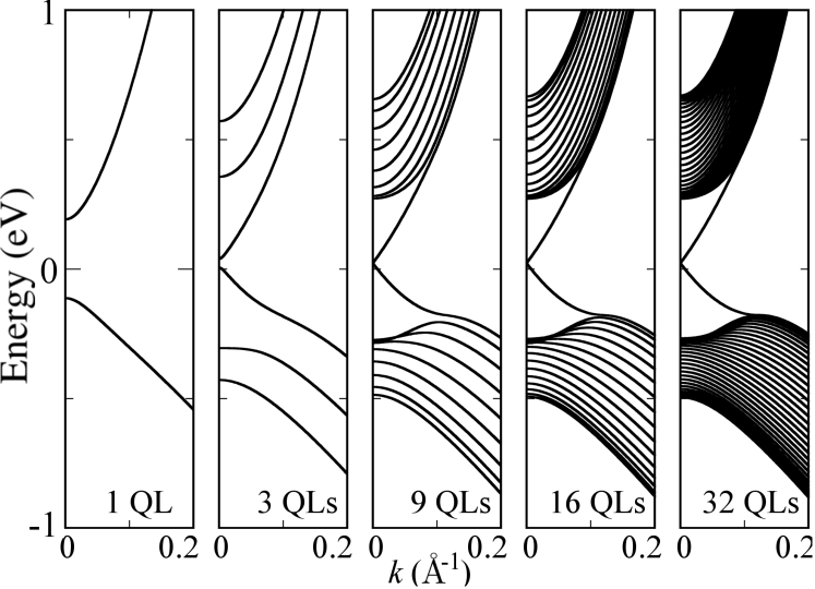
Figure 3: Band structure along the $\Gamma\rightarrow M$ symmetry line, without considering $J=3/2$-states, for different film thicknesses of Bi₂Se₃.

To better understand the importance of the $J=3/2$ states, let us first consider a thin film described by the Hamiltonian $\mathcal{H}_{1/2}({\bm{k}})$ projected out from $\mathcal{H}_{\rm slab}$. Figure 3 shows the finite size effects and how the band structure is modified by increasing $N_{\rm QL}$Ebihara et al. (2012). For $N_{\rm QL}\geqslant 3$ one clearly observes the appearance of surface states and the formation of a Dirac cone. For $N_{\rm QL}\gg 1$ the bulk band gap is recovered. We stress that without the $J=3/2$ states, the model does not show VBM bulk states close to the Fermi level, as expected from the analysis of bulk band structure (see, for instance, Fig. 1). Moreover, within this simple model the band structure close to the Dirac point along the $\Gamma\rightarrow K$ and $\Gamma\rightarrow M$ paths are identical, which is a rather unrealistic symmetry feature.

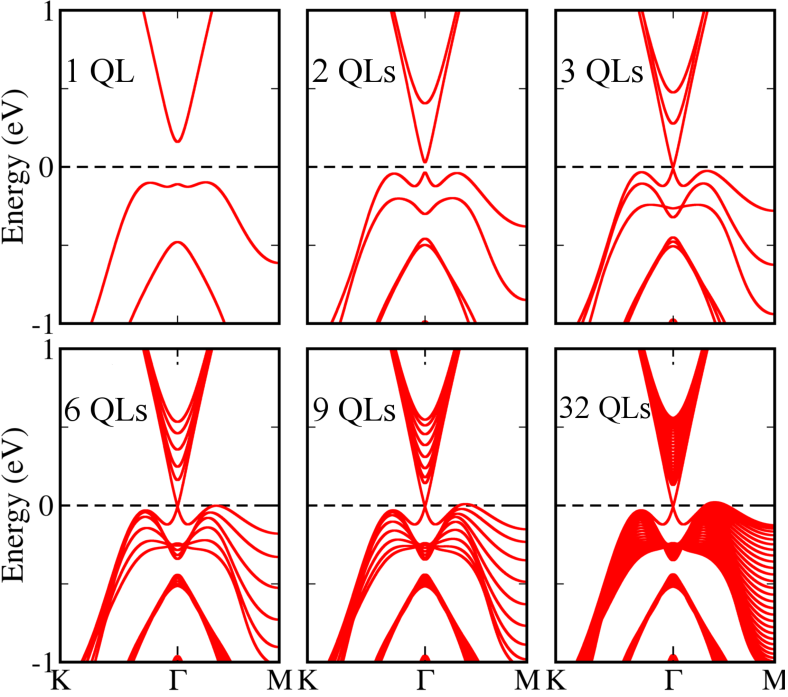
Figure 4: (Color online) Band structure of a Bi₂Se₃ thin film for different thickness values, $N_{\rm QL}=1,2,3,6,9,$ and 32, using our 8$\times$8 tight-binding effective model.

The $J=3/2$ states modify significantly the electronic band structure. Figure 4 summarizes the results we obtain for the 8$\times$8 total effective Hamiltonian, Eq. (1). Even for a few QLs, the shape of the surface band structure reproduces the qualitative behavior observed in the bulk LDA-DFT calculations. Figure 4 shows that as $N_{\rm QL}$ is increased, the Dirac cone is formed and bulk states appear in the vicinity of the Fermi level turning the system into a metal.

IV Application: Bulk states engineering

Several strategies have been proposed and used to suppress the scattering channels associated with the continuous bulk states, like for instance, alloy stoichiometry Zhang et al. (2011); Arakane et al. (2012); Ren et al. (2011); Abdalla et al. (2015), application of an external electric fieldYazyev et al. (2010), stacking faultsSeixas et al. (2013), and strainLiu et al. (2014); Park et al. (2015).

Let us now use the effective model put forward in the previous section to discuss some of these known strategies to shift the bulk band states away from the Dirac point energy, defined as $\varepsilon=0$.

Our analysis is based on the observation that the energy of the bulk states along the $\Gamma\rightarrow M$ symmetry path depends very strongly on the in-plane interaction between $|{\rm Se}^{-}_{1/2},\pm 1/2\rangle$ and $|{\rm Se}^{+}_{3/2},\pm 3/2\rangle$ states. We find that by increasing the matrix elements associated with the mixture of the above states the bulk states are shifted up in energy, as shown by Fig. 5.

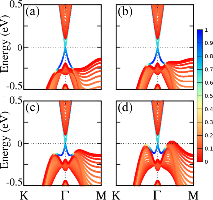
Figure 5: (Color online) Surface band structure for $N_{\rm QL}=20$ calculated using the eight bands effective model with hopping term (repulsion parameter) (a) $t^{ij}_{b}=1.2$ eV, (b) $t^{ij}_{b}=1.5$ eV, (c) $t^{ij}_{b}=1.8$ eV, and (d) $t^{ij}_{b}=2.1$ eV, where $i=(\mbox{Se}_{1/2}^{-},\pm 1/2)$, and $j=(\mbox{Se}_{3/2}^{+},\pm 3/2)$. The color code stands for the magnitude of the projection of the orbitals at the outermost (surface) QLs. Pure surface states are indicated by blue, whereas bulk states are depicted in red.

Hence, as previously proposed Abdalla et al. (2015), one way to engineer the VBM and VBM^′ states is by substituting the Se atoms by chemical elements that do not spoil the topological properties of the material and reduce the interaction between $|{\rm Se}^{-}_{1/2},\pm 1/2\rangle$ and $|{\rm Se}^{+}_{3/2},\pm 3/2\rangle$ states. This effect can be described by a simple model in terms of the direct modification of the matrix element $t^{ij}_{b}$ that mixes the $|{\rm Se}^{-}_{1/2},\pm 1/2\rangle$ and $|{\rm Se}^{+}_{3/2},\pm 3/2\rangle$ states. In fact, the band structures obtained for several values of $t^{ij}_{b}$ shown in Fig. 5 qualitatively describe the first-principles calculations for Bi₂(Se_1-xS_x)₃ alloys Abdalla et al. (2015).

Alternatively, the double degenerate surface-state bands due to the presence of two [111] cleavage surfaces in a slab geometry can be removed by applying a perpendicular electric field $E_{0}\hat{z}$ Yazyev et al. (2010). The Dirac cone associated with the surface at the highest potential energy can be shifted above the VBM, leading to a suppression of the scattering channels between the topologically protected metallic surface states and the bulk states. We describe this effect using our tight-binding effective model by modifying the on-site term $\varepsilon(\bm{k})\delta_{ij}$ in the inter-layer matrix elements associated with each QL. As a result, Eq. (4) becomes

$$[\mathcal{H}_{0}(k_{x},k_{y})]_{n,ij}=\tilde{\varepsilon}_{n}(\bm{k})\delta_{ij}+\sum_{\nu}t^{ij}_{\bm{a}_{\nu}}e^{i\bm{k}\cdot\bm{a}_{\nu}},$$ (6)

where $\tilde{\varepsilon}_{n}(\bm{k})=\varepsilon(\bm{k})+nceE_{0}/N_{QL}$, $n$ is the layer index, and $e$ is the electron charge. This simple approach captures the shift of the Dirac cone located at the surfaces corresponding to the QL with $n=N_{QL}$ and $n=0$. Figure 6a show the effect of an electric field of $E=5\times 10^{-3}$ V/Å  on a thin film of $N_{\rm QL}=9$.

Another band engineering strategy has been suggested by ab-initio atomistic investigations on the role played by extended defects, like stacking faults, on the structural and electronic properties of 3D topological insulators Seixas et al. (2013). In $R\overline{3}m$ structures the typical stacking is a ABCABC configuration, that is, each QL is rotated with respect to its adjacent QL by 120^o. When a QL is “removed” leading to a ACABCA, ABABCA, or ABCBCA stacking configuration, the defects is called an intrinsic stacking fault. The inter-QLs distance decreases as a consequence of these stacking faults, making the Van der Waals inter-QLs interaction weaker and changing the on-site potential of the QLs in which the structural defect is located Seixas et al. (2013). Thus, it is relatively easy to account for this effect within our model, namely, we rewrite the on-site energy and the inter band interaction as $\varepsilon_{n}(\bm{k})-\delta\varepsilon_{0}$ and $t^{ij}_{\bm{b}_{\nu}}-\delta t$.

Stacking faults nearby the surface layers of Bi₂Se₃ give rise to a positive energy shift of the bulk states with respect to their energy in a pristine systemSeixas et al. (2013). This shift is typically about 75 meV. Thus, we obtain a qualitative description of the stacking faults effect by fitting $\delta\varepsilon_{0}$ and $\delta t$ to the DFT results only for the QLs with this structural defect, see Fig. 6. Our simplified model and description allows for the study of thin films with a large number of QLs.

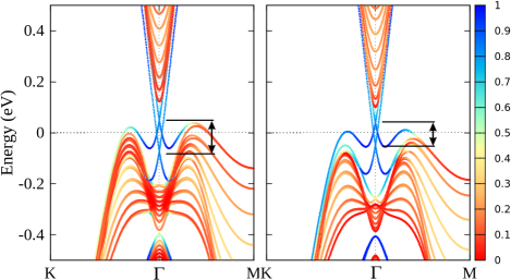
Figure 6: (Color online) Electric field (left) and stacking faults (right) effect of the band structure of a Bi₂Se₃ thin film of 9QLs. The splitting between the Dirac cones associated with different surfaces is represented by the arrow. The color code quantifies the surface/bulk character of the electronic states, see caption of Fig. 5.

V Conclusions

We have revisited the band structure calculations of rhombohedral topological insulators, both bulk and thin films, and investigated the occurrence of bulk states at the Fermi level. Based on ab initio calculations, we construct a simplified tight-binding model considering the states with angular momentum $J=1/2$ and $J=3/2$ and therefore, taking explicitly into account the $p_{x}p_{y}$ Se orbitals contributions.

Our model shows that the energy of bulk states near the Dirac-point is associated with a band mixing, which is mainly ruled by the hopping term between $p_{z}$ and $p_{x}p_{y}$ states. The valence band maximum appears in the symmetry path in which the $R_{3}$ symmetry is broken. In this situation, the $J=3/2$ states can mix with the $J=1/2$ ones.

We illustrate the versatility of our tight-binding model by studying some strategies to eliminate and/or shift the bulk states away from the Fermi surface. We show that the band structures obtained using our simple model reproduce qualitatively very well computationally costly ab initio calculations found in the literature.

In summary, we show that our simple effective model captures the main surface band structure features, allowing to explore strategies to perform a continuous bulk states engineering and opening the possibility to model disorder, which is ubiquitous in rhombohedral TIs and beyond the scope of ab initio calculations.

Appendix A Full effective Hamiltonian and model parameters

As discussed in the main text, the form of proposed effective Hamiltonian is obtained by considering symmetry arguments only, which allows one to address the complete family of rhombohedral materials. In turn, the model parameters are determined by fitting the electronic properties obtained from a given first principle calculation.

In this Appendix we discuss in detail the reasoning behind the construction of the model and present explicit expressions for the matrix elements of the resulting effective Hamiltonian. The Appendix presents also the model parameters for both Bi₂Se₃ and Bi₂Te₃ compounds.

Let us begin recalling that the effective Hamiltonian $\mathcal{H}({\bm{k}})$, Eq. (1) reads

$$\mathcal{H}(\bm{k})=\left(\begin{array}[]{cc}\mathcal{H}_{1/2}(\bm{k})&\mathcal{H}_{\rm int}(\bm{k})\\ \mathcal{H}_{\rm int}^{\dagger}(\bm{k})&\mathcal{H}_{3/2}(\bm{k})\\ \end{array}\right).$$ (7)

The states with effective angular moment $J=3/2$ are combination of two representations of the double group $D_{3d}^{5}(R3m)$. Therefore, we consider the states with defined representation:

$$\left|\Lambda^{\pm},\Gamma_{4}\right\rangle=\frac{1}{\sqrt{2}}\left(|\Lambda^{\pm}_{3/2},3/2\rangle+|\Lambda^{\pm}_{3/2},-3/2\rangle\right),$$ (8)

and

$$\left|\Lambda^{\pm},\Gamma_{5}\right\rangle=\frac{1}{\sqrt{2}}\left(|\Lambda^{\pm}_{3/2},3/2\rangle-|\Lambda^{\pm}_{3/2},-3/2\rangle\right).$$ (9)

The states $\{|\Lambda^{\tau}_{J},j_{z}\rangle\}$ are transformed by the symmetries operator as

1. Threefold rotation $R_{3}$:

   $$\left|\Lambda^{\pm},\Gamma_{4,5}\right\rangle\rightarrow -\left|\Lambda^{\pm},\Gamma_{4,5}\right\rangle,$$

   $$\left|\Lambda^{\pm},\pm 1/2\right\rangle\rightarrow e^{\pm\frac{i\pi}{3}}\left|\Lambda^{\pm},\pm 1/2\right\rangle.$$

2. Twofold rotation $R_{2}$:

   $$\left|\Lambda^{\pm},\Gamma_{4}\right\rangle\rightarrow \pm i\left|\Lambda^{\pm},\Gamma_{4}\right\rangle,$$

   $$\left|\Lambda^{\pm},\Gamma_{5}\right\rangle\rightarrow \mp i\left|\Lambda^{\pm},\Gamma_{5}\right\rangle,$$

   $$\left|\Lambda^{+},\pm 1/2\right\rangle\rightarrow i\left|\Lambda^{+},\mp 1/2\right\rangle,$$

   $$\left|\Lambda^{-},\pm 1/2\right\rangle\rightarrow -i\left|\Lambda^{-},\mp 1/2\right\rangle.$$

3. Inversion $\mathcal{P}$:

   $$\left|\Lambda^{\pm},\Gamma_{4,5}\right\rangle\rightarrow \pm\left|\Lambda^{\pm},\Gamma_{4,5}\right\rangle,$$

   $$\left|\Lambda^{\pm},\alpha\right\rangle\rightarrow \pm\left|\Lambda^{\pm},\alpha\right\rangle\quad\mbox{with}\quad\alpha=\pm 1/2.$$

4. Time reversal $\mathcal{T}$:

   $$\left|\Lambda^{\pm},\Gamma_{4,5}\right\rangle\rightarrow -\left|\Lambda^{\pm},\Gamma_{5,4}\right\rangle,$$

   $$\left|\Lambda,\pm 1/2\right\rangle\rightarrow \pm\left|\Lambda,\mp 1/2\right\rangle.$$

These symmetry transformations relate the hopping terms to each other, as shown for $t_{{\bm{c}}_{\nu}}^{11}=\langle 0,{\rm Bi}^{+}_{1/2},1/2|H|{\bm{c}}_{\nu},{\rm Bi}^{+}_{1/2},+1/2\rangle$ in Table 1.

Table 1: Symmetry operations on the hopping matrix element $t_{{\bm{c}}_{\nu}}^{11}=\langle 0,{\rm Bi}^{+}_{1/2},+1/2|H|{\bm{c}}_{\nu},{\rm Bi}^{+}_{1/2},+1/2\rangle$, where ${\bm{c}}_{\nu}={\bm{a}}_{\nu}$ or ${\bm{b}}_{\nu}$, and $\nu=1,2$ or 3. (For completeness, we recall that $t_{{\bm{c}}_{\nu}}^{22}=\langle 0,{\rm Bi}^{+}_{1/2},-1/2|H|{\bm{c}}_{\nu},{\rm Bi}^{+}_{1/2},-1/2\rangle$.)

	$t_{a_{1},b_{1}}^{11}$	$t_{{a}_{2},b_{2}}^{11}$	$t_{{a}_{3},b_{3}}^{11}$	$t_{-a_{1},-b_{1}}^{11}$	$t_{-a_{2},-b_{2}}^{11}$	$t_{-a_{3},-b_{3}}^{11}$
$\mathcal{T}$	$t_{a_{1},b_{1}}^{22*}$	$t_{a_{2},b_{2}}^{22*}$	$t_{a_{3},b_{3}}^{22*}$	$t_{-a_{1},-b_{1}}^{22*}$	$t_{-a_{2},-b_{2}}^{22*}$	$t_{-a_{3},-b_{3}}^{22*}$
$\mathcal{P}$	$t_{-a_{1},-b_{1}}^{11}$	$t_{-a_{2},-b_{2}}^{11}$	$t_{-a_{3},-b_{3}}^{11}$	$t_{a_{1},b_{1}}^{11}$	$t_{a_{2},b_{2}}^{11}$	$t_{a_{3},b_{3}}^{11}$
$R_{3}$	$t_{a_{3},b_{3}}^{11}$	$t_{a_{1},b_{1}}^{11}$	$t_{a_{2},b_{2}}^{11}$	$t_{-a_{3},-b_{3}}^{11}$	$t_{-a_{1},-b_{1}}^{11}$	$t_{-a_{2},-b_{2}}^{11}$
$R_{2}$	$t_{a_{1},b_{1}}^{22}$	$t_{a_{3},b_{3}}^{22}$	$t_{a_{2},b_{2}}^{22}$	$t_{-a_{1},-b_{1}}^{22}$	$t_{-a_{3},-b_{3}}^{22}$	$t_{-a_{2},-b_{2}}^{22}$

These relations allow us to write the matrix elements in a simplified way. For instance, the matrix element $[\mathcal{H}(\bm{k})]_{11}$, Eq. (2), is written as

$$[\mathcal{H}(\bm{k})]_{11}=\varepsilon_{11}(\bm{k})+\alpha_{11}(\bm{k}),$$ (10)

with

$$\alpha_{11}(\bm{k})= \sum_{\nu=1}^{6}\left(t^{11}_{\bm{a}_{\nu}}e^{i\bm{k}\cdot\bm{a}_{\nu}}+t^{11}_{\bm{b}_{\nu}}e^{i\bm{k}\cdot\bm{b}_{\nu}}\right)$$

$$= \sum_{\nu=1}^{3}\left(t^{11}_{\bm{a}_{\nu}}e^{i\bm{k}\cdot\bm{a}_{\nu}}+t^{11}_{-\bm{a}_{\nu}}e^{-i\bm{k}\cdot\bm{a}_{\nu}}\right.$$

$$\left.\;\;\;\;\;+t^{11}_{\bm{b}_{\nu}}e^{i\bm{k}\cdot\bm{b}_{\nu}}+t^{11}_{-\bm{b}_{\nu}}e^{-i\bm{k}\cdot\bm{b}_{\nu}}\right).$$ (11)

Using Table 1, $\alpha_{11}(\bm{k})$ can be rewritten as

$$\alpha_{11}= \sum_{\nu=1}^{3}\left[t^{11}_{\bm{a}_{\nu}}(e^{i\bm{k}\cdot\bm{a}_{\nu}}+e^{-i\bm{k}\cdot\bm{a}_{\nu}})+t^{11}_{\bm{b}_{\nu}}(e^{i\bm{k}\cdot\bm{b}_{\nu}}+e^{-i\bm{k}\cdot\bm{b}_{\nu}})\right]$$

$$= 6\left(t^{11}_{a}\cos{\bm{k}\cdot\bm{a}_{\nu}}+t^{11}_{b}\cos{\bm{k}\cdot\bm{b}}\right).$$ (12)

Time-reversal symmetry $\mathcal{T}$ and the two-fold rotation $R_{2}$ impose the relation $t_{{\bm{a}}_{1}}^{11}=t^{22*}_{{\bm{a}}_{1}}=t_{{\bm{a}}_{1}}^{22}$, which in turn requires $t_{{\bm{a}}_{1}}^{11}$ be real. A symmetry analysis, expanding Table 1 to other $ij$ values, shows that $t^{ij}_{{\bm{a}}_{\nu}}=t^{ij}_{a}$ and $t^{ij}_{{\bm{b}}_{\nu}}=t^{ij}_{b}$.

In the same way, we use the symmetry operations to calculate all terms for the Hamiltonian matrix elements describing rhombohedral TIs, which also imposes the sign and imaginary phases of the hopping terms, as presented below.

The 4$\times$4 Hamiltonian $\mathcal{H}_{1/2}({\bm{k}})$, associated with the $|{\rm Se}^{-}_{1/2},\pm 1/2\rangle$ and $|{\rm Bi}^{+}_{1/2},\pm 1/2\rangle$ states, reads

$$\mathcal{H}_{1/2}(\bm{k})=\left(\begin{array}[]{cccc}\varepsilon_{1}+\alpha_{11}&0&i\alpha_{13}&i\alpha_{14}\\ &\varepsilon_{1}+\alpha_{11}&-i\alpha_{14}^{*}&i\alpha_{13}^{*}\\ \mbox{H.c.}&&\varepsilon_{3}+\alpha_{33}&0\\ &&&\varepsilon_{3}+\alpha_{33}\\ \end{array}\right),$$ (13)

where the diagonal $\alpha_{ii}$ matrix elements are given by

$$\alpha_{ii}=2t_{a}^{ii}\sum_{\nu=1}^{3}\cos(\bm{k}\cdot\bm{a}_{\nu})+2t_{b}^{ii}\sum_{\nu=1}^{3}\cos(\bm{k}\cdot\bm{b}_{\nu})$$ (14)

while the off-diagonal ones read

$$\alpha_{13}=-i2t_{a}^{13}\sum_{j=1}^{3}\sin(\bm{k}\cdot\bm{a}_{j})+2t_{b}^{13}\sum_{j=1}^{3}\sin(\bm{k}\cdot\bm{b}_{j})$$ (15)

$$\alpha_{14} =2t_{a}^{14}[\sin({\bm{k}}\cdot\bm{a}_{1})+e^{-i2\pi/3}\sin(\bm{k}\cdot\bm{a}_{2})$$ (16)

$$+e^{-i4\pi/3}\sin(\bm{k}\cdot\bm{a}_{3})]+2t_{b}^{14}[e^{-i\pi/2}\sin(\bm{k}\cdot\bm{b}_{1})$$

$$+e^{i5\pi/6}\sin(\bm{k}\cdot\bm{b}_{2})+e^{i\pi/6}\sin(\bm{k}\cdot\bm{b}_{3})].$$

The 4$\times$4 Hamiltonian, $H_{3/2}(\bm{k})$, associated with the $|{\rm Se}^{-}_{3/2},\pm 3/2\rangle$ and $|{\rm Bi}^{+}_{3/2},\pm 3/2\rangle$ states is written as

$$\mathcal{H}_{3/2}(\bm{k})=\left(\begin{array}[]{cccc}\varepsilon_{5}+\beta_{55}&0&i\beta_{57}&i\beta_{58}\\ &\varepsilon_{5}+\beta_{5}&-i\beta_{58}^{*}&i\beta_{57}^{*}\\ \mbox{H.c.}&&\varepsilon_{7}+\beta_{77}&0\\ &&&\varepsilon_{7}+\beta_{77}\\ \end{array}\right),$$ (17)

where

$$\beta_{ii}=2t_{a}^{ii}\sum_{j=1}^{3}\cos(\bm{k}\cdot\bm{a}_{j})+2t_{b}^{ii}\sum_{j=1}^{3}\cos(\bm{k}\cdot\bm{b}_{j})$$ (18)

$$\beta_{57}=2t_{b}^{57}\sum_{j=1}^{3}\sin(\bm{k}\cdot\bm{b}_{j})$$ (19)

$$\beta_{58}=2t_{a}^{58}\sum_{j=1}^{3}\sin(\bm{k}\cdot\bm{a}_{i}).$$ (20)

The diagonal on-site energies $\varepsilon_{i}$ of the matrices $H_{1/2}(\bm{k})$ and $H_{3/2}(\bm{k})$ are given in Table 2.

Finally, the interaction matrix $H_{\rm int}(\bm{k})$ is parametrized in block form as

$$\mathcal{H}_{\rm int}(\bm{k})=\left(\begin{array}[]{cc}{\bm{\gamma}}_{15}&{\bm{\gamma}}_{17}\\ {\bm{\gamma}}_{35}&{\bm{\gamma}}_{37}\end{array}\right),$$ (21)

where the ${\bm{\gamma}}$’s are 2$\times$ 2 matrices given by

$${\bm{\gamma}}_{15}= i\left(\begin{array}[]{cc}\gamma^{a}_{15}+\gamma^{b}_{15}&\gamma^{a*}_{15}-\gamma^{b*}_{15}\\ -\gamma^{a}_{15}+\gamma^{b}_{15}&\gamma^{a*}_{15}+\gamma^{b*}_{15}\\ \end{array}\right),$$ (24)

$${\bm{\gamma}}_{17}= \left(\begin{array}[]{cc}\gamma^{a}_{17}+\gamma^{b}_{17}&-\gamma^{a*}_{17}-\gamma^{b*}_{17}\\ \gamma^{a}_{17}+\gamma^{b}_{17}&\gamma^{a}_{17}+\gamma^{b*}_{17}\\ \end{array}\right),$$ (27)

$${\bm{\gamma}}_{35}= \left(\begin{array}[]{cc}\gamma^{a}_{35}+\gamma^{b}_{35}&-\gamma^{a*}_{35}-\gamma^{b*}_{35}\\ \gamma^{a}_{35}+\gamma^{b}_{35}&\gamma^{a*}_{35}+\gamma^{b*}_{35}\\ \end{array}\right),$$ (30)

$${\bm{\gamma}}_{37}= i\left(\begin{array}[]{cc}\gamma^{a}_{37}+\gamma^{b}_{37}&\gamma^{a*}_{37}-\gamma^{b*}_{37}\\ \gamma^{a}_{37}-\gamma^{b}_{37}&\gamma^{a*}_{37}+\gamma^{b*}_{37}\\ \end{array}\right).$$ (33)

Let us define

$$\Phi_{c}({\bm{k}})=\sum_{\nu=1}^{3}(-1)^{\nu-1}e^{-i(\nu-1)\pi/3}\sin(\bm{k}\cdot{\bm{c}}_{\nu})$$ (34)

and

$$\Psi_{c}({\bm{k}})=\sum_{\nu=1}^{3}(-1)^{\nu-1}e^{-i(\nu-1)\pi/3}\cos(\bm{k}\cdot{\bm{c}}_{\nu}),$$ (35)

where $c=a$ or $b$, to write

$$\gamma_{15}^{a(b)}= 2t_{a(b)}^{15}\Phi_{a(b)}({\bm{k}}),$$ (36)

$$\gamma_{35}^{a(b)}= 2t_{a(b)}^{35}\Psi_{a(b)}({\bm{k}}),$$ (37)

$$\gamma_{17}^{a(b)}= 2t_{a(b)}^{17}\Psi_{a(b)}({\bm{k}}),$$ (38)

$$\gamma_{37}^{a(b)}= 2t_{a(b)}^{37}\Phi_{a(b)}({\bm{k}}).$$ (39)

Symmetry considerations allow us to reduce the number of the model parameters to 30 independent ones. The latter are determined by a least-square fitting the bulk band structure obtained from the DFT calculation described in Sec. II for Bi₂Se₃ and Bi₂Te₃ rhombohedral materials. The obtained on-site matrix elements are given in Table 2, while the hopping matrix elements are shown in Table 3.

Table 2: On-site energies $\varepsilon_{i}$ (in eV).

	$\varepsilon_{1}$	$\quad\varepsilon_{3}$	$\varepsilon_{5}$	$\quad\varepsilon_{7}$
Bi2Se3	1.602	-1.374	-1.050	-2.100
Bi2Te3	0.805	-0.572	-0.9304	-1.900

Table 3: Non-zero hopping matrix elements $t_{c}^{ij}$ with $c=a,b$ in eV. The superscripts $ij$ listed by the first column correspond to all (symmetry) independent non vanishing hopping terms.

		Bi2Se3		Bi2Te3
$ij$	$t_{b}^{ij}$ (eV)	$t_{a}^{ij}$(eV)	$t_{b}^{ij}$ (eV)	$t_{a}^{ij}$ (eV)
$11$	$-0.067\quad$	$-0.240$	$-0.027$	$-0.130$
$33$	$0.040\quad$	$0.211$	$0.015$	$0.120$
$55$	$0.0066\quad$	$0.095$	$0.007$	$0.095$
$77$	$-0.0097\quad$	$0.181$	$-0.012$	$0.171$
$13$	$0.045\quad$	$0.210$	$-0.025$	$0.210$
$14$	$i0.190\quad$	$-0.170$	$i0.210$	$-0.270$
$15$	$0.008\quad$	$0.100$	$0.012$	$0.171$
$17$	$-0.008\quad$	$-0.120+i0.006$	$-0.012$	$-0.140+i0.008$
$35$	$-0.082\quad$	$0.152$	$-0.093$	$0.092$
$37$	$-0.090\quad$	$0.210$	$-0.110$	$0.190$
$57$	$<10^{-3}\quad$	$0.005$	$<10^{-3}$	$0.009$
$58$	$0.008\quad$	$<10^{-3}$	$0.012$	$<10^{-3}$

The important parameters for the TI nature of the material are contained in the $\mathcal{H}_{1/2}$ Hamiltonian. The role of the mass term (on-site term) in the band inversion is very well established in the literature, as well as all remaining matrix elements in $\mathcal{H}_{1/2}$ Mao et al. (2011); Liu et al. (2010). The novelty here are the additional states that correctly account for surface projected bulk states, in which we have focused our discussion and are represented by $\mathcal{H}_{3/2}$. As discussed in Fig. 1b and Fig. 1c, we do not use an energy criterion, but rather the total angular momentum and atomic orbitals projection to select the suitable basis to describe the band interaction giving the shift in the bulk states. For instance, in Ref. Liu et al., 2010 the basis is {$|\text{Se}^{-}_{1/2},\pm 1/2\rangle$, $|\text{Bi}^{+}_{1/2},\pm 1/2\rangle$, $|\text{Se}^{-}_{3/2},\pm 3/2\rangle$, and $|\text{Se}^{+}_{3/2},\pm 1/2\rangle$}. In our work we use {$|\text{Se}^{-}_{1/2},\pm 1/2\rangle$ ,$|\text{Bi}^{+}_{1/2},\pm 1/2\rangle$, $|\text{Se}^{-}_{3/2},\pm 3/2\rangle$, and $|\text{Se}^{+}_{3/2},\pm 3/2\rangle$}. It is possible to compare the Hamiltonian matrix elements in Ref. Liu et al., 2010 with the ones obtained in this work only for the common elements, as shown in Table 4.

Table 4: Relation between the ${\bm{k}}\cdot{\bm{p}}$ perturbation theory parameters reported in Ref. Liu et al., 2010 with the hopping matrix elements.

${\bm{k}}\cdot{\bm{p}}$ parameters	tight-binding parameters
$F_{i(ij)}$	$-(a^{2}/2)(3t^{ii}_{a}+t^{ii}_{b})$
$K_{i(ij)}$	$-3c^{2}t^{ii}_{b}$
$Q_{1}$	$6ct^{13}_{b}$
$P_{1}$	$a(3t^{14}_{a}-i\sqrt{3}t^{14}_{b})$
$P_{2}=Q_{2}$	$a(3t^{15}_{a}+i\sqrt{3}t^{15}_{b})$
$\overline{P}_{3}=\overline{Q}_{3}$	$a(3t^{17}_{a}+i\sqrt{3}t^{17}_{b})$
$U_{35}$	$(a^{2}/4)(\frac{3}{4}t^{35}_{a}+t^{35}_{b})$
$V_{35}$	$(i\sqrt{3}act^{35}_{b})$
$\overline{U}_{37}$	$-(a^{2}/2)(3t^{37}_{a}+t^{37}_{b})$
$\overline{V}_{37}$	$-3c^{2}t^{37}_{b}$

References

- Hasan and Moore (2011) M. Z. Hasan and J. E. Moore, Annu. Rev. Condens. Matter Phys. 2, 55 (2011).
- Qi and Zhang (2011) X.-L. Qi and S.-C. Zhang, Rev. Mod. Phys. 83, 1057 (2011).
- Hasan and Kane (2010) M. Z. Hasan and C. L. Kane, Rev. Mod. Phys. 82, 3045 (2010).
- Maciejko et al. (2010) J. Maciejko, X.-L. Qi, H. D. Drew, and S.-C. Zhang, Phys. Rev. Lett. 105, 166803 (2010).
- Zhang et al. (2009) H. Zhang, C.-X. Liu, X.-L. Qi, X. Dai, Z. Fang, and S.-C. Zhang, Nat. Phys. 5, 438 (2009).
- Mera Acosta et al. (2016) C. Mera Acosta, O. Babilonia, L. Abdalla, and A. Fazzio, Phys. Rev. B 94, 041302 (2016).
- Eremeev et al. (2012) S. V. Eremeev, G. Landolt, T. V. Menshchikova, B. Slomski, Y. M. Koroteev, Z. S. Aliev, M. B. Babanly, J. Henk, A. Ernst, L. Patthey, A. Eich, A. A. Khajetoorians, J. Hagemeister, O. Pietzsch, J. Wiebe, R. Wiesendanger, P. M. Echenique, S. S. Tsirkin, I. R. Amiraslanov, J. H. Dil, and E. V. Chulkov, Nat. Commun. 3, 635 (2012).
- Liu et al. (2010) C. X. Liu, X. L. Qi, H. J. Zhang, X. Dai, Z. Fang, and S. C. Zhang, Phys. Rev. B 82, 045122 (2010).
- Yang et al. (2012) K. Yang, W. Setyawan, S. Wang, M. Buongiorno Nardelli, and S. Curtarolo, Nat. Mater. 11, 614 (2012).
- Xia et al. (2009) Y. Xia, D. Qian, D. Hsieh, L. Wray, A. Pal, H. Lin, A. Bansil, D. Grauer, Y. S. Hor, R. J. Cava, and M. Z. Hasan, Nat. Phys. 5, 398 (2009).
- Henk et al. (2012) J. Henk, M. Flieger, I. V. Maznichenko, I. Mertig, A. Ernst, S. V. Eremeev, and E. V. Chulkov, Phys. Rev. Lett. 109, 076801 (2012).
- Narayan et al. (2014) A. Narayan, I. Rungger, A. Droghetti, and S. Sanvito, Phys. Rev. B 90, 205431 (2014).
- Narayan et al. (2015) A. Narayan, I. Rungger, and S. Sanvito, New J. Phys. 17, 033021 (2015).
- Kim et al. (2011) S. Kim, M. Ye, K. Kuroda, Y. Yamada, E. E. Krasovskii, E. V. Chulkov, K. Miyamoto, M. Nakatake, T. Okuda, Y. Ueda, K. Shimada, H. Namatame, M. Taniguchi, and A. Kimura, Phys. Rev. Lett. 107, 056803 (2011).
- Brahlek et al. (2015) M. Brahlek, N. Koirala, N. Bansal, and S. Oh, Solid State Commun. 215- 216, 54 (2015).
- de Vries et al. (2017) E. K. de Vries, S. Pezzini, M. J. Meijer, N. Koirala, M. Salehi, J. Moon, S. Oh, S. Wiedmann, and T. Banerjee, Phys. Rev. B 96, 045433 (2017).
- Yazyev et al. (2012) O. V. Yazyev, E. Kioupakis, J. E. Moore, and S. G. Louie, Phys. Rev. B 85, 161101 (2012).
- Förster et al. (2015) T. Förster, P. Krüger, and M. Rohlfing, Phys. Rev. B 92, 201404 (2015).
- Förster et al. (2016) T. Förster, P. Krüger, and M. Rohlfing, Phys. Rev. B 93, 205442 (2016).
- Nechaev et al. (2013) I. A. Nechaev, R. C. Hatch, M. Bianchi, D. Guan, C. Friedrich, I. Aguilera, J. L. Mi, B. B. Iversen, S. Blügel, P. Hofmann, and E. V. Chulkov, Phys. Rev. B 87, 121111 (2013).
- Aguilera et al. (2013) I. Aguilera, C. Friedrich, G. Bihlmayer, and S. Blügel, Phys. Rev. B 88, 045206 (2013).
- Mao et al. (2011) S. Mao, A. Yamakage, and Y. Kuramoto, Phys. Rev. B 84, 115413 (2011).
- Seixas et al. (2013) L. Seixas, L. B. Abdalla, T. M. Schmidt, A. Fazzio, and R. H. Miwa, J. Appl. Phys. 113, 023705 (2013).
- Yazyev et al. (2010) O. V. Yazyev, J. E. Moore, and S. G. Louie, Phys. Rev. Lett. 105, 266806 (2010).
- Capelle (2006) K. Capelle, Braz. J. Phys. 36, 1318 (2006).
- Soler et al. (2002) J. M. Soler, E. Artacho, J. D. Gale, A. García, J. Junquera, P. Ordejón, and D. Sánchez-Portal, J. Phys.: Condens. Matter 14, 2745 (2002).
- Fernández-Seivane et al. (2006) L. Fernández-Seivane, M. A. Oliveira, S. Sanvito, and J. Ferrer, J. Phys.: Condens. Matter 18, 7999 (2006).
- Acosta et al. (2014) C. M. Acosta, M. P. Lima, R. H. Miwa, A. J. R. da Silva, and A. Fazzio, Phys. Rev. B 89, 155438 (2014).
- Perdew and Zunger (1981) J. P. Perdew and A. Zunger, Phys. Rev. B 23, 5048 (1981).
- Note (1) We note that Ref. \rev@citealpnumPhysRevB.82.045122 presents an Hamiltonian slightly different from ours, but does not study the consequences of the additional bands. The focus of this seminal paper is the study of .
- Ebihara et al. (2012) K. Ebihara, K. Yada, A. Yamakage, and Y. Tanaka, Physica E 44, 885 (2012).
- Zhang et al. (2011) J. Zhang, C. Z. Chang, Z. Zhang, J. Wen, X. Feng, K. Li, M. Liu, K. He, L. Wang, X. Chen, Q. K. Xue, X. Ma, and Y. Wang, Nat. Commun. 2, 574 (2011).
- Arakane et al. (2012) T. Arakane, T. Sato, S. Souma, K. Kosaka, K. Nakayama, M. Komatsu, T. Takahashi, Z. Ren, K. Segawa, and Y. Ando, Nature Communications 3, 636 (2012).
- Ren et al. (2011) Z. Ren, A. A. Taskin, S. Sasaki, K. Segawa, and Y. Ando, Phys. Rev. B 84, 165311 (2011).
- Abdalla et al. (2015) L. B. Abdalla, E. Padilha José, T. M. Schmidt, R. H. Miwa, and A. Fazzio, J. Phys.: Condens. Matter 27, 255501 (2015).
- Liu et al. (2014) Y. Liu, Y. Y. Li, S. Rajput, D. Gilks, L. Lari, P. L. Galindo, M. Weinert, V. K. Lazarov, and L. Li, Nat. Phys. 10, 294 (2014).
- Park et al. (2015) S. H. Park, J. Chae, K. S. Jeong, T. H. Kim, H. Choi, M. H. Cho, I. Hwang, M. H. Bae, and C. Kang, Nano Lett. 15, 3820 (2015).