Efficient Enumeration of Dominating Sets for Sparse Graphs

Abstract

A dominating set $D$ of a graph $G$ is a set of vertices such that any vertex in $G$ is in $D$ or its neighbor is in $D$. Enumeration of minimal dominating sets in a graph is one of central problems in enumeration study since enumeration of minimal dominating sets corresponds to enumeration of minimal hypergraph transversal. However, enumeration of dominating sets including non-minimal ones has not been received much attention. In this paper, we address enumeration problems for dominating sets from sparse graphs which are degenerate graphs and graphs with large girth, and we propose two algorithms for solving the problems. The first algorithm enumerates all the dominating sets for a $k$-degenerate graph in $O\left(k\right)$ time per solution using $O\left(n+m\right)$ space, where $n$ and $m$ are respectively the number of vertices and edges in an input graph. That is, the algorithm is optimal for graphs with constant degeneracy such as trees, planar graphs, $H$-minor free graphs with some fixed $H$. The second algorithm enumerates all the dominating sets in constant time per solution for input graphs with girth at least nine.

1 Introduction

One of the fundamental tasks in computer science is to enumerate all subgraphs satisfying a given constraint such as cliques [Makino:Uno:SWAT:2004], spanning trees [Shioura:Tamura:SICOMP:1997], cycles [Birmele:Ferreira:SODA:2013], and so on. One of the approaches to solve enumeration problems is to design exact exponential algorithms, i.e., input-sensitive algorithms. Another mainstream of solving enumeration problems is to design output-sensitive algorithms, i.e., the computation time depends on the sizes of both of an input and an output. An algorithm $\mathcal{A}$ is output-polynomial if the total computation time is polynomial of the sizes of input and output. $\mathcal{A}$ is an incremental polynomial time algorithm if the algorithm needs $O\left(poly(n,i)\right)$ time when the algorithm outputs the $i^{\text{th}}$ solution after outputting the $(i-1)^{\text{th}}$ solution, where $poly(\cdot)$ is a polynomial function. $\mathcal{A}$ runs in polynomial amortized time if the the total computation time is $O\left(poly(n)N\right)$, where $n$ and $N$ are respectively the sizes of an input and an output. In addition, $\mathcal{A}$ runs in polynomial delay if the maximum interval between two consecutive solutions is $O\left(poly(n)\right)$ time and the preprocessing and postprocessing time is $O\left(poly(n)\right)$. From the point of view of tractability, efficient algorithms for enumeration problems have been widely studied  [Avis:Fukuda:DAM:1996, Garey:Johnson:BOOK:1990, Kante:Limouzy:WADS:2015, Alessio:Roberto:ICALP:2016, Wasa:Arimura:Uno:ISAAC:2014, Eppstein:Loffler:EXP:2013, Shioura:Tamura:SICOMP:1997, Makino:Uno:SWAT:2004, Tsukiyama:Shirakawa:JACM:1980, Uno:WADS:2015, Ferreira:Grossi:ESA:2014, Birmele:Ferreira:SODA:2013, Cohen:Kimefeld:Sagiv:JCSS:2008]. On the other hands, Lawler et al. show that some enumeration problems have no output-polynomial time algorithm unless $P=NP$ [Lawler:Lenstra:Rinnooy:SICOMP:1980]. In addition, recently, Creignou et al. show a tool for showing the hardness of enumeration problems [Creignou:Kroll:Pichler:Stritek:Vollmer:LATA:2017].

A dominating set is one of a fundamental substructure of graphs and finding the minimum dominating set problem is a classical NP-hard problem [Garey:Johnson:BOOK:1990]. A vertex set $D$ of a graph $G$ is a dominating set of $G$ if every vertex in $G$ is in $D$ or has at least one neighbors in $D$. The enumeration of minimal dominating sets of a graph is closely related to the enumeration of minimal hypergraph transversals of a hypergraph [Eiter:Gottlob:Makino:SICOMP:2003]. Kanté et al. [Kante:Limouzy:SIAM:2014] show that the minimal dominating set enumeration problem and the minimal hypergraph transversal enumeration problem are equivalent, that is, the one side can be solved in output-polynomial time if the other side can be also solved in output-polynomial time. Several algorithms that run in polynomial delay have been developed when we restrict input graphs, such as permutation graphs [Kante:Limouzy:SIAM:2014], chordal graphs [Kante:Limouzy:WG:2015], line graphs [Kante:Limouzy:WADS:2015], graphs with bounded degeneracy [Kante:Limouzy:FCT:2011], graphs with bounded tree-width [Courcelle:DAM:2009], graphs with bounded clique-width [Courcelle:DAM:2009], and graphs with bounded (local) LMIM-width [Golovach:Heggernes:Algo:2018]. Incremental polynomial-time algorithms have also been developed, such as chordal bipartite graphs [Golovach:Heggernes:Elsevier:2016], graphs with bounded conformality [Boros:Elbassioni:LATIN:2004], and graphs with girth at least seven [Golovach:Heggernes:Algorithmica:2015]. Kanté et al. [Kante:Limouzy:ISAAC:2012] show that the conformality of the closed neighbourhood hypergraphs of line graphs, path graphs, and ($C_{4}$, $C_{5}$, claw)-free graphs is constant. However, it is still open whether there exists an output-polynomial time algorithm for enumerating minimal dominating sets from general graphs.

Since the number of solutions exponentially increases compared to the minimal version, even if we can develop an enumeration algorithm that runs in constant time per solution, the algorithm becomes theoretically much slower than some enumeration algorithm for minimal dominating sets. However, when we consider the real-world problem, we sometimes use another criteria for enumerating solutions that form dominating sets in a graph. That is, enumeration algorithms for minimal dominating sets may not fit in with other variations of minimal domination problems. E.g., a tropical dominating set [Auraiac:Bujtas:WALCOM:2016] and a rainbow dominating set [Brevsar:Henning:TJM:2008] are such a dominating set. Thus, when we enumerate solutions of such domination problems, our algorithm becomes a base-line algorithm for these problems. Thus, our main goal is to develop an efficient enumeration algorithm for dominating sets.

Main results: In this paper, we consider the relaxed problems, i.e., enumeration of all dominating sets that include non-minimal ones in a graph. We present two algorithms, EDS-D and EDS-G. EDS-D enumerates all dominating sets in $O\left(k\right)$ time per solution, where $k$ is the degeneracy of a graph (Theorem 14). Moreover, EDS-G enumerates all dominating sets in constant time per solution for a graph with girth at least nine (Theorem 27), where the girth is the length of minimum cycle in the graph.

By straightforwardly using an enumeration framework such as the reverse search technique [Avis:Fukuda:DAM:1996], we can obtain an enumeration algorithm for the problem that runs in $O\left(n\right)$ or $O\left(\Delta\right)$ time per solution, where $n$ and $\Delta$ are respectively the number of vertices and the maximum degree of an input graph. Although dominating sets are fundamental in computer science, no enumeration algorithm for dominating sets that runs in strictly faster than such a trivial algorithm has been developed so far. Thus, to develop efficient algorithms, we focus on the sparsity of graphs as being a good structural property and, in particular, on the degeneracy and girth, which are the measures of sparseness. As our contributions, we develop two optimal algorithms for enumeration of dominating sets in a sparse graph. We first focus on the degeneracy of an input graph. A graph is $k$-degenerate [Lick:CJM:1970] if any subgraph of the graph has a vertex whose degree is at most $k$. The degeneracy of a graph is the minimum value of $k$ such that the graph is $k$-degenerate. Note that $k\leq\Delta$ always holds. It is known that some graph classes have constant degeneracy, such as forests, grid graphs, outerplanar graphs, planer graphs, bounded tree width graphs, and $H$-minor free graphs for some fixed $H$ [Thomason:JCT:2001, Chandran:Subramanian:JCombin:2005]. A $k$-degenerate graph has a good vertex ordering, called a degeneracy ordering [Matula:Beck:JACM:1983], as shown in Section 3. So far, this ordering has been used to develop efficient enumeration algorithms [Alessio:Roberto:ICALP:2016, Wasa:Arimura:Uno:ISAAC:2014, Eppstein:Loffler:EXP:2013]. By using this ordering and the reverse search technique [Avis:Fukuda:DAM:1996], we show that our proposed algorithm EDS-D can solve the relaxed problem in $O\left(k\right)$ time per solution. This implies that EDS-D can optimally enumerate all the dominating sets in an input graph with constant degeneracy.

We next focus on the girth of a graph. Enumeration of minimal dominating sets can be solved efficiently if an input graph has no short cycles since its connected subgraphs with small diameter form a tree. Indeed, this local tree structure has been used in minimal dominating sets enumeration [Golovach:Heggernes:Algorithmica:2015]. For the relaxed problem, by using the reverse search technique, we can easily show that the delay of our proposed algorithm EDS-G for general graphs is $O\left(\Delta^{3}\right)$ time. However, if an input graph has the large girth, then each recursive call generates enough solutions, that is, we can amortize the complexity of EDS-G. Thus, by amortizing the time complexity using this local tree structure, we show that the problem can be solve in constant time per solution for graphs with girth at least nine. yy

2 A Basic Algorithm Based on Reverse Search

Let $G=(V(G),E(G))$ be a simple undirected graph, that is, $G$ has no self loops and multiple edges, with vertex set $V(G)$ and edge set $E(G)$ is a set of pairs of vertices. If no confusion arises, we will write $V=V(G)$ and $E=E(G)$. Let $u$ and $v$ be vertices in $G$. An edge $e$ with $u$ and $v$ is denoted by $e=\left\{u,v\right\}$. $u$ and $v$ are adjacent if $\left\{u,v\right\}\in E$. We denote by $N_{G}(u)$ the set of vertices that are adjacent to $u$ on $G$ and by $N_{G}[u]=N_{G}(u)\cup\left\{u\right\}$. We say $v$ is a neighbor of $u$ if $v\in N_{G}(u)$. The set of neighbors of $U$ is defined as $N(U)=\bigcup_{u\in U}N_{G}(u)\setminus U$. Similarly, let $N[U]$ be $\bigcup_{u\in U}N_{G}(u)\cup U$. Let $d_{G}(v)=\left|N_{G}(v)\right|$ be the degree of $u$ in $G$. We call the vertex $v$ pendant if $d_{G}(v)=1$. $\Delta(G)=\max_{v\in V}d(v)$ denotes the maximum degree of $G$. A set $X$ of vertices is a dominating set if $X$ satisfies $N[X]=V$.

For any vertex subset $V^{\prime}\subseteq V$, we call $G[V^{\prime}]=(V^{\prime},E[V^{\prime}])$ an induced subgraph of $G$, where $E[V^{\prime}]=\left\{\left\{u,v\right\}\in E(G)\mathrel{}\middle|\mathrel{}u,v\in V^{\prime}\right\}$. Since $G[V^{\prime}]$ is uniquely determined by $V^{\prime}$, we identify $G[V^{\prime}]$ with $V^{\prime}$. We denote by $G\setminus\left\{e\right\}=(V,E\setminus\left\{e\right\})$ and $G\setminus\left\{v\right\}=G[V\setminus\left\{v\right\}]$. For simplicity, we will use $v\in G$ and $e\in G$ to refer to $v\in V(G)$ and $e\in E(G)$, respectively.

We now define the dominating set enumeration problem as follows:

Problem 1.

Given a graph $G$, then output all dominating sets in $G$ without duplication.

In this paper, we propose two algorithms EDS-D and EDS-G for solving Problem 1. These algorithms use the degeneracy ordering and the local tree structure, respectively. Before we enter into details of them, we first show the basic idea for them, called reverse search method that is proposed by Avis and Fukuda [Avis:Fukuda:DAM:1996] and is one of the framework for constructing enumeration algorithms.

An algorithm based on reverse search method enumerates solutions by traversing on an implicit tree structure on the set of solution, called a family tree. For building the family tree, we first define the parent-child relationship between solutions as follows: Let $G=(V,E)$ be an input graph with $V=\left\{v_{1},\dots,v_{n}\right\}$ and $X$ and $Y$ be dominating sets on $G$. We arbitrarily number the vertices in $G$ from $1$ to $n$ and call the number of a vertex the index of the vertex. If no confusion occurs, we identify a vertex with its index. We assume that there is a total ordering $<$ on $V$ according to the indices. $pv\left(X\right)$, called the parent vertex, is the vertex in $V\setminus X$ with the minimum index. For any dominating set $X$ such that $X\neq V$, $Y$ is the parent of $X$ if $Y=X\cup\left\{pv\left(X\right)\right\}$. We denote by $\mathcal{P}\left(X\right)$ the parent of $X$. Note that since any superset of a dominating set also dominates $G$, thus, $\mathcal{P}\left(X\right)$ is also a dominating set of $G$. We call $X$ is a child of $Y$ if $\mathcal{P}\left(X\right)=Y$. We denote by $\mathcal{F}\left(G\right)$ a digraph on the set of solutions $\mathcal{S}\left(G\right)$. Here, the vertex set of $\mathcal{F}\left(G\right)$ is $\mathcal{S}\left(G\right)$ and the edge set $\mathcal{E}\left(G\right)$ of $\mathcal{F}\left(G\right)$ is defined according to the parent-child relationship. We call $\mathcal{F}\left(G\right)$ the family tree for $G$ and call $V$ the root of $\mathcal{F}\left(G\right)$. Next, we show that $\mathcal{F}\left(G\right)$ forms a tree rooted at $V$.

Our basic algorithm EDS is shown in Algorithm 1. We say $C\left(X\right)$ the candidate set of $X$ and define $C\left(X\right)=\left\{v\in V\mathrel{}\middle|\mathrel{}N[X\setminus\left\{v\right\}]=V\land\mathcal{P}\left(X\setminus\left\{v\right\}\right)=X\right\}$. Intuitively, the candidate set of $X$ is the set of vertices such that any vertex $v$ in the set, removing $v$ from $X$ generates another dominating set. We show a recursive procedure AllChildren($X,C\left(X\right),G$) actually generates all children of $X$ on $\mathcal{F}\left(G\right)$. We denote by $ch(X)$ the set of children of $X$, and by $gch(X)$ the set of grandchildren of $X$.

From Lemmas 1, 2, and  3, we can obtain the correctness of EDS.

1 Procedure EDS($G=(V,E)$) // $G$: an input graph

2       AllChildren($V,V,G$);

3      

4Procedure AllChildren($X,C\left(X\right),G=(V,E)$) // $X$: the current solution

5       Output $X$;

6       for $v\in C\left(X\right)$ do

7             $Y\leftarrow X\setminus\left\{v\right\}$; $C\left(Y\right)\leftarrow\left\{u\in C\left(X\right)\mathrel{}\middle|\mathrel{}N[Y\setminus\left\{u\right\}]=V\land\mathcal{P}\left(Y\setminus\left\{u\right\}\right)=Y\right\}$;

8             AllChildren($Y,C\left(Y\right),G$);

9            

10      return ;

11      

Algorithm 1 EDS enumerates all dominating sets in amortized polynomial time.

Lemma 1.

For any dominating set $X$, by recursively applying the parent function $\mathcal{P}\left(\cdot\right)$ to $X$ at most $n$ times, we obtain $V$.

Proof.

For any dominating set $X$, since $pv\left(v\right)$ always exists, there always exists the parent vertex for $X$. In addition, $\left|\mathcal{P}\left(X\right)\setminus X\right|=1$. Hence, the statement holds. ∎

Lemma 2.

$\mathcal{F}\left(G\right)$ forms a tree.

Proof.

Let $X$ be any solution in $\mathcal{S}\left(G\right)\setminus\left\{V\right\}$. Since $X$ has exactly one parent and $V$ has no parent, $\mathcal{F}\left(G\right)$ has $\left|V(\mathcal{F}\left(G\right))\right|-1$ edges. In addition, since there is a path between $X$ and $V$ by Lemma 1, $\mathcal{F}\left(G\right)$ is connected. Hence, the statement holds. ∎

Lemma 3.

Let $X$ and $Y$ be distinct dominating sets in a graph $G$. $Y\in ch(X)$ if and only if there is a vertex $v\in C\left(X\right)$ such that $X=Y\cup\left\{v\right\}$.

Proof.

The if part is immediately shown from the definition of a candidate set. We show the only if part by contradiction. Let $Z$ be a dominating set in $ch(X)$ such that $Z=X\setminus\left\{v^{\prime}\right\}$, where $v^{\prime}\in Z$. We assume that $v^{\prime}\notin C\left(X\right)$. From $v^{\prime}\notin C\left(X\right)$, $N[\mathcal{P}\left(Z\right)]\neq V$ or $\mathcal{P}\left(Z\right)\neq X$. Since $Z$ is a child of $X$, $\mathcal{P}\left(Z\right)=X$, and thus, $N[\mathcal{P}\left(Z\right)]=V$. This contradicts $v^{\prime}\notin C\left(X\right)$. Hence, the statement holds. ∎

Theorem 4.

By traversing $\mathcal{F}\left(G\right)$, EDS solves Problem 1.

3 Efficient Enumeration for Bounded Degenerate Graphs

1 Procedure EDS-D($G=(V,E)$) // $G$: an input graph

2       for $v\in V$ do $D_{v}\leftarrow\emptyset$;

3       AllChildren($V,V,\mathcal{D}(V):=\left\{D_{1},\dots,D_{\left|V\right|}\right\}$);

4      

5Procedure AllChildren($X,C,\mathcal{D}$)

6       Output $X$;

       $C^{\prime}\leftarrow\emptyset$; $\mathcal{D}^{\prime}\leftarrow\mathcal{D}$;

        // $\mathcal{D}^{\prime}:=\left\{D^{\prime}_{1},\dots,D^{\prime}_{|V|}\right\}$

7       for $v\in C$ do // $v$ has the largest index in $C$

8             $Y\leftarrow X\setminus\left\{v\right\}$;

             $C\leftarrow C\setminus\left\{v\right\}$;

              // Remove vertices in $Del_{3}\left(X,v\right)$.

             $C\left(Y\right)\leftarrow$ Cand-D($X,v,C$);

              // Vertices larger than $v$ are not in $C$.

9             $\mathcal{D}(Y)\leftarrow$ DomList($v,Y,X,C\left(Y\right),C^{\prime}\oplus C\left(Y\right),\mathcal{D}^{\prime}$);

10             AllChildren($Y,C\left(Y\right),\mathcal{D}(Y)$);

11             $C^{\prime}\leftarrow C\left(Y\right)$; $\mathcal{D}^{\prime}\leftarrow\mathcal{D}(Y)$;

12             for $u\in N(v)^{v<}$ do  $D^{\prime}_{u}\leftarrow D^{\prime}_{u}\cup\left\{v\right\}$ ;

13            

14Procedure Cand-D($X,v,C$)

15       $Y\leftarrow X\setminus\left\{v\right\}$; $Del_{1}\leftarrow\emptyset$; $Del_{2}\leftarrow\emptyset$;

16       for $u\in(N(v)\cap C)\cup N(v)^{v<}$ do

17             if $u<v$ then

18                   if $N(u)^{u<}\cap Y=\emptyset\land N(u)^{<u}\cap Y=\emptyset$ then  $Del_{1}\leftarrow Del_{1}\cup\left\{u\right\}$ ;

19                  

20            else

21                   if $N[u]\cap(X\setminus C)=\emptyset\land\left|N[u]\cap C\right|=2$ then  $Del_{2}\leftarrow Del_{2}\cup(N[u]\cap C)$ ;

22                  

23            

      return $C\setminus(Del_{1}\cup Del_{2})$;

        // $C$ is $C\left(X\setminus\left\{v\right\}\right)$

24      

25Procedure DomList $(v,Y,X,C^{\prime}\oplus C\left(Y\right),\mathcal{D}^{\prime})$

26      

27      for $u\in C^{\prime}\oplus C(Y)$ do

28             for $w\in N(u)^{u<}$ do

29                   if $u\notin D^{\prime}_{w}(X)$ then

30                         if $u\notin C^{\prime}$ then  $D^{\prime}_{w}\leftarrow D^{\prime}_{w}\cup\left\{u\right\}$ ;

31                         else  $D^{\prime}_{w}\leftarrow D^{\prime}_{w}\setminus\left\{u\right\}$ ;

32                        

33      for $u\in N(v)^{v<}$ do

34             if $u\in X$ then  $D^{\prime}_{v}\leftarrow D^{\prime}_{v}\cup\left\{u\right\}$ ;

35            

36      

      return $\mathcal{D}^{\prime}$;

        // $\mathcal{D}^{\prime}$ is $\mathcal{D}(Y)$

37      

Algorithm 2 EDS-D enumerates all dominating sets in $O\left(k\right)$ time per solution.

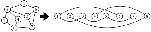
Figure 1: An example of a degeneracy ordering for a $2$-degenerate graph $G$. In this ordering, each vertex $v$ is adjacent to vertices at most two whose indices are larger than $v$.

The bottle-neck of EDS is the maintenance of candidate sets. Let $X$ be a dominating set and $Y$ be a child of $X$. We can easily see that the time complexity of EDS is $O\left(\Delta^{2}\right)$ time per solution since a removed vertex $u\in C\left(X\right)\setminus C\left(Y\right)$ has the distance at most two from $v$. In this section, we improve EDS by focusing on the degeneracy of an input graph $G$. $G$ is a $k$-degenerate graph [Lick:CJM:1970] if for any induced subgraph $H$ of $G$, the minimum degree in $H$ is less than or equal to $k$. The degeneracy of $G$ is the smallest $k$ such that $G$ is $k$-degenerate. A $k$-degenerate graph has a good vertex ordering. The definition of orderings of vertices in $G$, called a degeneracy ordering of $G$, is as follows: for any vertex $v$ in $G$, the number of vertices that are larger than $v$ and adjacent to $v$ is at most $k$. We show an example of a degeneracy ordering of a graph in Fig. 1. Matula and Beck show that the degeneracy and a degeneracy ordering of $G$ can be obtained in $O\left(n+m\right)$ time [Matula:Beck:JACM:1983]. Our proposed algorithm EDS-D, shown in Algorithm 2, achieves amortized $O\left(k\right)$ time enumeration by using this good ordering. In what follows, we fix some degeneracy ordering of $G$ and number the indices of vertices from $1$ to $n$ according to the degeneracy ordering. We assume that for each vertex $v$ and each dominating set $X$, $N[v]$ and $C\left(X\right)$ are stored in a doubly linked list and sorted by the ordering. Note that the larger neighbors of $v$ can be listed in $O\left(k\right)$ time. Let us denote by $V^{<v}=\left\{1,2,\dots,v-1\right\}$ and $V^{v<}=\left\{v+1,\dots n\right\}$. Moreover, $A^{<v}=A\cap V^{v<}$ and $A^{v<}=A\cap V^{<v}$ for a subset $A$ of $V$. We first show the relation between $C\left(X\right)$ and $C\left(Y\right)$.

Lemma 5.

Let $X$ be a dominating set of $G$ and $Y$ be a child of $X$. Then, $C\left(Y\right)\subset C\left(X\right)$.

Proof.

Let $Z$ be a child of $Y$. Hence, $pv\left(Z\right)\in X$ and $pv\left(Z\right)\in C\left(Y\right)$. From the definition of $pv\left(Z\right)$, $pv\left(Z\right)=\min{V\setminus Z}$. Moreover, since $V\setminus X\subset V\setminus Z$, $pv\left(Z\right)\leq\min{V\setminus X}$. Therefore, $pv\left(Z\right)\in C\left(X\right)$. ∎

From the Lemma 5, for any $v\in C\left(X\right)$, what we need to obtain the candidate set of $Y$ is to compute $Del\left(X,pv\left(Y\right)\right)=C\left(X\right)\setminus C\left(Y\right)$, where $Y=X\setminus\left\{v\right\}$. In addition, we can easily sort $C\left(Y\right)$ by the degeneracy ordering if $C\left(X\right)$ is sorted. In what follows, we denote by $Del_{1}\left(X,v\right)=\left\{u\in C\left(X\right)^{<v}\mathrel{}\middle|\mathrel{}N[u]\cap X=\left\{u,v\right\}\right\}$, $Del_{2}\left(X,v\right)=\left\{u\in C\left(X\right)^{<v}\mathrel{}\middle|\mathrel{}\exists w\in V\setminus(X\setminus\left\{v\right\})(N[w]\cap X=\left\{u,v\right\})\right\}$, and $Del_{3}\left(X,v\right)=C\left(X\right)^{v\leq}$. Next, we show the time complexity for obtaining $Del\left(X,pv\left(Y\right)\right)$.

Lemma 6.

For each $v\in C\left(X\right)$, $Del\left(X,v\right)=Del_{1}\left(X,v\right)\cup Del_{2}\left(X,v\right)\cup Del_{3}\left(X,v\right)$ holds.

Proof.

$Del\left(X,v\right)\supseteq Del_{1}\left(X,v\right)\cup Del_{2}\left(X,v\right)\cup Del_{3}\left(X,v\right)$ is trivial since $X\setminus\left\{u,v\right\}$ is not dominating set for each $u\in Del_{1}\left(X,v\right)\cup Del_{2}\left(X,v\right)$ and the parent of $X\setminus\left\{u,v\right\}$ is not $X\setminus\left\{v\right\}$ for each $u\in Del_{3}\left(X,v\right)$. We next prove $Del\left(X,v\right)\subseteq Del_{1}\left(X,v\right)\cup Del_{2}\left(X,v\right)\cup Del_{3}\left(X,v\right)$. Let $u$ be a vertex in $Del\left(X,v\right)$. Suppose that $X\setminus\left\{u,v\right\}$ is a dominating set. Since $\mathcal{P}\left(X\setminus\left\{u,v\right\}\right)\neq X\setminus\left\{v\right\}$, $v<u$. Thus, $u\in Del_{3}\left(X,v\right)$. Suppose that $X\setminus\left\{u,v\right\}$ is not a dominating set, that is, $N[X\setminus\left\{u,v\right\}]\neq V$. This implies that there exists a vertex $w$ in $V$ such that $w$ is not dominated by any vertex in $X\setminus\left\{u,v\right\}$. Note that $w$ may be equal to $u$ or $v$. Hence, $N[w]\cap X=\left\{u,v\right\}$ and the statement holds. ∎

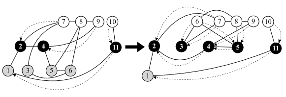
Figure 2: Let $X$ be a dominating set $\left\{1,2,3,4,5,6,11\right\}$. An example of the maintenance of $C\left(X\right)$ and $\mathcal{D}(X)$. Each dashed directed edge is stored in $\mathcal{D}(X)$, and each solid edge is an edge in $G$. A directed edge $(u,v)$ implies $v\in D_{u}(X)$. The index of each vertex is according to a degeneracy ordering. White, black, and gray vertices belong to $V\setminus X$, $X\setminus C\left(X\right)$, and $C\left(X\right)$, respectively. When EDS-D removes vertex $6$, $C\left(X\setminus\left\{6\right\}\right)=\left\{1\right\}$.

We show an example of dominated list and a maintenance of $C\left(X\right)$ in Fig. 2. To compute a candidate set efficiently, for each vertex $u$ in $V$, we maintain the vertex lists $D_{u}(X)$ for $X$. We call $D_{u}(X)$ the dominated list of $u$ for $X$. The definition of $D_{u}(X)$ is as follows: If $u\in V\setminus X$, then $D_{u}(X)=N(u)\cap(X\setminus C\left(X\right))$. If $u\in X$, then $D_{u}(X)=N(u)^{<u}\cap(X\setminus C\left(X\right))$. For brevity, we write $D_{u}$ as $D_{u}(X)$ if no confusion arises. We denote by $\mathcal{D}(X)=\bigcup_{u\in V}\left\{D_{u}\right\}$. By using $\mathcal{D}(X)$, we can efficiently find $Del_{1}\left(X,v\right)$ and $Del_{2}\left(X,v\right)$.

Lemma 7.

For each vertex $v\in C\left(X\right)$, we can compute $N(v)\cap C\left(X\right)$ and $N(v)^{v<}\cap X$ in $O\left(k\right)$ time on average over all children of $X$.

Proof.

Since $G$ is $k$-degenerate, $G[C\left(X\right)]$ is also $k$-degenerate. Thus, the number of edges in $G[C\left(X\right)]$ is at most $k\left|C\left(X\right)\right|$. Remind that $C\left(X\right)$ is sorted by the degeneracy ordering. Hence, by scanning vertices of $C\left(X\right)$ from the smallest vertex to the largest one, for each $v$ in $C\left(X\right)$, we can obtain $N(v)\cap C\left(X\right)$ in $O\left(k\right)$ time on average over all children of $X$. Since $N(v)^{v<}$ is the larger $v$’s neighbors set, the size is at most $k$. Hence, the statement holds. ∎

Lemma 8.

Let $X$ be a dominating set of $G$. Suppose that for each vertex $u$ in $G$, we can obtain the size of $D_{u}$ in constant time. Then, for each vertex $v\in C\left(X\right)$, we can compute $Del_{1}\left(X,v\right)$ in $O\left(k\right)$ time on average over all children of $X$.

Proof.

Since every vertex $u$ in $Del_{1}\left(X,v\right)$ is adjacent to $v$, $Del_{1}\left(X,v\right)\subseteq N(v)\cap C\left(X\right)$. To compute $Del_{1}\left(X,v\right)$, we need to check whether $N[u]\cap X=\left\{u,v\right\}$ or not. We first consider smaller neighbors of $u$. Before computing $Del_{1}\left(X,v\right)$ for every vertex $v$, we record the size of $D_{u}$ of $u\in C\left(X\right)$ in $O\left(\left|C\left(X\right)\right|\right)$ time. $D_{u}=\emptyset$ if and only if there are no smaller neighbors of $u$ in $X^{<u}\setminus C\left(X\right)$. Moreover, the number of edges in $G[C\left(X\right)]$ is at most $k\left|C\left(X\right)\right|$ from the definition of the degeneracy. Thus, this part can be done in $O\left(\sum_{v\in C\left(X\right)}\left|N(v)\cap C\left(X\right)\right|\right)$ total time and in $O\left(k\right)$ time per each vertex in $C\left(X\right)$. We next consider larger neighbors. Again, before computing $Del_{1}\left(X,v\right)$ for every vertex $v$, from Lemma 7 and the degeneracy of $G$, we can check all of the larger neighbors of $u\in C\left(X\right)$ in $O\left(k\left|C\left(X\right)\right|\right)$ time. Thus, as with the smaller case, the checking for the larger part also can be done in $O\left(k\right)$ time on average over all children of $X$. Hence, the statement holds. ∎

Lemma 9.

Suppose that for each vertex $w$ in $G$, we can obtain the size of $D_{w}$ in constant time. For each vertex $v\in C\left(X\right)$, we can compute $Del_{2}\left(X,v\right)$ in $O\left(k\right)$ time on average over all children of $X$.

Proof.

Let $u$ be a vertex in $Del_{2}\left(X,v\right)$. Then, there exists a vertex $w$ such that $N[w]\cap X=\left\{u,v\right\}$ and $w\in N[v]\cap(V\setminus(X\setminus\left\{v\right\})$. In addition, for any vertex $v^{\prime}$ in $C\left(X\right)$, $pv\left(X\setminus\left\{v^{\prime}\right\}\right)=v^{\prime}$. Thus, $v\leq w$ and $u<w$ hold. Before computing $Del_{2}\left(X,v\right)$ for every vertex $v$, by scanning all larger neighbors $w^{\prime}$ of vertices of $C\left(X\right)$, we can list such vertices $w^{\prime}$ such that $w^{\prime}>\max\left\{C\left(X\right)\right\}$, $\left|N[w^{\prime}]\cap C\left(X\right)\right|=2$, and $w^{\prime}\in V\setminus(X\setminus\left\{v\right\})$ in $O\left(k\left|C\left(X\right)\right|\right)$ time since $G$ is $k$-degenerate. If $D_{w^{\prime}}\neq\emptyset$, that is, $w^{\prime}$ has a neighbor in $X\setminus C\left(X\right)$, then $\left|N[w]\cap X\right|>2$. Thus, since we can check the size of $D_{w^{\prime}}$ in constant time, we can compute $Del_{2}\left(X,v\right)$ in $O\left(k\right)$ time on average over all children of $X$. ∎

In Lemma 8 and Lemma 9, we assume that the dominated lists were computed when we compute $Del\left(X,v\right)$ for each vertex $v$ in $C\left(X\right)$. We next consider how we maintain $\mathcal{D}$. Next lemmas show the transformation from $D_{u}(X)$ to $D_{u}(Y)$ for each vertex $u$ in $G$.

Lemma 10.

Let $X$ be a dominating set, $v$ be a vertex in $C\left(X\right)$, and $Y=X\setminus\left\{v\right\}$. For each vertex $u\in G$ such that $u\neq v$, $D_{u}(Y)=D_{u}(X)\cup(N(u)^{<u}\cap(Del_{1}\left(X,v\right)\cup Del_{2}\left(X,v\right)))\cup(N(u)^{<u}\cap(Del_{3}\left(X,v\right)\setminus\left\{v\right\}))$.

Proof.

Let $X_{\bar{C}}=X\setminus C\left(X\right)$. Suppose that $u\in Y$. From the definition, $D_{u}(X)=N(u)^{<u}\cap X_{\bar{C}}$. From the distributive property,

$$L = D_{u}(X)\cup(N(u)^{<u}\cap(Del_{1}\left(X,v\right)\cup Del_{2}\left(X,v\right)))\cup(N(u)^{<u}\cap(Del_{3}\left(X,v\right)\setminus\left\{v\right\}))$$

$$= N(u)^{<u}\cap(X_{\bar{C}}\cup(Del\left(X,v\right)\setminus\left\{v\right\}))$$

$$= N(u)^{<u}\cap(Y\setminus C\left(Y\right))$$

Since $X_{\bar{C}}\cup(Del\left(X,v\right)\setminus\left\{v\right\})=Y\setminus C\left(Y\right)$. Suppose that $u\in V\setminus X$. From the parent-child relation, $pv\left(Y\right)<u$ holds. Since $Del\left(X,v\right)\subseteq V^{<u}$, $N(u)^{<u}\cap(Del_{1}\left(X,v\right)\cup Del_{2}\left(X,v\right))=N(u)\cap(Del_{1}\left(X,v\right)\cup Del_{2}\left(X,v\right))$, and $N(u)^{<u}\cap(Del_{3}\left(X,v\right)\setminus\left\{v\right\})=N(u)\cap(Del_{3}\left(X,v\right)\setminus\left\{v\right\})$. From the definition, $D_{u}(X)=N(u)\cap X_{\bar{C}}$,

$$L = D_{u}(X)\cup(N(u)^{<u}\cap(Del_{1}\left(X,v\right)\cup Del_{2}\left(X,v\right)))\cup(N(u)^{<u}\cap(Del_{3}\left(X,v\right)\setminus\left\{v\right\}))$$

$$= (N(u)\cap X_{\bar{C}})\cup(N(u)\cap(Del_{1}\left(X,v\right)\cup Del_{2}\left(X,v\right)))\cup(N(u)\cap(Del_{3}\left(X,v\right)\setminus\left\{v\right\}))$$

$$= N(u)\cap(X_{\bar{C}}\cup(Del_{1}\left(X,v\right)\cup Del_{2}\left(X,v\right))\cup(Del_{3}\left(X,v\right)\setminus\left\{v\right\}))$$

$$= N(u)\cap(X_{\bar{C}}\cup(Del\left(X,v\right)\setminus\left\{v\right\}))$$

$$= N(u)\cap(Y\setminus C\left(Y\right))$$

Hence, the statement holds. ∎

Lemma 11.

Let $X$ be a dominating set, $v$ be a vertex in $C\left(X\right)$, and $Y=X\setminus\left\{v\right\}$. $D_{v}(Y)=D_{v}(X)\cup(N(v)^{<v}\cap(Del_{1}\left(X,v\right)\cup Del_{2}\left(X,v\right)))\cup(N(v)^{v<}\cap X)$.

Proof.

Since $Del_{1}\left(X,v\right)\cup Del_{2}\left(X,v\right)\subseteq V^{<v}$ and $Del_{3}\left(X,v\right)\cap V^{<v}=\emptyset$, $N(v)^{<v}\cap(Del_{1}\left(X,v\right)\cup Del_{2}\left(X,v\right))=N(v)^{<v}\cap Del\left(X,v\right)$. By the same discussion as Lemma 10, $L=D_{v}(X)\cup(N(v)^{<v}\cap Del\left(X,v\right))=N(v)^{<v}\cap(Y\setminus C\left(Y\right))$. Since $Y=X\setminus\left\{v\right\}$, $N(v)^{v<}\cap Y=N(v)^{v<}\cap X$. Moreover, since $X^{<v}=Y^{<v}$ and $C\left(Y\right)^{v<}=\emptyset$, $N(v)^{v<}\cap(Y\setminus C\left(Y\right))=N(v)^{v<}\cap X$. Since $L=(N(v)^{v<}\cup N(v)^{<v})\cap(Y\setminus C\left(Y\right))=D_{v}(Y)$, the statement holds. ∎

We next consider the time complexity for obtaining the dominated lists for children of $X$. From Lemma 10 and Lemma 11, a naïve method for the computation needs $O\left(k\left|Del\left(X,v\right)\right|+k\right)$ time for each vertex $v$ of $X$ since we can list all larger neighbors of any vertex in $O\left(k\right)$ time. However, if we already know $C\left(W\right)$ and $\mathcal{D}(W)$ for a child $W$ of $X$, then we can easily obtain $\mathcal{D}(Y)$, where $Y$ is the child of $X$ immediately after $W$. The next lemma plays a key role in EDS-D. Here, for any two sets $A,B$, we denote by $A\oplus B=(A\setminus B)\cup(B\setminus A)$.

Lemma 12.

Let $X$ be a dominating set, $v,u$ be vertices in $C\left(X\right)$ such that $u$ has the maximum index in $C\left(X\right)^{<v}$, $Y=X\setminus\left\{u\right\}$, and $W=X\setminus\left\{v\right\}$. Suppose that we already know $C\left(Y\right)\oplus C\left(W\right)$, $\mathcal{D}(W)$, $Del\left(X,v\right)$, and $Del\left(X,u\right)$. Then, we can compute $\mathcal{D}(Y)$ in $O\left(k\left|C\left(Y\right)\oplus C\left(W\right)\right|+k\right)$ time.

Proof.

Suppose that $z$ is a vertex in $G$ such that $z\neq v$ and $z\neq u$. From the definition, $D_{z}(W)\setminus D_{z}(Y)=(Del\left(X,v\right)\setminus Del\left(X,u\right))\cap N(z)^{<z}$ and $D_{z}(Y)\setminus D_{z}(W)=(Del\left(X,u\right)\setminus Del\left(X,v\right))\cap N(z)^{<z}$. Hence, we first compute $Del\left(X,v\right)\oplus Del\left(X,u\right)$. Now, $(C\left(X\right)\setminus C\left(W\right))\oplus(C\left(X\right)\setminus C\left(Y\right))=C\left(W\right)\oplus C\left(Y\right)$. Next, for each vertex $c$ in $C\left(W\right)\oplus C\left(Y\right)$, we check whether we add to or remove $c$ from $D_{z}(Y)$ or not. Note that added or removed vertices from $D_{z}(Y)$ is a smaller neighbor of $z$. From the definition, if $c\notin D_{z}(Y)$ or $c\in D_{z}(X)$, then we add $c$ to $D_{z}(Y)$. Otherwise, we remove $c$ from $D_{z}(Y)$. Thus, since each vertex in $C\left(W\right)\oplus C\left(Y\right)$ has at most $k$ larger neighbors, for all vertices other than $u$ and $v$, we can compute the all dominated lists in $O\left(k\left|C\left(W\right)\oplus C\left(Y\right)\right|\right)$ time. Next we consider the update for $D_{u}(Y)$ and $D_{v}(Y)$. Note that from the definition, $D_{v}(W)$ and $D_{u}(Y)$ contain larger neighbors of $v$ and $u$, respectively. However, the number of such neighbors is $O\left(k\right)$. Finally, since $v$ belongs to $Y$, $v\in D_{u^{\prime}}(Z)$ if $u^{\prime}\in N(v)^{v<}$ for any vertex $u^{\prime}$. Thus, as with the above discussion, we can compute $D_{u}(Y)$ and $D_{v}(Y)$ in $O\left(k\left|C\left(W\right)\oplus C\left(Y\right)\right|+k\right)$ time. ∎

Lemma 13.

Let $X$ be a dominating set. Then, AllChildren($X,C\left(X\right),\mathcal{D}(X)$) of EDS-D other than recursive calls can be done in $O\left(k\left|ch(X)\right|+k\left|gch(X)\right|\right)$ time.

Proof.

We first consider the time complexity of Cand-D. From Lemma 8 and Lemma 9, Cand-D correctly computes $Del_{1}\left(X,v\right)$ and $Del_{2}\left(X,v\right)$ in from line 2 to line 2 and from line 2 to line 2, respectively. For each loop from line 2, the algorithm picks the largest vertex in $C$. This can be done in $O\left(1\right)$ since $C$ is sorted. The algorithm needs to remove vertices in $Del_{3}\left(X,v\right)$. This can be done in line 2 and in $O\left(1\right)$ time since $v$ is the largest vertex. Thus, for each vertex $v$ in $C\left(X\right)$, $C\left(X\setminus\left\{v\right\}\right)$ can be obtained in $O\left(k\right)$ time on average. Hence, for all vertices in $C\left(X\right)$, the candidate sets can be computed in $O\left(k\left|ch(X)\right|\right)$ time. Next, we consider the time complexity of DomList. Before computing DomList, EDS-D already computed $C\left(Y\right)\oplus C\left(W\right)$, $\mathcal{D}(W)$, $Del\left(X,v\right)$, and $Del\left(X,v^{\prime}\right)$. Note that we can compute $C\left(Y\right)\oplus C\left(W\right)$ when we compute $C\left(Y\right)$ and $C\left(W\right)$. Here, $W$ is the previous dominating set, $C^{\prime}$ stores $C\left(W\right)$, and $\mathcal{D}^{\prime}$ stores $\mathcal{D}(W)$. Thus, by using Lemma 12, we can compute $\mathcal{D}(Y)$ in $O\left(k\left|C\left(Y\right)\oplus C\left(W\right)\right|+k\right)$ time. In addition, for all vertices in $C\left(X\right)$, the dominated lists can be computed in $O\left(k\left|C\left(X\right)\right|+k\left|gch(X)\right|\right)$ time since $Y$ has at least $\left|C\left(W\right)\setminus C\left(Y\right)\right|-1$ children and $\left|gch(X)\right|$ is at least the sum of $\left|C\left(W\right)\setminus C\left(Y\right)\right|-1$ over all $Y\in\left\{X\setminus\left\{v\right\}\mathrel{}\middle|\mathrel{}v\in C\left(X\right)\right\}$ and the previous solution $W$ of $Y$. When EDS-D copies data such as $\mathcal{D}$, EDS-D only copies the pointer of these data. By recording operations of each line, EDS-D restores these data when backtracking happens. These restoring can be done in the same time of the above update computation. ∎

Theorem 14.

EDS-D enumerates all dominating sets in $O\left(k\right)$ time per solution in a $k$-degenerate graph by using $O\left(n+m\right)$ space.

Proof.

The parent-child relation of EDS-D and EDS are same. From Lemma 5 and Lemma 6, EDS-D correctly computes all children. Hence, the correctness of EDS-D is shown by the same manner of Theorem 4. We next consider the space complexity of EDS-D. For any vertex $v$ in $G$, if $v$ is removed from a data structure used in EDS-D on a recursive procedure, $v$ will never be added to the data structure on descendant recursive procedures. In addition, for each recursive procedure, the number of data structures that are used in the procedure is constant. Hence, the space complexity of EDS-D is $O\left(n+m\right)$. We finally consider the time complexity. Each recursive procedure needs $O\left(k\left|ch(X)\right|+k\left|gch(X)\right|\right)$ time from Lemma 13. Thus, the time complexity of EDS-D is $O\left(k\sum_{X\in\mathcal{S}}(\left|ch(X)\right|+\left|gch(X)\right|)\right)$, where $\mathcal{S}$ is the set of solutions. Now, $O\left(\sum_{X\in\mathcal{S}}(\left|ch(X)\right|+\left|gch(X)\right|)\right)=O\left(\left|\mathcal{S}\right|\right)$. Hence, the statement holds. ∎

4 Efficient Enumeration for Graphs with Girth at Least Nine

1 Procedure EDS-G($G=(V,E)$) // $G$: an input graph

2       for $v\in V$ do  $f_{v}\leftarrow\mathtt{False}$ ;

3       AllChildren $(V,V,\left\{f_{1},\dots,f_{\left|V\right|}\right\},G)$;

4      

5Procedure AllChildren $(X,C,F,G)$

6       Output $X$;

7       for $v\in C\left(X\right)$ do // $v$ is the largest vertex in $C$

8             $Y\leftarrow X\setminus\left\{v\right\}$;

9             $(C\left(Y\right),F(Y),G(Y))\leftarrow$ Cand-G $(v,C,F,G)$;

10             AllChildren $(Y,C\left(Y\right),F(Y),G(Y))$;

11             for $u\in N_{G}(v)$ do

12                   if $u\in C$ then  $f_{u}\leftarrow\mathtt{True}$ ;

13                  else  $G\leftarrow G\setminus\left\{u\right\}$ ;

14                  

15            $G\leftarrow G\setminus\left\{v\right\}$;

             $C\leftarrow C\setminus\left\{v\right\}$;

              // Remove vertices in $Del_{3}\left(X,v\right)$.

16            

17Procedure Cand-G $(v,C,F,G)$

18       $Del_{1}\leftarrow\emptyset$; $Del_{2}\leftarrow\emptyset$;

19       for $u\in N_{G}(v)$ do

20             if $N_{G}[u]\cap X=\left\{u,v\right\}$ and $f_{u}=\mathtt{False}$ then  $Del_{1}\leftarrow Del_{1}\cup\left\{u\right\}$ ;

21            else if $\exists w(N_{G}[u]\cap X=\left\{w,v\right\})$ then  $Del_{2}\leftarrow Del_{2}\cup\left\{w\right\}$ ;

22            

23       $C^{\prime}\leftarrow C\setminus(Del_{1}\cup Del_{2}\cup\left\{v\right\})$;

24       for $u\in N^{\prime}[Del_{1}\cup Del_{2}]$ do // Lemma 18

25             $f_{u}\leftarrow\mathtt{True}$;

26             if $u\notin C^{\prime}$ then  $G\leftarrow G\setminus\left\{u\right\}$ ;

27            

28      if $f_{v}=\mathtt{True}$ then $G\leftarrow G\setminus\left\{v\right\}$;

29       return $(C^{\prime},F,G)$;

30      

Algorithm 3 EDS-G enumerates all dominating sets in $O\left(1\right)$ time per solution for a graph with girth at least nine.

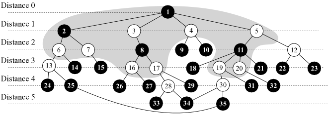
Figure 3: An example of $G_{v}(X)$, where $v=1$. The vertices in the grey area are $Del^{\prime}\left(X,v\right)\cup(G_{v}(X)\setminus G(Y))\cup(N^{\prime}_{v}(v)\setminus X)$. Each horizontal line represents the distance between $1$ and any vertex.

In this section, we propose an optimum enumeration algorithm EDS-G for graphs with girth at least nine, where the girth of a graph is the length of a shortest cycle in the graph. That is, the proposed algorithm runs in constant amortized time per solution for such graphs. The algorithm is shown in Algorithm 3. To achieve constant amortized time enumeration, we focus on the local structure $G_{v}(X)$ for $(X,v)$ of $G$ defined as follows: $G_{v}(X)=G[(V\setminus N[X\setminus C\left(X\right)^{\leq v}])\cup C\left(X\right)^{\leq v}]$. Fig. 3 shows an example of $G_{v}(X)$. $G_{v}(X)$ is a subgraph of $G$ induced by vertices that (1) are dominated by vertices only in $C\left(X\right)^{\leq v}$ or (2) are in $C\left(X\right)^{\leq v}$. Intuitively speaking, we can efficiently enumerate solutions by using the local structure and ignoring vertices in $G\setminus G_{v}(X)$ since the number of solutions that are generated according to the structure is enough to reduce the amortized time complexity to constant. We denote by $G(X)=G[(V\setminus N[X\setminus C\left(X\right)])\cup C\left(X\right)]$ the local structure for $(X,v_{*})$ of $G$, where $v_{*}$ is the largest vertex in $G$.

We first consider the correctness of EDS-G. The parent-child relation between solutions used in EDS-G is the same as in EDS. Suppose that $X$ and $Y$ are dominating sets such that $X$ is the parent of $Y$. Recall that, from Lemma 6, $C\left(X\right)\setminus C\left(Y\right)=Del\left(X,v\right)$, where $X=Y\cup\left\{v\right\}$. We denote by $f_{v}(u,X)=\mathtt{True}$ if there exists a neighbor $w$ of $u$ such that $w\in X\setminus C\left(X\right)^{\leq v}$; Otherwise $f_{v}(u,X)=\mathtt{False}$. Thus, Cand-G correctly computes $Del_{1}\left(X,v\right)$ and $Del_{2}\left(X,v\right)$ from line 3 to 3. Moreover, in line 3, vertices in $Del_{3}\left(X,v\right)$ are removed from $C\left(X\right)$ and hence, Cand-G also correctly computes $C\left(X\setminus\left\{v\right\}\right)$. Moreover, for each vertex $w$ removed from $G$ during enumeration, $w$ is dominated by some vertices in $G$. Hence, by the same discussion as Theorem 4, we can show that EDS-G enumerates all dominating sets. In the remaining of this section, we show the time complexity of EDS-G. Note that $G_{v}(X)$ does not include any vertex in $N[Del_{3}\left(X,v\right)\setminus\left\{v\right\}]\setminus C\left(X\right)^{\leq v}$. Hence, we will consider only vertices in $Del_{1}\left(X,v\right)\cup Del_{2}\left(X,v\right)\cup\left\{v\right\}$. We denote by $Del^{\prime}\left(X,v\right)=Del_{1}\left(X,v\right)\cup Del_{2}\left(X,v\right)\cup\left\{v\right\}$. We first show the time complexity for updating the candidate sets.

In what follows, if $v$ is the largest vertex in $C\left(X\right)$, then we simply write $f(u,X)$ as $f_{v}(u,X)$. We denote by $N^{\prime}_{v}(u)=N_{G_{v}(X)}(u)$, $N^{\prime}_{v}[u]=N^{\prime}_{v}(u)\cup\left\{u\right\}$, and $d^{\prime}_{v}(u)=\left|N^{\prime}_{v}(u)\right|$ if no confusion arises. Suppose that $G$ and $G_{v}(X)$ are stored in an adjacency list, and neighbors of a vertex are stored in a doubly linked list and sorted in the ordering.

Lemma 15.

Let $X$ be a dominating set, $v$ be a vertex in $C\left(X\right)$, and $u$ be a vertex in $G$. Then, $u\in Del_{1}\left(X,v\right)$ if and only if $N^{\prime}_{v}[u]\cap X=\left\{u,v\right\}$ and $f_{v}(u,X)=\mathtt{False}$.

Proof.

The only if part is obvious since $u,v\in C\left(X\right)^{\leq v}$ and $N[u]\cap X=\left\{u,v\right\}$. We next prove the if part. Since $f_{v}(u,x)=\mathtt{False}$, $N[u]\cap(X\setminus C\left(X\right)^{\leq v})=\emptyset$. Moreover, since $(N^{\prime}_{v}[u]\cap X)\subseteq C\left(X\right)^{\leq v}$, $N[u]\cap X=N^{\prime}_{v}[u]\cup(N[u]\cap(X\setminus C\left(X\right)^{v<}))=\left\{u,v\right\}$. Hence, the statement holds. ∎

Lemma 16.

Let $X$ be a dominating set, $v$ be a vertex in $C\left(X\right)$, and $u$ be a vertex in $G$. Then, $u\in Del_{2}\left(X,v\right)$ if and only if there is a vertex $w$ in $G_{v}(X)$ such that $N^{\prime}_{v}[w]\cap X=\left\{u,v\right\}$.

Proof.

The only if part is obvious since $u,v\in C\left(X\right)^{\leq v}$ and there is a vertex $w$ such that $N[w]\cap X=\left\{u,v\right\}$. We next show the if part. Since $w\in G_{v}(X)$, $w\in C\left(X\right)^{\leq v}$ or $w\notin X\cup N[X\setminus C\left(X\right)^{\leq v}]$. Moreover, since $N^{\prime}[w]=\left\{u,v\right\}$, $w\notin X$, that is, $w\notin C\left(X\right)$. Hence, $w\notin N[X\setminus C\left(X\right)^{\leq v}]$. Therefore, $N[w]\cap X=(N^{\prime}_{v}[w]\cap X)\cup(N[w]\cap(X\setminus C\left(X\right)^{v<}))=\left\{u,v\right\}$ and the statement holds. ∎

Lemma 17.

Let $X$ be a dominating set and $v$ be a vertex in $C\left(X\right)$. Suppose that for any vertex $u$, we can check the number of $u$’s neighbors in the local structure $G_{v}(X)$ and the value of $f_{v}(u,X)$ in constant time. Then, we can compute $C\left(X\setminus\left\{v\right\}\right)$ from $C\left(X\right)^{\leq v}$ in $O\left(d^{\prime}_{v}(v)\right)$ time

Proof.

Since $Del_{3}\left(X,v\right)\cap C\left(X\setminus\left\{v\right\}\right)=\emptyset$, $C\left(X\setminus\left\{v\right\}\right)\subseteq C\left(X\right)^{\leq v}$. Thus, we do not need to remove vertices in $Del_{3}\left(X,v\right)$ from $C\left(X\right)^{\leq v}$. From Lemma 15, for each vertex $u\in N^{\prime}_{v}(v)$, we can check whether $u\in Del_{1}\left(X,v\right)$ or not in constant time by confirming that $f_{v}(u,X)=\mathtt{False}$ and $\left|N^{\prime}_{v}(u)\right|=2$. Moreover, from Lemma 16, for each vertex $w\in N^{\prime}_{v}(v)$, we can compute $Del_{2}\left(X,v\right)$ by listing vertices in $u\in C\left(X\right)^{\leq v}$ such that $N^{\prime}[w]\cap X=\left\{u,v\right\}$ or not. Note that since any vertex in $X^{<v}$ belongs to $X$, $N^{\prime}[w]\cap X=\left\{u,v\right\}$ if $f_{v}(w,X)=\mathtt{False}$, $\left|N^{\prime}[w]\right|=2$, and $u$ and $v$ are adjacent to $w$. Hence, the statement holds. ∎

Lemma 18.

Let $X$ be a dominating set, $v$ be a vertex in $C\left(X\right)$, and $Y=X\setminus\left\{v\right\}$. Then, we can compute $G(Y)$ from $G_{v}(X)$ in $O\left(\sum_{u\in Del^{\prime}\left(X,v\right)}d^{\prime}_{v}(u)+\sum_{u\in G_{v}(X)\setminus G(Y)}d^{\prime}_{v}(u)\right)$ time. Note that $N^{\prime}_{v}(u)=N_{G_{v}(X)}(u)$ and $d^{\prime}_{v}(u)=\left|N^{\prime}_{v}(u)\right|$.

Proof.

From the definition, $V(G(Y))\subseteq V(G_{v}(X))$. Let us denote by $u$ a vertex in $G_{v}(X)$ but not in $G(Y)$ such that $u\neq v$. This implies that (A) $u$ is dominated by some vertex in $Y\setminus C\left(Y\right)$ and (B) $u\notin C\left(Y\right)$. Thus, for any vertex $u^{\prime}\notin N^{\prime}_{v}[Del^{\prime}\left(X,v\right)\setminus\left\{v\right\}]$, $u^{\prime}\in G_{v}(X)$ if and only if $u^{\prime}\in G(Y)$. Hence, we can find such vertex $u$ by checking whether for each vertex $w\in N^{\prime}_{v}[Del^{\prime}\left(X,v\right)]$, $w$ satisfies (A) and (B). Before checking, we first update the value of $f$. This can be done by checking all the vertices in $N^{\prime}_{v}[Del^{\prime}\left(X,v\right)]$ and in $O\left(1\right)$ time per vertex. Hence, this update needs $O\left(\sum_{w\in Del^{\prime}\left(X,v\right)}d^{\prime}_{v}(w)\right)$ time. If $w$ satisfies these conditions, that is, $f_{v}(w,X)=\mathtt{False}$, $f(w,Y)=\mathtt{True}$, and (B), then we remove $w$ and edges that are incident to $w$ from $G_{v}(X)$. This needs $O\left(\sum_{w\in G_{v}(X)\setminus G(Y)}d^{\prime}_{v}(w)\right)$ total time for removing vertices. Thus, the statement holds. ∎

From Lemma 17 and Lemma 18, we can compute the local structure and the candidate set of $Y$ from those of $X$ in $O\left(\sum_{u\in Del^{\prime}\left(X,v\right)}d^{\prime}_{v}(u)+\sum_{u\in G_{v}(X)\setminus G(Y)}d^{\prime}_{v}(u)\right)$ time. We next consider the time complexity of the loop in line 3. In this loop procedure, EDS-G deletes all the neighbors $u$ of $v$ from $G_{v}(X)$ if $u\notin C\left(X\right)^{\leq v}$ because for each descendant $W$ of dominating set $Y^{\prime}$, $v\in W\setminus C\left(W\right)$, where $Y^{\prime}$ is a child of $X$ and is generated after $Y$. Thus, this needs $O\left(d^{\prime}_{v}(v)+\sum_{u\in N^{\prime}(v)\setminus X}d^{\prime}_{v}(u)\right)$ time. Hence, from the above discussion, we can obtain the following lemma:

Lemma 19.

Let $X$ be a dominating set, $v$ be a vertex in $C\left(X\right)$, and $Y=X\setminus\left\{v\right\}$. Then, AllChildren other than a recursive call runs in the following time bound:

$$O\left(\sum_{u\in Del^{\prime}\left(X,v\right)}d^{\prime}_{v}(u)+\sum_{u\in G_{v}(X)\setminus G(Y)}d^{\prime}_{v}(u)+\sum_{u\in N^{\prime}_{v}(v)\setminus X}d^{\prime}_{v}(u)\right).$$ (1)

Before we analyze the number of descendants of $X$, we show the following lemmas.

Lemma 20.

Let us denote by $Pen_{v}(X)=\left\{u\in Del^{\prime}\left(X,v\right)\mathrel{}\middle|\mathrel{}d^{\prime}_{v}(u)=1\right\}$. Then, $\sum_{v\in C\left(X\right)}\left|Pen_{v}(X)\right|$ is at most $\left|C\left(X\right)\right|$.

Proof.

Let $u$ be the largest vertex in $C\left(X\right)^{<v}$ and $w$ be a vertex in $G_{v}(X)\cap Del^{\prime}\left(X,v\right)$. If $w\in Del_{1}\left(X,v\right)$, then $d^{\prime}_{u}(w)=0$ since $w\in N^{\prime}_{v}(v)$. Otherwise, $w\in Del_{2}\left(X,v\right)$, then $d^{\prime}_{u}(w)=0$ since a vertex $x$ such that $N^{\prime}_{v}[x]=\left\{w,v\right\}$ is removed from $G_{v}(X)$. Hence, $Pen_{v}(X)\cap Pen_{u}(X)=\emptyset$. Moreover, for each $v\in C\left(X\right)$, $Pen_{v}(X)$ is a subset of $C\left(X\right)$. Hence, the union of $Pen_{v}(X)$ is a subset of $C\left(X\right)$ for each $v\in C\left(X\right)$. ∎

Let $v$ be a vertex in $C\left(X\right)$ and a pendant in $G_{v}(X)$. Since the number of such pendants is at most $\left|C\left(X\right)\right|$, the sum of degree of such pendants is at most $\left|C\left(X\right)\right|$ in each execution of AllChildren without recursive calls. Hence, the cost of deleting such pendants is $O\left(\left|C\left(X\right)\right|\right)$ time. Next, we consider the number of descendants of $X$. From Lemma 20, we can ignore such pendant vertices. Hence, for each $u\in Del^{\prime}\left(X,v\right)$, we will assume that $d^{\prime}_{v}(u)\geq 2$ below.

Lemma 21.

Let $X$ be a dominating set, $v$ be a vertex in $C\left(X\right)$, and $u$ be a vertex in $G_{v}(X)$. Then, $\left|N^{\prime}_{v}[u]\cap C\left(X\right)^{\leq v}\right|\geq 2$ if $u\notin C\left(X\right)$. Otherwise, $\left|N^{\prime}_{v}[u]\cap C\left(X\right)^{\leq v}\right|\geq 1$.

Proof.

If $u\in C\left(X\right)$, then $u\in N^{\prime}[u]\cap C\left(X\right)$. We assume that $u\notin C\left(X\right)$. Thus, $N^{\prime}[u]\cap(X\setminus C\left(X\right))=\emptyset$ from the definition of $G(X)$. If $\left|N^{\prime}[u]\cap C\left(X\right)\right|=0$, then $u$ is not dominated by any vertex. This contradicts $X$ is dominating set. If $\left|N^{\prime}[u]\cap C\left(X\right)\right|=1$, then $u$ is dominated only by the neighbor $w$ of $u$ in $C\left(X\right)$. This contradicts $w\in C\left(X\right)$. Hence, $\left|N[v]\cap C\left(X\right)\right|\geq 2$ if $v\notin C\left(X\right)$. ∎

Lemma 22.

Let $X$ be a dominating set, $v$ be a vertex in $C\left(X\right)$, and $Y$ be a dominating set $X\setminus\left\{v\right\}$. Then, $\left|C\left(Y\right)\right|$ is at least $\left|(N^{\prime}_{v}(v)\cap X)\setminus Del^{\prime}\left(X,v\right)\right|$.

Proof.

Let $u$ be a vertex in $(N^{\prime}_{v}(v)\cap X)\setminus Del^{\prime}\left(X,v\right)$. If $u\in C\left(X\right)$, then $u$ is also a candidate vertex in $C\left(Y\right)$ since $u\notin Del^{\prime}\left(X,v\right)$. Suppose that $u\notin C\left(X\right)$. Since $u\in G_{v}(X)$, $u$ is dominated by only candidate vertices of $X$. However, since $u\in X$, $u$ dominates it self and thus, this contradicts. Hence, the statement holds. ∎

Lemma 23.

Let $X$ be a dominating set, $v$ be a vertex in $C\left(X\right)$, and $Y$ be a dominating set $X\setminus\left\{v\right\}$. Then, $\left|C\left(Y\right)\right|$ is at least $\sum_{u\in N^{\prime}_{v}(v)\setminus X}(d^{\prime}_{v}(u)-1)$.

Proof.

Let $u$ be a vertex in $N^{\prime}_{v}(v)\setminus X$. That is, $u\notin C\left(X\right)$ and $N^{\prime}_{v}(u)\subseteq C\left(X\right)$. Thus, from Lemma 21, there is a vertex $w\in N^{\prime}_{v}(u)$ such that $w<v$. We consider the following two cases: (A) If $N^{\prime}_{v}(u)=\left\{v,w\right\}$, then $w\in Del^{\prime}\left(X,v\right)$. From the assumption, $w$ has at least one neighbor $x$ such that $x\neq u$. If $x\notin C\left(X\right)$, then there is a neighbor $y\in C\left(X\right)$ such that $y\neq w$. Suppose that $y\in Del^{\prime}\left(X,v\right)$. This implies that there is a cycle with length at most six. This contradicts the girth of $G$. Hence, $y\notin Del^{\prime}\left(X,v\right)$ and $Y\setminus\left\{y\right\}$ is a dominating set. If $x\in C\left(X\right)$, then $x\notin Del^{\prime}\left(X,v\right)$ from the definition of $Del^{\prime}\left(X,v\right)$ and the girth of $G$. Hence, $Y\setminus\left\{x\right\}$ is a dominating set. (B) Suppose $N^{\prime}_{v}(u)$ has a vertex $z\in C\left(X\right)$ such that $z\neq v$ and $z\neq w$. If both $z$ and $w$ are in $Del^{\prime}\left(X,v\right)$, then from the definition of $Del^{\prime}\left(X,v\right)$ and the girth of $G$, $G$ has a cycle with length at most five. Thus, without loss of generality, we can assume that $z\notin Del^{\prime}\left(X,v\right)$. This allows us to generate a child $Y\setminus\left\{z\right\}$ of $Y$. Since the girth of $G$ is at least nine, all children of $Y$ generated above are mutually distinct. Hence, the statement holds. ∎

Lemma 24.

Let $X$ be a dominating set, $v$ be a vertex in $C\left(X\right)$, and $Y$ be a dominating set $X\setminus\left\{v\right\}$. Then, $\left|C\left(Y\right)\right|$ is at least $\sum_{u\in Del^{\prime}\left(X,v\right)\setminus\left\{v\right\}}\left(d^{\prime}_{v}(u)-1\right)$.

Proof.

Let $u$ be a vertex in $Del^{\prime}\left(X,v\right)\setminus\left\{v\right\}$. From the assumption, there is a neighbor $w$ of $u$ in $G(X)$. We consider the following two cases: (A) Suppose that $w$ is in $G(Y)$. Since $u$ is in $Y\setminus C\left(Y\right)$, $w\in C\left(Y\right)$. Hence, $Y\setminus\left\{w\right\}$ is a child of $Y$. Suppose that for any two distinct vertices $x,y$ in $Del^{\prime}\left(X,v\right)\setminus\left\{v\right\}$, they have a common neighbor $w^{\prime}$ in $G(Y)$. If both $x$ and $y$ are in $Del_{2}\left(X,v\right)$, then there exist two vertex $z_{x},z_{y}$ such that $N^{\prime}_{v}[z_{x}]\cap X=\left\{x,v\right\}$ and $N^{\prime}_{v}[z_{y}]\cap X=\left\{y,v\right\}$, respectively. Therefore, there is a cycle $(v,z_{x},x,w^{\prime},y,z_{y},v)$ with length six. As with the above, if $x$ or $y$ in $Del_{1}\left(X,v\right)$, then there exists a cycle with length less than six since $\left\{x,v\right\}\in G$ or $\left\{x,v\right\}\in G$. This contradicts of the assumption of the girth of $G$. Hence, any pair vertices in $Del^{\prime}\left(X,v\right)$ has no common neighbors. Thus, in this case, all grandchildren of $X$ are mutually distinct. (B) Suppose that $w$ is not in $G(Y)$. Thus, if $w\in C\left(X\right)$, then $w\in Del^{\prime}\left(X,v\right)$. This implies that there is a cycle including $w$ and $u$ whose length is less than six. Hence, $w$ is not in $C\left(X\right)$. Then, from Lemma 21, there is a vertex $z$ in $N^{\prime}_{v}(w)\cap C\left(X\right)$ such that $z\neq u$. Since $u\in Del^{\prime}\left(X,v\right)\setminus\left\{v\right\}$, there is an edge between $u$ and $v$, or there is a vertex $c$ such that $\left\{u,c\right\}$ and $\left\{v,c\right\}$ are in $G_{v}(X)$. Again, if $z$ is in $Del^{\prime}\left(X,v\right)$, then there is a cycle with length less than seven. Thus, $z$ still belongs to $C\left(Y\right)$ and $X\setminus\left\{v,z\right\}$ is a dominating set. Next, we consider the uniqueness of $X\setminus\left\{v,z\right\}$. If there is a vertex $w^{\prime}$ such that $w^{\prime}\in N^{\prime}_{v}(u)$, $w^{\prime}\neq w$, $w$ and $w^{\prime}$ share a common neighbor $u^{\prime}$ other than $u$, then $(u,w,u^{\prime},w^{\prime})$ is a cycle. Hence, any pair neighbors of $u$ has no common neighbors. As with the above, any two distinct vertices in $Del^{\prime}\left(X,v\right)\setminus\left\{v\right\}$ also has no common vertex like $z$. If there are two distinct vertex $u,u^{\prime}\in Del^{\prime}\left(X,v\right)$ such that $u$ and $u^{\prime}$ has a common vertex like $z$, then there is a cycle with length at most eight even if $u,u^{\prime}\in Del_{2}\left(X,v\right)$. This contradicts the assumption of the girth, and thus, the statement holds. ∎

Lemma 25.

Let $X$ be a dominating set $v$ be a vertex in $C\left(X\right)$, and $Y$ be a dominating set $X\setminus\left\{v\right\}$. Then, the number of children and grandchildren of $Y$ is at least $\sum_{u\in G_{v}(X)\setminus\left(G(Y)\cup Del^{\prime}\left(X,v\right)\cup N^{\prime}_{v}(v)\right)}\left(d^{\prime}_{v}(u)-1\right)$.

Proof.

Let $u$ be a vertex in $G_{v}(X)\setminus(G(Y)\cup Del^{\prime}\left(X,v\right)\cup N^{\prime}_{v}(v))$. Since $u\notin Del^{\prime}\left(X,v\right)$ and $u\in G_{v}(X)\setminus G(Y)$, $u$ is not in $X$. Since $\left|N^{\prime}_{v}(u)\cap C\left(X\right)^{\leq v}\right|$ is greater than or equal to two from Lemma 21, there are two distinct vertices $w,w^{\prime}$ in $N^{\prime}_{v}(u)$. We assume that $w,w^{\prime}\in Del^{\prime}\left(X,v\right)$. From Lemma 6, the distance between $w$ and $v$ is at most two. Similarly, the distance between $w^{\prime}$ and $v$ is at most two. Hence, there is a cycle with the length at most six since $w\neq v$ and $w^{\prime}\neq v$. Thus, without loss of generality, we can assume that $w\notin Del^{\prime}\left(X,v\right)$. (A) Suppose that $\left|N^{\prime}_{v}(u)\right|=2$. If there is a vertex $u^{\prime}\in G_{v}(X)\setminus(G(Y)\cup Del^{\prime}\left(X,v\right)\cup N^{\prime}_{v}(v))$ such that $u^{\prime}\neq u$ and $w\in N^{\prime}(u)$, then as with Lemma 23, there is a short cycle. Hence, for each vertex such as $u$, there is a corresponding dominating set $X\setminus\left\{v,w\right\}$. (B) Suppose that there is a neighbor $w^{\prime\prime}\in N^{\prime}_{v}(u)\cap C\left(X\right)$. Then, as mentioned in above, there is a dominating set $X\setminus\left\{v,w,w^{\prime\prime}\right\}$. In addition, by the same discussion as Lemma 24, such generated dominating sets are mutually distinct. (C) Suppose that there is a neighbor $w^{\prime\prime}\in N^{\prime}_{v}(u)\setminus C\left(X\right)$. From Lemma 21, there are two vertices $z,z^{\prime}\in N^{\prime}(w^{\prime\prime})\cap C\left(X\right)$. Then, $z\notin Del^{\prime}\left(X,v\right)$ or $z^{\prime}\notin Del^{\prime}\left(X,v\right)$, and thus, we can assume that $z\notin Del^{\prime}\left(X,v\right)$. Therefore, there is a dominating set $X\setminus\left\{v,w,z\right\}$. Next, we consider the uniqueness of grandchildren of $Y$. Moreover, if there is a vertex $u^{\prime}$ such that $w,y\in N^{\prime}(u^{\prime})$ holds, such that $z\in N^{\prime}(y)$. Then, there is a cycle $(u,w,u^{\prime},y,z,w^{\prime\prime})$ with the length six. Hence, grandchildren of $Y$ are mutually distinct for each $u\in G(X)\setminus G(Y)\setminus Del^{\prime}\left(X,v\right)$. Thus, from (A), (B), and (C), the statement holds. ∎

Note that for any pair of candidate vertices $v$ and $v^{\prime}$, $X\setminus\left\{v\right\}$ and $X\setminus\left\{v^{\prime}\right\}$ do not share their descendants. Thus, from Lemma 22, Lemma 23, Lemma 24, and Lemma 25, we can obtain the following lemma:

Lemma 26.

Let $X$ be a dominating set. Then, the sum of the number of $X$’s children, grandchildren, and great-grandchildren is bounded by the following order:

$$\Omega\left(\left|C\left(X\right)\right|+\sum_{v\in C\left(X\right)}\left(\sum_{u\in Del^{\prime}\left(X,v\right)}d^{\prime}_{v}(u)+\sum_{u\in G_{v}(X)\setminus G(Y)}d^{\prime}_{v}(u)+\sum_{u\in N^{\prime}_{v}(v)\setminus X}d^{\prime}_{v}(u)\right)\right).$$ (2)

From Lemma 19, Lemma 20, and Lemma 26, each iteration outputs a solution in constant amortized time. Hence, by the same discussion of Theorem 14, we can obtain the following theorem.

Theorem 27.

For an input graph with girth at least nine, EDS-G enumerates all dominating sets in $O\left(1\right)$ time per solution by using $O\left(n+m\right)$ space.

Proof.

The correctness of EDS-G is shown by Theorem 4, Lemma 15, and Lemma 16. By the same discussion with Theorem 14, the space complexity of EDS-G is $O\left(n+m\right)$. We next consider the time complexity of EDS-G. From Lemma 19, Lemma 20, and Lemma 26. we can amortize the cost of each recursion by distributing $O\left(1\right)$ time cost to the corresponding descendant discussed in the above lemmas. Thus, the amortized time complexity of each recursion becomes $O\left(1\right)$. Moreover, each recursion outputs a solution. Hence, EDS-G enumerates all solutions in $O\left(1\right)$ amortized time per solution. ∎

5 Conclusion

In this paper, we proposed two enumeration algorithms. EDS-D solves the dominating set enumeration problem in $O\left(k\right)$ time per solution by using $O\left(n+m\right)$ space, where $k$ is a degeneracy of an input graph $G$. Moreover, EDS-G solves this problem in constant time per solution if an input graph has girth at least nine.

Our future work includes to develop efficient dominating set enumeration algorithms for dense graphs. If a graph is dense, then $k$ is large and $G$ has many dominating sets. For example, in the case of complete graphs, $k$ is equal to $n-1$ and every nonempty subset of $V$ is a dominating set. That is, the number of solutions for a dense graph is much larger than that for a sparse graph. This allows us to spend more time in each recursive call. However, EDS-D is not efficient for dense graphs although the number of solutions is large. Moreover, if $G$ is small girth, that is, $G$ is dense then EDS-G does not achieve constant amortized time enumeration. Hence, the dominating set enumeration problem for dense graphs is interesting.

References

- [1] D. Avis and K. Fukuda. Reverse search for enumeration. Discrete Appl. Math., 65(1):21–46, 1996.
- [2] E. Birmelé, R. A. Ferreira, R. Grossi, A. Marino, N. Pisanti, R. Rizzi, and G. Sacomoto. Optimal Listing of Cycles and st-Paths in Undirected Graphs. In Proc. SODA 2013 ACM, pages 1884–1896, 2013.
- [3] E. Boros, K. Elbassioni, V. Gurvich, and L. Khachiyan. Generating maximal independent sets for hypergraphs with bounded edge-intersections. In Proc. LATIN 2004, pages 488–498. Springer, 2004.
- [4] B. Brešar, M. A. Henning, and D. F. Rall. RAINBOW DOMINATION IN GRAPHS. Taiwanese J. Math., 12(1):213–225, 2008.
- [5] L. S. Chandran and C. Subramanian. Girth and treewidth. J. Combin. Theory Ser. B, 93(1):23–32, 2005.
- [6] S. Cohen, B. Kimelfeld, and Y. Sagiv. Generating all maximal induced subgraphs for hereditary and connected-hereditary graph properties. J. Comput. Syst. Sci., 74(7):1147 – 1159, 2008.
- [7] A. Conte, R. Grossi, A. Marino, and L. Versari. Sublinear-Space Bounded-Delay Enumeration for Massive Network Analytics: Maximal Cliques. In Proc. ICALP 2016, volume 55 of LIPIcs, pages 148:1–148:15. Schloss Dagstuhl–Leibniz-Zentrum fuer Informatik, 2016.
- [8] B. Courcelle. Linear delay enumeration and monadic second-order logic. Discrete Appl. Math., 157(12):2675–2700, 2009.
- [9] N. Creignou, M. Kröll, R. Pichler, S. Skritek, and H. Vollmer. On the Complexity of Hard Enumeration Problems. In Proc. LATA 2017, volume 10168 of LNCS, pages 183–195. Springer, 2017.
- [10] J.-A. A. d’Auriac, C. Bujtás, H. El Maftouhi, M. Karpinski, Y. Manoussakis, L. Montero, N. Narayanan, L. Rosaz, J. Thapper, and Z. Tuza. Tropical Dominating Sets in Vertex-Coloured Graphs. In Proc. WALCOM 2016, pages 17–27. Springer, 2016.
- [11] T. Eiter, G. Gottlob, and K. Makino. New results on monotone dualization and generating hypergraph transversals. SIAM J. Comput., 32(2):514–537, 2003.
- [12] D. Eppstein, M. Löffler, and D. Strash. Listing All Maximal Cliques in Large Sparse Real-World Graphs. J. Exp. Algorithmics, 18:3.1:3.1–3.1:3.21, Nov. 2013.
- [13] R. A. Ferreira, R. Grossi, R. Rizzi, G. Sacomoto, and M. Sagot. Amortized -Delay Algorithm for Listing Chordless Cycles in Undirected Graphs. In Proc. ESA 2014, volume 8737 of LNCS, pages 418–429. Springer, 2014.
- [14] M. R. Garey and D. S. Johnson. Computers and Intractability; A Guide to the Theory of NP-Completeness. W. H. Freeman & Co., New York, NY, USA, 1990.
- [15] P. A. Golovach, P. Heggernes, M. M. Kanté, D. Kratsch, S. H. Sæther, and Y. Villanger. Output-Polynomial Enumeration on Graphs of Bounded (Local) Linear MIM-Width. Algorithmica, 80(2):714–741, 2018.
- [16] P. A. Golovach, P. Heggernes, M. M. Kanté, D. Kratsch, and Y. Villanger. Enumerating minimal dominating sets in chordal bipartite graphs. Discrete Appl. Math., 199(30):30–36, 2016.
- [17] P. A. Golovach, P. Heggernes, D. Kratsch, and Y. Villanger. An Incremental Polynomial Time Algorithm to Enumerate All Minimal Edge Dominating Sets. Algorithmica, 72(3):836–859, 2015.
- [18] M. M. Kanté, V. Limouzy, A. Mary, and L. Nourine. Enumeration of Minimal Dominating Sets and Variants. In Proc. FCT 2011, pages 298–309. Springer, 2011.
- [19] M. M. Kanté, V. Limouzy, A. Mary, and L. Nourine. On the Neighbourhood Helly of Some Graph Classes and Applications to the Enumeration of Minimal Dominating Sets. In Proc. ISAAC 2012, volume 7676, pages 289–298. Springer, 2012.
- [20] M. M. Kanté, V. Limouzy, A. Mary, and L. Nourine. On the Enumeration of Minimal Dominating Sets and Related Notions. SIAM J. Discrete Math., 28(4):1916–1929, 2014.
- [21] M. M. Kanté, V. Limouzy, A. Mary, L. Nourine, and T. Uno. A polynomial delay algorithm for enumerating minimal dominating sets in chordal graphs. In Proc. WG 2015, pages 138–153. Springer, 2015.
- [22] M. M. Kanté, V. Limouzy, A. Mary, L. Nourine, and T. Uno. Polynomial Delay Algorithm for Listing Minimal Edge Dominating Sets in Graphs. In Proc. WADS 2015, volume 9214 of LNCS, pages 446–457. Springer Berlin Heidelberg, 2015.
- [23] E. L. Lawler, J. K. Lenstra, and A. H. G. R. Kan. Generating All Maximal Independent Sets: NP-Hardness and Polynomial-Time Algorithms. SIAM J. Comput., 9(3):558–565, 1980.
- [24] D. R. Lick and A. T. White. -DEGENERATE GRAPHS. Canadian J. Math., 22:1082–1096, 1970.
- [25] K. Makino and T. Uno. New Algorithms for Enumerating All Maximal Cliques. In Proc. SWAT 2004, volume 3111 of LNCS, pages 260–272. Springer, 2004.
- [26] D. W. Matula and L. L. Beck. Smallest-last ordering and clustering and graph coloring algorithms. J. ACM, 30(3):417–427, 1983.
- [27] A. Shioura, A. Tamura, and T. Uno. An Optimal Algorithm for Scanning All Spanning Trees of Undirected Graphs. SIAM J. Comput., 26(3):678–692, 1997.
- [28] A. Thomason. The extremal function for complete minors. Journal of Combinatorial Theory, Series B, 81(2):318 – 338, 2001.
- [29] S. Tsukiyama, I. Shirakawa, H. Ozaki, and H. Ariyoshi. An algorithm to enumerate all cutsets of a graph in linear time per cutset. J. ACM, 27(4):619–632, 1980.
- [30] T. Uno. Constant Time Enumeration by Amortization. In Proc. WADS 2015, volume 9214 of LNCS, pages 593–605. Springer, 2015.
- [31] K. Wasa, H. Arimura, and T. Uno. Efficient Enumeration of Induced Subtrees in a K-Degenerate Graph. In Proc. ISAAC 2014, volume 8889 of LNCS, pages 94–102. Springer, 2014.