Communication Melting in Graphs and Complex Networks

Abstract

Complex networks are the representative graphs of interactions in many complex systems. Usually, these interactions are abstractions of the communication/diffusion channels between the units of the system. Real complex networks, e.g. traffic networks, reveal different operation phases governed by the dynamical stress of the system. In the case of traffic networks the archetypical transition is from free flow to congestion. A revolutionary approach to ascertain how these transitions emerge is that of using physical models that could account for diffusion process under stress. Here we show how, communicability, a topological descriptor that reveals the efficiency of the network functionality in terms of these diffusive paths, could be used to reveal the transitions mentioned. By considering a vibrational model of nodes and edges in a graph/network at a given temperature (stress), we show that the communicability function plays the role of the thermal Green’s function of a network of harmonic oscillators. After, we prove analytically the existence of a universal phase transition in the communicability structure of every simple graph. This transition resembles the melting process occurring in solids. For instance, regular-like graphs resembling crystals, melts at lower temperatures and display a sharper transition between connected to disconnected structures than the random spatial graphs, which resemble amorphous solids. Finally, we study computationally this graph melting process in some real-world networks and observe that the rate of melting of graphs changes either as an exponential or as a power-law with the inverse temperature. At the local level we discover that the main driver for node melting is the eigenvector centrality of the corresponding node, particularly when the critical value of the inverse temperature approaches zero. These universal results sheds light on many dynamical diffusive-like processes on networks that present transitions as traffic jams, communication lost or failure cascades.

¹Department of Mathematics and Statistics, University of Strathclyde, 26 Richmond Street, Glasgow G11HX, UK. ²Departament d’Enginyeria Informàtica i Matemàtiques, Universitat Rovira i Virgili, 43007 Tarragona, Spain.

1 Introduction

The use of graphs and networks to represent many physical, biological, social and engineering systems has triggered their relevance as an object of study in applied mathematics [9, 10, 25]. One of the main goals of these studies is to understand the robustness of these networks to the external stresses to which they are constantly submitted to. In this sense, the study of melting processes of graphs and networks can bring some new lights on this important area of applied research. A network can be considered as a general system of balls and springs submerged into a thermal bath at a given inverse temperature $\beta=\left(k_{B}T\right)^{-1}$ where $k_{B}$ is a constant [13]. Here the thermal bath represents the external stress to which the system is submitted to and $\beta$ represents a weight applied to every edge of the graph (see Preliminaries for details). When the external stress is too strong, $\beta\rightarrow 0$, the graph is fully disconnected indicating that no transfer of “information” is possible between any pair of nodes in the network. The capacity of a node to transmit a perturbation at a given $\beta$ to another node is quantified by the thermal Green’s function of the network [13]. This function is better known in the literature as the communicability function of a graph [12, 13]. It has found many applications in the analysis of real-world networks, such as in detecting changes in the contralesional hemisphere following strokes in humans [8], in the detection of symptoms of multiple sclerosis [18], in the study of variants of epilepsy [6], in prediction of abnormal brain states [16], in early detection of Alzheimer’s disease [22], in prediction of functional protein complexes [20], in the analysis of genetic diseases [5], in the optimization of wireless networks [7], in the evolution of granular materials [32], in the classification of grass pollen [24] and vegetation patterns [23], and in the identification of the transcription factor critically involved with self-renewal of undifferentiated embryonic stem cells [21], to mention just a few of recent findings.

Melting–the phase transition in which a solid is transformed into a liquid–is a fundamental physical process of elements, substances and materials, which results from the application of heat or pressure to the substance [4, 2]. One of the most successful criteria for explaining melting at the microscopic level was developed by Lindemann in 1910 [19]. According to Lindemann criterion [19, 17], melting is caused by vibration instability in the crystal lattice, which eventually makes that the amplitude of vibration becomes so large that the atoms collide with their nearest neighbors, disturbing them and initiating the melting. Then, every substance is characterized by a melting point, which is the temperature at which such process starts. A crystal can be represented by a regular lattice [27] in which atoms are the nodes and interactions between atoms are the edges of a simple graph. It is then easy to set up a vibrational model on this graph by considering it as a ball-and-spring system and studying the change of state in it as a result of raising the temperature using the Lindemann criterion [19]. Many granular materials are nowadays studied by using graph-theoretic methods [26]. Thus, such approach to study melting using graphs is of great importance in this area of research. However, the most important question that immediately emerges here is whether we can generalize such theoretical framework to consider any simple graph. That is, can we use the physical metaphor of “melting” for general graphs and networks?

In this work we consider a Lindemann-like model for the melting of graphs and networks. That is, we consider a vibrational model of nodes in a network based on the communicability function. Then, we prove analytically the existence of a universal phase transition in the communicability structure of every simple graph, which resembles the melting process occurring in substances. We discovered that, similar to crystalline and amorphous solids, regular and regular-like graphs “melt” at lower temperatures and display a sharper transition between connected to disconnected structures than the random spatial graphs, which resemble amorphous solids. Finally, we study computationally this transition in some real-world networks where we observe that the rate of melting of graphs depends on the topology of the corresponding network. In particular we observe that this rate changes either as an exponential or as a power-law with $\beta$. We also discover that the main driver for node melting is the eigenvector centrality of the corresponding node. That is, nodes with higher values of the Perron-Frobenious eigenvector melt at lower temperatures than those with smaller values of it.

2 Preliminaries

Here we shall present some definitions, notations, and properties associated with networks to make this work self-contained. We will use indistinctly the terms networks and graphs across the paper. Here we consider only simple, undirected graphs $\Gamma=(V,E)$ with $n$ nodes (vertices) and $m$ edges. The notation used in the paper is the standard in network theory and the reader is referred to the monograph [9] for details. An important concept to be used across this paper is the one of walks. A walk of length $k$ in $\Gamma$ is a set of nodes $i_{1},i_{2},\ldots,i_{k},i_{k+1}$ such that for all $1\leq l\leq k$, $(i_{l},i_{l+1})\in E$. A closed walk is a walk for which $i_{1}=i_{k+1}$. A path is a walk with no repeated nodes. A graph is connected if there is a path connecting every pair of nodes. Let $A$ be the adjacency matrix of the graph $\Gamma$. For simple graphs $A$ is symmetric and thus its eigenvalues are real, which we label here in non-increasing order: $\lambda_{1}\geq\lambda_{2}\geq\ldots\geq\lambda_{n}$. We will consider the spectral decomposition of $A$: $=U\Lambda U^{T},$ where $\Lambda$ is a diagonal matrix containing the eigenvalues of $A$ and $U=[\mathbf{\overrightarrow{\psi}}_{1},\ldots,\mathbf{\overrightarrow{\psi}}_{n}]$ is orthogonal, where $\mathbf{\overrightarrow{\psi}}_{i}$ is an eigenvector associated with $\lambda_{i}$. We consider here sets of orthonormalized eigenvectors of the adjacency matrix. Because the graphs considered here are connected, $A$ is irreducible and from the Perron-Frobenius theorem we can deduce that $\lambda_{1}>\lambda_{2}$ and that the leading eigenvector $\mathbf{\overrightarrow{\psi}}_{1}$ can be chosen such that its components $\mathbf{\mathbf{\psi}}_{1}(p)$ are positive for all $p\in V$. It is known that $\left(A^{k}\right)_{pq}$ counts the number of walks of length $k$ between $p$ and $q$. The following result concerning the eigenvalue $\lambda_{2}$ is well-known in spectral graph theory.

Lemma 1.

([29]) Let $\varGamma=\left(V,E\right)$ be a connected graph and let $\lambda_{1}>\lambda_{2}\geq\lambda_{3}\geq...\geq\lambda_{n}$ be the eigenvalues of $A$. If the graph is not complete multipartite then $\lambda_{2}>0$.

Two important results that we will use in the current work are the following. For the sake simplicity let us suppose that the vertices of the graph $\varGamma$ are labeled as $V=\{1,2,3,\ldots,n\}$. For a given vector $\psi\in\mathbb{\mathbb{R}^{\mathnormal{n}}},$ let $\text{$\mathcal{P}$}(\psi)=\{i:\,\psi(i)>0\}$, $\text{$\mathcal{N}$}(\psi)=\{i:\,\psi(i)<0\}$, and $\mathcal{O}(\psi)=\{i:\,\psi(i)=0\}$, where $i\in V$, and let us denote by $\left\langle\mathcal{P}\left(\psi\right)\right\rangle$, $\left\langle\mathcal{N}\left(\psi\right)\right\rangle$ and $\left\langle\mathcal{O}\left(\psi\right)\right\rangle$ the subgraphs of $\varGamma$ obtained by the nodes of the sets $\text{$\mathcal{P}$}(\psi)$, $\text{$\mathcal{N}$}(\psi)$ and $\mathcal{O}(\psi)$ respectively.

Lemma 2.

([28]) Let $\varGamma=\left(V,E\right)$ be a connected graph. Let $A$ be its adjacency matrix, and let $\lambda_{1}>\lambda_{2}\geq\lambda_{3}\geq...\geq\lambda_{n}$ be the eigenvalues of $A$. Let $(r-1)$ be the multiplicity of $\lambda_{2}$ and let $\psi_{2},\psi_{3},...,\psi_{r}$ be its corresponding eigenvectors. Suppose that $\cap_{j=2}^{r}\mathcal{O}(\psi_{j})\neq\emptyset$. Then one of these two cases holds:

1. No edge joins a vertex of $\text{$\mathcal{P}$}\left(\psi_{j}\right)$ to one of $\mathcal{N}\left(\psi_{\mathnormal{j}}\right)$, and $\left\langle\text{$\mathcal{P}$}\left(\psi_{j}\right)\cup\text{$\mathcal{\text{$\mathcal{N}\left(\psi_{\mathnormal{j}}\right)$}}$}\right\rangle$ has $r$ connected components.

2. Some edge joins a vertex of $\text{$\mathcal{P}$}\left(\psi_{j}\right)$ to one of $\mathcal{N}\left(\psi_{\mathnormal{j}}\right)$, and $\left\langle\text{$\mathcal{P}$}\left(\psi_{j}\right)\cup\text{$\mathcal{\text{$\mathcal{N}\left(\psi_{\mathnormal{j}}\right)$}}$}\right\rangle$, $\left\langle\text{$\mathcal{P}$}\left(\psi_{j}\right)\right\rangle$ and $\left\langle\mathcal{\text{$\mathcal{N}\left(\psi_{\mathnormal{j}}\right)$}}\right\rangle$ are all connected.

Lemma 3.

([30]) Let $\varGamma=\left(V,E\right)$ be a connected graph. Let $\lambda_{2}>0$ be the second largest eigenvalue of the adjacency matrix with multiplicity $(r-1)$. Then, there exist eigenvectors $\psi_{2},\psi_{3},...,\psi_{r}$ corresponding to $\lambda_{2}$ such that the induced subgraphs generated by $\text{$\mathcal{P}$}\left(\psi_{j}\right)\cup\mathcal{O}\left(\psi_{j}\right)$ and $\text{$\mathcal{N}$}\left(\psi_{j}\right)$ $\forall j\in\{2,3,\ldots,r\}$ are connected.

Remark 4.

Let $\psi$ is an eigenvector corresponding eigenvalue $\lambda_{2}$. Then $\alpha\psi$, $\alpha\in\mathbb{R}$ is an eigenvector corresponding $\lambda_{2}$. If $\alpha>0$, then $\text{$\mathcal{P}$}(\alpha\psi)=\text{$\mathcal{P}$}(\psi)$, $\text{$\mathcal{N}$}(\alpha\psi)=\text{$\mathcal{N}$}(\psi)$ and $\text{$\mathcal{O}$}(\alpha\psi)=\text{$\mathcal{O}$}(\psi)$. If $\alpha<0$, then $\text{$\mathcal{P}$}(\alpha\psi)=\text{$\mathcal{N}$}(\psi)$, $\text{$\mathcal{N}$}(\alpha\psi)=\text{$\mathcal{P}$}(\psi)$ and $\text{$\mathcal{O}$}(\alpha\psi)=\text{$\mathcal{O}$}(\psi)$.

An important quantity for studying communication processes in networks has been defined as the communicability function [12, 14].

Definition 5.

Let $p$ and $q$ be two nodes of $\Gamma$. The communicability function between these two nodes is defined as

$$G_{pq}=\sum_{k=0}^{\infty}\frac{\left(A^{k}\right)_{pq}}{k!}=\left(\exp\left(A\right)\right)_{pq}=\sum_{j=1}^{n}e^{\lambda_{k}}\mathbf{\mathbf{\psi}}_{j}(p)\mathbf{\psi}_{j}(q).$$

It counts the total number of walks starting at node $p$ and ending at node $q$, weighted in decreasing order of their length by a factor $\frac{1}{k!}$; therefore it is considering shorter walks more influential than longer ones. In this work we consider a generalization of the communicability function [13, 11] consisting of

$$G_{pq}\left(\beta\right)=\left(\exp\left(\beta A\right)\right)_{pq}=\sum_{j=1}^{n}e^{\beta\lambda_{k}}\mathbf{\mathbf{\psi}}_{j}(p)\mathbf{\psi}_{j}(q),$$

where $\beta\geq 0$ is a parameter that weights homogeneously every edge of the graph $\Gamma$. Let us give a complete physical interpretation of the communicability function by considering the following model. Let us consider a network of quantum-harmonic oscillators, such as every node is a ball of mass $m$ and two nodes are connected by a spring of strength constant $\omega$ (see [13] for details). We tie the network to the ground (to avoid translational movement) with springs of constant $K\gg\max k_{i}$ as illustrated in Figure 2.1 (we remind that $k_{i}$ is the degree of the node $i$). The Hamiltonian describing the energy of this system is given by

$$\hat{H}=\sum_{i}\hbar\varOmega\left(a_{i}^{\dagger}a_{i}+\dfrac{1}{2}\right)-\dfrac{\hbar\omega^{2}}{4\Omega}\sum_{i,j}\left(a_{i}^{\dagger}+a_{i}\right)A_{ij}\left(a_{j}^{\dagger}+a_{j}\right),$$ (2.1)

where $A_{ij}$ are the elements of the adjacency matrix, $a_{i}^{\dagger}$ ($a_{i}$) are the annihilation (creation) operators, and $\Omega=\sqrt{K/m\Omega}$.

Let us submerge the network of quantum harmonic oscillators into a thermal bath with inverse temperature $\beta=\left(k_{B}T\right)^{-1},$ where $k_{B}$ is a constant and $T$ is the temperature. Then, the following result has been previously proved [13].

Theorem 6.

[13] The thermal Green’s function of the network of quantum harmonic oscillators described by 2.1 is

$$G_{pq}\left(\beta\right)=\exp\left(-\beta\hbar\Omega\right)\left(\exp\dfrac{\beta\hbar\omega^{2}}{2\Omega}A\right)_{pq}.$$ (2.2)

Remark 7.

The thermal Green’s function accounts for how the node $p$ (respectively $q$) ‘feels’ a perturbation at node $q$ (resp. $p$) due to thermal fluctuations in the bath.

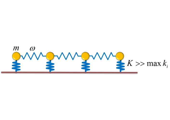
Figure 2.1: Illustration of the model used for deriving the thermal Green’s function of a network of quantum harmonic oscillators.

When the temperature goes to infinity, the inverse temperature $\beta\rightarrow 0$, which means that every edge in the graph vanishes and the resulting graph is trivial, similar to a system of free particles. When the temperature goes to zero, the inverse temperature $\beta\rightarrow\infty$ indicating that an infinity number of edges are created between every pair of nodes connected in $\varGamma$; a situation analogous to a rigid solid.

3 Melting phase transition

Let us consider a connected graph with eigenvalues ordered as $\lambda_{1}>\lambda_{2}\geq\lambda_{3}\geq...\geq\lambda_{n}$. Let us then write the communicability function in the following way

$$G_{pq}(\beta) = e^{\beta\lambda_{1}}\psi_{1}\left(p\right)\psi_{1}\left(q\right)+\left[\sum_{2\leq j\leq n}e^{\beta\lambda_{j}}\psi_{j}^{+}\left(p\right)\psi_{j}^{+}\left(q\right)+\sum_{2\leq j\leq n}e^{\beta\lambda_{j}}\psi_{j}^{-}\left(p\right)\psi_{j}^{-}\left(q\right)\right]$$

$$+\left[\sum_{2\leq j\leq n}e^{\beta\lambda_{j}}\psi_{j}^{+}\left(p\right)\psi_{j}^{-}\left(q\right)+e^{\beta\lambda_{j}}\psi_{j}^{-}\left(p\right)\psi_{j}^{+}\left(q\right)\right],$$

where $\psi_{j}^{+}\left(p\right)$ ($\psi_{j}^{-}\left(p\right)$) means that the $p$th entry of the $j$th eigenvector is positive (negative). Let us consider the graph illustrated in Figure 3.1, where we show the corresponding eigenvectors of the adjacency matrix in a schematic way. The negative entries of the corresponding eigenvectors are illustrated like “vibrations” in the negative direction of the $y$- axis. Similarly for the positive entries, which are represented as vibrations in the positive direction of the $y$- axis. The magnitude of the vibrations are not represented for the sake of simplicity. The term $e^{\beta\lambda_{1}}\psi_{1}\left(p\right)\psi_{1}\left(q\right)$ represents the coordinated vibration of all nodes in the graph at the corresponding value of $\beta$ (see Fig. 3.1), i.e., a translational motion of the whole network. Then, we obtain the purely vibrational term for the pairs of nodes as: $\varDelta G_{pq}\left(\beta\right)=G_{pq}\left(\beta\right)-e^{\beta\lambda_{1}}\psi_{1}\left(p\right)\psi_{1}\left(q\right)$, which can also be expressed as

$$\varDelta G_{pq}(\beta)=\sum_{j\geq 2}^{in-phase}e^{\beta\lambda_{j}}\psi_{j}\left(p\right)\psi_{j}\left(q\right)-\left|\sum_{j\geq 2}^{out-of-phase}e^{\beta\lambda_{j}}\psi_{j}\left(p\right)\psi_{j}\left(q\right)\right|,$$ (3.1)

where the first term, which can be written as $\sum_{2\leq j\leq n}e^{\beta\lambda_{j}}\psi_{j}^{+}\left(p\right)\psi_{j}^{+}\left(q\right)+\sum_{2\leq j\leq n}e^{\beta\lambda_{j}}\psi_{j}^{-}\left(p\right)\psi_{j}^{-}\left(q\right)$, corresponds to the case when both nodes have the same sign in the corresponding eigenvector, and the second term, which can be written as $\sum_{2\leq j\leq n}e^{\beta\lambda_{j}}\psi_{j}^{+}\left(p\right)\psi_{j}^{-}\left(q\right)+e^{\beta\lambda_{j}}\psi_{j}^{-}\left(p\right)\psi_{j}^{+}\left(q\right)$, accounts for the cases in which the two nodes have different sign in the corresponding eigenvector. We notice that the second term is always negative and we use the modulus of it to express the term $\varDelta G_{pq}(\beta)$ as a difference. $\varDelta G_{pq}(\beta)$ accounts for the difference between the in- and out-of-phase vibrations of the corresponding pair of nodes.

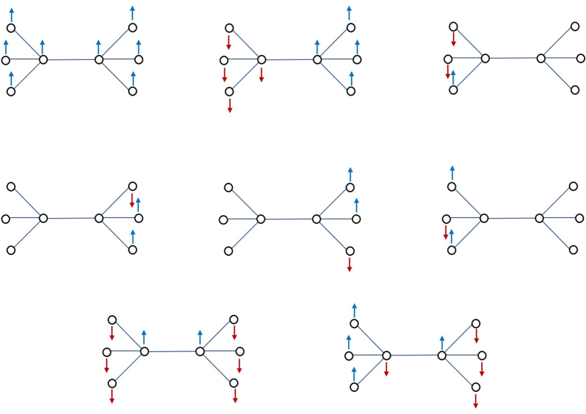
Figure 3.1: Illustration of the sign pattern of the eigenvectors in a simple graph. Only the signs of the eigenvector components are represented by blue (positive) and red (negative) arrows. The magnitudes of the eigenvector components are not represented.

Let us now reconnect with Lindemanncriterion of melting [19] . According to Lindemann the average amplitude of thermal vibrations in crystals increases with the temperature up to a point in which the amplitude of vibration is so large that the atoms invade the space of their nearest neighbors and the melting starts. Lindemann criterion consists in considering that melting might be expected when the mean-square amplitude of vibrations exceed a certain threshold value [19]. Let us consider that in a graph $\Gamma$ such threshold is given by $M(\varGamma,\beta)=\max_{s\neq t\in V}\sum_{j=2}^{n}\psi_{j}\left(s\right)\psi_{j}\left(t\right)e^{\beta\lambda_{j}}$. That is, that melting starts in a given graph when the vibrations of the nodes $p$ and $q$ at a given temperature measured by $\Delta G_{pq}\left(\beta\right)$ exceed the value of the maximum vibration of any pair of nodes in that graph at the same temperature, $M(\varGamma,\beta)$. We should notice that at a given temperature the terms $\varDelta G_{pq}(\beta)$ and $M(\varGamma,\beta)$ may be either positive or negative. Thus, in order to implement the Lindemann criterion on graphs we should sum both terms instead of having their difference,

$$\varDelta\tilde{G}_{pq}(\beta)=M(\varGamma,\beta)+\varDelta G_{pq}(\beta).$$ (3.2)

Then, when $M(\varGamma,\beta)>0$ we have the following scenarios. If $\varDelta G_{pq}(\beta)>0$ then $\varDelta\tilde{G}_{pq}(\beta)$ is always positive as it is the sum of two positive terms indicating a reinforcement of the in-phase vibrations of the two nodes. If $\varDelta G_{pq}(\beta)<0$ then $\varDelta\tilde{G}_{pq}(\beta)>0$ if the difference between the in-phase and out-of-phase vibrations $\varDelta G_{pq}(\beta)$, does not overtake the maximum in-phase vibrations of any pair of nodes in the graph. Otherwise, $\varDelta\tilde{G}_{pq}(\beta)<0$, which indicates that the out-of-phase vibrations of these two nodes have overtaken not only their in-phase vibrations but also the maximum in-phase vibrations of any pair of nodes in the graph. In this last case we will say that the corresponding edge has been melted. On the other hand, when $M(\varGamma,\beta)<0$, then also $\varDelta G_{pq}(\beta)<0$ which means that $\varDelta\tilde{G}_{pq}(\beta)<0$ and the edge necessarily melts. Then, we will call $\varDelta\tilde{G}_{pq}(\beta)$ the graph Lindemann criterion, having in mind that the melting will start when $\varDelta\tilde{G}_{pq}(\beta)<0$. Let us define the following representation of $\varDelta\tilde{G}_{pq}(\beta)$ in the form of a new graph.

Definition 8.

Let $\Gamma=\left(V,E\right)$ be a simple graph. The communicability graph $H\left(V,E^{\prime},\beta\right)$ of $\Gamma=\left(V,E\right)$ is the graph with the same set of nodes as $\Gamma$ and with edge set given by the following adjacency relation

$$A(H,\beta)_{p,q}=\left\{\begin{array}[]{c}\textnormal{1 if }\varDelta\tilde{G}_{pq}(\beta)\geq 0,\\ \textnormal{0 if }\varDelta\tilde{G}_{pq}(\beta)<0.\end{array}\right.$$ (3.3)

In the communicability graph there could be edges connecting pairs of nodes which are not connected in the original graph $\Gamma.$ In a similar way, there could be pairs of nodes not connected in $H\left(V,E^{\prime},\beta\right)$ which correspond to edges in $\Gamma$ (see further example). In other words, $\Gamma$ is not necessarily a subgraph of $H\left(V,E^{\prime},\beta\right)$. For instance, in Fig. 3.2 at $\beta=1$ the two central nodes 1 and 5 of the graph are vibrating out-of-phase. However, because we do not have a temporal sequence of how the vibrations occurs there are also paths connecting 1 and 5 in which all the nodes vibrate in phase. This is the case of the paths 1-2-6-5, 1-4-8-5 and so forth. As a consequence of these paths the nodes 1 and 5 can be vibrating in-phase at some temporal stages of the process. For that reason we introduce the following definitions.

Definition 9.

Let $\Gamma=\left(V,E\right)$ be a simple graph and let $H\left(V,E^{\prime},\beta\right)$ be its communicability graph. Let $p$ and $q$ be two nodes of $\Gamma.$ We say that there is a Lindemann path between the nodes $p$ and $q$ in $\Gamma$ at a given value of $\beta$ if there is a path connecting both nodes in the communicability graph $H\left(V,E^{\prime},\beta\right)$. In this case we say that $\exists L_{p,q}$. Otherwise, we say that $\nexists L_{p,q}$.

We now define a graph that contain all the information about the in- and out-phase nature of the vibrations in a graph $\Gamma=\left(V,E\right)$.

Definition 10.

Let $\Gamma=\left(V,E\right)$ be a simple graph and let $H\left(V,E^{\prime},\beta\right)$ be its communicability graph. The Lindemann graph $F\left(V,E^{\prime\prime},\beta\right)$ of $\Gamma$ is the graph with the same set of vertices as $\Gamma$ and edge set defined by the following adjacency relation

$$A(F,\beta)_{p,q}=\left\{\begin{array}[]{c}\textnormal{1 if $\left(p,q\right)\in E$ and $\exists L_{p,q}$},\\ \textnormal{0 if $\left(p,q\right)\notin E$ or $\nexists L_{p,q}$}.\end{array}\right.$$ (3.4)

To illustrate the previously defined concepts we return to the tree with eight nodes and degree sequence 4,4,1,1,1,1,1,1 at different values of $\beta$ illustrated in Fig. 3.2. For $\beta=1$ the communicability graph has many more edges than the original tree $\Gamma,$ but it also misses the central link connecting the nodes 1 and 5. When constructing the Lindemann graph we should observe that there is a path between every pair of nodes in the corresponding communicability graph, i.e., it is connected. Thus, the Lindemann graph consists of the same set of edges as the original graph. The Lindemann graph is represented by solid lines in the right panels of Fig. 3.2. When $\beta=0.5$ the communicability graph consists of two cliques of four nodes each. Then, the Lindemann graph consists of all edges of $\Gamma$, except the central edge connecting the nodes 1 and 5, because there is no path connecting the two nodes of degree 4 in the communicability graph. At this value of $\beta$ we can say that the melting of this graph has started because for (at least) one pair of nodes the out-of-phase vibrations have overcome the graph Lindemann criterion. Notice that for $\beta=0.3$ the communicability graph has changed in respect to that for $\beta=0.5$, but the Lindemann graphs are exactly the same due to the double conditions that need to be required for having an edge in these graphs. Finally, when $\beta=0.2$ the communicability graph is formed by 8 isolated nodes and so is the Lindemann graph. At this point there is no communicability between any pair of nodes and the Lindemann graph is the trivial graph. In our physical metaphor, the graph is totally “melted”.

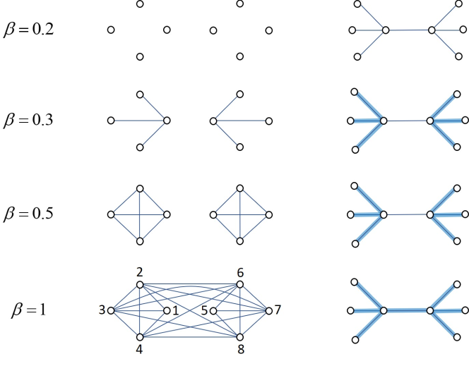
Figure 3.2: Communicability graphs (central panels) at different values of $\beta$ for the tree $\Gamma$ with degree sequence 4,4,1,1,1,1,1,1. In the right panel the edges of the Lindemann graphs are represented as solid lines over the edges of the original graph $\Gamma$.

In the Fig. 3.3 we have plotted the values of $\beta$ versus the number of connected components of the Lindemann graph. At the point $\beta=0.5$, marked in the plot with a fat arrow, there is a transition between a connected to a disconnected Lindemann graph. We have previously identified this value of $\beta=\beta_{c}$ as the melting temperature of this graph. The reader should keep in mind that the physical terms used here represent metaphors from the physical world to a mathematical framework and not a physical reality. The question that immediately emerges here is whether this phase transition is universal for any simple graph or not. In the next section we respond positively to this question.

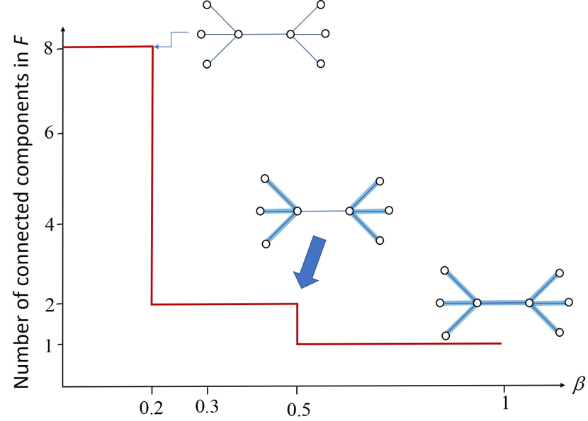
Figure 3.3: Illustration of the transition between connected $\beta>0.5$ to disconnected $\beta\leq 0.5$ Lindemann graph as a function of $\beta$ for the simple tree illustrated in Fig. 3.2.

4 Main result

Here we prove the existence of the phase transition between connected to disconnected Lindemann graph for any simple graph. For proving this result it is enough to prove that this transition occurs in the communicability graph. Then, when the communicability graph is connected also is the Lindemann graph, due to the fact that there is a path between every pair of nodes in a connected graph. In the same way, if the communicability graph is disconnected also is the Lindemann graph because there will be pairs of adjacent nodes of the original graph for which there are no paths connecting them in the communicability graph. We divide our result into two parts. The first deals with all graphs which are not complete multipartite ones. The second proves the result for this kind of graphs.

Theorem 11.

Let $H(\varGamma,\beta)$ be the communicability graph for a non complete multipartite graph $\Gamma=\left(V,E\right).$ Then, there exist a value $\beta_{c}\in[0,\infty)$ such that

(i) $H\left(\varGamma,\beta\geq\beta_{c}\right)$ is connected;

(ii) $H\left(\varGamma,\beta<\beta_{c}\right)$ is disconnected.

Proof.

We start by proving that the communicability graph $H(\varGamma,\beta)$ is disconnected for certain value of the inverse temperature. Then, we prove that it becomes connected for certain value of $\beta$, which immediately implies that the communicability graph $H(\varGamma,\beta)$ makes a transition from connected to disconnected at certain intermediate temperature, which we call $\beta_{c}$. This value is unique since the communicability function is monotonic, as it is the sum of exponential functions which are monotonic. The communicability graph function is

$$\varDelta\tilde{G}_{pq}(\beta):=M(\varGamma,\beta)+\sum_{j=2}^{n}\psi_{j}\left(p\right)\psi_{j}\left(q\right)e^{\beta\lambda_{j}},$$ (4.1)

where $M(\varGamma,\beta)=\max_{s\neq t}\sum\psi_{j}\left(s\right)\psi_{j}\left(t\right)e^{\beta\lambda_{j}}$. Two distinct nodes $p\neq q$ are connected in $H(\varGamma,\beta)$ if $\triangle\tilde{G}_{pq}\geq 0$, and disconnected if $\triangle\tilde{G}_{pq}<0$. Let us consider the case when $\beta\rightarrow 0$. In this case we have $\lim_{\beta\rightarrow 0}\sum_{j=2}^{n}\psi_{j}\left(p\right)\psi_{j}\left(q\right)e^{\beta\lambda_{j}}=\sum_{j=2}^{n}\psi_{j}\left(p\right)\psi_{j}\left(q\right)=-\psi_{1}\left(p\right)\psi_{1}\left(q\right)$. Thus,

$$\triangle\tilde{G}_{pq}\left(\beta\rightarrow 0\right)=-\left(\psi_{1}\left(p\right)\psi_{1}\left(q\right)+\max_{s\neq t}\psi_{1}\left(s\right)\psi_{1}\left(t\right)\right)<0.$$ (4.2)

Then, it is obvious that the edge $pq$ in the graph is disconnected and this happens for every pair of nodes in the graph. Consequently, the communicability graph is disconnected for some $\beta$ when $\beta\rightarrow 0$.

Let us now consider that case when $\beta\rightarrow\infty$. in this case the communicability function $\triangle\tilde{G}_{pq}(\beta)$ is dominated by the term containing the second largest eigenvalue $\lambda_{2}$. Now let $\left(r-1\right)\geq 1$ be the multiplicity of $\lambda_{2}$, i.e., $\lambda_{2}=\lambda_{3}=\cdots=\lambda_{r}$. Then, $\forall p,q\in V,$ we have

$$\triangle\tilde{G}_{pq}(\beta) \rightarrow (\psi_{r}\left(p\right)\psi_{r}\left(q\right)+\psi_{r-1}\left(p\right)\psi_{r-1}\left(q\right)+\ldots+\psi_{2}\left(p\right)\psi_{2}\left(q\right))e^{\beta\lambda_{2}}$$

$$+\max_{s\neq t}\left(\psi_{r}\left(s\right)\psi_{r}\left(t\right)+\psi_{r-1}\left(s\right)\psi_{r-1}\left(t\right)+\ldots+\psi_{2}\left(s\right)\psi_{2}\left(t\right)\right)e^{\beta\lambda_{2}},$$

$$\Rightarrow\triangle\tilde{G}_{pq}(\beta)\rightarrow e^{\beta\lambda_{2}}\sum_{j=2}^{r}\psi_{j}\left(p\right)\psi_{j}\left(q\right)+e^{\beta\lambda_{2}}\max_{s\neq t}\sum_{j=2}^{r}\psi_{j}\left(s\right)\psi_{j}\left(t\right),$$ (4.3)

where $\psi_{2},\psi_{3},\ldots,\psi_{r-1},\psi_{r}$, are the eigenvectors corresponding to the eigenvalue $\lambda_{2}$.
If $\cap_{j=2}^{r}\mathcal{O}(\psi_{j})\neq\emptyset$, then by Lemma 2, one of the following two separate cases hold.

1. No edge in the original graph $\varGamma=\left(V,E\right)$ joins a vertex of $\text{$\mathcal{P}$}\left(\psi_{j}\right)$ to one of $\mathcal{N}\left(\psi_{\mathnormal{j}}\right)$. Then $\psi_{j}\left(p\right)\psi_{j}\left(q\right)\geq 0$, $\forall j\in\{2,3,\ldots,r\},$ and $\forall(p,q)\in E$, $\triangle\tilde{G}_{pq}$ (4.3) satisfies:
   

   $$\triangle\tilde{G}_{pq}(\beta)\geq 0.$$ (4.4)

   Now let us rewrite the function $\triangle\tilde{G}_{pq}$ in the following form, where $s$ and $t$ are two distinct nodes in the graph:

   $$\triangle\tilde{G}_{pq}=\left(\exp\left(\beta A\right)\right){}_{pq}-\psi_{1}\left(p\right)\psi_{1}\left(q\right)e^{\beta\lambda_{1}}+\max_{s\neq t}\left[\left(\exp\left(\beta A\right)\right){}_{st}-\psi_{1}\left(s\right)\psi_{1}\left(t\right)e^{\beta\lambda_{1}}\right].$$

   Let us now consider $\beta=0$, then $\forall p\neq q\in V,$
   

   $$\triangle\tilde{G}_{pq}=-\psi_{1}\left(p\right)\psi_{1}\left(q\right)+\max_{s\neq t}\left[-\psi_{1}\left(s\right)\psi_{1}\left(t\right)\right]<0,$$ (4.5)

   since the leading eigenvector $\vec{\psi}_{1}$ can be chosen such that its components $\mathbf{\mathbf{\psi}}_{1}(p)$ are positive for all $p\in V$ according to the Perron-Frobenius theorem. The exponential matrix $\exp(0\cdot A)=I$, so that $(\exp(\beta A))_{pq}=0$, $\forall p\neq q\in V.$ Then, from 4.4 and 4.5, we have that there is a value of $\beta_{c}\in[0,\infty),$ such that $H\left(\varGamma,\beta\geq\beta_{c}\right)$ is connected and $H\left(\varGamma,\beta<\beta_{c}\right)$ is disconnected.
   

2. There exists at least one edge that joins a vertex of $\text{$\mathcal{P}$}(\psi_{j})$ to one of $\mathcal{N}$($\psi_{j}$), moreover $\left\langle\text{$\mathcal{P}$}(\psi_{j})\right\rangle$ and $\left\langle\text{$\mathcal{N}$}(\psi_{j})\right\rangle$ are connected.
   Let $p\in\cap_{j=2}^{r}\mathcal{O}(\psi_{j})$, then $\psi_{j}\left(p\right)=0$, $\forall j\in\{2,3,\ldots,r\}.$ Then $\forall q\neq p\in V,$ we get:

   $$e^{\beta\lambda_{2}}\sum_{j=2}^{r}\psi_{j}\left(p\right)\psi_{j}\left(q\right)=0,$$

   and
   

   $$\triangle\tilde{G}_{pq}(\beta)\geq 0.$$ (4.6)

   Therefore all the nodes of $V$ are connected to each other through $p$. Then from 4.5, and 4.6, we have that there is $\exists\beta_{c}\in[0,\infty),$ such that $H\left(\varGamma,\beta\geq\beta_{c}\right)$ is connected and $H\left(\varGamma,\beta<\beta_{c}\right)$ is disconnected.

Now let us consider the case in which $\cap_{j=2}^{r}\mathcal{O}(\psi_{j})=\emptyset$. Let $p\in\text{$\mathcal{P}$(}\psi_{j})\cup\mathcal{O}(\psi_{j})$ (resp., $p\in\text{\text{$\mathcal{N}$}(}\psi_{j}))$ $j\in\{2,3,\ldots,r\}$. Then according to Lemma 3, there exists $q\in\text{$\mathcal{P}$(}\psi_{j})\cup\mathcal{O}(\psi_{j})$ (resp., $q\in\text{\text{$\mathcal{N}$}(}\psi_{j}))$ such that $(p,q)\in E$ and either $p,q\in\text{$\mathcal{P}$(}\psi_{j})\cup\mathcal{O}(\psi_{j})$ or $\text{$\mathcal{N}$}(\psi_{j})$, $\forall j\in\{2,\ldots,r\}$. It holds that $\psi_{j}\left(p\right)\psi_{j}\left(q\right)\geq 0$, $\forall j$ such that we get:

$$\sum_{j=2}^{r}\psi_{j}\left(p\right)\psi_{j}\left(q\right)\geq 0,$$

and

$$\triangle\tilde{G}_{pq}(\beta)\geq 0.$$ (4.7)

Now, since there are $(r-1)$ eigenvectors corresponding to the eigenvalue $\lambda_{2}$, there are $2^{r-1}$ of intersected subsets in $V$ of $\text{$\mathcal{P}$(}\psi_{j})\cup\mathcal{O}(\psi_{j})$ and $\text{$\mathcal{N}$}(\psi_{j})$. In these sets the nodes have the same sings of the eigenvector components $\psi_{j}$, $\forall j\in\{2,3,\ldots,r\}.$ Let us denote these subsets by $W_{1},W_{2},\cdots,W_{2^{r-1}}$ ( When $r-1=2$ these subsets are: $W_{1}=(\text{$\mathcal{P}$(}\psi_{2})\cup\mathcal{O}(\psi_{2}))\cap(\text{$\mathcal{P}$(}\psi_{3})\cup\mathcal{O}(\psi_{3}))$, $W_{2}=\text{($\mathcal{P}$(}\psi_{2})\cup\mathcal{O}(\psi_{2}))\cap\text{$\mathcal{N}$}(\psi_{3})$, $W_{3}=\text{$\mathcal{N}$}(\psi_{2})\cap\text{($\mathcal{P}$(}\psi_{3})\cup\mathcal{O}(\psi_{3}))$ and $W_{4}=\text{$\mathcal{N}$}(\psi_{2})\cap\text{$\mathcal{N}$(}\psi_{3})$). Then $\forall p,q\in W_{h}$, $\forall h\in\{1,2,\ldots,2^{r-1}\}$, it holds $\psi_{j}\left(p\right)\psi_{j}\left(q\right)\geq 0$, $\forall j$ and $\triangle\tilde{G}_{pq}(\beta)\geq 0.$ So that the supgraph $\left\langle W_{h}\right\rangle$, $\forall h\in\{1,2,\ldots,2^{r-1}\}$, is connected.

Proof.

Finally, we need to show whether the subgraphs $\left\langle W_{1}\right\rangle,\left\langle W_{2}\right\rangle,\cdots,\left\langle W_{2^{r-1}}\right\rangle$ are connected to each other, such that we get a connected graph. Let $p^{\prime}\in\left\langle W_{h}\right\rangle$ and $q^{\prime}\in\left\langle W_{s}\right\rangle$, where $h,s\in\{1,2,\ldots,2^{r-1}\}$, such that the absolute value of $\sum_{j=2}^{r}\psi_{j}\left(p^{\prime}\right)\psi_{j}\left(q^{\prime}\right)$, satisfies:

$$\sum_{j=2}^{r}\psi_{j}\left(p^{\prime}\right)\psi_{j}\left(q^{\prime}\right)\leq\max_{s\neq t\in V}\sum_{j=2}^{r}\psi_{j}\left(s\right)\psi_{j}\left(t\right),$$

Then $\triangle\tilde{G}_{p^{\prime}q^{\prime}}$ (4.3) satisfies:

$$\triangle\tilde{G}_{p^{\prime}q^{\prime}}(\beta)\geq 0,$$ (4.8)

therefore $\left\langle W_{1}\right\rangle,\left\langle W_{2}\right\rangle,\cdots,\left\langle W_{2^{r-1}}\right\rangle$ are connected to each other. Then from 4.5, 4.7 and 4.8 we have there is $\beta_{c}\in[0,\infty),$ such that $H\left(\varGamma,\beta\geq\beta_{c}\right)$ is connected and $H\left(\varGamma,\beta<\beta_{c}\right)$ is disconnected, which finally proves the result. ∎

∎

Remark 12.

In the case of complete multipartite graphs which were not included in the Theorem 11 we have the following. As in the general case $\varDelta\tilde{G}_{pq}(\beta\rightarrow 0)<0$, which indicates that the edge does not exist, and this is true for any pair of nodes in the graph. Then, we have to show when such edge exists. According to Lemma 1 [29] in complete multipartite graphs $\lambda_{2}\leq 0$. Then, let us first consider the case when $\lambda_{2}=0$. In this case when $\beta\rightarrow\infty$, the communicability function $\triangle\tilde{G}_{pq}(\beta)$ is dominated by the term of the largest eigenvalue $\lambda_{2}$. Now let $\left(r-1\right)\geq 1$ be the multiplicity of $\lambda_{2}$, i.e., $\lambda_{2}=\lambda_{3}=\cdots=\lambda_{r}$. Then $\forall p,q\in V,$

$$\triangle\tilde{G}_{pq}(\beta) \rightarrow e^{\beta\lambda_{2}}\sum_{j=2}^{r}\psi_{j}\left(p\right)\psi_{j}\left(q\right)+e^{\beta\lambda_{2}}\max_{s\neq t\in V}\sum_{j=2}^{r}\psi_{j}\left(s\right)\psi_{j}\left(t\right),$$

which implies that

Remark 13.

$$\triangle\tilde{G}_{pq}(\beta)\rightarrow\sum_{j=2}^{r}\psi_{j}\left(p\right)\psi_{j}\left(q\right)+\max_{s\neq t\in V}\sum_{j=2}^{r}\psi_{j}\left(s\right)\psi_{j}\left(t\right),$$ (4.9)

since $e^{\beta\lambda_{2}}=1$. So that the proof for the case when $\cap_{j=2}^{r}\mathcal{O}(\psi_{j})\neq\emptyset$, will be the same as that for the case when $\lambda_{2}>0$, which is the Case 2, in Theorem 10.
Now when $\cap_{j=2}^{r}\mathcal{O}(\psi_{j})=\emptyset$ then for the nodes which belong to the sets $W_{h}$, $\forall h\in\{1,2,\ldots,2^{r-1}\}$, (the sets of all of intersected subsets in $V$ of $\text{$\mathcal{P}$(}\psi_{j})\cup\mathcal{O}(\psi_{j})$ and $\text{$\mathcal{N}$}(\psi_{j})$, $j\in\{2,3,\ldots,r\}$) are connected to each other in $\left\langle W_{h}\right\rangle$, since they have the same sings of the eigenvector components $\psi_{j}$, $\forall j\in\{2,3,\ldots,r\}$. For the nodes which do not belong to $W_{h}$, $\forall h\in\{1,2,\ldots,2^{r-1}\}$, let $p\in V$, $p\notin W_{h}$, $\forall h\in\{1,2,\ldots,2^{r-1}\}$, and let $q\in W_{h}$, such that the absolute value of $\sum_{j=2}^{r}\psi_{j}\left(p\right)\psi_{j}\left(q\right)$, satisfies

$$\left|\sum_{j=2}^{r}\psi_{j}\left(p\right)\psi_{j}\left(q\right)\right|\leq\max_{s\neq t\in V}\sum_{j=2}^{r}\psi_{j}\left(s\right)\psi_{j}\left(t\right),$$

Then $\triangle\tilde{G}_{pq}$ (4.9) satisfies

$$\triangle\tilde{G}_{pq}(\beta)\geq 0.$$ (4.10)

So let us denote the subgraphs generated by $W_{h}$, and the other nodes of $V$ which do not belong to $W_{h}$, by $\left\langle W^{\prime}_{1}\right\rangle,\left\langle W^{\prime}_{2}\right\rangle,\cdots,\left\langle W^{\prime}_{2^{r-1}}\right\rangle$. Finally, in the same previous way we can connect $\left\langle W^{\prime}_{1}\right\rangle,\left\langle W^{\prime}_{2}\right\rangle,\cdots,\left\langle W^{\prime}_{2^{r-1}}\right\rangle$ to each other, such that we get a connected graph. Let $p^{\prime}\in\left\langle W^{\prime}_{h}\right\rangle$ and $q^{\prime}\in\left\langle W^{\prime}_{s}\right\rangle$, where $h,s\in\{1,2,\ldots,2^{r-1}\}$, such that the absolute value of $\sum_{j=2}^{r}\psi_{j}\left(p^{\prime}\right)\psi_{j}\left(q^{\prime}\right)$, satisfies:

$$\left|\sum_{j=2}^{r}\psi_{j}\left(p^{\prime}\right)\psi_{j}\left(q^{\prime}\right)\right|\leq\max_{s\neq t\in V}\sum_{j=2}^{r}\psi_{j}\left(s\right)\psi_{j}\left(t\right),$$

Then $\triangle\tilde{G}_{pq}$ (4.9) satisfies

$$\triangle\tilde{G}_{p^{\prime}q^{\prime}}(\beta)\geq 0.$$ (4.11)

Therefore $\left\langle W^{\prime}_{1}\right\rangle,\left\langle W^{\prime}_{2}\right\rangle,\cdots,\left\langle W^{\prime}_{2^{r-1}}\right\rangle$ are connected to each other. Then from 4.5, 4.10 and 4.11 we have that there is $\beta_{c}\in[0,\infty),$ such that $H\left(\varGamma,\beta\geq\beta_{c}\right)$ is connected and $H\left(\varGamma,\beta<\beta_{c}\right)$ is disconnected.

On the other hand, when $\lambda_{2}<0$ we have that

$$\varDelta\tilde{G}_{pq}(\beta)=\max_{s\neq t}\sum\psi_{j}\left(s\right)\psi_{j}\left(t\right)e^{-\beta\left|\lambda_{j}\right|}+\sum_{j=2}^{n}\psi_{j}\left(p\right)\psi_{j}\left(q\right)e^{-\beta\left|\lambda_{j}\right|}.$$ (4.12)

This means that $\lim_{\beta\rightarrow\infty}\varDelta\tilde{G}_{pq}(\beta)=0$. However, such limit can be either positive–existence of the edge–or negative–not existence of the edge. Thus, in this case we can consider that the edge exists if $\left|\lim_{\beta\rightarrow\infty}\varDelta\tilde{G}_{pq}(\beta)\right|\leq\varepsilon$, where $\varepsilon$ is a threshold very close to zero. The case of complete multipartite graphs is an all-or-nothing case of melting. That is, at $\beta=0$ all the nodes in the Lindemann graph are isolated. When $\beta$ is very large all the nodes in the communicability graph are connected to each other and the Lindemann graph is the same as the original graph. Thus, in these graphs there is not a gradual melting as in the rest of the graphs but an abrupt transition between being connected to fully disconnected occurs.

5 Modeling results

5.1 Melting of granular materials

In this section we study the influence of order and randomness on the melting phase transition in graphs. The influence of order vs. randomness is on the basis of many physical problems. In particular, here we are interested in using graphs as a model of solids and granular materials with ordered structures vs. those having a random one. The classical example of an ordered system is a crystal where atoms or molecules are arranged in a repeating pattern [31]. On the other hand, amorphous solids, which are characterized by the lack of regular pattern or repetition, are good examples of random-like materials [1]. In order to model a random-like material we consider here a type of random graph known as the Gabriel graph [15]. The Gabriel graphs $\Gamma=(V,E)$ are constructed by placing randomly and independently $n$ points in a unit square, then for each pair of points $i\in V$, $j\in V$, $i\neq j,$ constructs a disk in which the line segment $\overline{ij}$ is a diameter (see Fig. 5.1 (left panel)). The two points will be connected if the corresponding disk does not contain any other element of $V$. An example of Gabriel graph is given in Fig. 5.1 (Right panel).

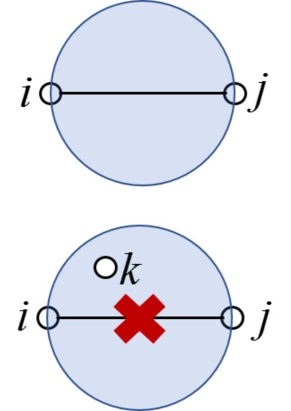
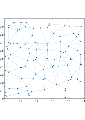
Figure 5.1: Illustration of the construction process of a Gabriel graph (left), where a disk is defined for a pair of nodes which forms a diameter of the disk. Because there is no point inside that disk the two nodes are connected (top graphic). In the bottom graphic a point $k$ is inside the disk and the two nodes $i$ and $j$ are not connected. (right panel) An example of a Gabriel graph with $n=100$ nodes.

The reason why we consider random neighborhood (Gabriel) graphs here instead of other types of random graphs is the following. To keep the analogy with solid materials we should maintain certain geometric disposition of the nodes. This geometric arrangements of nodes are possible in the so-called random geometric graphs (RGGs) as well as in the random neighborhood graphs (RNGs). The RGGs are nonplanar graphs, which implies that node $A$ can interact with another $B$ even in the case that a third node $C$ is exactly in the middle between $A$ and $B$. This, of course, is not a realistic scenario for the interaction between atoms or molecules and not appropriate for representing a solid. However, Gabriel graphs are planar graphs and avoid the interaction between mutually occluded nodes. Consequently, they are appropriate to model amorphous solids.

The differences in the ordered vs. random arrangement of atoms/molecules in crystalline and amorphous solids make that they differ significantly in the way they change their phase from solid to liquid. That is, a fundamental difference between crystalline and amorphous solids resides in the way they melt. While a crystalline solid has a sharp transition from solid to liquid, the amorphous solid does not. Instead, it displays a very smooth transition for a long range of temperatures. The second characteristic feature is that for the same material in amorphous and crystalline forms, the amorphous one melts at higher temperature than the crystalline one. For instance, crystalline quartz melts at $1,550\textdegree C$ and amorphous quartz melts in the range $1,500-2000\textdegree C$. We are interested in investigating here this physical reality as an analogy for our crystalline and amorphous graphs.

In Fig. 5.2 we illustrate the plot of the change in the number of connected components in the communicability graph with the change of $\beta$ for a $10\times 10$ square grid and a Gabriel graph with $n=100$ nodes and $m=180$ edges. Similar results to the ones presented here were obtained for triangular and hexagonal lattices (results not shown). That is, the main difference between these two kinds of graphs resides only in the order/randomness of the nodes in a unit square. The lattice representing a crystalline graph and the Gabriel graph representing an amorphous one. The main observation is that while the crystalline graph displays a sharp increase in the number of connected components with the decrease of $\beta$, the amorphous one displays a rather slow change (notice that the $x$-axis is in logarithmic scale). The second important observation is that the structure of the crystalline graph is destroyed more quickly than that of the amorphous one. For instance, if we consider the value of $\beta$ at which the number of connected components is exactly half the number of nodes, we can see that the crystalline graph reaches that point an order of magnitude before than the amorphous one. If we identify this value of $\beta$ as the melting temperature of a graph we can say that the crystalline graph has a melting temperature one order of magnitude smaller than that of an amorphous one. We repeated the experiment with a $25\times 25$ square lattice and the corresponding Gabriel graph to see whether there are some small size effects and observed that the results are very much the same, although we have increased the size of the graphs by a factor of 6 (results not shown).

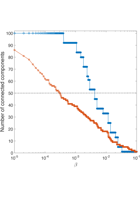
Figure 5.2: Change of the number of connected components in the Lindemann graph for the $10\times 10$ square grid (circles) and Gabriel graph with $n=100$ nodes and $m=180$ edges (squares). The results for the Gabriel graphs are the average of 100 random realizations.

Another possibility of the current approach is that it allows us to visualize the evolution of the “melting” process in graphs in order to gain insights about its mechanism. In Fig. 5.2 we illustrate some snapshots of the change in the communicability structure with the change of $\beta$ for the square lattice. We represent in red the nodes that have removed all of their edges and are now disconnected from the giant connected component. In blue we represent those nodes which form the giant connected component of the graph.

At very low values of $\beta$, e.g. $\beta=0.000025$ (Fig. 5.3 (c)) the communicability structure of the lattice resembles a trivial graph in which almost every node is isolated. As the temperature drops, $\beta$ increases, certain structures start to emerge. In particular, for $\beta=0.0005$ (Fig. 5.3 (b)) an annulus–external part of the lattice–is solidified into a single connected component and only the central part of the graph remains melted. As the temperature drops below $\beta=0.000075$ (Fig. 5.3 (a)), the melted region–red nodes–shrinks to the very center of the lattice. The observed pattern of melting of the square lattice is similar to the one observed experimentally for crystalline solids. In Fig. (Fig. 5.3 (d)) we illustrate the results of Wang et al. [33] for the melting of colloidal crystals which show such patter of central melting.

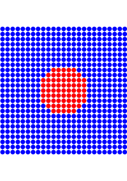
(a)

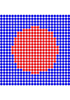
(b)

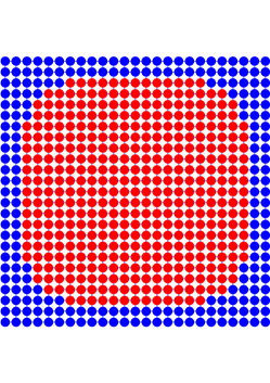
(c)

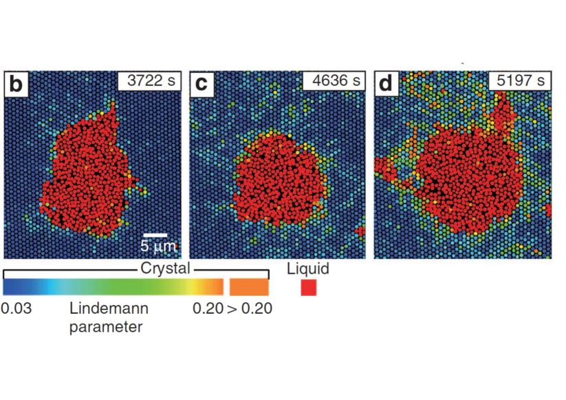
(d)

Figure 5.3: Illustration of the melting of a $25\times 25$ square lattice at $\beta=0.000075$ (a), $\beta=0.00005$ (b) and $\beta=0.000025$ (c). Results for the melting of colloidal crystals obtained by Wang et al. [33]. In plots (a)-(c) the nodes not in the giant connected component are colored in red.  

In the case of the amorphous graph there is no repeating pattern in them, and it is impossible to find a general structural pattern of the evolution of the melting process. A few snapshots of the process are given in Fig. 5.4. The temperature needed to melt these graphs is significantly higher–smaller $\beta$–than the ones needed to melt square lattices of the same size, which coincides with our previous observations as well as with the experimental results for crystalline and amorphous solids. The reasons of this significant difference will become clear in the next section of this work.

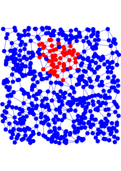
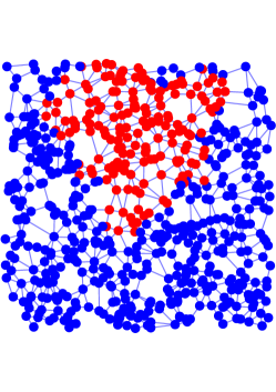
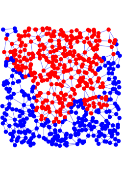
Figure 5.4: Nodes in each of the connected components of the Gabriel graph studied here for $\beta=10^{-8}$, $10^{-9}$ and $10^{-10}$ from left to right. The nodes not in the giant connected component are colored in red.

5.2 Complex networks

The term complex networks is frequently used to refer to graphs representing the skeleton of complex systems, such as social, ecological, infrastructural, technological and biomolecular networks [9]. Here we consider a series of 47 complex networks–see Supplementary Information for description and references–arising from these different scenarios. Here we split our analysis into two parts. First we consider global properties of the networks and then we analyze the influence of node-level centrality on the melting process of these networks.

5.2.1 Global analysis

We start here by finding the value of $\beta$ at which the transition between connected to disconnected Lindemann graph occurs. Our first task is to relate the values of $\beta_{c}$ to some simple topological parameters of the networks in order to understand the structural dependence of this transition. With this goal we study the following structural representative parameters of networks: edge density $\delta$, average degree $\bar{k}$, maximum degree $k_{max}$, average Watts-Strogatz clustering coefficient $\bar{C}$, average path length $\bar{l}$, shortest path efficiency $E$, spectral radius of the adjacency matrix $\lambda_{1}$, second largest eigenvalue of the adjacency matrix $\lambda_{2}$, spectral gap of the adjacency matrix $\Delta$, average communicability distance $\bar{\xi}$, average resistance distance $\bar{\Omega}$, and average communicability angles $\bar{\theta}$. The definitions of these measures are given in the Supplementary Information accompanying this work. We investigate correlations between these measures and the values of $\beta_{c}$ for the 47 networks studied here in linear, semi-log and logarithmic scales. The most significant correlation was obtained for $\ln\beta_{c}$ and $\ln\delta$ ($r=0.79),$ where $r$ is the Pearson correlation coefficient. Also significant are the correlations between $\ln\beta_{c}$ and $\bar{l}$ ($r=-0.72),$ and with $\ln E$ ($r=0.72$).

The correlations found for $\ln\beta_{c}$ with some of the previous structural parameters may be hiding something about the real structural characteristic of networks that influence their “melting”. For instance, the negative correlation between edge density and $\beta_{c}$ seems suspicious. Our intuition tells us that, under all other structural conditions the same, high density networks should melt at higher temperatures, i.e., lower $\beta_{c}$, than lower density ones. This is exactly what it is observed in molecular crystals of nonpolar molecules, such as linear alkanes [3]. In addition, in the previous section we have studied two different kinds of networks which differ very significantly in theirs values of $\beta_{c}$ in spite of the fact that they have exactly the same number of nodes and edge densities. While the square lattice is an almost regular graph, in a Gabriel graph there are small degree heterogeneities that emerge from the clustering of groups of nodes in a relatively close space. Then, the fact that smaller and denser (real-world) networks are the ones having the largest $\beta_{c}$, i.e., they have Lindemann graphs easier to disconnect, may indicate that the “degree homogeneity” of these networks more than their sizes or densities is the real driver of their melting. In order to capture these degree irregularities we recall the definition of the average degree of a network

$$\bar{k}=\dfrac{2m}{n}=\dfrac{\vec{1}^{T}A\vec{1}}{\vec{1}^{T}\vec{1}}.$$ (5.1)

The right-hand side of the previous equation is useful to think that the spectral radius of the adjacency matrix is a sort of average degree, which instead of counting only the number of nearest neighbors of a node consider also a more global picture around it

$$\lambda_{1}=\dfrac{\vec{\psi}_{1}^{T}A\vec{\psi}_{1}}{\vec{\psi}_{1}^{T}\vec{\psi}_{1}}.$$ (5.2)

Notice that $\bar{k}\leq\lambda_{1}$ with equality if and only if the graph is regular. Thus, the term $\left(\lambda_{1}/\bar{k}\right)$ represents the ratio of a more global environment of a node to its more local one. That is, the ratio $\left(\lambda_{1}/\bar{k}\right)$ indicates how a node “sees” as average its global environment in relation to its nearest neighbors. In a regular graph its local environment, i.e., its degree, is identical to the degree of its neighbors, second neighbors, and so on and we get that $\left(\lambda_{1}/\bar{k}\right)$=1. Then, we can define the following index of global to local degree heterogeneity

$$\varrho\left(G\right)=n\left(\dfrac{\lambda_{1}}{\bar{k}}\right).$$ (5.3)

Notice that $\varrho\left(G\right)=\left(\dfrac{\lambda_{1}}{\delta}\right)$, which may explain the previously observed correlation between $\ln\beta_{c}$ and $\ln\delta$. We have then used $\varrho\left(G\right)$ as an indicator of the global to local heterogeneity of the 47 real-world networks analyzed here. In Fig. 5.5 we illustrate the log-log plot of $\varrho\left(G\right)$ versus $\beta_{c}$, which has correlation coefficient $r=-0.85$. The values of $\varrho\left(G\right)$ also explain the differences in the melting of the square lattice ($\varrho\left(G\right)\approx 641.89$) and the Gabriel graphs ($\varrho\left(G\right)\approx 780.62$) studied in the previous section.

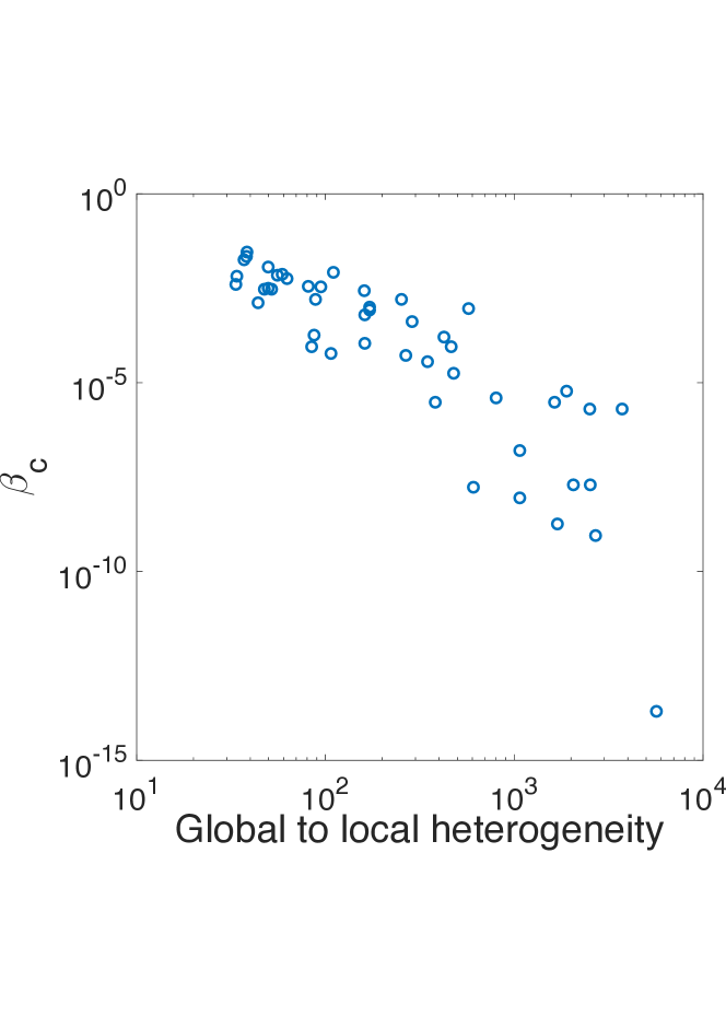
Figure 5.5: Changes of $\beta_{c}$ for 47 real-world networks as a function of their global/local degree heterogeneity as described in this work.

The most important message of this section is the following. The disconnection of the Lindemann graph of a given graph, i.e., its melting, depends very much on the differences between global and local degree heterogeneities. Regular graphs are easier to melt than nonregular ones, and the more irregular–in terms of global to local degree heterogeneity–the graph is the smallest the value of $\beta_{c}$, i.e., more difficult to melt.

5.2.2 Local analysis

In this subsection we are interested in the local analysis of the effects of decreasing the value of $\beta$ on the topological structure of a network. In particular we investigate computationally two important aspects of the graph melting process: (i) How the nodes of a network melt? and (ii) Which structural parameter drives the melting of the nodes? For investigating these questions we consider a subset of the real-world networks studied in this work. We create a melting barcode plot in which we plot every node in the $y$-axis and in the $x$-axis we provide the value of $\beta$ at which the corresponding node disconnect from the giant connected component of the graph. In Fig. 5.6 we illustrate the melting barcodes of three networks: neurons (a), Little Rock (b) and corporate elite (c). We need to read these melting barcodes from right to left as the melting process starts at higher values of $\beta$ and proceed by decreasing it. There are significant differences in the three barcodes presented which point out to the differences existing in the melting processes of the different graphs analyzed. First, we can observe that the shape of the melting barcodes are different. While in “neurons” the decay resembles an exponential curve, in “Little Rock” it is almost linear and in the “corporate elite” it displays a more skewed shape (see further for quantitative analysis). In the second place, the barcodes of “Little Rock” and of corporate elite display regions in which large groups of nodes are disconnected at the same temperature, while in neurons the change is smoother.

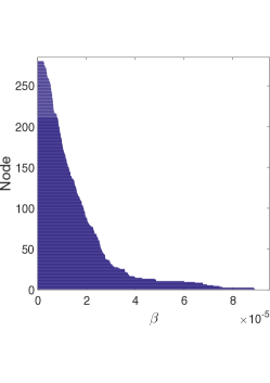
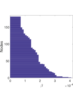
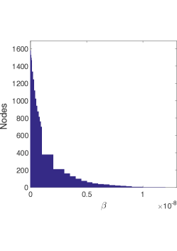
Figure 5.6: Illustration of the melting barcodes of the networks of neurons (a), Little Rock (b) and corporate elite (c).

We then investigate the rate of change of the melting process in the networks analyzed by considering the shape of the histogram of the number of nodes “melted” at a given temperature. That is, we construct the histograms of the number of nodes melted in a temperature range versus the range of temperatures. In general we observe two kinds of decay of the number of nodes melted at a given temperature in relation to the inverse temperature. They are:

$$\eta=a\exp\left(\zeta\cdot\beta\right),$$ (5.4)

$$\eta=b\cdot\beta^{\gamma},$$ (5.5)

where $\eta$ is the number of nodes melted at a given value of $\beta$. For some of the smallest networks it was not possible to find any particular law of the decay of $\eta$ as a function of $\beta$. These were the cases of the networks of Benguela ($n=29$), Coachella ($n=30$), Social3 ($n=32$), St. Marks ($n=48$), as well as for the network of Little Rock, which is not so small ($n=181$) but it also has a very disperse histogram. For the rest of the networks analyzed we display the parameters of the fitting to Eqs. 5.4 and 5.5 in Table 1.

network	Eq. 5.4			network	Eq. 5.5
	$a$	$\zeta$	$r^{2}$		$b$	$\gamma$	$r^{2}$
Prison	$24.58$	$-1.858\cdot 10^{-3}$	$0.790$	Macaque	$5.59\cdot 10^{-15}$	$-6.953$	$0.756$
Neurons	$178$	$-6.032\cdot 10^{-4}$	$0.975$	Stony	$4.84\cdot 10^{-12}$	$-3.515$	$0.887$
Small World	$334.9$	$-1.06\cdot 10^{-4}$	$0.995$	PIN B. subtilis	$2.34\cdot 10^{-3}$	$-1.016$	$0.976$
Ythan	$91.82$	$-3.61\cdot 10^{-3}$	$0.965$	Roget	$5.40\cdot 10^{-8}$	$-1.441$	$0.992$
Electronic 1	$75.87$	$-5.99\cdot 10^{-4}$	$0.934$	Software_Abi	$7.05\cdot 10^{-17}$	$-2.621$	$0.999$
PIN H. pylori	$1233$	$-2.89\cdot 10^{-6}$	$0.999$	Corporate elite	$9.96\cdot 10^{-14}$	$-1.744$	$0.999$

Table 1: Values of the fitting parameters for the Eqs. 5.4 and 5.5 displaying the relation between the number of nodes melted at a given value of $\beta$ as a function of $\beta$ for several real-world networks.

The fitting parameters given in Table 1 indicate the differences in the rates of melting of the networks analyzed. These rates of melting represent a new measure of the robustness of networks to the effects of external stresses to which the networks are submitted to, as accounted for by the inverse temperature. For instance, those networks melting according to Eq. 5.4 are more robust to external stresses than the ones melting according to Eq. 5.5. In comparing those networks that melt exponentially with $\beta$ it is clear that the social network of inmates in prison (Prison) and the food web of Ythan are significantly less robust to such external stresses than the protein interaction network of H. pylori. The network representing the visual cortex of macaque melts very quickly in relation to the rest of the networks analyzed indicating that once the external stress has trigger the melting process the nodes of this network disconnect very fast from the giant connected component.

Finally, we investigate which structural parameters determine the melting process of the nodes of a network. In particular we consider here the role of node centrality on the melting of the corresponding node. We then analyze the relation between the value of $\beta$ at which a node melts and its degree (DC), closeness (CC), betweenness (BC), eigenvector (EC) and subgraph centrality (SC). All these measures are defined in the Supplementary Information. In general, we observe that the values of $\beta$ at which the nodes melt correlate very well with EC. All networks studied displayed Pearson correlation coefficients between these two parameters higher than $0.90$, with the exceptions of the networks of Benguela and Macaque visual cortex. In addition we investigate the coefficient of variation (CV) of the values of $\beta$ at which a node melts estimated from a linear regression with EC. This coefficient is given by the standard deviation of the estimate divided by the mean of the values of $\beta$ at which the nodes melt in a given network. Here we provide the values of both Pearson correlation coefficient and CV in percentage for the networks investigated: Benguela ($r=0.68$, 34.3%), Coachela ($r=0.93$, 15.1%), Social3 ($r=0.95$, 16.2%), Macaque ($r=0.82$, 19.8%), St. Marks ($r=0.97$, 11.7%), Prison ($r=0.998$, 3.9%), PIN B. subtilis ($r=0.999$, 3.4%), Stony ($r=0.94$, 13.8%), Electronic1 ($r=0.99999$, 0.4%), Ythan1 ($r=0.99$, 8.6%), Small World ($r=0.998$, 5.0%), Little Rock ($r=0.989$, 6.9%), Neurons ($r=0.999$, 1.3%), Roget ($r=0.997$, 7.6%), PIN H. pylori ($r=0.997$, 7.6%), Software Abi ($r=0.996$, 19.7%), Corporate elite ($r=0.99$, 18.1%). An important point to have into account here is that although the correlation coefficients are in general very high, the values of CV indicate that the correlations are characterized by certain levels of dispersion. For instance, the networks of Software Abi and the Corporate elite have CV close to 20% although they have correlation coefficients larger than 0.99.

In general, we observe that when $\beta_{c}$ is arbitrarily small, the correlation between the value of $\beta$ at which the node melts and EC is better than when $\beta_{c}$ is relatively large, e.g. Benguela, Coachela, Social3, Macaque, St. Marks, etc. The reason for that difference is the following. Let us recall that at $\beta_{c}$ the value of the Lindemann criterion is negative, that is

$$\Delta\tilde{G}_{pq}\left(\beta_{c}\right)=\sum_{j=2}^{n}\psi_{j}\left(p\right)\psi_{j}\left(q\right)e^{\beta\lambda_{j}}<0.$$ (5.6)

Let $\beta_{c}$ be arbitrarily small such that we have $e^{\beta_{c}\lambda_{j}}\approx 1$ for all $j$ and

$$\begin{split}-\left|\Delta\tilde{G}_{pq}\left(\beta_{c}\right)\right|&=M\left(\Gamma,\beta_{c}\right)+\sum_{j=2}^{n}\psi_{j}\left(p\right)\psi_{j}\left(q\right)\\ &=M\left(\Gamma,\beta_{c}\right)-\psi_{1}\left(p\right)\psi_{1}\left(q\right),\end{split}$$ (5.7)

where $M\left(\Gamma,\beta_{c}\right)$ is obviously a constant. Then, if we take the sum of all the values of $\Delta\tilde{G}_{pq}\left(\beta_{c}\right)$ for the node $p$ we have

$$\begin{split}-\sum_{q\neq p}\left|\Delta\tilde{G}_{pq}\left(\beta_{c}\right)\right|&=M\left(\Gamma,\beta_{c}\right)-\psi_{1}\left(p\right)\sum_{q\neq p}\psi_{1}\left(q\right)\end{split}$$ (5.8)

which clearly explains the observed high positive correlation between the values of $\beta$ at which a node melts and $\psi_{1}\left(p\right)$ for networks having $\beta_{c}$ very close to zero. Also, it explains why those networks for which $\beta_{c}$ is not sufficiently small display bad correlations between the values of $\beta$ at which a node melts and $\psi_{1}\left(p\right)$.

This result has important consequences for the robustness of networks. Those networks displaying a high robustness to external stresses, such that $\beta_{c}$ is very close to zero, start their melting by the most central nodes according to EC. That is, if we consider a network like the USA transportation network, which has $\beta_{c}$ of the order of $10^{-7},$ we will observe that the first airports to be disconnected from the giant connected component are the most important ones in terms of their connectivity. Here we give the list of the first airports separated from the giant connected component in order of their disconnection: Chicago O’Hare, Dallas/Forth Worth Int., The William B. Hartsfield (Atlanta), Detroit Metropolitan, Pittsburgh Intel., Lambert-St. Louis, Charlotte/Douglas Int. (see Fig. 5.7).

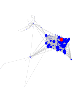
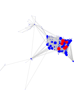
a) b) c)

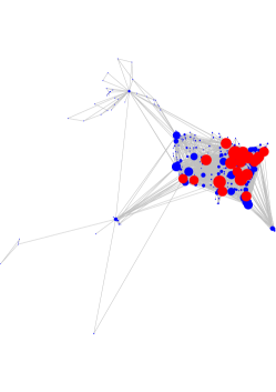
Figure 5.7: Snapshots of the melting process of the USAir97 network at three different values of $\beta$, namely at$1.5\cdot 10^{-7}$(a),$1.25\cdot 10^{-7}$(b),$1.0\cdot 10^{-7}$(c).

6 Conclusions and future outlook

The most important result of the current work is the proof of the existence of a universal melting transition in graphs and networks. This transition takes place when we consider a Lindemann-like model on graphs, which is based on a vibrational approach of nodes and edges. From a mathematical point of view the current method is based on the spectral properties of the adjacency matrix of the graph and the changes taking place on the exponential matrix function $\exp\left(\beta A\right)$ with the changes of $\beta$. In this way, regular-like graphs like square lattices are easier to melt than more irregular structures, such as spatial planar graphs. These differences resemble the known dissimilarities between crystalline and amorphous solids in their melting.

The analysis of a series of real-world networks has given us the possibility of exploring the global and local structural characteristics of networks which drives their melting. At the global topological level, we have shown here that the value $\beta_{c}$ at which the melting of a graph occurs depends mainly on the differences between the local and global degree heterogeneities existing in the graph. At the local one we have observed that the melting is triggered by the nodes having the higher eigenvector centrality in the network, particularly in those cases where the melting temperature is very close to zero.

The analysis of graph/networks melting as proposed here opens many new possibilities for the study of network robustness to external stresses. There are many mathematical and computational questions that remain open from the current study. They include, but are not limited, to the following ones: (i) A more exhaustive analysis of the topological (global and local) drivers of the graph melting; (ii) How certain specific network characteristics, e.g., clustering, modularity, degree assortativity, etc., influence the melting temperature and the melting process of artificial and real-world networks?; (iii) Is there a ranking of certain classes of graphs, e.g., trees, monocyclic graphs, etc., according to their melting? We hope the reader can help to answer some of these questions and generate new ones that clarify our understanding of network robustness to external stresses.

References

- [1] S. Alexander, Amorphous solids: their structure, lattice dynamics and elasticity, Physics reports, 296 (1998), pp. 65–236.
- [2] V. Alexiades, Mathematical modeling of melting and freezing processes, CRC Press, 1992.
- [3] R. Boese, H.-C. Weiss, and D. Bläser, The melting point alternation in the short-chain n-alkanes: single-crystal x-ray analyses of propane at 30 k and of n-butane to n-nonane at 90 k, Angewandte Chemie International Edition, 38 (1999), pp. 988–992.
- [4] R. W. Cahn, Melting and the surface, Nature, 323 (1986), pp. 668–669.
- [5] I. M. Campbell, R. A. James, E. S. Chen, and C. A. Shaw, Netcomm: a network analysis tool based on communicability, Bioinformatics, (2014), p. btu536.
- [6] I. M. Campbell, M. Rao, S. D. Arredondo, S. R. Lalani, Z. Xia, S.-H. L. Kang, W. Bi, A. M. Breman, J. L. Smith, C. A. Bacino, et al., Fusion of large-scale genomic knowledge and frequency data computationally prioritizes variants in epilepsy, PLoS Genet, 9 (2013), p. e1003797.
- [7] H. Chan and L. Akoglu, Optimizing network robustness by edge rewiring: a general framework, Data Mining and Knowledge Discovery, 30 (2016), pp. 1395–1425.
- [8] J. J. Crofts, D. J. Higham, R. Bosnell, S. Jbabdi, P. M. Matthews, T. Behrens, and H. Johansen-Berg, Network analysis detects changes in the contralesional hemisphere following stroke, Neuroimage, 54 (2011), pp. 161–169.
- [9] E. Estrada, The structure of complex networks: theory and applications, Oxford University Press, 2012.
- [10] , Graph and network theory, Mathematical Tools for Physicists, Wiley, (2013).
- [11] E. Estrada and N. Hatano, Statistical-mechanical approach to subgraph centrality in complex networks, Chemical Physics Letters, 439 (2007), pp. 247–251.
- [12] , Communicability in complex networks, Physical Review E, 77 (2008), p. 036111.
- [13] E. Estrada, N. Hatano, and M. Benzi, The physics of communicability in complex networks, Physics reports, 514 (2012), pp. 89–119.
- [14] E. Estrada and D. J. Higham, Network properties revealed through matrix functions, SIAM review, 52 (2010), pp. 696–714.
- [15] K. R. Gabriel and R. R. Sokal, A new statistical approach to geographic variation analysis, Systematic Biology, 18 (1969), pp. 259–278.
- [16] Y. Iturria-Medina, Anatomical brain networks on the prediction of abnormal brain states, Brain connectivity, 3 (2013), pp. 1–21.
- [17] Z. Jin, P. Gumbsch, K. Lu, and E. Ma, Melting mechanisms at the limit of superheating, Physical Review Letters, 87 (2001), p. 055703.
- [18] Y. Li, V. Jewells, M. Kim, Y. Chen, A. Moon, D. Armao, L. Troiani, S. Markovic-Plese, W. Lin, and D. Shen, Diffusion tensor imaging based network analysis detects alterations of neuroconnectivity in patients with clinically early relapsing-remitting multiple sclerosis, Human brain mapping, 34 (2013), pp. 3376–3391.
- [19] F. A. Lindemann, The calculation of molecular eigen-frequencies, Phys. Z.,(West Germany), 11 (1910), pp. 609–612.
- [20] X. Ma and L. Gao, Predicting protein complexes in protein interaction networks using a core-attachment algorithm based on graph communicability, Information Sciences, 189 (2012), pp. 233–254.
- [21] B. D. MacArthur, A. Sevilla, M. Lenz, F.-J. Müller, B. M. Schuldt, A. A. Schuppert, S. J. Ridden, P. S. Stumpf, M. Fidalgo, A. Maayan, et al., Nanog-dependent feedback loops regulate murine embryonic stem cell heterogeneity, Nature cell biology, 14 (2012), pp. 1139–1147.
- [22] M. Mancini, M. A. De Reus, L. Serra, M. Bozzali, M. P. Van Den Heuvel, M. Cercignani, and S. Conforto, Network attack simulations in alzheimer’s disease: The link between network tolerance and neurodegeneration, in Biomedical Imaging (ISBI), 2016 IEEE 13th International Symposium on, IEEE, 2016, pp. 237–240.
- [23] L. Mander, S. C. Dekker, M. Li, W. Mio, S. W. Punyasena, and T. M. Lenton, A morphometric analysis of vegetation patterns in dryland ecosystems, Open Science, 4 (2017), p. 160443.
- [24] L. Mander, M. Li, W. Mio, C. C. Fowlkes, and S. W. Punyasena, Classification of grass pollen through the quantitative analysis of surface ornamentation and texture, Proceedings of the Royal Society of London B: Biological Sciences, 280 (2013), p. 20131905.
- [25] M. E. Newman, The structure and function of complex networks, SIAM review, 45 (2003), pp. 167–256.
- [26] L. Papadopoulos, M. A. Porter, K. E. Daniels, and D. S. Bassett, Network analysis of particles and grains, arXiv preprint arXiv:1708.08080, (2017).
- [27] S. R. Phillpot, S. Yip, and D. Wolf, How do crystals melt?, Computers in physics, 3 (1989), pp. 20–31.
- [28] D. L. Powers, Graph partitioning by eigenvectors, Linear Algebra and its Applications, 101 (1988), pp. 121 – 133.
- [29] J. H. Smith, Some properties of the spectrum of a graph, Combinatorial Structures and their applications, (1970), pp. 403–406.
- [30] J. C. Urschel and L. T. Zikatanov, Spectral bisection of graphs and connectedness, Linear Algebra and its Applications, 449 (2014), pp. 1 – 16.
- [31] S. R. Vippagunta, H. G. Brittain, and D. J. Grant, Crystalline solids, Advanced drug delivery reviews, 48 (2001), pp. 3–26.
- [32] D. M. Walker and A. Tordesillas, Topological evolution in dense granular materials: a complex networks perspective, International Journal of Solids and Structures, 47 (2010), pp. 624–639.
- [33] Z. Wang, F. Wang, Y. Peng, and Y. Han, Direct observation of liquid nucleus growth in homogeneous melting of colloidal crystals, Nature communications, 6 (2015).