Exact Bremsstrahlung functions in ABJM theory

Abstract

In this paper we study the Bremsstrahlung functions for the $\frac{1}{6}$BPS and the $\frac{1}{2}$BPS Wilson lines in ABJM theory. First we use a superconformal defect approach to prove a conjectured relation between the Bremsstrahlung functions associated to the geometric ($B^{\varphi}_{1/6}$) and R-symmetry ($B^{\theta}_{1/6}$) deformations of the $\frac{1}{6}$BPS Wilson line. This result, non-trivially following from a defect supersymmetric Ward identity, provides an exact expression for $B^{\theta}_{1/6}$ based on a known result for $B^{\varphi}_{1/6}$. Subsequently, we explore the consequences of this relation for the $\frac{1}{2}$BPS Wilson line and, using the localization result for the multiply wound Wilson loop, we provide an exact closed form for the corresponding Bremsstrahlung function. Interestingly, for the comparison with integrability, this expression appears particularly natural in terms of the conjectured interpolating function $h(\lambda)$. During the derivation of these results we analyze the protected defect supermultiplets associated to the broken symmetries, including their two- and three-point correlators.

1 Introduction and results

Exact results for interacting quantum field theories are notoriously hard to achieve. Recent years, however, have seen spectacular developments in the computation of exact physical observables for conformal field theories with extended supersymmetry. These theories, despite their little phenomenological interest, constitute an important laboratory for testing our understanding of the finite coupling regime of quantum field theories.

The maximally supersymmetric theory in four dimensions, $\mathcal{N}=4$ Super Yang-Mills (SYM), is a celebrated example where supersymmetric localization Pestun:2016zxk as well as the discovery of an integrable structure Minahan:2002ve made such developments possible. While the former applies to a restricted class of protected observables (those that are annihilated by some supercharges), the latter proved very powerful for the computation of planar anomalous dimensions, inherently unprotected quantities. Therefore, despite the application of integrability has recently been extended to a wider range of observables, for some time it has been difficult to find a physical quantity accessible to both techniques. Luckily, the authors of Correa:2012at realized that the energy emitted by a moving particle, commonly known as Bremsstrahlung function, is a good candidate. On the one hand, it is suited for the integrability approach Correa:2012hh ; Drukker:2012de since it appears in the small angle expansion of the cusp anomalous dimension. On the other hand, interpreting the Wilson line as a superconformal defect Correa:2012at ; Cooke:2017qgm ; Giombi:2017cqn , the Bremsstrahlung function can be related to the first-order deformation of the circular Wilson loop expectation value Fiol:2012sg ; Correa:2012at , known exactly via localization Pestun:2009nn ; Erickson:2000af ; Drukker:2000rr ; Pestun:2007rz . The same match between integrability Gromov:2013qga ; Gromov:2015dfa and localization Bonini:2015fng happens for the generalized Bremsstrahlung function with $L$ units of R-charge.

Besides providing a highly non-trivial check of the result, computing the same quantity in two different ways allows to understand the precise identification of the parameters. Indeed, every integrability computation features a parameter $h$ whose relation with the ’t Hooft coupling $\lambda$ cannot be fixed by symmetry considerations. Whereas such relation turns out to be trivial for $\mathcal{N}=4$ SYM, this is not the case for its three-dimensional relative $\mathcal{N}=6$ super Chern-Simons theory with matter, known as ABJM theory Aharony:2008ug . In the latter case, a conjectured expression for $h(\lambda)$ Gromov:2014eha agrees with weak Gaiotto:2008cg ; Grignani:2008is ; Nishioka:2008gz ; Minahan:2009aq ; Minahan:2009wg ; Leoni:2010tb and strong McLoughlin:2008he ; Abbott:2010yb ; LopezArcos:2012gb ; Bianchi:2014ada coupling perturbative computations (see also Cavaglia:2016ide for the generalization to ABJ theory), but an exact derivation is still missing.

Similarities between ABJM and $\mathcal{N}=4$ SYM include the existence of a known string theory dual, the emergence of an integrable structure and the high degree of supersymmetry (although it is not maximal for ABJM). A crucial difference, instead, is the preserved supersymmetry of Wilson line operators. While the $\mathcal{N}=4$ SYM Maldacena-Wilson loop Maldacena:1998im preserves half of the supercharges (thus denoted as $\frac{1}{2}$BPS), its obvious ABJM generalization is annihilated by only $1/6$ of the supercharges ($\frac{1}{6}$BPS) Berenstein:2008dc ; Drukker:2008zx ; Chen:2008bp . A $\frac{1}{2}$BPS Wilson loop for ABJM, whose existence was expected as the dual to the fundamental string on $AdS_{4}\times\mathbb{CP}^{3}$, was built in Drukker:2009hy by introducing local couplings to the fermionic fields in the gauge superconnection.

The bosonic and fermionic Wilson loops are $\frac{1}{6}$BPS and $\frac{1}{2}$BPS respectively when their contour is maximally symmetric, i.e. a straight line or a circle. A smooth deformation of the contour, if combined with a suitable modification of the gauge connection, may still preserve a fraction of the original supersymmetry Cardinali:2012ru . On the other hand, when the Wilson line is deformed by a cusp, the supersymmetry is completely broken and the expectation value diverges. The coefficient of the divergent term, whose form can be analyzed in very general terms Polyakov:1980ca ; Korchemsky:1987wg , is called cusp anomalous dimension. Miming the four-dimensional case Drukker:1999zq ; Drukker:2011za , one can introduce a second deformation by an internal angle $\theta$ entering the local couplings with the bosonic and fermionic fields in the gauge superconnection. In this case the generalized cusp anomalous dimension $\Gamma_{\text{cusp}}(\varphi,\theta)$ would depend on both angles.

For ABJM, two different generalized cusps may be defined for the bosonic and fermionic Wilson lines Griguolo:2012iq ; Correa:2014aga . While for the former no residual BPS configuration could be found, for the latter the specific case $\varphi^{2}=\theta^{2}$ still preserves two supercharges, such that $\Gamma^{1/2}_{\text{cusp}}(\varphi,\pm\varphi)$ vanishes. This particular feature has interesting consequences for the small angle expansions of the two cusp anomalous dimensions. For the fermionic case one has

$$\Gamma^{1/2}_{\text{cusp}}(\varphi,\theta)\sim(\theta^{2}-\varphi^{2})B_{1/2}$$ (1)

which is the analogue of the four-dimensional case. This fact, supported by a three-loop computation, led to the conjecture of a relation between the Bremsstrahlung function and the first-order supersymmetric deformation of the circular $\frac{1}{2}$BPS Wilson loop (often denoted as latitude Wilson loop) Bianchi:2014laa ; Bianchi:2017svd . This relation was finally proven in Bianchi:2017ozk by relating $B_{1/2}$ to a particular combination of bosonic and fermionic two-point functions inserted on the Wilson line. In presence of a localization result for the latitude circular Wilson loop, this property would allow to compute $B_{1/2}$ exactly. Unfortunately no matrix model representation for the latitude Wilson loop is available and one has to rely on the fact that the bosonic and fermionic Wilson loops are cohomologically equivalent, i.e. their difference is exact with respect to a combination of the preserved supercharges. Elaborating on this and making some further assumptions, $B_{1/2}$ can be expressed in terms of the complex phase appearing in front of the Wilson loop expectation value, when computed with a contour splitting regularization Bianchi:2014laa ; Bianchi:2016yzj .

For the bosonic generalized cusp one can define two different Bremsstrahlung functions

$$\Gamma^{1/6}_{\text{cusp}}(\varphi,\theta)\sim\theta^{2}B^{\theta}_{1/6}-\varphi^{2}B^{\varphi}_{1/6}\,.$$ (2)

In this case, only $B^{\theta}_{1/6}$ can be related to the first order deformation of a circular Wilson loop Correa:2014aga . On the other hand, a completely different argument led to express $B^{\varphi}_{1/6}$ as the first order expansion of a $n$-wound Wilson loop for $n\to 1$ Lewkowycz:2013laa . Given the availability of localization results for the $n$-wound circular Wilson loop Kapustin:2009kz ; Marino:2009jd ; Drukker:2010nc ; Klemm:2012ii $B^{\varphi}_{1/6}$ is known exactly. Recently, the simple relation

$$B^{\varphi}_{1/6}=2B^{\theta}_{1/6}$$ (3)

was conjectured based on a finite $N$ four-loop computation Bianchi:2017afp ; Bianchi:2017ujp . Before this work, the apparent simplicity of (3) was not backed up by any (even speculative) field-theory argument and the lack of a genuine string computation of $B^{\theta}_{1/6}$ prevented a strong-coupling check, in contrast to the other Bremsstrahlung functions in ABJM.

In this paper we show that the identification (3) is a consequence of a supersymmetric Ward identity. The latter is derived in the framework of superconformal defects. The $\frac{1}{6}$BPS Wilson loop preserves a $su(1,1|1)\oplus su(2)\oplus su(2)$ subalgebra of the original $osp(6|4)$ ABJM symmetry algebra. The residual symmetry can be used to constrain defect correlation functions of local operators inserted along the Wilson line. Such insertions are organized in irreducible representations of the preserved subalgebra: long multiplets, whose scaling dimension is not protected, and short multiplets which are annihilated by one of the two preserved supercharges and whose dimension is fixed by algebraic arguments. Among the latter, we are particularly interested in those associated to the broken symmetries. Whenever a defect breaks a symmetry of the original theory the conservation law for the associated currents should be supplemented by some defect degrees of freedom. This relation with the previously conserved currents guarantees that these defect excitations are protected. A well studied example is the displacement operator which compensates for the non-conservation of the stress tensor and accounts for the breaking of translation invariance Billo:2016cpy . For supersymmetric theories we know that the stress tensor belongs to the same supermultiplet of the supersymmetry and R-symmetry currents Cordova:2016emh . For the defect setup we will clarify, using some algebraic arguments and showing explicit expressions, that the displacement operator is the top component (as should be expected Liendo:2016ymz ) of a supermultiplet containing also a fermionic operator associated to some broken supercharges. The defect excitations associated to the rest of the broken supercharges together with the R-symmetry ones form a different supermultiplet, which we denote as $R$-multiplet.

Focusing on these two supermultiplets we explore the constraints of the residual symmetries on two- and three-point functions. This task is eased by the observation that the preserved superalgebra coincides with the chiral part or the $\mathcal{N}=2$ superconformal algebra in two dimensions (of course only the global part, not the infinite dimensional super-Virasoro extension). This allows to exploit the results of Blumenhagen:1992sa ; DiVecchia:1985ief ; Mussardo:1988av for correlation functions in superspace. The outcome of this analysis is that two-point functions of operators belonging to the displacement and the R-multiplet are completely fixed by superconformal symmetry up to an overall factor, their Zamolodchikov norm. Interestingly, the Zamolodchikov norm of the displacement operator is related to the Bremsstrahlung function $B^{\varphi}_{1/6}$ Correa:2012at , while that of the R-multiplet is proportional to $B^{\theta}_{1/6}$ Correa:2014aga . Therefore the relation (3) establishes a connection between the Zamolodchikov norms of the two supermultiplets. We show that this connection can be derived through an unconventional Ward identity which uses the action of a supercharge that is not preserved by the defect. Such Ward identity, as it usually happens for defect field theories, mixes two- and three-point functions, but in our case we will be able to show that the symmetry is large enough to set to zero all the involved three-point functions, thus allowing to prove (3).

After this derivation we explore the consequences of our result. First of all we point out how equation (3) leads to a useful ansatz for the relation between the winding number $n$ and the deformation parameter $\nu$, characterizing the deformation of the maximal circular Wilson loop. We then extend this prescription to a relation between winding and framing and this allows to rederive the exact form for $B_{1/2}$ conjectured in Bianchi:2014laa as well as a relation between $B_{1/2}$ and $B_{1/6}^{\varphi}$. We conclude our work by expressing $B_{1/2}$ in a closed form. This may result useful from the point of view of integrability, since, if we take for granted the conjecture of Gromov:2014eha for $h(\lambda)$, our expression involves elliptic functions whose argument is naturally expressed in terms of $h$ rather than $\lambda$.

This paper is organized as follows. In section 2 we review the properties of bosonic and fermionic supersymmetric Wilson loops in ABJM, in particular we focus on the cusped Wilson loops and the related cusp anomalies and Bremsstrahlung functions. We also introduce some background for the study of Wilson line excitations as a defect one-dimensional superconformal field theory. In section 3 we study this field theory and the structure of their protected supermultiplets under the symmetry preserved by the bosonic line. In section 4 we introduce the relevant two- and three-point functions in both the defect theory and the related superspace. Exploiting some Ward identities involving conserved and non-conserved supercharges, we relate the Zamolodchikov norms of certain two-point functions to compute $B^{\theta}_{1/6}$ exactly. In section 5 we establish a relation between all the Bremsstrahlung functions via a unique function. The main result of section 6 is the exact closed form of $B_{1/2}$ in terms of the conjectured interpolating function $h(\lambda)$. Few appendices follow, which contain conventions and some details of the supermultiplets and the supersymmetry algebra.

2 BPS Wilson loops and the Bremsstrahlung functions in ABJM

The $\mathcal{N}=6$ Chern-Simons-matter theory, known as ABJM Aharony:2008ug ; Bandres:2008ry , is a three-dimensional superconformal field theory with $U(N)_{k}\times U(N)_{-k}$ gauge group, with $k$ being the integer Chern-Simons level. Its global symmetry is $OSp(6|4)$: the bosonic subsector of the supergroup contains the R-symmetry group $SO(6)\sim SU(4)$ and the Euclidean conformal group in three-dimensions $Sp(4)\sim SO(1,4)$, the fermionic subsector generates the $\mathcal{N}=6$ supersymmetries.

The theory has the following field content: two gauge fields ${(A_{\mu})_{i}}^{j}$ and ${(\hat{A}_{\mu})_{\hat{i}}}^{\hat{j}}$, belonging respectively to the adjoint of $U(N)_{k}$ and $U(N)_{-k}$, four complex scalars ${(C_{I})_{i}}^{\hat{j}}$ (or ${(\bar{C}^{I})_{\hat{i}}}^{j}$) as well as four complex fermions ${(\bar{\psi}^{I})_{i}}^{\hat{j}}$ (or ${(\psi_{I})_{\hat{i}}}^{j}$) belonging to the bifundamental (antibifundamental) of the gauge group $U(N)_{k}\times U(N)_{-k}$.

In this paper we are mostly interested in supersymmetric Wilson loops, a rich class of BPS observables that, in principle, can be known exactly. We start by reviewing the definition and properties of the bosonic and fermionic Wilson loop operators. We focus on a particular choice for the contour (cusped Wilson line) in order to define the cusp anomalous dimensions and the Bremsstrahlung functions summarizing the state of the art in the literature.

2.1 The bosonic Wilson loop

The bosonic Wilson loop Berenstein:2008dc ; Drukker:2008zx ; Chen:2008bp ; Rey:2008bh is a natural generalization of the four-dimensional Wilson-Maldacena loop Maldacena:1998im and it is defined as follows

$$\mathcal{W}_{B}[\mathcal{C}]=\frac{1}{N}\textup{Tr}\left[\mathcal{P}\exp\left({-i\int_{\mathcal{C}}d\tau~{}\mathcal{L}_{B}(\tau)}\right)\right]\quad\text{with}\quad\mathcal{L}_{B}=A_{\mu}\dot{x}^{\mu}-\frac{2\pi i}{k}|\dot{x}|\,M_{J}^{\ \ I}C_{I}\bar{C}^{J}\,,$$ (4)

where $\mathcal{C}$ is the path along which the loop is supported parametrized by $x(\tau)$, $\mathcal{P}$ is the path-ordering operator and the trace Tr is taken in the fundamental representation of $U(N)_{k}$. One can also define an analogous Wilson loop operator $\hat{\mathcal{W}}_{B}[\mathcal{C}]$ belonging to the fundamental representation of $U(N)_{-k}$, where the connection $\hat{\mathcal{L}}_{B}$ contains $\hat{A}_{\mu}$ instead of $A_{\mu}$ and $\hat{M}_{J}^{\ \ I}\bar{C}^{J}C_{I}$ instead of $M_{J}^{\ \ I}C_{I}\bar{C}^{J}$. The scalar coupling $M_{J}^{\ \ I}$ and $\hat{M}_{J}^{\ \ I}$ are in general matrices with arbitrary entries. They can be constrained by supersymmetry imposing the standard vanishing condition

$$\delta_{\text{susy}}\mathcal{L}_{B}=0\,.$$ (5)

and using the supersymmetry transformations in (189). The choice of which supercharges are preserved by the Wilson loop (4) fixes both the scalar couplings and the contour parametrization.

In order to study the most general class of supersymmetric Wilson loops, it is convenient to consider operators lying on curves on the sphere $S^{2}$. These loops can be mapped to their equivalent operators in flat space through a conformal map that maintains the number of preserved supercharges. In this setting, an arbitrary curve on $S^{2}$ preserves 1/24 of the total number of supersymmetries and the equator corresponds to the maximally supersymmetric operator, namely $\frac{1}{6}$BPS. It is also possible to consider an operator with an intermediate number of preserved supersymmetries. This operator is called $\frac{1}{12}$BPS bosonic latitude Wilson loop and it can be written as a two-parameter deformation of the $\frac{1}{6}$BPS Wilson loop. These parameters combine in a single quantity that the Wilson loop depends on Bianchi:2014laa

$$\nu=\sin{2\alpha}\cos\theta_{0}\qquad\text{with}\quad-\pi/2\leq\theta_{0}\leq\pi/2\;\;\text{and}\;\;0\leq\alpha\leq\pi/4\,.$$ (6)

The only relevant deformation appears in the scalar couplings of (4) which can be written in terms of $\nu$ as follows

$${M_{J}}^{I}(\nu)={\hat{M}_{J}}{}^{I}(\nu)=\begin{pmatrix}-\nu&0&e^{-i\tau}\sqrt{1-\nu^{2}}&0\\ 0&-1&0&0\\ e^{i\tau}\sqrt{1-\nu^{2}}&0&\nu&0\\ 0&0&0&1\end{pmatrix}\,.$$ (7)

The expectation value of the latitude Wilson loop depends only on $\nu$, so we refer to the operator as $\mathcal{W}_{B}(\nu)$.

In the limit $\nu\rightarrow 1$ we recover the $\frac{1}{6}$BPS Wilson loop on the maximal circle of $S^{2}$. Through a particular conformal mapping, we can project this loop on the plane obtaining the $\frac{1}{6}$BPS infinite straight Wilson line with the contour parametrized by

$$x^{\mu}=\{\tau,0,0\}\qquad\text{with}\quad-\infty<\tau<\infty$$ (8)

and the scalar couplings given by

$${M_{J}}^{I}(1)={\hat{M}_{J}}{}^{I}(1)=\begin{pmatrix}-1&0&0&0\\ 0&-1&0&0\\ 0&0&1&0\\ 0&0&0&1\end{pmatrix}\,.$$ (9)

This operator preserves a $su(1,1|1)\oplus su(2)\oplus su(2)$ subalgebra of $osp(6|4)$ (see appendix C for the details). In the following we refer to it as $\mathcal{W}_{1/6}$. We summarize the relations between the supersymmetric Wilson loops above as follows

$$\underset{\text{$\frac{1}{12}$BPS latitude on $S^{2}$}}{\mathcal{W}_{B}(\nu)}\xrightarrow{\nu\rightarrow 1}\underset{\text{$\frac{1}{6}$BPS circle on $S^{2}$}}{\mathcal{W}_{B}(1)}\xrightarrow{\text{conf. map}}\underset{\text{$\frac{1}{6}$BPS line in $\mathbb{R}^{3}$}}{\mathcal{W}_{1/6}}\,.$$ (10)

A string configuration for the bosonic Wilson loop is still elusive. Since the fundamental string ending along the Wilson loop contour on the boundary of $AdS_{4}$ and localized in $\mathbb{CP}^{3}$ preserves more supercharges, a smearing of the string over a $\mathbb{CP}^{1}$ is expected to break the supersymmetry in order to match with the gauge theory observable Drukker:2008zx ; Rey:2008bh .

2.2 The fermionic Wilson loop

In order to match the number of supercharges preserved by the fundamental string in $AdS_{4}\times\mathbb{CP}^{3}$, on the field theory side one needs to consider the holonomy of a $U(N|N)$ superconnection Drukker:2009hy ; Lee:2010hk . This operator with an arbitrary contour was given in Cardinali:2012ru where it was expressed as

$$\mathcal{W}_{F}[\mathcal{C}]=\frac{1}{\textup{Str}\,\mathcal{T}}\,\textup{Str}\left[\mathcal{P}\exp\left(-i\int_{\mathcal{C}}d\tau\,\mathcal{L}_{F}(\tau)\right)\mathcal{T}\right]$$ (11)

with a superconnection $\mathcal{L}_{F}(\tau)$

$$\mathcal{L}_{F}=\begin{pmatrix}A_{\mu}\dot{x}^{\mu}-\frac{2\pi i}{k}|\dot{x}|{\mathcal{M}_{J}}^{I}C_{I}\bar{C}^{J}&-i\sqrt{\frac{2\pi}{k}}|\dot{x}|\eta_{I}\bar{\psi}^{I}\\ -i\sqrt{\frac{2\pi}{k}}|\dot{x}|\psi_{I}\bar{\eta}^{I}&\hat{A}_{\mu}\dot{x}^{\mu}-\frac{2\pi i}{k}|\dot{x}|{\hat{\mathcal{M}}_{J}}^{I}\bar{C}^{J}C_{I}\end{pmatrix}\,.$$ (12)

Here Str stands for the usual supertrace taken in the fundamental representation and the quantities ${\mathcal{M}_{J}}^{I}(\tau)$, ${\hat{\mathcal{M}}_{J}}^{I}(\tau)$, $\eta_{I}(\tau)$ and $\bar{\eta}^{I}(\tau)$ are local couplings. As for the bosonic case, one can determine the form of the couplings in terms of the contour $x^{\mu}(\tau)$ by the requirement of preserving some of the supercharges. In this case the standard vanishing condition $\delta_{\text{susy}}\mathcal{L}_{F}=0$ is too strong and it can be replaced by the weaker requirement Drukker:2009hy ; Lee:2010hk ; Cardinali:2012ru

$$\delta_{\text{susy}}\mathcal{L}_{F}=\mathcal{D}_{\tau}\mathcal{G}\equiv\partial_{\tau}\mathcal{G}+i[\mathcal{L},\mathcal{G}]\,,$$ (13)

where $\mathcal{G}$ is a $u(N|N)$ supermatrix. The twist supermatrix $\mathcal{T}$ in (11) is needed for the operator to be gauge invariant.

We are interested in some particular configurations of the fermionic Wilson loop: the latitude and maximal circle on $S^{2}$ and the infinite straight line in $\mathbb{R}^{3}$. Using the relation (13) and the supersymmetry transformations (189), it turns out that the fermionic maximal circle is $\frac{1}{2}$BPS, matching the supersymmetry preserved by the fundamental string in $AdS_{4}\times\mathbb{CP}^{3}$. As in the previous case the latitude Wilson loop can be seen as a two-parameter deformation of the maximally supersymmetric operator on the equator. Those parameters can be rearranged again in the single quantity (6) and the Wilson loop expectation value depends only on it. We then refer to the 1/6 fermionic latitude as $\mathcal{W}_{F}(\nu)$. The operator on the maximal circle can be recovered in the limit $\nu\rightarrow 1$. Using the stereographic conformal projection, this operator is mapped in the $\frac{1}{2}$BPS fermionic Wilson line lying on the contour parametrized by (8). This operator preserves a $su(1,1|3)$ subalgebra of $osp(6|4)$ (see Bianchi:2017ozk for the details). In the following we refer to it as $\mathcal{W}_{1/2}$. All the details about the scalar and fermionic couplings for any of the previous configurations can be found in Drukker:2009hy ; Cardinali:2012ru . We repeat below the relation among fermionic Wilson loops for clarity:

$$\underset{\text{$\frac{1}{6}$BPS latitude on $S^{2}$}}{\mathcal{W}_{F}(\nu)}\xrightarrow{\nu\rightarrow 1}\underset{\text{$\frac{1}{2}$BPS circle on $S^{2}$}}{\mathcal{W}_{F}(1)}\xrightarrow{\text{conf. map}}\underset{\text{$\frac{1}{2}$BPS line in $\mathbb{R}^{3}$}}{\mathcal{W}_{1/2}}\,.$$ (14)

2.3 The generalized cusp and the Bremsstrahlung functions in ABJM

Let us start consider a bosonic or fermionic Wilson line with contours $C_{1}$ and $C_{2}$ in $\mathbb{R}^{3}$ intersecting in the origin and forming the curve $C=C_{1}\cup C_{2}$ (see Figure 1) with parametrization

$$C:\qquad x^{\mu}=\{\tau\cos\frac{\varphi}{2},|\tau|\sin\frac{\varphi}{2},0\}\qquad\text{with}\quad-L\leq\tau\leq L\,,$$ (15)

where $L$ is an IR cut-off. In general one can introduce an extra parameter $\theta$ that corresponds to the angular separation of the Wilson lines on $C_{1}$ and $C_{2}$ in the R-symmetry space.

Figure 1: The planar Euclidean cusp with angular opening $\pi-\varphi$ between the Wilson lines.

This deformation affect the scalar and fermionic couplings in (4) and (11). Considering the factorized form of the fermionic coupling $\eta_{I}^{\alpha}=n_{I}\eta^{\alpha}$ (the same for the complex conjugate) and that $\hat{M}=M$ and $\hat{\mathcal{M}}=\mathcal{M}$, the contractions of the couplings are defined as follows

$$M_{i}\cdot M_{j}=\mathcal{M}_{i}\cdot\mathcal{M}_{j}=\begin{cases}4\cos^{2}\frac{\theta}{2}&\quad i\neq j\\ 4&\quad i=j\end{cases}\qquad n_{i}\cdot\bar{n}_{j}=\begin{cases}2i\cos\frac{\theta}{2}&\quad i\neq j\\ 2i&\quad i=j\end{cases}$$ (16)

where $i,j=1,2$ and $\{M_{1},\mathcal{M}_{1},n_{1},\bar{n}_{1}\}\in C_{1}$ and $\{M_{2},\mathcal{M}_{2},n_{2},\bar{n}_{2}\}\in C_{2}$. The twist supermatrix $\mathcal{T}$ in (11) in this case is

$$\mathcal{T}=\begin{pmatrix}\mathbb{1}_{N}&0\\ 0&-\mathbb{1}_{N}\end{pmatrix}$$ (17)

and the supertrace becomes the usual trace in the fundamental representation and the normalization coefficient $\textup{Str}\,\mathcal{T}=2N$. This configuration is called generalized cusp.

Unlike the infinite straight lines, the bosonic and fermionic generalized cusped Wilson lines do not preserve any of the supersymmetries and develop logarithmically divergent, which lead in turn to the definition of the associated anomalous dimensions as

$$\begin{split}&\log\braket{\mathcal{W}_{B}[C]}\sim-\Gamma_{\text{cusp}}^{1/6}(\theta,\varphi)\log\frac{L}{\epsilon}+\mbox{finite}\\ \ &\log\braket{\mathcal{W}_{F}[C]}\sim-\Gamma_{\text{cusp}}^{1/2}(\theta,\varphi)\log\frac{L}{\epsilon}+\mbox{finite}\end{split}$$ (18)

where $C$ is the cusp contour (15), $L$ and $\epsilon$ are an IR and UV regulator respectively. The coefficients of the logarithms $\Gamma_{\text{cusp}}^{1/6}$ and $\Gamma_{\text{cusp}}^{1/2}$ are the cusp anomalous dimensions of the bosonic and fermionic cusped Wilson lines respectively. They are two important physical observables that control the IR divergences of scattering amplitudes of massive colored particles, besides the important properties outlined in the introduction. Furthermore, setting $\theta=0$ and performing the analytic continuation $\varphi\rightarrow i\infty$, one finds the light-like cusp anomalous dimension, whose value is computed exactly via integrability Beisert:2006ez ; Gromov:2008qe .

Over the last years, $\Gamma_{\text{cusp}}^{1/6}$ was studied at weak coupling in Griguolo:2012iq (for the strong coupling see the final comment of section 2.1). Also $\Gamma_{\text{cusp}}^{1/2}$ was extensively studied at both weak and strong coupling. Its value was computed at two loops via perturbation theory Griguolo:2012iq and exactly in the double scaling limit where only ladder diagrams contribute ($\lambda\rightarrow 0$, $i\theta\rightarrow\infty$ and $\lambda e^{i\theta/2}=\text{const}$) Bonini:2016fnc . The case $\varphi=0$ was explored at three loops using the HQET formalism in Bianchi:2017svd ; Preti:2017fjb . On the string theory side $\Gamma_{\text{cusp}}^{1/2}$ is known at next to leading order from Forini:2012bb ; Correa:2014aga .

As mentioned in the introduction, see (1) and (2), the small angle limit of the cusp anomalous dimension gives the Bremsstrahlung functions. The exact computation of the Bremsstrahlung functions in ABJM is an arduous task for which a complete proof is still elusive. Nevertheless, there exist some conjectured relations that connect each Bremsstrahlung function to the expectation value of the multiply-wound circular Wilson loop with bosonic couplings

$$\mathcal{W}^{n}_{B}(1)=\frac{1}{N}\textup{Tr}\left[\mathcal{P}\exp\left({-i\oint_{0}^{2\pi n}d\tau~{}\mathcal{L}_{B}(\tau)}\right)\right]$$ (19)

where the connection $\mathcal{L}_{B}(\tau)$ is defined in (4). The new parameter $n$ specifies the number of times that the loop, spanned by $\tau$, wraps the circular contour. This operator localizes on a matrix model Kapustin:2009kz that was solved in detail Marino:2009jd ; Drukker:2010nc ; Klemm:2012ii . The perturbative expansion of this exact result produces predictions for the Bremsstrahlung functions that match the direct computations of the generalized cusps with $\frac{1}{2}$BPS and $\frac{1}{6}$BPS rays at both weak and strong coupling.

A formula for the Bremsstrahlung function $B_{1/2}$, defined in (1) as the small angle limit of the cusp with $\frac{1}{2}$BPS rays, was proposed in Bianchi:2014laa as the derivative of the fermionic Wilson loop evaluated on a latitude on $S^{2}$ with respect to the deformation parameter $\nu$

$$B_{1/2}=\frac{1}{4\pi^{2}}\Big{.}\partial_{\nu}\log\langle\mathcal{W}_{F}(\nu)\rangle\Big{|}_{\nu=1}\,.$$ (20)

The relation was modelled upon an analogous result in $\mathcal{N}=4$ SYM Correa:2012at and it was later proven by applying superconformal defect constraints on the $\frac{1}{2}$BPS Wilson line insertions Bianchi:2017ozk . The relation with the multiply-wound Wilson loop on a circle articulates in a few steps that are reviewed in section 5.

The prediction for the Bremsstrahlung function $B^{\varphi}_{1/6}$ associated to the geometric cusp formed with $\frac{1}{6}$BPS rays was formulated in Lewkowycz:2013laa

$$B^{\varphi}_{1/6}=\frac{1}{4\pi^{2}}\Big{.}\partial_{n}\log|\langle\mathcal{W}^{n}_{B}\rangle|\Big{|}_{n=1}\,,$$ (21)

where the expectation value is computed at framing 1 (see section 5.1). This result stems from a chain of relations between different observables which leads to the $\frac{1}{6}$BPS Wilson loop that winds around the circle $n$ times, although a few steps are not proven with full rigour. It is not necessary to review them in this paper and one can refer to Bianchi:2014laa for a concise summary. However, it is useful to remember that (21) passed a non-trivial test for the first few weak-coupling perturbative orders Griguolo:2012iq ; Bianchi:2014laa and it is consistent with string-theory calculations at leading and subleading order Correa:2014aga ; Aguilera-Damia:2014bqa .

In this paper we focus on the Bremsstrahlung function $B^{\theta}_{1/6}$ that corresponds to a cusp distortion in R-symmetry space along a $\frac{1}{6}$BPS straight line. A relation with the bosonic loop 

$$B^{\theta}_{1/6}=\frac{1}{4\pi^{2}}\Big{.}\partial_{\nu}\log|\langle\mathcal{W}_{B}(\nu)\rangle|\Big{|}_{\nu=1}$$ (22)

was derived by means of a similar proof in $\mathcal{N}=4$ SYM Correa:2012at which involves two-point function of scalar operators inserted along the circular Wilson loop Correa:2014aga . The notable complication with respect to the four-dimensional case is again the fact that the right-hand side in (22) is only known perturbatively, thus preventing the derivation of an all-loop expression for $B^{\theta}_{1/6}$. A few perturbative orders were checked from the bosonic Wilson loop at two loops Bianchi:2014laa . At the moment a strong-coupling check is hindered by the lack of the string configuration dual to the latitude Wilson loop with bosonic couplings, despite some attempts of “string smearing” Correa:2014aga . There exists a proposed relation for $B^{\theta}_{1/6}$ given in (3) that relates it to the putative (21).

2.4 Wilson lines as superconformal defects

In this paper we are interested in computing the expectation value of a Wilson loop with local operators inserted along the contour. Given some local operators $\mathcal{O}_{i}(\tau_{i})$, one can define the gauge invariant Wilson line with insertions

$$\mathcal{W}[\mathcal{O}_{1}(\tau_{1})\mathcal{O}_{2}(\tau_{2})\,...\,\mathcal{O}_{n}(\tau_{n})]\equiv\textup{Tr}\mathcal{P}\left[\mathcal{W}_{\tau_{i},\tau_{1}}\mathcal{O}_{1}(\tau_{1})\mathcal{W}_{\tau_{1},\tau_{2}}\mathcal{O}_{2}(\tau_{2})\,...\,\mathcal{O}_{n}(\tau_{n})\mathcal{W}_{\tau_{n},\tau_{f}}\right]$$ (23)

where $\mathcal{W}_{\tau_{a},\tau_{b}}$ is a fermionic or bosonic Wilson line that starts at position $x(\tau_{a})$ and ends at position $x(\tau_{b})$. Also, $\tau_{i}=\tau_{f}$ for a closed loop and $\tau_{i}=-\infty$ and $\tau_{f}=\infty$ for an infinite straight line. Since the local operators $\mathcal{O}_{i}(\tau_{i})$ are inserted between (untraced) Wilson lines, they have to transform in the same representation of the gauge group. In this paper we are only interested in operator insertions on the bosonic Wilson loop $\mathcal{W}_{B}$, whose connection transforms in the adjoint of $U(N)_{k}$, so we look at operators belonging to the same representation. The vacuum expectation value of (23) can be interpreted as a $n$-point correlation function of local operators where the vacuum is the supersymmetric Wilson loop $\mathcal{W}$:

$$\langle\mathcal{O}_{1}(\tau_{1})\mathcal{O}_{2}(\tau_{2})\,...\,\mathcal{O}_{n}(\tau_{n})\rangle_{\mathcal{W}}\equiv\frac{\langle\mathcal{W}[\mathcal{O}_{1}(\tau_{1})\mathcal{O}_{2}(\tau_{2})\,...\,\mathcal{O}_{n}(\tau_{n})]\rangle}{\langle\mathcal{W}\rangle}\,.$$ (24)

This is nothing but a correlation function in a one-dimensional defect. When the residual symmetry preserved by the corresponding Wilson loop includes the conformal group, the correlation functions defined by (24) satisfy all the axioms of a one-dimensional CFT. For instance, if the contour is a straight line, the fermionic and bosonic defects preserve $SU(1,1|3)$ Bianchi:2017ozk and $SU(1,1|1)$ (see section 3) superconformal groups respectively. In this setting, operator insertions can be organized according to the representations of the preserved supergroup. Particular care, however, must be devoted to the conformal descendants. Indeed for Wilson loop correlators one has the defining property

$$\langle\,...\,\mathcal{D}_{\tau}\mathcal{O}(\tau)\,...\,\rangle_{\mathcal{W}}=\partial_{\tau}\langle\,...\,\mathcal{O}(\tau)\,...\,\rangle_{\mathcal{W}}$$ (25)

where $\mathcal{D}_{\tau}$ is the covariant derivative taken with respect to the total connection of the loop $\mathcal{W}$. For the case of interest here, we consider the following definition

$$\mathcal{D}_{\tau}\mathcal{O}(\tau)\equiv\partial_{\tau}+i[\mathcal{L}_{B},\mathcal{O}(\tau)]\,.$$ (26)

The implication of equation (25) is that, in building the representations of the superconformal algebra for inserted operators, the covariant derivative $\mathcal{D}_{\tau}$ plays the role of the ordinary derivative in standard CFT, i.e. the generator of translations along the line.

In the following we will need to consider the action of a generic infinitesimal variation on a Wilson line. This translates into operator insertions as

$$\delta(\log\mathcal{W}[\mathcal{C}])=-i\int_{\mathcal{C}}d\tau\,\langle\delta\mathcal{L}(\tau)\rangle_{\mathcal{W}}$$ (27)

where $\mathcal{L}$ is the bosonic or fermionic Wilson loop connection depending on which operator $\mathcal{W}$ we are considering. The operator $\delta$ corresponds to any infinitesimal transformation. In particular, if it represents a supersymmetry transformation, it can be written as $\delta=\epsilon\mathcal{Q}$ where $\mathcal{Q}$ is a supercharge and $\epsilon$ a Grassmann infinitesimal parameter. In this paper we are interested in infinitesimal deformations of two-point functions on the defect that can be written as

$$\begin{split}\delta\langle\mathcal{O}_{1}(\tau_{1})\mathcal{O}_{2}(\tau_{2})\rangle_{\mathcal{W}}\!=&\langle\delta\mathcal{O}_{1}(\tau_{1})\mathcal{O}_{2}(\tau_{2})\rangle_{\mathcal{W}}\!+\langle\mathcal{O}_{1}(\tau_{1})\delta\mathcal{O}_{2}(\tau_{2})\rangle_{\mathcal{W}}\!-\!i\!\!\int_{\tau_{i}}^{\tau_{1}}\!\!\!d\tau\langle\delta\mathcal{L}(\tau)\mathcal{O}_{1}(\tau_{1})\mathcal{O}_{2}(\tau_{2})\rangle_{\mathcal{W}}\!\\ &-i\int_{\tau_{1}}^{\tau_{2}}d\tau\,\langle\mathcal{O}_{1}(\tau_{1})\delta\mathcal{L}(\tau)\mathcal{O}_{2}(\tau_{2})\rangle_{\mathcal{W}}-i\int_{\tau_{2}}^{\tau_{f}}d\tau\,\langle\mathcal{O}_{1}(\tau_{1})\mathcal{O}_{2}(\tau_{2})\delta\mathcal{L}(\tau)\rangle_{\mathcal{W}}\,.\end{split}$$ (28)

This transformation generates defect three-point functions when it is applied to the Wilson loop as in (27). Notice that, if the deformation is a supersymmetric transformation, the relative signs in the right-hand side of (28) can change depending on the position of the Grassmann infinitesimal parameter. Also, if the vacuum of the original theory is invariant under the variation $\delta$, one can use equation (28) to derive Ward identities as we do in section (4.3).

3 Symmetry considerations

The $\frac{1}{6}$BPS Wilson line defined in (4), when the contour is an infinite straight line or a circle, preserves a $su(1,1|1)\oplus su(2)\oplus su(2)$ subalgebra of the full $osp(6|4)$ ABJM superalgebra. Commutation relations of such subalgebra are given in appendix C, where we also review its representation theory. Here we consider the fundamental fields of the theory and how they organize in representations of the preserved symmetries. The $SU(4)$ R-symmetry group is broken down to $SU(2)\times SU(2)\times U(1)$. The preserved supercharges $Q^{12}_{+}\equiv Q$ and $Q^{34}_{-}\equiv\bar{Q}$ are neutral under the two $SU(2)$ factors and oppositely charged under $U(1)$ (this $U(1)$ is a bosonic subalgebra of $SU(1,1|1)$ as detailed in appendix C). Therefore the action of the supercharges on a highest weight state does not affect the $SU(2)$ charges, but only its $U(1)$ charge. Matter fields can be split according to the new symmetry. We use an index $a$ for the fundamental representation of the first $SU(2)$ and an index $\dot{a}$ for the second one. For the bosons we have

$$C_{I}=(C_{a} ,C_{\dot{a}}) \bar{C}^{I}=(\bar{C}^{a} ,\bar{C}^{\dot{a}})$$ (29)

$$U(1) (-\tfrac{1}{2} ,\phantom{-}\tfrac{1}{2}) (\phantom{-}\tfrac{1}{2} ,-\tfrac{1}{2})$$ charge

whereas for the fermions

$$\psi^{+}_{I}=(\psi^{+}_{a} ,\psi^{+}_{\dot{a}}) \psi^{-}_{I}=(\psi^{-}_{a} ,\psi^{-}_{\dot{a}}) \bar{\psi}_{+}^{I}=(\bar{\psi}_{+}^{a} ,\bar{\psi}_{+}^{\dot{a}}) \bar{\psi}_{-}^{I}=(\bar{\psi}_{-}^{a} ,\bar{\psi}_{-}^{\dot{a}})$$ (30)

$$U(1) (\phantom{-}0 ,\phantom{-}1) (-1 ,\phantom{-}0) (\phantom{-}0 ,-1) (\phantom{-}1 ,\phantom{-}0)$$ charge

In the present paper we are interested in operator insertions on the Wilson lines. Those insertions are organized in representations of the preserved superalgebra and we will be concerned with operators which belong to short multiplets. In appendix C we show that the $su(1,1|1)$ superalgebra allows for two possible shortening conditions, leading to the $\frac{1}{2}$BPS multiplets $\mathcal{B}_{j}$, annihilated by Q, and $\bar{\mathcal{B}}_{j}$, annihilated by $\bar{Q}$. Looking at the supersymmetry transformations in appendix D.1 we immediately find the first examples of short multiplets. Indeed the operators $C_{a}$ and $\bar{C}_{\dot{a}}$ are annihilated by $\bar{Q}$ and they are superprimaries of a $\bar{\mathcal{B}}_{-\frac{1}{2}}$, while the operators $\bar{C}^{a}$ and $C_{\dot{a}}$ are superprimaries of $\mathcal{B}_{\frac{1}{2}}$.

Notice however that these operators change in the bifundamental representation of the gauge group $U(N)_{k}\times U(N)_{-k}$ and in order to build insertions of the kind (24) we would need to use both $\mathcal{W}_{B}$ and $\hat{\mathcal{W}}_{B}$. We now look for short multiplets which are singlet under the second $U(N)$ factor, allowing us to use only the Wilson line $\mathcal{W}_{B}$.

3.1 Broken currents and defect operators

The straight Wilson line breaks some of the original symmetries and, as a consequence, some of the currents are no longer conserved. A prototypical example is that of spacetime translation, for which the stress tensor conservation is broken to

$$\partial_{\mu}T^{\mu i}=\delta^{2}(x^{j})\mathbb{D}^{i}(\tau)$$ (31)

where $i,j=2,3$ are directions orthogonal to the line, the delta function localizes the r.h.s. on the defect profile (a straight line along the direction 1 in this case) and $\mathbb{D}^{i}$ is the displacement operator. Of course equation (31) is written in a loose notation and it must be interpreted as a Ward identity when both sides are inserted inside a correlation function with other operators. In the following, we will use complex coordinates in the orthogonal directions and work with the complex combinations $\mathbb{D}=\mathbb{D}_{2}-i\mathbb{D}_{3}$ and $\bar{\mathbb{D}}=\mathbb{D}_{2}+i\mathbb{D}_{3}$. The broken momentum generators are also organized as $\mathfrak{P}\equiv P_{2}-iP_{3}$ and $\bar{\mathfrak{P}}\equiv P_{2}+iP_{3}$. The name displacement operator can be understood by looking at the integrated version of the Ward identity (31), which can be schematically written as

$$\braket{X}_{\delta_{\mathfrak{P}}W}=-\int d\tau\braket{\mathbb{D}(\tau)X}_{\mathcal{W}}\epsilon+\mathcal{O}(\epsilon^{2})$$ (32)

where $X$ is an arbitrary set of local operators and the notation $\delta_{\mathfrak{P}}W$ means that the profile of the defect is slightly translated in the orthogonal direction conjugate to $\mathfrak{P}$, specifically $\delta_{\mathfrak{P}}=\epsilon\mathfrak{P}$. For Wilson lines this formula is particularly convenient since, comparing the identity (27) with (32) without any operator $X$, we can find an explicit expression for the displacement operator

$$\mathbb{D}(\tau)=i\mathfrak{P}\mathcal{L}_{B}$$ (33)

with $\mathcal{L}_{B}=A_{1}+\frac{2\pi i}{k}(C_{a}\bar{C}^{a}-C_{\dot{a}}\bar{C}^{\dot{a}})$. This reads

$$\mathbb{D}=iF-\frac{2\pi}{k}D(C_{a}\bar{C}^{a}-C_{\dot{a}}\bar{C}^{\dot{a}})$$ (34)

where $D$ is the complex combination $D=D_{2}-iD_{3}$ of covariant derivatives and $F$ that of field strengths $F=F_{21}-iF_{31}$.

In a supersymmetric theory the stress tensor is not the only current whose conservation is broken. Another bosonic example is the R-symmetry current. Out of the 15 $SU(4)$ generators ${J_{I}}^{J}$ (with ${J_{I}}^{I}=0$), 7 generate the preserved $SU(2)\times SU(2)\times U(1)$, while the remaining 8 are broken and can be organized as

$$\mathfrak{J}^{a\dot{a}}\qquad\text{and}\qquad\bar{\mathfrak{J}}^{\dot{a}a}\,.$$ (35)

Two sets of currents $j^{\mu a\dot{a}}$ and $\bar{j}^{\mu\dot{a}a}$ are no longer conserved and we can write down Ward identities similar to (31). In particular (factors of $i$ are inserted for future convenience)

$$\partial_{\mu}j^{\mu a\dot{a}}=i\delta^{2}(x^{j})\mathbb{O}^{a\dot{a}}\qquad\partial_{\mu}\bar{j}^{\mu a\dot{a}}=i\delta^{2}(x^{j})\bar{\mathbb{O}}^{\dot{a}a}\,.$$ (36)

The physical interpretation of $\mathbb{O}^{a\dot{a}}$ is analogous to that of the displacement operator, but in internal space. Its insertion inside correlation functions accounts for the infinitesimal variation of the Wilson line under a broken R-symmetry generator

$$\braket{X}_{\delta_{\mathfrak{J}}W}=-i\int d\tau\braket{\mathbb{O}^{a\dot{a}}(\tau)X}_{\mathcal{W}}\epsilon_{a\dot{a}}+\mathcal{O}(\epsilon^{2})$$ (37)

where $\epsilon^{a\dot{a}}$ is the infinitesimal parameter for the broken R-symmetry transformation such that $\delta_{\mathfrak{J}}=\epsilon_{a\dot{a}}\mathfrak{J}^{a\dot{a}}$. Once more, exploiting (27) we can find the explicit expression of $\mathbb{O}^{a\dot{a}}$ and its conjugate

$$\mathbb{O}^{a\dot{a}} =\mathfrak{J}^{a\dot{a}}\mathcal{L}_{B}=-\frac{4\pi i}{k}\epsilon^{ab}C_{b}\bar{C}^{\dot{a}} \bar{\mathbb{O}}^{\dot{a}a} =\bar{\mathfrak{J}}^{a\dot{a}}\mathcal{L}_{B}=-\frac{4\pi i}{k}\epsilon^{\dot{a}\dot{b}}C_{\dot{b}}\bar{C}^{a}\,.$$ (38)

We now consider the fermionic generators. The set of 10 broken supercharges is organized as follows

$$\mathfrak{Q} =Q_{+}^{34} \mathfrak{Q}^{a\dot{a}} =\begin{pmatrix}Q_{+}^{13}&Q_{+}^{14}\\ Q_{+}^{23}&Q_{+}^{24}\end{pmatrix} \bar{\mathfrak{Q}}^{a\dot{a}} =\begin{pmatrix}Q_{-}^{13}&Q_{-}^{14}\\ Q_{-}^{23}&Q_{-}^{24}\end{pmatrix} \bar{\mathfrak{Q}} =Q_{-}^{12}$$ (39)

$$U(1) -\tfrac{3}{2} -\tfrac{1}{2} \phantom{-}\tfrac{1}{2} \phantom{-}\tfrac{3}{2}$$ charge (40)

$$SU(2)^{2} [\mathbf{0},\mathbf{0}] [\mathbf{2},\mathbf{2}] [\mathbf{2},\mathbf{2}] [\mathbf{0},\mathbf{0}]$$ repr. (41)

and for their supersymmetry currents $\mathcal{S}^{\mu}$, $\mathcal{S}^{\mu a\dot{a}}$, $\bar{\mathcal{S}}^{\mu}$ and $\bar{\mathcal{S}}^{\mu a\dot{a}}$ we have the following Ward identities

$$\partial_{\mu}\mathcal{S}^{\mu} =i\delta^{2}(x^{j})\mathbb{F} \partial_{\mu}\bar{\mathcal{S}}^{\mu} =i\delta^{2}(x^{j})\bar{\mathbb{F}}$$ (42)

$$\partial_{\mu}\mathcal{S}^{\mu a\dot{a}} =i\delta^{2}(x^{j})\mathbb{f}^{a\dot{a}} \partial_{\mu}\bar{\mathcal{S}}^{\mu a\dot{a}} =i\delta^{2}(x^{j})\bar{\mathbb{f}}^{a\dot{a}}$$ (43)

such that, analogously to the bosonic case

$$\mathbb{F} =\mathfrak{Q}\mathcal{L}_{B} \bar{\mathbb{F}} =\bar{\mathfrak{Q}}\mathcal{L}_{B}$$ (44)

$$\mathbb{f}^{a\dot{a}} =\mathfrak{Q}^{a\dot{a}}\mathcal{L}_{B} \bar{\mathbb{f}}^{a\dot{a}} =\bar{\mathfrak{Q}}^{a\dot{a}}\mathcal{L}_{B}\,.$$ (45)

Using the action of the broken supercharges on the fundamental fields given in appendix D.2 one finds the explicit expressions

$$\mathbb{F} =\frac{4\pi i}{k}\left(\epsilon^{ab}C_{a}\psi^{-}_{b}+\epsilon_{\dot{a}\dot{b}}\bar{\psi}_{+}^{\dot{a}}\bar{C}^{\dot{b}}\right) \bar{\mathbb{F}} =\frac{4\pi i}{k}\left(\epsilon_{ab}\bar{\psi}_{-}^{a}\bar{C}^{b}-\epsilon^{\dot{a}\dot{b}}C_{\dot{a}}\psi^{+}_{\dot{b}}\right)$$ (46)

$$\mathbb{f}^{a\dot{a}} =-\frac{4\pi i}{k}\left(\epsilon^{ab}\epsilon^{\dot{a}\dot{b}}C_{b}\psi^{-}_{\dot{b}}+\bar{\psi}^{a}_{+}\bar{C}^{\dot{a}}\right) \bar{\mathbb{f}}^{\dot{a}a} =-\frac{4\pi i}{k}\left(\bar{\psi}^{\dot{a}}_{-}\bar{C}^{a}-\epsilon^{\dot{a}\dot{b}}\epsilon^{ab}C_{\dot{b}}\psi_{b}^{+}\right)\,.$$ (47)

Notice that all the defect operators introduced in this section, given their relation with previously conserved currents, are protected, i.e. their scaling dimension is fixed to its classical value. This is a clear hint that they should belong to short representations of the preserved superalgebra. On the other hand we also know that in the original theory, ABJM in this case, the stress tensor, the supersymmetry currents and the R-symmetry currents all sit in the same supermultiplet. However no short multiplet of $su(1,1|1)$ could host all the defect degrees of freedom associated to these broken symmetries. Therefore we expect these operators to be arranged in different short multiplets connected by broken supercharges. We will see that this is indeed the case.

3.2 The displacement supermultiplet

Let us start by considering the commutation relations of the broken supercharges $\mathfrak{Q}$ and $\bar{\mathfrak{Q}}$ with the preserved ones

$$\{Q,\mathfrak{Q}\} =2i\mathfrak{P} \{Q,\bar{\mathfrak{Q}}\} =0$$ (48)

$$\{\bar{Q},\bar{\mathfrak{Q}}\} =2i\bar{\mathfrak{P}} \{\bar{Q},\mathfrak{Q}\} =0\,.$$ (49)

Given these commutation relations we can conclude that the operators $\mathbb{F}$ and $\bar{\mathbb{F}}$ are highest weight operators of two short multiplets since

$$\bar{Q}\mathfrak{Q}\mathcal{L}_{B} =\{\bar{Q},\mathfrak{Q}\}\mathcal{L}_{B}=0 Q\bar{\mathfrak{Q}}\mathcal{L}_{B} =\{Q,\bar{\mathfrak{Q}}\}\mathcal{L}_{B}=0\,.$$ (50)

Furthermore

$$Q\mathbb{F}=Q\mathfrak{Q}\mathcal{L}_{B} =\{Q,\mathfrak{Q}\}\mathcal{L}_{B}=2i\mathfrak{P}\mathcal{L}_{B} \bar{Q}\bar{\mathbb{F}}=\bar{Q}\bar{\mathfrak{Q}}\mathcal{L}_{B}=\{\bar{Q},\bar{\mathfrak{Q}}\}\mathcal{L}_{B}=2i\bar{\mathfrak{P}}\mathcal{L}_{B}$$ (51)

which implies

$$Q\mathbb{F} =2\mathbb{D} \bar{Q}\bar{\mathbb{F}} =2\bar{\mathbb{D}}\,.$$ (52)

Finally, using the commutation relations for the preserved supercharges we have

$$\bar{Q}\mathbb{D} =\frac{1}{2}\{Q,\bar{Q}\}\mathbb{F}=-\mathcal{D}_{\tau}\mathbb{F} Q\bar{\mathbb{D}} =\frac{1}{2}\{Q,\bar{Q}\}\bar{\mathbb{F}}=-\mathcal{D}_{\tau}\bar{\mathbb{F}}$$ (53)

in agreement with the general expectation that the displacement operator should be the top component of a short supermultiplet.

In our case we can make everything very explicit. Applying a preserved supercharge $Q$ to the expression (44) for $\mathbb{F}$ we get

$$Q\mathbb{F}=\frac{4\pi}{k}\left(2C_{a}D\bar{C}^{a}-2DC_{\dot{a}}\bar{C}^{\dot{a}}-i\bar{\psi}^{a}_{+}\psi^{-}_{a}-i\bar{\psi}^{\dot{a}}_{+}\psi^{-}_{\dot{a}}\right)\,.$$ (54)

To check that this operator is proportional to the displacement operator one needs to use the equations of motion for the field strength

$$F=\frac{2\pi i}{k}\left(C_{a}D\bar{C}^{a}-DC_{a}\bar{C}^{a}+C_{\dot{a}}D\bar{C}^{\dot{a}}-DC_{\dot{a}}\bar{C}^{\dot{a}}-i\bar{\psi}^{a}_{+}\psi_{a}^{-}-i\bar{\psi}_{+}^{\dot{a}}\psi^{-}_{\dot{a}}\right)\,.$$ (55)

Inserting this in (34) gives

$$\mathbb{D}=\frac{2\pi}{k}\left(2C_{a}D\bar{C}^{a}-2DC_{\dot{a}}\bar{C}^{\dot{a}}-i\bar{\psi}^{a}_{+}\psi_{a}^{-}-i\bar{\psi}_{+}^{\dot{a}}\psi^{-}_{\dot{a}}\right)$$ (56)

in agreement with (52). We then conclude that $\mathbb{F}$ and $\mathbb{D}$ form a short supermultiplet of type $\bar{\mathcal{B}}_{-\frac{3}{2}}$. Equivalently $\bar{\mathbb{F}}$ and $\bar{\mathbb{D}}$ sit in a $\mathcal{B}_{\frac{3}{2}}$ multiplet.

3.3 The R-multiplet

In section 3.3 we considered the action of the broken supercharges $\mathfrak{Q}$ and $\bar{\mathfrak{Q}}$ on the connection $\mathcal{L}_{B}$. Here we consider the action of the other broken supercharges $\mathfrak{Q}^{a\dot{a}}$. At first sight, the consequences of the commutation relations

$$\{Q,\mathfrak{Q}^{a\dot{a}}\} =\{Q,\bar{\mathfrak{Q}}^{a\dot{a}}\}=0$$ (57)

$$\{\bar{Q},\mathfrak{Q}^{a\dot{a}}\} =\{\bar{Q},\bar{\mathfrak{Q}}^{a\dot{a}}\}=0$$ (58)

appear rather puzzling since

$$Q\mathfrak{Q}^{a\dot{a}}\mathcal{L}_{B}=\{Q,\mathfrak{Q}^{a\dot{a}}\}\mathcal{L}_{B}=0\qquad\qquad\bar{Q}\mathfrak{Q}^{a\dot{a}}\mathcal{L}_{B}=\{\bar{Q},\mathfrak{Q}^{a\dot{a}}\}\mathcal{L}_{B}=0\,.$$ (59)

However one should remember that the r.h.s. of equations (59) is zero up to gauge transformations, which, for the gauge connection, means a total derivative. In other words the implication of (59) is that $\mathfrak{Q}^{a\dot{a}}\mathcal{L}_{B}$ is the top component of a short multiplet $\bar{\mathcal{B}}_{-1}$. Similarly $\bar{\mathfrak{Q}}^{a\dot{a}}\mathcal{L}_{B}$ is the top component of a $\mathcal{B}_{1}$. It is not hard to guess the superprimaries of such multiplets. The operator $\mathbb{O}^{a\dot{a}}$ ($\bar{\mathbb{O}}^{a\dot{a}}$) is annihilated by $\bar{Q}$($Q$) as one can see from

$$\bar{Q}\mathfrak{J}^{a\dot{a}}\mathcal{L}_{B} =[\bar{Q},\mathfrak{J}^{a\dot{a}}]\mathcal{L}_{B}=0 Q\bar{\mathfrak{J}}^{\dot{a}a}\mathcal{L}_{B} =[Q,\bar{\mathfrak{J}}^{a\dot{a}}]\mathcal{L}_{B}=0\,.$$ (60)

On the other hand

$$Q\mathbb{O}^{a\dot{a}} =[Q,\mathfrak{J}^{a\dot{a}}]\mathcal{L}_{B}=\mathfrak{Q}^{a\dot{a}}\mathcal{L}_{B}=\mathbb{f}^{a\dot{a}} \bar{Q}\bar{\mathbb{O}}^{\dot{a}a} =[\bar{Q},\bar{\mathfrak{J}}^{\dot{a}a}]\mathcal{L}_{B}=\bar{\mathfrak{Q}}^{\dot{a}a}\mathcal{L}_{B}=\bar{\mathbb{f}}^{\dot{a}a}\,.$$ (61)

As before, this can be checked by explicit computation applying the preserved supercharges on the expressions (38). We conclude that the operator $\mathbb{O}^{a\dot{a}}$ ($\bar{\mathbb{O}}^{\dot{a}a}$) is the superprimary of a $\bar{\mathcal{B}}_{-1}$ ($\mathcal{B}_{1}$) multiplet.

4 Correlation functions

The preserved supersymmetry of the $\frac{1}{6}$BPS Wilson line constraints the form of the correlation functions. Here we explore two different ways to impose those constraints on two- and three-point functions. First we derive Ward idenities for the two-point functions of operators in the R-multiplet and displacement multiplet introduced in sections 3.3 and 3.2 respectively. Afterwards, we rederive the same results and extend them to three-point functions using the more general framework of the superspace. For this, we will be able to exploit some known results based on the coincidence that the preserved superalgebra $su(1,1|1)$ is the same of the holomorphic part of the $\mathcal{N}=2$ supersymmetric theory in two dimensions. We conclude this section with the main result of the paper, i.e. a simple relation between the coefficients $c_{s}$ and $C_{D}$ which corresponds precisely to the identity (3).

4.1 Ward identities with preserved supercharges

We start from operators in the R-multiplet (see section 3.3). The kinematics and R-symmetry structures of the two-point functions are fixed by symmetry

$$\braket{{\mathbb{O}}^{a\dot{a}}(\tau)\bar{\mathbb{O}}^{\dot{b}b}(0)}_{\mathcal{W}} =c_{s}\frac{\epsilon^{ab}\epsilon^{\dot{a}\dot{b}}}{|\tau|^{2}} \braket{{\mathbb{f}}^{a\dot{a}}(\tau)\bar{\mathbb{f}}^{\dot{b}b}(0)}_{\mathcal{W}}=c_{f}\frac{\epsilon^{ab}\epsilon^{\dot{a}\dot{b}}\tau}{|\tau|^{4}}\,.$$ (62)

We now derive the relation between $c_{s}$ and $c_{f}$. We start from the correlation function $\braket{\mathbb{O}^{a\dot{a}}(\tau)\bar{\mathbb{f}}^{\dot{b}b}(0)}_{\mathcal{W}}$ and we apply the supercharge $Q$. Using

$$Q\mathbb{O}^{a\dot{a}}=\mathbb{f}^{a\dot{a}}\qquad Q\bar{\mathbb{f}}^{\dot{a}a}=-2\mathcal{D}_{\tau}\bar{\mathbb{O}}^{\dot{a}a}$$ (63)

we get

$$\braket{{\mathbb{f}}^{a\dot{a}}(\tau)\bar{\mathbb{f}}^{\dot{b}b}(0)}_{\mathcal{W}}-2\braket{\mathbb{O}^{a\dot{a}}(\tau)\mathcal{D}_{\tau}\bar{\mathbb{O}}^{\dot{b}b}(0)}_{\mathcal{W}}=0$$ (64)

which is equivalent to

$$\braket{{\mathbb{f}}^{a\dot{a}}(\tau)\bar{\mathbb{f}}^{\dot{b}b}(0)}_{\mathcal{W}}=-2\partial_{\tau}\braket{\mathbb{O}^{a\dot{a}}(\tau)\bar{\mathbb{O}}^{\dot{b}b}(0)}_{\mathcal{W}}$$ (65)

and yields

$$c_{f}=4c_{s}\,.$$ (66)

A similar strategy can be applied to the displacement supermultiplet. The correlation functions of its components are given by

$$\braket{\mathbb{D}(\tau)\bar{\mathbb{D}}(0)}_{\mathcal{W}} =\frac{2C_{D}}{|\tau|^{4}} \braket{\mathbb{F}(\tau)\bar{\mathbb{F}}(0)}_{\mathcal{W}} =\frac{C_{F}\tau}{|\tau|^{4}}\,.$$ (67)

Starting from $\braket{\mathbb{F}(\tau)\bar{\mathbb{D}}(0)}_{\mathcal{W}}$ and using

$$Q\mathbb{F}=2\mathbb{D}\qquad Q\bar{\mathbb{D}}=-\mathcal{D}_{\tau}\bar{\mathbb{F}}$$ (68)

we find

$$C_{F}=-\frac{4}{3}C_{D}\,.$$ (69)

We determined a relation between the Zamolodchikov norm of operators in the same multiplet, which is equivalent to say that the superspace two-point function is fully determined up to an overall constant. In the next section we will see this explicitly.

4.2 Correlation functions in superspace

The preserved superalgebra $su(1,1|1)$ has been widely studied in the context of $\mathcal{N}=2$ supersymmetric theory in two dimensions, where it appears as the global part of the $\mathcal{N}=2$ superconformal algebra in two dimensions when restricted to the holomorphic part. We can then use the results of Blumenhagen:1992sa ; DiVecchia:1985ief ; Mussardo:1988av to write down defect correlation functions in superspace. We introduce the superspace coordinates $(\tau,\theta,\bar{\theta})$, where $\tau$ is a coordinate along the Wilson line while $\theta$ and $\bar{\theta}$ are Grassmann variables. A generic superfield reads

$$\Phi_{\Delta,j}(\tau,\theta,\bar{\theta})=\phi(\tau)+\theta\bar{\chi}(\tau)+\bar{\theta}\chi(\tau)+\theta\bar{\theta}\sigma(\tau)$$ (70)

and the $su(1,1|1)$ generators act like differential operators (remember that for the representation theory of inserted operators the covariant derivative $\mathcal{D}_{\tau}$ has the role of the ordinary partial derivative, see (25))

$$P =-\mathcal{D}_{\tau} K =-\tau^{2}\mathcal{D}_{\tau}-\tau\theta\partial_{\theta}-\tau\bar{\theta}\partial_{\bar{\theta}}-2\tau\Delta-2j\theta\bar{\theta}$$

$$D =-\tau\mathcal{D}_{\tau}-\tfrac{1}{2}\theta\partial_{\theta}-\tfrac{1}{2}\bar{\theta}\partial_{\bar{\theta}}-\Delta J =\tfrac{1}{2}\theta\partial_{\theta}-\tfrac{1}{2}\bar{\theta}\partial_{\bar{\theta}}-j$$

$$Q =\partial_{\bar{\theta}}-\theta\mathcal{D}_{\tau} \bar{Q} =\partial_{\theta}-\bar{\theta}\mathcal{D}_{\tau}$$

$$S =\tau\partial_{\bar{\theta}}-\tau\theta\mathcal{D}_{\tau}-2(\Delta+Q)\theta-\theta\bar{\theta}\partial_{\bar{\theta}} \bar{S} =\tau\partial_{\theta}-\tau\bar{\theta}\mathcal{D}_{\tau}-2(\Delta-Q)\bar{\theta}+\theta\bar{\theta}\partial_{\bar{\theta}}\,.$$ (71)

By applying these generators to (70) one can easily check they respect the commutation relations (177)–(182). The superspace is also equipped with supercovariant derivatives

$$\mathscr{D} =\partial_{\theta}+\bar{\theta}\mathcal{D}_{\tau} \bar{\mathscr{D}} =\partial_{\bar{\theta}}+\theta\mathcal{D}_{\tau}\,.\qquad\qquad$$ (72)

In this context short multiplets are represented as (anti)chiral superfields

$$\mathcal{B}_{j} \bar{\mathcal{B}}_{j}$$ (73)

$$\bar{\mathscr{D}}\hat{\Phi}_{j,j} =0 \mathscr{D}\hat{\Phi}_{-j,j} =0$$ (74)

Chiral superfields $\hat{\Phi}_{j,j}$ depend only on the chiral coordinate $x=\tau+\theta\bar{\theta}$ (notice that $\bar{\mathscr{D}}x=0$) and on $\theta$. On the other hand, antichiral fields $\hat{\Phi}_{-j,j}$ depend only on $\tilde{x}=\tau-\theta\bar{\theta}$ and on $\bar{\theta}$. For the R-multiplet analyzed in section (3.3) we have the superfield expansions

$$\hat{\Phi}^{a\dot{a}}_{1,1}(x,\theta) =\bar{\mathbb{O}}^{a\dot{a}}(x)+\theta\bar{\mathbb{f}}^{a\dot{a}}(x)=\bar{\mathbb{O}}^{a\dot{a}}(\tau)+\theta\bar{\mathbb{f}}^{a\dot{a}}(\tau)+\theta\bar{\theta}\mathcal{D}_{1}\bar{\mathbb{O}}^{a\dot{a}}(\tau)$$ (75)

$$\hat{\Phi}^{a\dot{a}}_{1,-1}(\tilde{x},\bar{\theta}) =\mathbb{O}^{a\dot{a}}(\tilde{x})+\bar{\theta}\mathbb{f}^{a\dot{a}}(\tilde{x})=\mathbb{O}^{a\dot{a}}(\tau)+\bar{\theta}\mathbb{f}^{a\dot{a}}(\tau)-\theta\bar{\theta}\mathcal{D}_{1}\mathbb{O}^{a\dot{a}}(\tau)\,.$$ (76)

For the displacement multiplet we have an additional factor of $2$ due to the transformation (52)

$$\hat{\Phi}_{\frac{3}{2},\frac{3}{2}}(x,\theta) =\bar{\mathbb{F}}(x)+2\theta\bar{\mathbb{D}}(x)=\bar{\mathbb{F}}(\tau)+2\theta\bar{\mathbb{D}}(\tau)+\theta\bar{\theta}\mathcal{D}_{1}\bar{\mathbb{F}}(\tau)$$ (77)

$$\hat{\Phi}_{\frac{3}{2},-\frac{3}{2}}(\tilde{x},\bar{\theta}) =\mathbb{F}(\tilde{x})+2\bar{\theta}\mathbb{D}(\tilde{x})=\mathbb{F}(\tau)+2\bar{\theta}\mathbb{D}(\tau)-\theta\bar{\theta}\mathcal{D}_{1}\mathbb{F}(\tau)\,.$$ (78)

As customary in the context of superconformal field theories, the structure of $n$-point correlation functions $\braket{\Phi(\tau_{1},\theta_{1},\bar{\theta}_{1})\dots\Phi(\tau_{n},\theta_{n},\bar{\theta}_{n})}_{\mathcal{W}}$ can be constrained by imposing invariance under the action of the eight generators (71). For instance, given a generator $J_{i}$ acting on the the superfield $\Phi(\tau_{i},\theta_{i},\bar{\theta_{i}})$ one imposes

$$\sum_{i=1}^{n}J_{i}\braket{\Phi(\tau_{1},\theta_{1},\bar{\theta}_{1})\dots\Phi(\tau_{n},\theta_{n},\bar{\theta}_{n})}_{\mathcal{W}}=0\,.$$ (79)

This provides a set of differential equations, which, for $n<4$ allow to completely fix the kinematical structure of the correlation function. Starting from the four-point correlation function one can form a set of superconformal invariants such that the requirement (79) is satisfied for an arbitrary function of such variables. Nevertheless, in this paper we will be dealing only with two- and three-point functions and we will be interested in the solution of the Ward identities (79) for $n=2$ and $n=3$. These were studied in DiVecchia:1985ief ; Mussardo:1988av , but a complete solution was given only in Blumenhagen:1992sa .

The two-point function is non-zero only when the two superfields have opposite $U(1)$ charges and same conformal dimension

$$\braket{\Phi_{\Delta,j}(\tau_{1},\theta_{1},\bar{\theta}_{1})\Phi_{\Delta,-j}(\tau_{2},\theta_{2},\bar{\theta}_{2})}_{\mathcal{W}}=\frac{C_{\Delta,j}}{X_{12}^{2\Delta}}\left(1-2j\frac{\theta_{12}\bar{\theta}_{12}}{X_{12}}\right)$$ (80)

where we introduced the variable $\theta_{ij}=\theta_{i}-\theta_{j}$ and the invariant distance

$$X_{ij}=\tau_{i}-\tau_{j}-\theta_{i}\bar{\theta}_{j}-\bar{\theta}_{i}\theta_{j}\,.$$ (81)

One important feature of the two-point function (80) is that, for $\Delta=j$

$$\bar{\mathscr{D}}_{1}\braket{\hat{\Phi}_{j,j}(\tau_{1},\theta_{1},\bar{\theta}_{1})\hat{\Phi}_{j,-j}(\tau_{2},\theta_{2},\bar{\theta}_{2})}_{\mathcal{W}}=\mathscr{D}_{2}\braket{\hat{\Phi}_{j,j}(\tau_{1},\theta_{1},\bar{\theta}_{1})\hat{\Phi}_{j,-j}(\tau_{2},\theta_{2},\bar{\theta}_{2})}_{\mathcal{W}}=0$$ (82)

which means that the expression on the r.h.s. of equation (80) applies also to the case of a chiral-antichiral two-point function. Therefore we can use it to rederive the relations of section 4.1. In particular

$$\braket{\hat{\Phi}^{a\dot{a}}_{1,1}\hat{\Phi}^{b\dot{b}}_{1,-1}}_{\mathcal{W}}=\epsilon^{ab}\epsilon^{\dot{a}\dot{b}}C_{1,1}\left(\frac{1}{\tau_{12}^{2}}+\frac{4\theta_{1}\bar{\theta}_{2}}{\tau_{12}^{3}}-\frac{2(\theta_{1}\bar{\theta}_{1}+\theta_{2}\bar{\theta}_{2})}{\tau_{12}^{3}}-\frac{6\theta_{1}\theta_{2}\bar{\theta}_{1}\bar{\theta}_{2}}{\tau_{12}^{4}}\right)\,.$$ (83)

Expanding the l.h.s. of this equation one finds

$$c_{s} =C_{1,1} c_{f}=4C_{1,1}$$ (84)

confirming equation (66). In a similar way

$$\braket{\hat{\Phi}_{\frac{3}{2},\frac{3}{2}}\hat{\Phi}_{\frac{3}{2},-\frac{3}{2}}}_{\mathcal{W}}=C_{\frac{3}{2},\frac{3}{2}}\left(\frac{1}{\tau_{12}^{3}}+\frac{6\theta_{1}\bar{\theta}_{2}}{\tau_{12}^{4}}-\frac{3(\theta_{1}\bar{\theta}_{1}+\theta_{2}\bar{\theta}_{2})}{\tau_{12}^{4}}-\frac{12\theta_{1}\theta_{2}\bar{\theta}_{1}\bar{\theta}_{2}}{\tau_{12}^{5}}\right)$$ (85)

leading to

$$C_{F} =-C_{\frac{3}{2},\frac{3}{2}} C_{D}=\frac{3}{4}C_{\frac{3}{2},\frac{3}{2}}$$ (86)

in agreement with (69).

The three-point function of long supermultiplets is non-vanishing for three different cases

$$j_{1}+j_{2}+j_{3} =0 \braket{\Phi_{\Delta_{1},j_{1}}\Phi_{\Delta_{2},j_{2}}\Phi_{\Delta_{3},j_{3}}}_{\mathcal{W}}=c_{123}\frac{\left(1-2j_{2}\frac{\theta_{23}\bar{\theta}_{23}}{X_{23}}\right)\left(1-2j_{1}\frac{\theta_{13}\bar{\theta}_{13}}{X_{13}}\right)}{X_{12}^{\Delta_{12}}X_{23}^{\Delta_{23}}X_{13}^{\Delta_{13}}}\$$ (87)

$$\!\!\!+k_{123}\Delta_{12}\left[\frac{\left(\frac{\theta_{23}}{X_{23}}-\frac{\theta_{13}}{X_{13}}\right)\left(\frac{\bar{\theta}_{23}}{X_{23}}-\frac{\bar{\theta}_{13}}{X_{13}}\right)}{X_{12}^{\Delta_{12}+1}X_{23}^{\Delta_{23}-1}X_{13}^{\Delta_{13}-1}}-2\frac{\theta_{23}\bar{\theta}_{23}\theta_{13}\bar{\theta}_{13}\left(\frac{j_{1}}{X_{23}}+\frac{j_{2}}{X_{13}}\right)}{X_{12}^{\Delta_{12}+1}X_{23}^{\Delta_{23}}X_{13}^{\Delta_{13}}}\right]$$

$$j_{1}+j_{2}+j_{3} =-\frac{1}{2} \braket{\Phi_{\Delta_{1},j_{1}}\Phi_{\Delta_{2},j_{2}}\Phi_{\Delta_{3},j_{3}}}_{\mathcal{W}}=c_{123}\frac{\frac{\bar{\theta}_{23}}{X_{23}}-\frac{\bar{\theta}_{13}}{X_{13}}+2\frac{j_{2}\bar{\theta}_{13}\theta_{23}\bar{\theta}_{23}-j_{1}\bar{\theta}_{23}\theta_{13}\bar{\theta}_{13}}{X_{23}X_{13}}}{X_{12}^{\Delta_{12}+\frac{1}{2}}X_{23}^{\Delta_{23}-\frac{1}{2}}X_{13}^{\Delta_{13}-\frac{1}{2}}}$$ (88)

$$j_{1}+j_{2}+j_{3} =\frac{1}{2} \braket{\Phi_{\Delta_{1},j_{1}}\Phi_{\Delta_{2},j_{2}}\Phi_{\Delta_{3},j_{3}}}_{\mathcal{W}}=c_{123}\frac{\frac{\theta_{23}}{X_{23}}-\frac{\theta_{13}}{X_{13}}+2\frac{j_{2}\theta_{13}\theta_{23}\bar{\theta}_{23}-j_{1}\theta_{23}\theta_{13}\bar{\theta}_{13}}{X_{23}X_{13}}}{X_{12}^{\Delta_{12}+\frac{1}{2}}X_{23}^{\Delta_{23}-\frac{1}{2}}X_{13}^{\Delta_{13}-\frac{1}{2}}}$$ (89)

where $\Delta_{12}=\Delta_{1}+\Delta_{2}-\Delta_{3}$, $\Delta_{13}=\Delta_{1}+\Delta_{3}-\Delta_{2}$, $\Delta_{23}=\Delta_{2}+\Delta_{3}-\Delta_{1}$ while $c_{123}$ and $k_{123}$ are undetermined parameters. In the following we will be interested in three-point functions involving short multiplets, therefore we would like to understand which constraints need to be imposed on the expressions (87), (88), (89) when chiral and antichiral superfields are involved. To do this we need to apply the covariant derivatives (72) on the explicit expression of the three-point functions and check whether they are annihilated. For the case of vanishing total R-charge, which depends on two free parameters, this imposes constraints on the $c_{123}$ and $k_{123}$. The list of non-vanishing three-point functions is

$j_{1}+j_{2}+j_{3}=0$
Condition	Multiplet type	Three-point function
$k_{123}=-c_{123}$	$\braket{\mathcal{B}_{j_{1}}\mathcal{A}_{\Delta_{2},j_{2}}\mathcal{A}_{\Delta_{3},j_{3}}}$	$\braket{\hat{\Phi}_{j_{1},j_{1}}\Phi_{\Delta_{2},j_{2}}\Phi_{\Delta_{3},j_{3}}}_{\mathcal{W}}$
$k_{123}=c_{123}$	$\braket{\bar{\mathcal{B}}_{j_{1}}\mathcal{A}_{\Delta_{2},j_{2}}\mathcal{A}_{\Delta_{3},j_{3}}}$	$\braket{\hat{\Phi}_{-j_{1},j_{1}}\Phi_{\Delta_{2},j_{2}}\Phi_{\Delta_{3},j_{3}}}_{\mathcal{W}}$
$k_{123}=c_{123}$	$\braket{\mathcal{A}_{\Delta_{1},j_{1}}\mathcal{B}_{j_{2}}\mathcal{A}_{\Delta_{3},j_{3}}}$	$\braket{\Phi_{\Delta_{1},j_{1}}\hat{\Phi}_{j_{2},j_{2}}\Phi_{\Delta_{3},j_{3}}}_{\mathcal{W}}$
$k_{123}=-c_{123}$	$\braket{\mathcal{A}_{\Delta_{1},j_{1}}\bar{\mathcal{B}}_{j_{2}}\mathcal{A}_{\Delta_{3},j_{3}}}$	$\braket{\Phi_{\Delta_{1},j_{1}}\hat{\Phi}_{-j_{2},j_{2}}\Phi_{\Delta_{3},j_{3}}}_{\mathcal{W}}$
$k_{123}=\frac{\Delta_{2}-\Delta_{1}+j_{2}-j_{1}}{\Delta_{2}+\Delta_{1}+j_{2}+j_{1}}c_{123}$	$\braket{\mathcal{A}_{\Delta_{1},j_{1}}\mathcal{A}_{\Delta_{2},j_{2}}\mathcal{B}_{j_{3}}}$	$\braket{\Phi_{\Delta_{1},j_{1}}\Phi_{\Delta_{2},j_{2}}\hat{\Phi}_{j_{3},j_{3}}}_{\mathcal{W}}$
$k_{123}=-\frac{\Delta_{2}-\Delta_{1}-j_{2}+j_{1}}{\Delta_{2}+\Delta_{1}-j_{2}-j_{1}}c_{123}$	$\braket{\mathcal{A}_{\Delta_{1},j_{1}}\mathcal{A}_{\Delta_{2},j_{2}}\bar{\mathcal{B}}_{j_{3}}}$	$\braket{\Phi_{\Delta_{1},j_{1}}\Phi_{\Delta_{2},j_{2}}\Phi_{-j_{3},j_{3}}}_{\mathcal{W}}$
$k_{123}=-c_{123}$	$\braket{\mathcal{B}_{j_{1}}\bar{\mathcal{B}}_{j_{2}}\mathcal{A}_{\Delta_{3},j_{3}}}$	$\braket{\hat{\Phi}_{j_{1},j_{1}}\hat{\Phi}_{-j_{2},j_{2}}\Phi_{\Delta_{3},j_{3}}}_{\mathcal{W}}$
$k_{123}=c_{123}$	$\braket{\bar{\mathcal{B}}_{j_{1}}\mathcal{B}_{j_{2}}\mathcal{A}_{\Delta_{3},j_{3}}}$	$\braket{\hat{\Phi}_{-j_{1},j_{1}}\hat{\Phi}_{j_{2},j_{2}}\Phi_{\Delta_{3},j_{3}}}_{\mathcal{W}}$
$k_{123}=-c_{123}$	$\braket{\mathcal{B}_{j_{1}}\mathcal{A}_{\Delta_{2},j_{2}}\bar{\mathcal{B}}_{j_{3}}}$	$\braket{\hat{\Phi}_{j_{1},j_{1}}\Phi_{\Delta_{2},j_{2}}\hat{\Phi}_{-j_{3},j_{3}}}_{\mathcal{W}}$
$k_{123}=c_{123}$	$\braket{\bar{\mathcal{B}}_{j_{1}}\mathcal{A}_{\Delta_{2},j_{2}}\mathcal{B}_{j_{3}}}$	$\braket{\hat{\Phi}_{-j_{1},j_{1}}\Phi_{\Delta_{2},j_{2}}\hat{\Phi}_{j_{3},j_{3}}}_{\mathcal{W}}$
$k_{123}=c_{123}$	$\braket{\mathcal{A}_{\Delta_{1},j_{1}}\mathcal{B}_{j_{2}}\bar{\mathcal{B}}_{j_{3}}}$	$\braket{\Phi_{\Delta_{1},j_{1}}\hat{\Phi}_{j_{2},j_{2}}\hat{\Phi}_{-j_{3},j_{3}}}_{\mathcal{W}}$
$k_{123}=-c_{123}$	$\braket{\mathcal{A}_{\Delta_{1},j_{1}}\bar{\mathcal{B}}_{j_{2}}\mathcal{B}_{j_{3}}}$	$\braket{\Phi_{\Delta_{1},j_{1}}\hat{\Phi}_{-j_{2},j_{2}}\hat{\Phi}_{j_{3},j_{3}}}_{\mathcal{W}}$
$k_{123}=c_{123}$	$\braket{\bar{\mathcal{B}}_{j_{1}}\mathcal{B}_{j_{2}}\mathcal{B}_{j_{3}}}$	$\braket{\hat{\Phi}_{-j_{1},j_{1}}\hat{\Phi}_{j_{2},j_{2}}\hat{\Phi}_{j_{3},j_{3}}}_{\mathcal{W}}$
$k_{123}=-c_{123}$	$\braket{\mathcal{B}_{j_{1}}\bar{\mathcal{B}}_{j_{2}}\bar{\mathcal{B}}_{j_{3}}}$	$\braket{\hat{\Phi}_{j_{1},j_{1}}\hat{\Phi}_{-j_{2},j_{2}}\hat{\Phi}_{-j_{3},j_{3}}}_{\mathcal{W}}$
$k_{123}=c_{123}$	$\braket{\bar{\mathcal{B}}_{j_{1}}\mathcal{B}_{j_{2}}\bar{\mathcal{B}}_{j_{3}}}$	$\braket{\hat{\Phi}_{-j_{1},j_{1}}\hat{\Phi}_{j_{2},j_{2}}\hat{\Phi}_{-j_{3},j_{3}}}_{\mathcal{W}}$
$k_{123}=-c_{123}$	$\braket{\mathcal{B}_{j_{1}}\bar{\mathcal{B}}_{j_{2}}\mathcal{B}_{j_{3}}}$	$\braket{\hat{\Phi}_{j_{1},j_{1}}\hat{\Phi}_{-j_{2},j_{2}}\hat{\Phi}_{j_{3},j_{3}}}_{\mathcal{W}}$

On the other hand, when the R-charges do not sum to zero there is only one free parameter, therefore the three-point function either vanishes or is given by equations (88) and (89). The list of non-vanishing three-point functions in this case is

$j_{1}+j_{2}+j_{3}=-\frac{1}{2}$
Multiplet type	Three-point function
$\braket{\bar{\mathcal{B}}_{j_{1}}\mathcal{A}_{\Delta_{2},j_{2}}\mathcal{A}_{\Delta_{3},j_{3}}}$	$\braket{\hat{\Phi}_{-j_{1},j_{1}}\Phi_{\Delta_{2},j_{2}}\Phi_{\Delta_{3},j_{3}}}_{\mathcal{W}}$
$\braket{\mathcal{A}_{\Delta_{1},j_{1}}\bar{\mathcal{B}}_{j_{2}}\mathcal{A}_{\Delta_{3},j_{3}}}$	$\braket{\Phi_{\Delta_{1},j_{1}}\hat{\Phi}_{-j_{2},j_{2}}\Phi_{\Delta_{3},j_{3}}}_{\mathcal{W}}$
$\braket{\mathcal{A}_{\Delta_{1},j_{1}}\mathcal{A}_{\Delta_{2},j_{2}}\bar{\mathcal{B}}_{j_{3}}}$	$\braket{\Phi_{\Delta_{1},j_{1}}\Phi_{\Delta_{2},j_{2}}\Phi_{-j_{3},j_{3}}}_{\mathcal{W}}$
$\braket{\bar{\mathcal{B}}_{j_{1}}\bar{\mathcal{B}}_{j_{2}}\mathcal{A}_{\Delta_{3},j_{3}}}$	$\braket{\hat{\Phi}_{-j_{1},j_{1}}\hat{\Phi}_{-j_{2},j_{2}}\Phi_{\Delta_{3},j_{3}}}_{\mathcal{W}}$
$\braket{\bar{\mathcal{B}}_{j_{1}}\mathcal{A}_{\Delta_{2},j_{2}}\bar{\mathcal{B}}_{j_{3}}}$	$\braket{\hat{\Phi}_{-j_{1},j_{1}}\Phi_{\Delta_{2},j_{2}}\hat{\Phi}_{-j_{3},j_{3}}}_{\mathcal{W}}$
$\braket{\mathcal{A}_{\Delta_{1},j_{1}}\bar{\mathcal{B}}_{j_{2}}\bar{\mathcal{B}}_{j_{3}}}$	$\braket{\Phi_{\Delta_{1},j_{1}}\hat{\Phi}_{-j_{2},j_{2}}\hat{\Phi}_{-j_{3},j_{3}}}_{\mathcal{W}}$

$j_{1}+j_{2}+j_{3}=\frac{1}{2}$
Multiplet type	Three-point function
$\braket{\mathcal{B}_{j_{1}}\mathcal{A}_{\Delta_{2},j_{2}}\mathcal{A}_{\Delta_{3},j_{3}}}$	$\braket{\hat{\Phi}_{j_{1},j_{1}}\Phi_{\Delta_{2},j_{2}}\Phi_{\Delta_{3},j_{3}}}_{\mathcal{W}}$
$\braket{\mathcal{A}_{\Delta_{1},j_{1}}\mathcal{B}_{j_{2}}\mathcal{A}_{\Delta_{3},j_{3}}}$	$\braket{\Phi_{\Delta_{1},j_{1}}\hat{\Phi}_{j_{2},j_{2}}\Phi_{\Delta_{3},j_{3}}}_{\mathcal{W}}$
$\braket{\mathcal{A}_{\Delta_{1},j_{1}}\mathcal{A}_{\Delta_{2},j_{2}}\mathcal{B}_{j_{3}}}$	$\braket{\Phi_{\Delta_{1},j_{1}}\Phi_{\Delta_{2},j_{2}}\Phi_{j_{3},j_{3}}}_{\mathcal{W}}$
$\braket{\mathcal{B}_{j_{1}}\mathcal{B}_{j_{2}}\mathcal{A}_{\Delta_{3},j_{3}}}$	$\braket{\hat{\Phi}_{j_{1},j_{1}}\hat{\Phi}_{j_{2},j_{2}}\Phi_{\Delta_{3},j_{3}}}_{\mathcal{W}}$
$\braket{\mathcal{B}_{j_{1}}\mathcal{A}_{\Delta_{2},j_{2}}\mathcal{B}_{j_{3}}}$	$\braket{\hat{\Phi}_{j_{1},j_{1}}\Phi_{\Delta_{2},j_{2}}\hat{\Phi}_{j_{3},j_{3}}}_{\mathcal{W}}$
$\braket{\mathcal{A}_{\Delta_{1},j_{1}}\mathcal{B}_{j_{2}}\mathcal{B}_{j_{3}}}$	$\braket{\Phi_{\Delta_{1},j_{1}}\hat{\Phi}_{j_{2},j_{2}}\hat{\Phi}_{j_{3},j_{3}}}_{\mathcal{W}}$

One important consequence of these conditions is that no three-point function with non-vanishing total r-charge involves a chiral and an antichiral superfield, in particular

$$\braket{\hat{\Phi}_{-j_{1},j_{1}}\hat{\Phi}_{-j_{2},j_{2}}\hat{\Phi}_{j_{3},j_{3}}}_{\mathcal{W}}=0\qquad\text{for}\qquad j_{1}+j_{2}+j_{3}=\pm\frac{1}{2}\,.$$ (90)

This feature of the $su(1,1|1)$ invariant three-point functions will be very useful in the following.

4.3 Ward identity with broken supercharges

We now consider the action of a broken supercharge on a defect correlation function in order to find a simple relation between $c_{s}$ and $C_{D}$, i.e. between the two Bremsstrahlung functions $B_{\theta}$ and $B_{\phi}$. Let us stress this is a very peculiar feature of the defect setup, since in the original theory, unless it originates from the breaking of some larger supersymmetry, it wouldn’t be possible to connect objects in different supermultiplets. We first observe that the supercharge $\mathfrak{Q}^{a\dot{a}}$ connects the two supermultiplets since

$$\epsilon_{ab}\epsilon_{\dot{a}\dot{b}}\mathfrak{Q}^{a\dot{a}}\mathbb{O}^{b\dot{b}}=2\,\mathbb{F}\,.$$ (91)

This means that in the original theory the two operators belonged to the same supermultiplet.

When the supercharge is broken one cannot derive a Ward identity like we did in section 4.1, where we tacitly assumed that $Q$ annihilates the Wilson line, but one has to rely on the relation (28) for a supersymmetry variation. For the two-point function $\braket{\mathbb{O}^{a\dot{a}}(\tau_{1})\bar{\mathbb{F}}(\tau_{2})}_{\mathcal{W}}$ we have

$$\braket{\mathfrak{Q}_{a\dot{a}}\mathbb{O}^{a\dot{a}}(\tau_{1})\bar{\mathbb{F}}(\tau_{2})}_{\mathcal{W}}+\braket{\mathbb{O}^{a\dot{a}}(\tau_{1})\mathfrak{Q}_{a\dot{a}}\bar{\mathbb{F}}(\tau_{2})}_{\mathcal{W}}=i\int_{-\infty}^{\tau_{1}}d\tau\braket{\mathbb{f}_{a\dot{a}}(\tau)\mathbb{O}^{a\dot{a}}(\tau_{1})\bar{\mathbb{F}}(\tau_{2})}_{\mathcal{W}}\\ +i\int_{\tau_{1}}^{\tau_{2}}d\tau\braket{\mathbb{O}^{a\dot{a}}(\tau_{1})\mathbb{f}_{a\dot{a}}(\tau)\bar{\mathbb{F}}(\tau_{2})}_{\mathcal{W}}-i\int_{\tau_{2}}^{\infty}d\tau\braket{\mathbb{O}^{a\dot{a}}(\tau_{1})\bar{\mathbb{F}}(\tau_{2})\mathbb{f}_{a\dot{a}}(\tau)}_{\mathcal{W}}\,.$$ (92)

A quick look at the three-point functions show that they appear in the component expansion of the superfield correlation function

$$\braket{\hat{\Phi}_{1,-1}^{a\dot{a}}(\tau_{1},\theta_{1},\bar{\theta}_{1})\hat{\Phi}_{1,-1}^{b\dot{b}}(\tau,\theta,\bar{\theta})\hat{\Phi}_{\frac{3}{2},\frac{3}{2}}(\tau_{2},\theta_{2},\bar{\theta}_{2})}_{\mathcal{W}}\sim\bar{\theta}\braket{\mathbb{O}^{a\dot{a}}(\tau_{1})\mathbb{f}^{b\dot{b}}(\tau)\bar{\mathbb{F}}(\tau_{2})}_{\mathcal{W}}+\dots$$ (93)

which vanishes according to (90). Therefore we are left with

$$\braket{\mathfrak{Q}_{a\dot{a}}\mathbb{O}^{a\dot{a}}(\tau_{1})\bar{\mathbb{F}}(\tau_{2})}_{\mathcal{W}}=-\braket{\mathbb{O}^{a\dot{a}}(\tau_{1})\mathfrak{Q}_{a\dot{a}}\bar{\mathbb{F}}(\tau_{2})}_{\mathcal{W}}\,.$$ (94)

Using the transformations in appendix D.2, one finds

$$\mathfrak{Q}^{a\dot{a}}\bar{\mathbb{F}}=-2\mathcal{D}_{\tau}\bar{\mathbb{O}}^{\dot{a}a}-\frac{4\pi i}{k}\mathcal{C}^{a\dot{a}}$$ (95)

where $\mathcal{C}^{a\dot{a}}$ is a conformal primary (though not necessarily superconformal primary) of classical dimension $2$, whose explicit form is given in appendix D.2 and it is not needed here since its two-point function with $\mathbb{O}^{a\dot{a}}$ is clearly vanishing. Therefore keeping only the derivative term we get

$$\braket{\mathbb{F}(\tau_{1})\bar{\mathbb{F}}(\tau_{2})}_{\mathcal{W}}=\epsilon_{ab}\epsilon_{\dot{a}\dot{b}}\partial_{\tau_{2}}\braket{\mathbb{O}^{a\dot{a}}(\tau_{1})\mathbb{O}^{b\dot{b}}(\tau_{2})}_{\mathcal{W}}$$ (96)

and consequently

$$C_{F}=8c_{s}\quad\Rightarrow\quad C_{D}=-6c_{s}\,.$$ (97)

In order to relate this result with the Bremsstrahlung functions we need to use the universal result of Correa:2012at

$$C_{D}=12B_{1/6}^{\varphi}$$ (98)

and the relation found in Aguilera-Damia:2014bqa

$$c_{s}=-4B_{1/6}^{\theta}\,.$$ (99)

Inserting them inside (97) we get the main result of this paper

$$B_{1/6}^{\varphi}=2B_{1/6}^{\theta}\,.$$ (100)

5 Relations between Bremsstrahlung functions

In this section we review the cohomological relation between bosonic and fermionic supersymmetric Wilson loops, also introducing the framing regularization. Moreover, we explore some consequences of the result of the previous section leading to a relation between all the Bremsstrahlung functions.

5.1 The cohomological equivalence and the framing

Since the supercharges preserved by the bosonic Wilson loop are shared by the fermionic one, one may ask whether there is a relation between these operators. This possibility was explored in Drukker:2009hy , where it was shown that they are in the same cohomology class under the shared supercharges. This means that the difference between the two Wilson loops is exact with respect to a linear combination $\tilde{Q}$ of the shared supercharges, namely there exists a functional $V$ of the fields such that

$$\mathcal{W}_{F}[\mathcal{C}]-\tilde{\mathcal{W}}_{B}[\mathcal{C}]=\tilde{Q}\,V$$ (101)

where $\tilde{\mathcal{W}}_{B}$ is a linear combination of the operators $\mathcal{W}_{B}$ and $\hat{\mathcal{W}}_{B}$.

The simplest example is given by the most supersymmetric case, when the contour is an infinite straight line or a maximal circle. In this case the operators in (101) are given by

$$\mathcal{W}_{F}[\mathcal{C}]=\mathcal{W}_{1/2}\,,\qquad\tilde{\mathcal{W}}_{B}[\mathcal{C}]=\frac{1}{2}\left(\mathcal{W}_{1/6}+\hat{\mathcal{W}}_{1/6}\right)\,.$$ (102)

The combination of charges $\tilde{Q}$ is obviously different in the two cases: for the straight line $\tilde{Q}=Q+\bar{Q}$ where $Q$ and $\bar{Q}$ are defined in section 3, for the maximal circle $\tilde{Q}$ is a combination of the Poincaré and superconformal supercharges (see Drukker:2009hy ). For less supersymmetric Wilson loops the relation (101) needs to be modified. For instance, considering the 1/6 and 1/12 BPS latitudes, we have

$$\mathcal{W}_{F}[\mathcal{C}]=\mathcal{W}_{F}(\nu)\,,\qquad\tilde{\mathcal{W}}_{B}[\mathcal{C}]=\frac{e^{-i\frac{\pi\nu}{2}}\mathcal{W}_{B}(\nu)-e^{i\frac{\pi\nu}{2}}\hat{\mathcal{W}}_{B}(\nu)}{e^{-i\frac{\pi\nu}{2}}-e^{i\frac{\pi\nu}{2}}}\,.$$ (103)

In this case the combination of charges $\tilde{Q}$ is given in Bianchi:2014laa . To relate the vacuum expectation value of bosonic and fermionic Wilson operators using (101), we need to review the framing regularization.

As in pure Chern-Simons theory, in ABJM theory the expectation value of Wilson loops is affected by finite regularization ambiguities when short-distance divergences of gauge field correlators are treated with a point-splitting regularization. To avoid this, one requires that each point runs on a different path (frame). The new path can be written as

$$\mathcal{C}_{m}:\qquad x^{\mu}(\tau)\;\rightarrow\;y^{\mu}(\tau)=x^{\mu}(\tau)+\alpha\,m^{\mu}(\tau)\,,\qquad|m(\tau)|=1$$ (104)

where $m^{\mu}(\tau)$ is orthogonal to the contour $\mathcal{C}$. The expectation value of the Wilson loop does not depend on the choice of the framing vector $m^{\mu}(\tau)$, but only on the cotorsion $f$, i.e. the number of times the modified contour $\mathcal{C}_{m}$ winds around the original one $\mathcal{C}$. In pure Chern-Simons theory, the contribution of the framing is captured by a one-loop exact overall phase.

In ABJM the effect of the framing on BPS Wilson loops is more subtle and it was studied in great detail in Bianchi:2014laa ; Bianchi:2016yzj ; Bianchi:2016gpg . One can split the bosonic and fermionic Wilson loops into their phases and moduli

$$\begin{split}&\langle\mathcal{W}_{B}[\mathcal{C}]\rangle_{f}=e^{i\Phi_{B}(f,\mathcal{C})}\,|\langle\mathcal{W}_{B}[\mathcal{C}]\rangle|\,,\qquad\langle\hat{\mathcal{W}}_{B}[\mathcal{C}]\rangle_{f}=e^{-i\Phi_{B}(f,\mathcal{C})}\,|\langle\hat{\mathcal{W}}_{B}[\mathcal{C}]\rangle|\,,\\ &\langle\mathcal{W}_{F}[\mathcal{C}]\rangle_{f}=\langle\mathcal{W}_{F}[\mathcal{C}]\rangle_{0}\,,\end{split}$$ (105)

where $\langle...\rangle_{f}$ denotes the expectation value at framing $f$, whose dependence is completely encoded in the the phase $\Phi_{B}$. For this reason, the absolute value $|\langle\mathcal{W}_{B}[\mathcal{C}]\rangle|$ does not depend on $f$ and can be taken at any desired framing. Notice that this is no longer true when considering arbitrary winding $n$. Furthermore, compared to Bianchi:2016yzj , we do not identify the absolute value $|\langle\mathcal{W}_{B}[\mathcal{C}]\rangle|$ with the expectation value at framing 0, which we allow to be complex. We stress also, that the phase is a non-trivial function of $\lambda$, which we omit from its arguments for simplicity. For the fermionic Wilson loop, we take into account that in Drukker:2010nc the phase, which arises naturally in the computation of the loop via localization, is argued to coincide with that computed in Chern-Simons theory with gauge supergroup $U(N|N)$, which in turn equals zero. As a result, $\langle\mathcal{W}_{F}[\mathcal{C}]\rangle_{f}$ is insensitive to $f$.

In Drukker:2009hy ; Drukker:2010nc it was observed that the quantum realization of the relation (101) for the circular Wilson loops needs a specific choice of framing. For example the relation

$$\langle\mathcal{W}_{F}(1)\rangle_{1}=\frac{1}{2}\left(\langle\mathcal{W}_{B}(1)\rangle_{1}+\langle\hat{\mathcal{W}}_{B}(1)\rangle_{1}\right)$$ (106)

computed by means of supersymmetric localization Kapustin:2009kz shows clearly this feature. In the latitude Wilson loop case a similar situation is expected Bianchi:2014laa :

$$\langle\mathcal{W}_{F}(\nu)\rangle_{\nu}=\frac{e^{-i\frac{\pi\nu}{2}}\langle\mathcal{W}_{B}(\nu)\rangle_{\nu}-e^{i\frac{\pi\nu}{2}}\langle\hat{\mathcal{W}}_{B}(\nu)\rangle_{\nu}}{e^{-i\frac{\pi\nu}{2}}-e^{i\frac{\pi\nu}{2}}}\,,$$ (107)

given the relations (LABEL:framingphase) evaluated at framing $f=\nu$ and the definitions (103).

5.2 Bremsstrahlung functions as bosonic phase

In the following the main goal is to work out some consequences of the result (100). Combining this with (21) and (165) leads to

$$B^{\theta}_{1/6}=\frac{1}{4\pi^{2}}\Big{.}\partial_{\nu}\log|\braket{\mathcal{W}_{B}(\nu)}_{0}|\Big{|}_{\nu=1}=\frac{1}{8\pi^{2}}\partial_{n}\log|\braket{\mathcal{W}^{n}_{B}(1)}_{1}|\Big{|}_{n=1}=\frac{1}{2}B^{\varphi}_{1/6}\,.$$ (108)

Next we adapt (108) to the bosonic latitude

$$\begin{split}&\langle\mathcal{W}_{B}(\nu)\rangle_{f}=e^{i\Phi_{B}(f,\nu)}\,|\langle\mathcal{W}_{B}(\nu)\rangle|\end{split}$$ (109)

and write an equation involving latitude and $n$-wound circle

$$|\braket{\mathcal{W}_{B}(\nu)}_{0}|=|\braket{\mathcal{W}^{n}_{B}(1)}_{1}|$$ (110)

where the left-hand side can be taken at any framing, including $f=1$. The relation (110) serves as implicit definition of the real function $n=n(\nu)$. Unfortunately, such function cannot be truly known unless the latitude loop is known exactly. Nevertheless, from equation (108) we can conclude that

$$n(1)=1\,,\qquad\frac{\partial n(\nu)}{\partial\nu}\Big{|}_{\nu=1}=\frac{1}{2}\,.$$ (111)

We now recall equation (20), where $B_{1/2}$ is expressed as logarithmic derivative of the fermionic latitude respect to the latitude parameter $\nu$. Leaving aside the possibility of accessing the latter exactly, the cohomological relation (107) allows to argue that the derivative is expressible as a combination of the bosonic operators, associated to the $U(N)_{k}$ and $U(N)_{-k}$ gauge group factors, on the same latitude contour Bianchi:2014laa :

$$B_{1/2}=\frac{1}{4\pi^{2}}\left[\Big{.}\partial_{\nu}\log\left(\langle\mathcal{W}_{B}(\nu)\rangle_{\nu}+\langle\hat{\mathcal{W}}_{B}(\nu)\rangle_{\nu}\right)\Big{|}_{\nu=1}+\frac{\pi}{2}\tan\Phi_{B}\right]\,.$$ (112)

The function $\Phi_{B}\equiv\Phi_{B}(1,1)$ from (109) is the phase of the expectation value of $\mathcal{W}_{B}(1)$ on the maximal circle of $S^{2}$ ($\nu=1$) as computed by localization ($f=1$) Kapustin:2009kz ; Marino:2009jd ; Drukker:2010nc . Then it is easy to see that the second term in (112) can be written as

$$\tan\Phi_{B}=-i\frac{\langle\mathcal{W}_{B}(1)\rangle_{1}-\langle\hat{\mathcal{W}}_{B}(1)\rangle_{1}}{\langle\mathcal{W}_{B}(1)\rangle_{1}+\langle\hat{\mathcal{W}}_{B}(1)\rangle_{1}}=-i\frac{\langle\mathcal{W}_{B}(1)\rangle_{1}-\langle\mathcal{W}_{B}(1)\rangle^{*}_{1}}{\langle\mathcal{W}_{B}(1)\rangle_{1}+\langle\mathcal{W}_{B}(1)\rangle^{*}_{1}}\,,$$ (113)

where we take into account $\braket{\hat{\mathcal{W}}_{B}(\nu)}_{\nu}=(\braket{\mathcal{W}_{B}(\nu)}_{\nu})^{*}$ and use the the shorthand $\langle\mathcal{W}_{B}(1)\rangle_{1}=\langle\mathcal{W}_{B}^{1}(1)\rangle_{1}$ for the 1-wound circle. On the contrary, the first term is unknown because localization computes the bosonic latitude only in the great circle case. However, we can repeat the steps in Bianchi:2014laa : trade the latitude parameter with the winding number (albeit in a way different from (110), see footnote 10 again)

$$\Big{[}\partial_{\nu}\log\left(\langle\mathcal{W}_{B}(\nu)\rangle_{\nu}+\langle\hat{\mathcal{W}}_{B}(\nu)\rangle_{\nu}\right)\Big{]}_{\nu=1}\!\!\!\!=\Big{.}\left[\partial_{n}\log\left(\langle\mathcal{W}_{B}^{n}(1)\rangle_{1}+\langle\hat{\mathcal{W}}_{B}^{n}(1)\rangle_{1}\right)\frac{\partial n(\nu)}{\partial\nu}\right]_{n=1}$$ (114)

and use the localization formula for the $n$-wound loop to check that the logarithmic derivative in the right-hand side of (114) vanishes. Although this argument does not require an explicit $n(\nu)$, one may worry that a divergent value of ${\partial n(\nu)}/{\partial\nu}|_{n=1}$ prevents the left-hand side of (114) from being zero as well. While this possibility was somewhat excluded in Bianchi:2014laa , we may use the behavior of its analogue function given in (111) and arrive to

$$B_{1/2}=\frac{1}{8\pi}\tan\Phi_{B}=-\frac{i}{8\pi}\frac{\langle\mathcal{W}_{B}(1)\rangle_{1}-\langle\mathcal{W}_{B}(1)\rangle^{*}_{1}}{\langle\mathcal{W}_{B}(1)\rangle_{1}+\langle\mathcal{W}_{B}(1)\rangle^{*}_{1}}\,.$$ (115)

The weak-coupling expansion of the $n$-wound loop in the planar limit reveals that (114) should be described by an even function of $\lambda$ whereas $\langle\mathcal{W}_{B}(1)\rangle_{1}$ contains odd powers only. Thus the vanishing of (114) leads to a Bremsstrahlung function that is an odd real function of the coupling. The final expression (115) agrees with the early prediction in Lewkowycz:2013laa motivated by different arguments and it was thoroughly checked with perturbative data to three loops at weak coupling for finite $N$ Griguolo:2012iq ; Bianchi:2014laa ; Bianchi:2017svd and at classical and one-loop order at large coupling Forini:2012bb ; Correa:2014aga ; Aguilera-Damia:2014bqa . In section 6 we derive an exact closed-form for (115) using the results of localization.

The vanishing of the left-hand side of (114) has another interesting implication. Using (109) it becomes

$$\begin{split}\Big{[}\partial_{\nu}\log|\braket{\mathcal{W}_{B}(\nu)}_{0}|\Big{]}_{\nu=1}=\tan\Phi_{B}\,\Big{[}\partial_{\nu}\Phi_{B}(\nu,\nu)\Big{]}_{\nu=1}\,.\end{split}$$ (116)

with the left-hand side taken at framing zero since, as mentioned before, the absolute value is framing independent. The combination of the proven relation (100) and (115) leads to

$$\begin{split}B^{\theta}_{1/6}=\frac{1}{2}B^{\varphi}_{1/6}=\frac{2}{\pi}B_{1/2}\,\partial_{\nu}\Phi_{B}(\nu,\nu)|_{\nu=1}\,.\end{split}$$ (117)

This chain of equalities is the main result of the section: the Bremsstrahlung functions in ABJM are all related. In particular, they can all be expressed all in terms of an unique function $\Phi_{B}(\nu,\nu)$, the phase defined in (109). We remark that the statement (117) is highly non-trivial because it establishes a connection between different small-angle deformations of Wilson lines preserving different degrees of supersymmetry.

Given (117), we predict the first few orders of $\Phi_{B}(\nu,\nu)$ at weak coupling and large $N$. The bosonic latitude at framing zero Bianchi:2014laa reads

$$\braket{\mathcal{W}_{B}(\nu)}_{0}=1+\frac{\pi^{2}}{6}\left(3\nu^{2}+2\right)\lambda^{2}+O(\lambda^{4})\,.$$ (118)

Considering the first three order expansion of the bosonic maximal circle Wilson loop for arbitrary framing and winding given in Bianchi:2016gpg , we formulate the following ansatz

$$\Phi_{B}(\nu,\nu)=\pi\nu\lambda+\pi^{3}\nu(a\nu^{2}+b)\lambda^{3}+O(\lambda^{4})$$ (119)

where $a$ and $b$ are two unknown parameters. We can uplift (118) to generic framing by means of (LABEL:framingphase) as

$$\braket{\mathcal{W}_{B}(\nu)}_{\nu}=1+i\pi\nu\lambda+\frac{\pi^{2}}{3}\lambda^{2}+\frac{i\pi^{3}}{3}\nu\left((3a+1)\nu^{2}+3b+1\right)\lambda^{3}+O(\lambda^{4})\,.$$ (120)

The second equality in (117) must reproduce the genuine calculation of the first orders of $B^{\varphi}_{1/6}$

$$\frac{1}{4}\lambda^{2}+\frac{1}{12}\pi^{2}(12a+6b+1)\lambda^{4}\overset{!}{=}\frac{1}{4}\lambda^{2}-\frac{\pi^{2}}{4}\lambda^{4}$$ (121)

as well as the expansion of circular matrix model for $\nu=1$ Marino:2009jd

$$1+i\pi\lambda+\frac{\pi^{2}}{3}\lambda^{2}+\frac{i\pi^{3}}{3}(3a+3b+2)\lambda^{3}\overset{!}{=}1+i\pi\lambda+\frac{\pi^{2}}{3}\lambda^{2}+\frac{i\pi^{3}}{6}\lambda^{3}\,.$$ (122)

These fix the free parameters $a=-1/6$ and $b=-1/3$. We conclude with a summary of what is found:

$$\begin{split}\Phi_{B}(\nu,\nu)&=\pi\nu\lambda-\frac{\pi^{3}}{6}\nu(\nu^{2}+2)\lambda^{3}+O(\lambda^{4})\\ \braket{\mathcal{W}_{B}(\nu)}_{\nu}&=1+i\pi\lambda\nu+\frac{\pi^{2}\lambda^{2}}{3}+\frac{1}{6}i\pi^{3}\lambda^{3}\nu^{3}+O(\lambda^{4})\,.\end{split}$$ (123)

6 Exact expression for $B_{1/2}$ and comments on $h(\lambda)$

In this section we derive the non-perturbative expression of the $\frac{1}{2}$BPS Bremsstrahlung function (115) from the localization result of supersymmetric Wilson loops in ABJM with purely bosonic couplings. To do this, we find convenient to organize some useful formulas that seem scattered in different papers. We use them to rewrite the $n$-wound $\frac{1}{6}$BPS Wilson loop in a recursive form that takes inspiration from Klemm:2012ii , but with the advantage that the expectation value is readily in a quite explicit function of the coupling and no differential relations are involved at all. Although not technically necessary, we quote only large-$N$ for simplicity. The result (137) is naturally written in terms of the “localization” coupling constant $\kappa=\kappa(\lambda)$ that has a close relation to the conjectured form of the interpolating function $h(\lambda)$, which plays the role of the effective coupling absorbing the dependence on $\lambda$ in all integrability-based calculations in ABJM. This connection enable us to make few comments on the (still lacking) proof of the proposal of Gromov:2014eha for the exact expression of $h(\lambda)$.

6.1 $B_{1/2}$ from $\frac{1}{6}$BPS Wilson loops

Localization techniques on $S^{3}$ computes the expectation value of the $\frac{1}{6}$BPS Wilson loop that winds $n$-times around a circle in terms of a matrix model Kapustin:2009kz ; Marino:2009jd ; Drukker:2010nc . At large $N$ it is solvable in the integral form Marino:2009jd

$$\langle\mathcal{W}_{B}^{n}(1)\rangle_{1}=-\frac{i}{2\pi^{2}\lambda}\int_{1/a}^{{a}}dx\,e^{nx}\arctan{\sqrt{\frac{\alpha-2\cosh x}{\beta+2\cosh x}}}\,.$$ (124)

Few comments are in order. We see shortly that the integral is not naturally a function of $\lambda$ but instead of $\kappa>0$, as defined from the latter via inversion of an hypergeometric function

$$\lambda=\frac{\kappa}{8\pi}\,\,{}_{3}F_{2}\left(\frac{1}{2},\frac{1}{2},\frac{1}{2};1,\frac{3}{2};-\frac{\kappa^{2}}{16}\right)\,.$$ (125)

The weakly-coupled region $\lambda\ll 1$ (strongly-coupled region $\lambda\gg 1$) corresponds to $\kappa\ll 1$ ($\kappa\gg 1$). The relation can be solved perturbatively in both regimes and it represents one example of “mirror maps” in Marino:2009jd between a “bare” coordinate ($\kappa$), in which the Wilson loop is naturally given, and a “flat” coordinate ($\lambda$) computed in terms of the former by a certain period integral. The integrand (124) is defined by the auxiliary variables

$$\alpha=2+i\kappa\,,\qquad\beta=2-i\kappa\,.$$ (126)

The parameter $a$ and $b$, which determine the positions of the cuts (in the relevant lens space matrix model Marino:2002fk ) where the eigenvalues tend to condense in the planar limit, are

$$a=\frac{1}{2}\left(\alpha+\sqrt{\alpha^{2}-4}\right)\,,\qquad b=\frac{1}{2}\left(\beta+\sqrt{\beta^{2}-4}\right)\,,$$ (127)

with the properties

$$\alpha=a+\frac{1}{a}\,,~{}~{}~{}~{}~{}~{}~{}\beta=b+\frac{1}{b}\,,~{}~{}~{}~{}~{}~{}~{}\beta=\alpha^{*}\,,~{}~{}~{}~{}~{}~{}~{}b=a^{*}\,.$$ (128)

We quote only the integral (124) for the Wilson loop associated to $U(N)_{k}$. The Wilson loop for $U(N)_{-k}$ is obtained from this by swapping $a\leftrightarrow b$ and changing the overall sign

$$\langle\hat{\mathcal{W}}^{n}_{B}(1)\rangle_{1}=\langle\mathcal{W}^{n}_{B}(1)\rangle_{1}^{*}=-\langle\mathcal{W}^{n}_{B}(1)\rangle_{1}\Big{|}_{a\leftrightarrow b}\,.$$ (129)

Let us bring the integral (124) into a more explicit form. The change of variable $y=e^{x}$ transforms (124) into

$$\langle\mathcal{W}_{B}^{n}(1)\rangle_{1}=-\frac{i}{2\pi^{2}\lambda}\int_{1/a}^{a}dy\,y^{n-1}\arctan\sqrt{\frac{-y^{2}+\alpha y-1}{y^{2}+\beta y+1}}$$ (130)

and partial integration eliminates the trigonometric function in the integrand

$$\langle\mathcal{W}_{B}^{n}(1)\rangle_{1}=\frac{i}{4\pi^{2}n\lambda}\int_{1/a}^{a}dy\frac{y^{n+1}-y^{n-1}}{\sqrt{(-y^{2}+\alpha y-1)(y^{2}+\beta y+1)}}=\frac{i}{2\pi^{2}n\lambda}(\mathcal{I}_{n+1}-\mathcal{I}_{n-1})\,,$$ (131)

where one defines Klemm:2012ii

$$\mathcal{I}_{n}\equiv\int_{1/a}^{a}\frac{y^{n}}{2\sqrt{(-y^{2}+\alpha y-1)(y^{2}+\beta y+1)}}\,,\qquad n\in\mathbb{N}\,.$$ (132)

The solution comes from expanding the “generating functional” gradshteyn

$$\int_{1/a}^{a}\frac{dy}{(p-y)\sqrt{(-y^{2}+\alpha y-1)(y^{2}+\beta y+1)}}=\frac{2\sqrt{a}\sqrt{b}}{(a+b)(b+p)(ap-1)}$$ (133)

$$~{}~{}~{}~{}~{}~{}~{}\times\left[(1-ap)\mathbb{K}\left(-\frac{(a^{2}-1)(b^{2}-1)}{(a+b)^{2}}\right)-(1+ab)\Pi\left(\frac{(a^{2}-1)(b+p)}{(a+b)(ap-1)}\right)\right]$$

for $p\to\infty$ and equating powers of $p^{-1}$. The result is Klemm:2012ii

$$\mathcal{I}_{n}=\frac{\sqrt{ab}}{1+ab}\sum_{j=0}^{n}{{n}\choose{j}}(-1)^{n+j+1}(a+b)^{j}b^{n-j}V_{j}$$ (134)

where $V_{j}$ is given recursively in terms of Jacobi elliptic functions

$$\begin{split}V_{0}&=\mathbb{K}(s)\,,\qquad V_{1}=\Pi(t|s)\,,\\ V_{2}&=\frac{1}{2(t-1)(s-t)}\left[t\mathbb{E}(s)+(s-t)\mathbb{K}(s)+(2st+2t-t^{2}-3s)\Pi(t|s)\right]\,,\\ V_{m+3}&=\frac{1}{2(m+2)(t-1)(s-t)}\left[-(2m+1)sV_{m}-2(m+1)(st+t-3s)V_{m+1}\right.\\ &\left.-(2m+3)(t^{2}-2st-2t+3s)V_{m+2}\right]\,,\qquad\qquad m\geq 0\,,\end{split}$$ (135)

with

$$s=\frac{(a^{2}-1)(b^{2}-1)}{(1+ab)^{2}}\,,\qquad\qquad t=\frac{1-a^{2}}{1+ab}\,.$$ (136)

Formula (131) together with (126)-(127) and (134)-(136) expresses the expectation value (124) as a function of $\kappa$, and so of $\lambda$ via the inversion of (125).

We find it hard to write the $n$th-derivative of (131) at $n=1$, thus preventing a compact formula for the $\frac{1}{6}$BPS Bremsstrahlung functions (2). To this aim, what one ideally needs is a solution of (132) for real $n$, which we could not obtain relying on (133). Alternatively, one can try to solve the recurrence (135) in closed form and then promote the index of $V_{j}$ to be continuous, but this is not very useful either because of the discrete sum in (134). The case of single-wound Wilson loop is instead very simple

$$\langle\mathcal{W}_{B}^{1}(1)\rangle_{1}=\frac{i}{4\pi^{2}\lambda\sqrt{ab}(1+ab)}\left[b(a^{2}b-ab^{2}+3a+b)\,\mathbb{K}\!\left(\frac{\left(a^{2}-1\right)\left(b^{2}-1\right)}{(ab+1)^{2}}\right)\right.$$ (137)

$$~{}~{}\left.-(1+ab)^{2}\,\mathbb{E}\!\left(\frac{\left(a^{2}-1\right)\left(b^{2}-1\right)}{(1+ab)^{2}}\right)+(a^{2}-b^{2})(1-ab)\,\Pi\!\left(\frac{1-a^{2}}{1+ab}\left|\frac{\left(a^{2}-1\right)\left(b^{2}-1\right)}{(1+ab)^{2}}\right.\right)\right]\,.$$

The imaginary part (113) is easily extracted with a property that gives the elliptic integral $\Pi$ when $a$ and $b$ are swapped (see above (129))

$$\Pi\!\left(\frac{1-b^{2}}{1+ab}\left|\frac{\left(a^{2}-1\right)\left(b^{2}-1\right)}{(1+ab)^{2}}\right.\right)=-\Pi\!\left(\frac{1-a^{2}}{1+ab}\left|\frac{\left(a^{2}-1\right)\left(b^{2}-1\right)}{(1+ab)^{2}}\right.\right)$$ (138)

$$\qquad\qquad\qquad\qquad\qquad+\frac{\pi(1+ab)}{2\sqrt{ab}(a+b)}+\mathbb{K}\!\left(\frac{\left(a^{2}-1\right)\left(b^{2}-1\right)}{(ab+1)^{2}}\right)\,.$$

This leads to the desired expression for the Bremsstrahlung function (115)

$$B_{1/2} =\frac{i}{8\pi}\left[1+\frac{4\sqrt{a}b^{3/2}(3a+b+a^{2}b-ab^{2})}{\pi(a-b)(a^{2}b^{2}-1)}\mathbb{K}\left(\frac{\left(a^{2}-1\right)\left(b^{2}-1\right)}{(ab+1)^{2}}\right)-\frac{4\sqrt{ab}(1+ab)}{\pi(a-b)(ab-1)}\right.$$

$$\left.\times\mathbb{E}\left(\frac{\left(a^{2}-1\right)\left(b^{2}-1\right)}{(1+ab)^{2}}\right)-\frac{4\sqrt{ab}(a+b)}{\pi(1+ab)}\Pi\left(\frac{1-a^{2}}{1+ab}\left|\frac{\left(a^{2}-1\right)\left(b^{2}-1\right)}{(1+ab)^{2}}\right.\right)\right]\,,$$ (139)

where we remind that

$$a=1+\frac{i}{2}\kappa+\frac{i}{2}\sqrt{\kappa(\kappa-4i)}\,,\qquad\qquad b=1-\frac{i}{2}\kappa-\frac{i}{2}\sqrt{\kappa(\kappa+4i)}$$ (140)

are functions of $\lambda$ through (125). The parameters are complex but (6.1) is real by construction (115), see also left panel in Figure 2, although not manifestly.

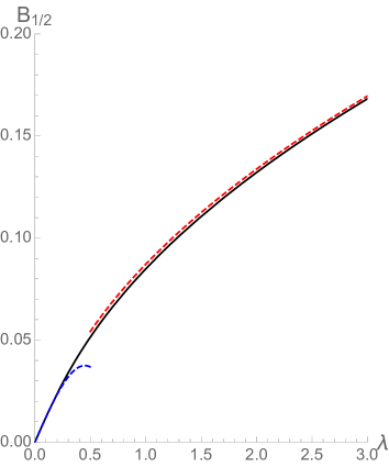
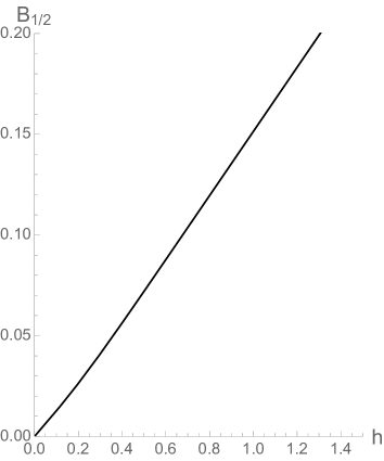
Figure 2: Left panel: plot of (6.1) (black curve) and its weak/strong coupling expansions (142) and (145) (blue/red curves) as functions of the ’t Hooft coupling. Right panel: plot of (6.1) as function of the interpolating function of ABJM integrability.

As a check, we perform a weak coupling expansion. In the region $\lambda\ll 1$ the inversion of (125) delivers Marino:2009jd

$$\kappa=8\pi\lambda+\frac{8\pi^{3}}{3}\lambda^{3}-\frac{14\pi^{5}}{15}\lambda^{5}+\frac{346\pi^{7}}{315}\lambda^{7}+O(\lambda^{9})$$ (141)

and one obtains

$$B_{1/2}=\frac{\lambda}{8}-\frac{\pi^{2}\lambda^{3}}{48}+O(\lambda^{5})\,.$$ (142)

It reproduces the known coefficients in calculations up to three loops Griguolo:2012iq ; Bianchi:2014laa ; Bianchi:2017svd . In the opposite regime $\lambda\gg 1$ one has Marino:2009jd

$$\kappa=e^{\pi\sqrt{2\lambda}}\big{(}1+O(\lambda^{-1/2},e^{-2\pi\sqrt{2\lambda}})\big{)}$$ (143)

and from

$$\Pi\left(\frac{1-a^{2}}{1+ab}\left|\frac{\left(a^{2}-1\right)\left(b^{2}-1\right)}{(1+ab)^{2}}\right.\right)=-\frac{3i}{8}\kappa\log\kappa+\frac{\pi}{16}\kappa+O(\log\kappa)\,,\qquad\kappa\to\infty$$ (144)

it follows that

$$B_{1/2}=\frac{\sqrt{\lambda}}{2\sqrt{2}\pi}-\frac{1}{4\pi^{2}}+O(\lambda^{-1/2})\,,\qquad\lambda\gg 1\,.$$ (145)

This agrees with the classical and one-loop order in calculations in string theory Forini:2012bb ; Correa:2014aga ; Aguilera-Damia:2014bqa .

6.2 Interpolating function

A conjecture for the exact expression of the interpolating function of ABJM integrability was put forward in Gromov:2014eha . The proposal takes the form of an implicit equation

$$\lambda=\frac{\sinh(2\pi h(\lambda))}{2\pi}{}_{3}F_{2}\left(\frac{1}{2},\frac{1}{2},\frac{1}{2};1,\frac{3}{2};-\sinh^{2}(2\pi h(\lambda))\right)$$ (146)

based on the similarity between two exact results in ABJM: the slope function Basso:2011rs describing the small-spin limit of $SL(2)$ operators as derived via integrability Cavaglia:2014exa and the $\frac{1}{6}$BPS Wilson loop (124) via localization. In particular, one recognizes that $h(\lambda)$ should have a very simple expression in terms of the localization effective coupling (125)

$$\kappa(\lambda)=4\sinh(2\pi h(\lambda))$$ (147)

where the ’t Hooft coupling is absorbed in these two “couplings” and does not appear explicitly. As suggested in Gromov:2014eha , a rigorous derivation of (146) would require the comparison of the Bremsstrahlung function obtained as function of $h(\lambda)$ from thermodynamic Bethe ansatz equations Bombardelli:2009xz ; Gromov:2009at or quantum spectral curve method Bombardelli:2017vhk and the localization prediction (6.1) function of $\kappa(\lambda)$, paralleling a similar derivation done in $\mathcal{N}=4$ SYM Correa:2012hh . The comparison has not been done yet in ABJM because the integrability calculation is still lacking at the moment. Here we want instead to assume that (146) is correct and use the comparison to make an explicit prediction on the result of the integrability calculation of $B_{1/2}$. One should take (6.1) with $a,b$ given by (126)-(127) in terms of $\kappa$ and then trade $\kappa$ with the interpolating function using (147). This yields $B_{1/2}$ as an explicit function of $h(\lambda)$ (Figure 2, right panel) that will be very interesting to derive from first principles in the future.

Acknowledgements

We thank Marco Bianchi, João Caetano, Martina Cornagliotto, Luca Griguolo, Vladimir Kazakov, Madalena Lemos, Fedor Levkovich-Maslyuk, Andrea Mauri, Marco Meineri, Silvia Penati, Domenico Seminara and Diego Trancanelli for discussions and the authors of Bianchi:2018bke for sharing with us their results prior publication. We are particularly grateful to Luca Griguolo and Domenico Seminara for valuable help in the initial stage of the project. The work of LB is supported by Deutsche Forschungsgemeinschaft in Sonderforschungsbereich 676 “Particles, Strings, and the Early Universe” and by the European Union’s Horizon 2020 research and innovation programme under the Marie Sklodowska-Curie grant agreement No 749909. The work of MP is supported by “Della Riccia Foundation” grant and by the European Research Council (Programme “Ideas” ERC-2012-AdG 320769 AdS-CFT-solvable). EV acknowledges financial support by FAPESP grants 2014/18634-9 and 2016/09266-1 and he thanks Yunfeng Jiang and ETH Zurich for hospitality while this project was in preparation.

Appendix A Conventions

The $\frac{1}{6}$BPS Wilson line breaks the $SU(4)$ R-symmetry down to $SU(2)\times SU(2)\times U(1)$. In particular the $SU(4)$ fundamental indices are split as follows

$$I=(a,\dot{a})$$ (148)

where $a$ is a fundamental index of the first $SU(2)$ factor and $\dot{a}$ of the second one. Those are raised and lowered by the action of epsilon tensors with the following conventions:

$$\epsilon^{12}=\epsilon^{\dot{1}\dot{2}} =1 \epsilon_{12} =\epsilon_{\dot{1}\dot{2}}=-1$$ (149)

such that

$$\epsilon^{ab}\epsilon_{bc} =\delta^{a}_{c} \epsilon^{\dot{a}\dot{b}}\epsilon_{\dot{b}\dot{c}} =\delta^{\dot{a}}_{\dot{c}}\,.$$ (150)

The spinor contractions and the conventions of the raising and lowering spinorial indices are as follows

$$\chi\bar{\chi}\equiv\chi^{\alpha}\bar{\chi}_{\alpha}\qquad\chi^{\alpha}=\epsilon^{\alpha\beta}\chi_{\beta}\qquad\epsilon^{\alpha\beta}\epsilon_{\beta\gamma}=\delta^{\alpha}_{\gamma}\qquad\epsilon^{12}=-\epsilon_{12}=1\,.$$ (151)

We work in the Euclidean space parametrized by the vector $x^{\mu}=\{x^{1},x^{2},x^{3}\}$ with $\gamma$ matrices

$${(\gamma^{\mu})_{\alpha}}^{\beta}=(\sigma^{1},\sigma^{2},-\sigma^{3})$$ (152)

satisfying the Clifford algebra $\{\gamma^{\mu},\gamma^{\nu}\}=2\delta^{\mu\nu}\mathbb{1}$ and obeying the following relation

$${(\gamma^{\mu})^{\alpha}}_{\beta}=\epsilon^{\alpha\gamma}\epsilon_{\beta\delta}{(\gamma^{\mu})_{\gamma}}^{\delta}\quad\Longrightarrow\quad{(\gamma^{\mu})^{\alpha}}_{\beta}=(\sigma^{1},-\sigma^{2},-\sigma^{3})$$ (153)

where $\sigma$’s are the Pauli matrices. When gamma matrices are involved and no spinor indices are specified the following convention is assumed

$$\chi\gamma^{\mu}\bar{\chi}=\chi^{\alpha}{(\gamma^{\mu})_{\alpha}}^{\beta}\bar{\chi}_{\beta}\,.$$ (154)

In this paper for the straight line we use the $\pm$ basis, then it is useful to write down the gamma matrices projected in this basis

$${(\gamma^{\mu}_{\pm\text{ basis}})_{\pm}}^{\pm}=\{\sigma_{3},\sigma_{2},-\sigma_{1}\}\,.$$ (155)

Appendix B Bremsstrahlung functions and operator insertions

In this section we justify and motivate the introduction of an absolute value in the prescription for computing $B_{1/6}^{\theta}$ in terms of the latitude Wilson loops. All expectation values in this appendix are at framing 0, hence the subscript is suppressed. Consider first the generalized cusp described in section 2.3. When taking a double derivative with respect to the internal angle $\theta$, in our notation we get a the following combination of defect two-point functions

$$\left.\frac{\partial^{2}}{\partial\theta^{2}}\log\braket{\mathcal{W}_{B}[C]}\right|_{\theta=0}=\frac{1}{4}\int_{0}^{\infty}d\tau_{1}\int_{\tau_{1}}^{\infty}d\tau_{2}\left(\braket{\mathbb{O}^{2\dot{1}}(\tau_{1})\bar{\mathbb{O}}^{\dot{2}1}(\tau_{2})}_{\mathcal{W}}+\braket{\bar{\mathbb{O}}^{\dot{2}1}(\tau_{1})\mathbb{O}^{2\dot{1}}(\tau_{2})}_{\mathcal{W}}\right)$$ (156)

where one should keep in mind that $\mathbb{O}^{2\dot{1}}=\frac{4\pi i}{k}C_{1}\bar{C}^{3}$. Although the symmetry fixes

$$\braket{\mathbb{O}^{2\dot{1}}(\tau_{1})\bar{\mathbb{O}}^{\dot{2}1}(\tau_{2})}_{\mathcal{W}}=\braket{\bar{\mathbb{O}}^{\dot{2}1}(\tau_{1})\mathbb{O}^{2\dot{1}}(\tau_{2})}_{\mathcal{W}}$$ (157)

let us suppose for a second that they are determined by the general form (62) with two different coefficients $c_{s}$ and $\bar{c}_{s}$. Therefore we get

$$\left.\frac{\partial^{2}}{\partial\theta^{2}}\log\braket{\mathcal{W}_{B}[C]}\right|_{\theta=0}=-\frac{c_{s}+\bar{c}_{s}}{4}\int_{0}^{\infty}d\tau_{1}\int_{\tau_{1}}^{\infty}d\tau_{2}\frac{1}{|\tau_{12}|^{2}}\,.$$ (158)

Switching to the cylinder parametrization (see Aguilera-Damia:2014bqa ; Bianchi:2017ozk ) we get

$$\left.\frac{\partial^{2}}{\partial\theta^{2}}\log\braket{\mathcal{W}_{B}[C]}\right|_{\theta=0}=-\frac{c_{s}+\bar{c}_{s}}{4}\int_{-\infty}^{\infty}d\tau_{1}\int_{\tau_{1}}^{\infty}d\tau_{2}\frac{1}{2(\cosh\tau_{12}-1)}=T\ \frac{c_{s}+\bar{c}_{s}}{4}$$ (159)

where $T$ is an overall divergence corresponding to the integral $\int_{-\infty}^{\infty}d\tau$. From that, using the same arguments of Aguilera-Damia:2014bqa ; Bianchi:2017ozk we can write

$$B^{\theta}_{1/6}=-\frac{1}{2T}\left.\frac{\partial^{2}}{\partial\theta^{2}}\log\braket{\mathcal{W}_{B}[C]}\right|_{\theta=0}=-\frac{c_{s}+\bar{c}_{s}}{8}\,.$$ (160)

On the other hand, when we consider the derivative of the latitude Wilson loop of section 2.1 we have

$$\left.\frac{\partial^{2}\log\braket{\mathcal{W}_{B}(\nu)}}{\partial\theta_{0}^{2}}\right|_{\theta_{0}=0}\\ =-\frac{1}{4}\int_{0}^{2\pi}d\tau_{1}\int_{\tau_{1}}^{2\pi}d\tau_{2}\left(e^{i\tau_{12}}\braket{\mathbb{O}^{2\dot{1}}(\tau_{1})\bar{\mathbb{O}}^{\dot{2}1}(\tau_{2})}_{\mathcal{W}}+e^{-i\tau_{12}}\braket{\bar{\mathbb{O}}^{\dot{2}1}(\tau_{1})\mathbb{O}^{2\dot{1}}(\tau_{2})}_{\mathcal{W}}\right)$$ (161)

which gives

$$\left.\frac{\partial^{2}\log\braket{\mathcal{W}_{B}(\nu)}}{\partial\theta_{0}^{2}}\right|_{\theta_{0}=0}=-\frac{\pi}{2}\int_{0}^{2\pi}d\tau_{1}\int_{\tau_{1}}^{2\pi}d\tau_{2}\left(\frac{e^{i\tau_{12}}c_{s}+e^{-i\tau_{12}}\bar{c}_{s}}{2(1-\cos\tau_{12})}\right)\,.$$ (162)

This gives a real and an imaginary contribution

$$\left.\frac{\partial^{2}\log\braket{\mathcal{W}_{B}(\nu)}}{\partial\theta_{0}^{2}}\right|_{\theta_{0}=0}=-\frac{\pi}{2}\int_{0}^{2\pi}d\tau_{1}\int_{\tau_{1}}^{2\pi}d\tau_{2}\left(\frac{(c_{s}+\bar{c}_{s})\cos\tau_{12}+i(c_{s}-\bar{c}_{s})\sin\tau_{12}}{2(1-\cos\tau_{12})}\right)\,.$$ (163)

As we mentioned $c_{s}=\bar{c}_{s}$, but since $(c_{s}-\bar{c}_{s})$ multiplies a divergent integral the overlapping of these effects may produce an anomaly-like contribution in equation (163). The perturbative computation of Bianchi:2018bke actually shows that this is indeed the case. To avoid this issue and recover the expression for the Bremsstrahlung function in equation (160) we combine (163) with its complex conjugate, so that the imaginary part disappears

$$\frac{1}{2}\left(\left.\frac{\partial^{2}\log\braket{\mathcal{W}_{B}(\nu)}}{\partial\theta_{0}^{2}}\right|_{\theta_{0}=0}+\left.\frac{\partial^{2}\log\braket{\hat{\mathcal{W}}_{B}(\nu)}}{\partial\theta_{0}^{2}}\right|_{\theta_{0}=0}\right)=-\frac{\pi^{2}}{2}(c_{s}+\bar{c}_{s})=-\pi^{2}c_{s}\,.$$ (164)

Therefore, reinstating the subscript for framing 0 we conclude

$$B^{\theta}_{1/6}=\frac{1}{4\pi^{2}}\Big{.}\partial_{\nu}\log|\langle\mathcal{W}_{B}(\nu)\rangle_{0}|\Big{|}_{\nu=1}\,.$$ (165)

Appendix C The $su(1,1|1)$ subalgebra

We start from the $osp(6|4)$ supersymmetry algebra, which contains the three-dimensional conformal algebra

$$[P^{\mu},K^{\nu}] =-2\delta^{\mu\nu}D-2M^{\mu\nu} [D,P^{\mu}] =P^{\mu} [D,K^{\mu}] =-K^{\mu}$$ (166)

$$[M^{\mu\nu},M^{\rho\sigma}] =\delta^{\sigma[\mu}M^{\nu]\rho}+\delta^{\rho[\nu}M^{\mu]\sigma} [P^{\mu},M^{\nu\rho}] =\delta^{\mu[\nu}P^{\rho]} [K^{\mu},M^{\nu\rho}] =\delta^{\mu[\nu}K^{\rho]}\,,$$ (167)

the $SU(4)$ generators

$$[{J_{I}}^{J},{J_{K}}^{L}]=\delta_{I}^{L}{J_{K}}^{J}-\delta^{J}_{K}{J_{I}}^{L}$$ (168)

and the fermionic generators $Q^{IJ}_{\alpha}$ and $S^{IJ}_{\alpha}$

$$\{Q^{IJ}_{\alpha},Q^{KL\beta}\} =2\epsilon^{IJKL}{(\gamma^{\mu})_{\alpha}}^{\beta}P_{\mu}\qquad\{S^{IJ}_{\alpha},S^{KL\beta}\}=2\epsilon^{IJKL}{(\gamma^{\mu})_{\alpha}}^{\beta}K_{\mu}$$ (169)

$$\{Q^{IJ}_{\alpha},S^{KL\beta}\} =i\epsilon^{IJKL}({(\gamma^{\mu\nu})_{\alpha}}^{\beta}M_{\mu\nu}+2\delta_{\alpha}^{\beta}D)+2i\delta_{\alpha}^{\beta}\epsilon^{KLMN}(\delta_{M}^{J}{J_{N}}^{I}-\delta_{M}^{I}{J_{N}}^{J})$$ (170)

with the reality condition $\bar{Q}_{IJ\alpha}=\frac{1}{2}\epsilon_{IJKL}Q^{KL}_{\alpha}$. Mixed commutators are

$$[D,Q^{IJ}_{\alpha}] =\frac{1}{2}Q^{IJ}_{\alpha} [D,S^{IJ}_{\alpha}] =-\frac{1}{2}S^{IJ}_{\alpha}$$ (171)

$$[M^{\mu\nu},Q^{IJ}_{\alpha}] =-\frac{1}{2}{(\gamma^{\mu\nu})_{\alpha}}^{\beta}Q^{IJ}_{\beta} [M^{\mu\nu},S^{IJ}_{\alpha}] =-\frac{1}{2}{(\gamma^{\mu\nu})_{\alpha}}^{\beta}S^{IJ}_{\beta}$$ (172)

$$[K^{\mu},Q_{\alpha}^{IJ}] =i{(\gamma^{\mu})_{\alpha}}^{\beta}S^{IJ}_{\beta} [P^{\mu},S^{IJ}_{\alpha}] =i{(\gamma^{\mu})_{\alpha}}^{\beta}Q^{IJ}_{\beta}$$ (173)

$$[{J_{I}}^{J},Q^{KL}_{\alpha}] =\delta_{I}^{K}Q^{JL}_{\alpha}+\delta_{I}^{L}Q^{KJ}_{\alpha}-\frac{1}{2}\delta_{I}^{J}Q^{KL}_{\alpha} [{J_{I}}^{J},S^{KL}_{\alpha}] =\delta_{I}^{K}S^{JL}_{\alpha}+\delta_{I}^{L}S^{KJ}_{\alpha}-\frac{1}{2}\delta_{I}^{J}S^{KL}_{\alpha}\,.$$ (174)

The $su(1,1|1)$ subalgebra generated by $\{D,P,K,J;Q,\bar{Q},S,\bar{S}\}$ is preserved by the $\frac{1}{6}$BPS Wilson line, with the identifications

$$P \equiv P_{1} K \equiv K_{1} J \equiv{J_{1}}^{1}+{J_{2}}^{2}-iM^{23}$$ (175)

$$Q \equiv Q^{12}_{+} \bar{Q} \equiv Q^{34}_{-} S \equiv-iS^{12}_{+} \bar{S} \equiv iS^{34}_{-}\,.$$ (176)

The $su(1,1)$ commutation relations are

$$[P,K] =-2D [D,P] =P [D,K] =-K\,.$$ (177)

The anticommutation relations for the fermionic generators read

$$\{Q,\bar{Q}\} =2P \{S,\bar{S}\} =2K$$ (178)

$$\{Q,\bar{S}\} =2D-2J \{S,\bar{Q}\} =2D+2J$$ (179)

and mixed commutators

$$[D,Q] =\frac{1}{2}Q [D,\bar{Q}] =\frac{1}{2}\bar{Q} [D,S] =-\frac{1}{2}S [D,\bar{S}] =-\frac{1}{2}\bar{S}$$ (180)

$$[K,Q] =S [K,\bar{Q}] =\bar{S} [P,S] =-Q [P,\bar{S}] =-\bar{Q}$$ (181)

$$[J,Q] =\frac{1}{2}Q [J,\bar{Q}] =-\frac{1}{2}\bar{Q} [J,S] =\frac{1}{2}S [J,\bar{S}] =-\frac{1}{2}\bar{S}\,.$$ (182)

C.1 Representations of $su(1,1|1)$

We briefly review the classification of long and short multiplets of $su(1,1|1)$. The algebra is characterized by two Dynkin labels $[\Delta,j]$ associated to the Cartan generators of the subalgebra $su(1,1)\oplus u(1)$. The supercharges carry the following charges

$$Q \quad[\tfrac{1}{2},\tfrac{1}{2}] \bar{Q} \quad[\tfrac{1}{2},-\tfrac{1}{2}] S \quad[-\tfrac{1}{2},\tfrac{1}{2}] \bar{S} \quad[-\tfrac{1}{2},\tfrac{1}{2}]\,.$$ (183)

A highest weight state $\ket{\Delta,j}$ is defined by the condition

$$S\ket{\Delta,j}=\bar{S}\ket{\Delta,j}=0$$ (184)

and a long multiplet $\mathcal{A}_{\Delta,j}$ can be easily built by acting on it with the supercharges $Q$ and $\bar{Q}$

There are then two possible shortening conditions, generating two $\frac{1}{2}$BPS multiplets

$$j >0 Q\ket{\Delta,j}=0\quad \Rightarrow\quad\Delta=j \mathcal{B}_{j}$$ (185)

$$j <0 \bar{Q}\ket{\Delta,j}=0\quad \Rightarrow\quad\Delta=-j \bar{\mathcal{B}}_{j}$$ (186)

Those multiplets contain only two operators (besides the infinite tower of conformal descendants)

and the long multiplet at the unitarity bound simply decomposes as

$$j >0 \mathcal{A}_{j,j} =\mathcal{B}_{j}\oplus\mathcal{B}_{j+\frac{1}{2}}$$ (187)

$$j <0 \mathcal{A}_{-j,j} =\bar{\mathcal{B}}_{j}\oplus\bar{\mathcal{B}}_{j-\frac{1}{2}}\,.$$ (188)

Appendix D SUSY transformations

In our conventions the $\mathcal{N}=6$ supersymmetry transformations for the fundamental fields read

$$\delta C_{I} =-\theta_{IJ}\bar{\psi}^{J}$$

$$\delta\bar{C}^{I} =-\bar{\theta}^{IJ}\psi_{J}$$

$$\delta\psi_{I}^{\alpha} =-2\theta_{IJ}^{\beta}{(\gamma^{\mu})_{\beta}}^{\alpha}D_{\mu}\bar{C}^{J}+\frac{4\pi}{k}\theta_{IJ}^{\alpha}(\bar{C}^{J}C_{K}\bar{C}^{K}-\bar{C}^{K}C_{K}\bar{C}^{J})+\frac{8\pi}{k}\theta_{KL}^{\alpha}\bar{C}^{K}C_{I}\bar{C}^{L}$$

$$\delta\bar{\psi}^{I}_{\alpha} =-2\bar{\theta}^{IJ\,\beta}(\gamma^{\mu})_{\beta\alpha}D_{\mu}C_{J}+\frac{4\pi}{k}\bar{\theta}^{IJ}_{\alpha}(C_{K}\bar{C}^{K}C_{J}-C_{J}\bar{C}^{K}C_{K})+\frac{8\pi}{k}\bar{\theta}^{KL}_{\alpha}C_{L}\bar{C}^{I}C_{K}$$

$$\delta A_{\mu} =-\frac{2\pi i}{k}(\bar{\theta}^{IJ}\gamma_{\mu}C_{I}\psi_{J}+\theta_{IJ}\gamma_{\mu}\bar{\psi}^{I}\bar{C}^{J})$$

$$\delta\hat{A}_{\mu} =-\frac{2\pi i}{k}(\bar{\theta}^{IJ}\gamma_{\mu}\psi_{J}C_{I}+\theta_{IJ}\gamma_{\mu}\bar{C}^{J}\bar{\psi}^{I})\,.$$ (189)

The action of the supercharge $Q^{IJ}_{\alpha}$ can be obtained by applying of the differential operator

$$Q^{IJ}_{\alpha}=\frac{\partial}{\partial\theta_{IJ}^{\alpha}}$$ (190)

and using the reality condition $\bar{\theta}^{IJ}=\frac{1}{2}\epsilon^{IJKL}\theta_{KL}$ with $\epsilon^{1234}=1$.

D.1 Preserved SUSY transformations

From the transformations (189) we extract the variation of the fundamental fields under the preserved supercharges $Q$ and $\bar{Q}$

$$QC_{a} =\epsilon_{ab}\bar{\psi}_{+}^{b} QC_{\dot{a}} =0 Q\bar{C}^{a} =0 Q\bar{C}^{\dot{a}} =\epsilon^{\dot{a}\dot{b}}\psi_{\dot{b}}^{-}$$ (191)

$$\bar{Q}C_{a} =0 \bar{Q}C_{\dot{a}} =\epsilon_{\dot{a}\dot{b}}\bar{\psi}^{\dot{b}}_{-} \bar{Q}\bar{C}^{a} =-\epsilon^{ab}\psi_{b}^{+} \bar{Q}\bar{C}^{\dot{a}} =0$$ (192)

$$Q\psi_{a}^{+} =2\epsilon_{ab}\mathcal{D}_{\tau}\bar{C}^{b} Q\psi_{a}^{-} =-2i\epsilon_{ab}D\bar{C}^{b} Q\psi_{\dot{a}}^{+} =\frac{8\pi}{k}\epsilon_{ab}\bar{C}^{a}C_{\dot{a}}\bar{C}^{b} Q\psi_{\dot{a}}^{-} =0$$ (193)

$$Q\bar{\psi}^{a}_{+} =0 Q\bar{\psi}^{a}_{-} =-\frac{8\pi}{k}\epsilon^{\dot{a}\dot{b}}{C}_{\dot{a}}\bar{C}^{a}{C}_{\dot{b}} Q\bar{\psi}^{\dot{a}}_{+} =-2i\epsilon^{\dot{a}\dot{b}}DC_{\dot{b}} Q\bar{\psi}^{\dot{a}}_{-} =-2\epsilon^{\dot{a}\dot{b}}\mathcal{D}_{\tau}C_{\dot{b}}$$ (194)

$$\bar{Q}\psi_{a}^{+} =0 \bar{Q}\psi_{a}^{-} =-\frac{8\pi}{k}\epsilon_{\dot{a}\dot{b}}\bar{C}^{\dot{a}}C_{a}\bar{C}^{\dot{b}} \bar{Q}\psi_{\dot{a}}^{+} =2i\epsilon_{\dot{a}\dot{b}}\bar{D}\bar{C}^{\dot{b}} \bar{Q}\psi_{\dot{a}}^{-} =-2\epsilon_{\dot{a}\dot{b}}\mathcal{D}_{\tau}\bar{C}^{\dot{b}}\!\!\!$$ (195)

$$\bar{Q}\bar{\psi}^{a}_{+} =-2\epsilon^{ab}\mathcal{D}_{\tau}C_{b} \bar{Q}\bar{\psi}^{a}_{-} =-2i\epsilon^{ab}\bar{D}C_{b} \bar{Q}\bar{\psi}^{\dot{a}}_{+} =\frac{8\pi}{k}\epsilon^{ab}{C}_{a}\bar{C}^{\dot{a}}{C}_{b} \bar{Q}\bar{\psi}^{\dot{a}}_{-} =0$$ (196)

$$QA_{1} =\frac{2\pi i}{k}(\epsilon^{\dot{a}\dot{b}}C_{\dot{a}}\psi_{\dot{b}}^{-}+\epsilon_{ab}\bar{\psi}_{+}^{a}\bar{C}^{b}) \bar{Q}A_{1} =\frac{2\pi i}{k}(-\epsilon_{\dot{a}\dot{b}}\bar{\psi}^{\dot{a}}_{-}\bar{C}^{\dot{b}}+\epsilon^{ab}C_{a}\psi^{+}_{b})$$ (197)

where

$$\mathcal{D}_{\tau}C_{a} =\partial_{\tau}C_{a}+i\mathcal{L}_{B}C_{a}-iC_{a}\hat{\mathcal{L}}_{B} \mathcal{D}_{\tau}\bar{C}^{a} =\partial_{\tau}\bar{C}^{a}+i\hat{\mathcal{L}}_{B}\bar{C}^{a}-i\bar{C}^{a}{\mathcal{L}_{B}}$$ (198)

$$D =D_{2}-iD_{3} \bar{D} =D_{2}+iD_{3}\,.$$ (199)

From the supersymmetry transformations it is clear that the insertion of a single scalar field is BPS and one can check for consistency that

$$\bar{Q}QC_{a} =\{Q,\bar{Q}\}C_{a}=-2\mathcal{D}_{\tau}C_{a}\qquad\qquad\,Q\bar{Q}C_{\dot{a}}=\{Q,\bar{Q}\}C_{\dot{a}}=-2\mathcal{D}_{\tau}C_{\dot{a}}$$ (200)

$$\bar{Q}Q\bar{C}^{\dot{a}} =\{Q,\bar{Q}\}\bar{C}^{\dot{a}}=-2\mathcal{D}_{\tau}\bar{C}^{\dot{a}}\qquad\qquad Q\bar{Q}\bar{C}^{a}=\{Q,\bar{Q}\}\bar{C}^{a}=-2\mathcal{D}_{\tau}\bar{C}^{a}\,.$$ (201)

D.2 Broken SUSY transformations

In section 3.2 we need to compute the variation of the connection $\mathcal{L}_{B}$ under the broken generator $\mathfrak{Q}$. To do this we need to consider their action on the scalars and on the parallel component of the gauge field:

$$\mathfrak{Q}C_{a} =0 \mathfrak{Q}C_{\dot{a}} =\epsilon_{\dot{a}\dot{b}}\bar{\psi}^{\dot{b}}_{+} \mathfrak{Q}\bar{C}^{a} =\epsilon^{ab}\psi_{b}^{-} \mathfrak{Q}\bar{C}^{\dot{a}} =0$$ (202)

$$\mathfrak{Q}A_{1} =\frac{2\pi i}{k}\left(\epsilon^{ab}C_{a}\psi^{-}_{b}+\epsilon_{\dot{a}\dot{b}}\bar{\psi}_{+}^{\dot{a}}\bar{C}^{\dot{b}}\right)\,.$$ (203)

Furthermore in section 3.3 and 4.3 and we need the action of the supercharges $\mathfrak{Q}^{a\dot{a}}$ on the fundamental fields. For the scalars

$$\mathfrak{Q}^{a\dot{a}}C_{b} =-\delta^{a}_{b}\bar{\psi}_{+}^{\dot{a}} \mathfrak{Q}^{a\dot{a}}C_{\dot{b}} =\delta^{\dot{a}}_{\dot{b}}\bar{\psi}_{+}^{a} \mathfrak{Q}^{a\dot{a}}\bar{C}^{b} =-\epsilon^{ab}\epsilon^{\dot{a}\dot{b}}\psi^{-}_{\dot{b}} \mathfrak{Q}^{a\dot{a}}\bar{C}^{\dot{b}} =\epsilon^{ab}\epsilon^{\dot{a}\dot{b}}\psi_{b}^{-}$$ (204)

For the fermions

$$\mathfrak{Q}^{b\dot{b}}\psi^{+}_{a} =-\delta_{a}^{b}2\mathcal{D}_{\tau}\bar{C}^{\dot{b}}-\tfrac{8\pi}{k}[\delta_{a}^{b}(\bar{C}^{c}C_{c}\bar{C}^{\dot{b}}-\bar{C}^{\dot{b}}C_{c}\bar{C}^{c})+\bar{C}^{\dot{b}}C_{a}\bar{C}^{b}-\bar{C}^{b}C_{a}\bar{C}^{\dot{b}}]$$ (205)

$$\mathfrak{Q}^{b\dot{b}}\psi^{-}_{a} =2i\delta_{a}^{b}D\bar{C}^{\dot{b}}$$ (206)

$$\mathfrak{Q}^{b\dot{b}}\psi^{+}_{\dot{a}} =\delta_{\dot{a}}^{\dot{b}}2\mathcal{D}_{\tau}\bar{C}^{b}+\tfrac{8\pi}{k}[\delta_{\dot{a}}^{\dot{b}}(\bar{C}^{c}C_{c}\bar{C}^{b}-\bar{C}^{b}C_{c}\bar{C}^{c})-\bar{C}^{\dot{b}}C_{\dot{a}}\bar{C}^{b}+\bar{C}^{b}C_{\dot{a}}\bar{C}^{\dot{b}}]$$ (207)

$$\mathfrak{Q}^{b\dot{b}}\psi^{-}_{\dot{a}} =-2i\delta_{\dot{a}}^{\dot{b}}D\bar{C}^{b}$$ (208)

$$\mathfrak{Q}^{b\dot{b}}\bar{\psi}_{-}^{a} =\epsilon^{ab}\epsilon^{\dot{a}\dot{b}}2\mathcal{D}_{\tau}C_{\dot{a}}-\tfrac{8\pi}{k}[\epsilon^{ab}\epsilon^{\dot{a}\dot{b}}(C_{\dot{c}}\bar{C}^{\dot{c}}C_{\dot{a}}-C_{\dot{a}}\bar{C}^{\dot{c}}C_{\dot{c}})+\epsilon^{cb}\epsilon^{\dot{c}\dot{b}}(C_{\dot{c}}\bar{C}^{a}C_{c}-C_{c}\bar{C}^{a}C_{\dot{c}})]$$ (209)

$$\mathfrak{Q}^{b\dot{b}}\bar{\psi}_{+}^{a} =2i\epsilon^{ab}\epsilon^{\dot{a}\dot{b}}DC_{\dot{a}}$$ (210)

$$\mathfrak{Q}^{b\dot{b}}\bar{\psi}_{-}^{\dot{a}} =-\epsilon^{ab}\epsilon^{\dot{a}\dot{b}}2\mathcal{D}_{\tau}C_{a}+\tfrac{8\pi}{k}[\epsilon^{ab}\epsilon^{\dot{a}\dot{b}}(C_{\dot{c}}\bar{C}^{\dot{c}}C_{a}-C_{a}\bar{C}^{\dot{c}}C_{\dot{c}})-\epsilon^{cb}\epsilon^{\dot{c}\dot{b}}(C_{\dot{c}}\bar{C}^{\dot{a}}C_{c}-C_{c}\bar{C}^{\dot{a}}C_{\dot{c}})]$$ (211)

$$\mathfrak{Q}^{b\dot{b}}\bar{\psi}_{+}^{\dot{a}} =-2i\epsilon^{ab}\epsilon^{\dot{a}\dot{b}}DC_{a}$$ (212)

and for the parallel component of the gauge field

$$\mathfrak{Q}^{b\dot{b}}A_{1}=-\frac{2\pi i}{k}(\epsilon^{ab}\epsilon^{\dot{a}\dot{b}}C_{a}\psi^{-}_{\dot{a}}-\epsilon^{ab}\epsilon^{\dot{a}\dot{b}}C_{\dot{a}}\psi^{-}_{a}+\bar{\psi}^{b}_{+}\bar{C}^{\dot{b}}-\bar{\psi}_{+}^{\dot{b}}\bar{C}^{b})\,.$$ (213)

One particular supersymmetry transformation that we need in section 4.3 is

$$\mathfrak{Q}^{a\dot{a}}\bar{\mathbb{F}} =-2\mathcal{D}_{\tau}\bar{\mathbb{O}}^{\dot{a}a}-\frac{4\pi i}{k}\epsilon^{\dot{a}\dot{b}}\bar{\psi}_{\alpha}^{a}\psi_{\dot{b}}^{\alpha}$$ (214)

$$-\tfrac{32\pi^{2}i}{k^{2}}[\epsilon^{\dot{a}\dot{b}}(C_{\dot{c}}\bar{C}^{\dot{c}}C_{\dot{b}}\bar{C}^{a}-C_{\dot{b}}\bar{C}^{\dot{c}}C_{\dot{c}}\bar{C}^{a})+\epsilon^{ac}\epsilon^{\dot{a}\dot{c}}\epsilon_{bd}(C_{\dot{c}}\bar{C}^{b}C_{c}\bar{C}^{d}-C_{c}\bar{C}^{b}C_{\dot{c}}\bar{C}^{d})$$

$$\phantom{-\tfrac{32\pi^{2}i}{k^{2}}}-\epsilon^{\dot{a}\dot{c}}(C_{\dot{c}}\bar{C}^{c}C_{c}\bar{C}^{a}-C_{\dot{c}}\bar{C}^{a}C_{c}\bar{C}^{c})+\epsilon^{\dot{b}\dot{c}}(C_{\dot{c}}\bar{C}^{\dot{a}}C_{\dot{b}}\bar{C}^{a}-C_{\dot{c}}\bar{C}^{a}C_{\dot{b}}\bar{C}^{\dot{a}})]\,.$$

References

- (1) V. Pestun et al., “Localization techniques in quantum field theories”, arXiv:1608.02952.
- (2) J. A. Minahan and K. Zarembo, “The Bethe ansatz for N=4 superYang-Mills”, JHEP 0303, 013 (2003), hep-th/0212208.
- (3) D. Correa, J. Henn, J. Maldacena and A. Sever, “An exact formula for the radiation of a moving quark in N=4 super Yang Mills”, JHEP 1206, 048 (2012), arXiv:1202.4455.
- (4) D. Correa, J. Maldacena and A. Sever, “The quark anti-quark potential and the cusp anomalous dimension from a TBA equation”, JHEP 1208, 134 (2012), arXiv:1203.1913.
- (5) N. Drukker, “Integrable Wilson loops”, JHEP 1310, 135 (2013), arXiv:1203.1617.
- (6) M. Cooke, A. Dekel and N. Drukker, “The Wilson loop CFT: Insertion dimensions and structure constants from wavy lines”, J. Phys. A50, 335401 (2017), arXiv:1703.03812.
- (7) S. Giombi, R. Roiban and A. A. Tseytlin, “Half-BPS Wilson loop and AdS2/CFT1”, Nucl. Phys. B922, 499 (2017), arXiv:1706.00756.
- (8) B. Fiol, B. Garolera and A. Lewkowycz, “Exact results for static and radiative fields of a quark in N=4 super Yang-Mills”, JHEP 1205, 093 (2012), arXiv:1202.5292.
- (9) V. Pestun, “Localization of the four-dimensional N=4 SYM to a two-sphere and 1/8 BPS Wilson loops”, JHEP 1212, 067 (2012), arXiv:0906.0638.
- (10) J. K. Erickson, G. W. Semenoff and K. Zarembo, “Wilson loops in N=4 supersymmetric Yang-Mills theory”, Nucl. Phys. B582, 155 (2000), hep-th/0003055.
- (11) N. Drukker and D. J. Gross, “An Exact prediction of N=4 SUSYM theory for string theory”, J. Math. Phys. 42, 2896 (2001), hep-th/0010274.
- (12) V. Pestun, “Localization of gauge theory on a four-sphere and supersymmetric Wilson loops”, Commun. Math. Phys. 313, 71 (2012), arXiv:0712.2824.
- (13) N. Gromov, F. Levkovich-Maslyuk and G. Sizov, “Analytic Solution of Bremsstrahlung TBA II: Turning on the Sphere Angle”, JHEP 1310, 036 (2013), arXiv:1305.1944.
- (14) N. Gromov and F. Levkovich-Maslyuk, “Quantum Spectral Curve for a cusped Wilson line in SYM”, JHEP 1604, 134 (2016), arXiv:1510.02098.
- (15) M. Bonini, L. Griguolo, M. Preti and D. Seminara, “Bremsstrahlung function, leading Lüscher correction at weak coupling and localization”, JHEP 1602, 172 (2016), arXiv:1511.05016.
- (16) O. Aharony, O. Bergman, D. L. Jafferis and J. Maldacena, “ superconformal Chern-Simons-matter theories, M2-branes and their gravity duals”, JHEP 0810, 091 (2008), arXiv:0806.1218.
- (17) N. Gromov and G. Sizov, “Exact Slope and Interpolating Functions in N=6 Supersymmetric Chern-Simons Theory”, Phys. Rev. Lett. 113, 121601 (2014), arXiv:1403.1894.
- (18) D. Gaiotto, S. Giombi and X. Yin, “Spin Chains in N=6 Superconformal Chern-Simons-Matter Theory”, JHEP 0904, 066 (2009), arXiv:0806.4589.
- (19) G. Grignani, T. Harmark and M. Orselli, “The SU(2) SU(2) sector in the string dual of N=6 superconformal Chern-Simons theory”, Nucl. Phys. B810, 115 (2009), arXiv:0806.4959.
- (20) T. Nishioka and T. Takayanagi, “On Type IIA Penrose Limit and N=6 Chern-Simons Theories”, JHEP 0808, 001 (2008), arXiv:0806.3391.
- (21) J. A. Minahan, O. Ohlsson Sax and C. Sieg, “Magnon dispersion to four loops in the ABJM and ABJ models”, J. Phys. A43, 275402 (2010), arXiv:0908.2463.
- (22) J. A. Minahan, O. Ohlsson Sax and C. Sieg, “Anomalous dimensions at four loops in N=6 superconformal Chern-Simons theories”, Nucl. Phys. B846, 542 (2011), arXiv:0912.3460.
- (23) M. Leoni, A. Mauri, J. A. Minahan, O. Ohlsson Sax, A. Santambrogio, C. Sieg and G. Tartaglino-Mazzucchelli, “Superspace calculation of the four-loop spectrum in N=6 supersymmetric Chern-Simons theories”, JHEP 1012, 074 (2010), arXiv:1010.1756.
- (24) T. McLoughlin, R. Roiban and A. A. Tseytlin, “Quantum spinning strings in : Testing the Bethe Ansatz proposal”, JHEP 0811, 069 (2008), arXiv:0809.4038.
- (25) M. C. Abbott, I. Aniceto and D. Bombardelli, “Quantum Strings and the Interpolating Function”, JHEP 1012, 040 (2010), arXiv:1006.2174.
- (26) C. Lopez-Arcos and H. Nastase, “Eliminating ambiguities for quantum corrections to strings moving in ”, Int. J. Mod. Phys. A28, 1350058 (2013), arXiv:1203.4777.
- (27) L. Bianchi, M. S. Bianchi, A. Bres, V. Forini and E. Vescovi, “Two-loop cusp anomaly in ABJM at strong coupling”, JHEP 1410, 013 (2014), arXiv:1407.4788.
- (28) A. Cavaglià, N. Gromov and F. Levkovich-Maslyuk, “On the Exact Interpolating Function in ABJ Theory”, JHEP 1612, 086 (2016), arXiv:1605.04888.
- (29) J. M. Maldacena, “Wilson loops in large N field theories”, Phys. Rev. Lett. 80, 4859 (1998), hep-th/9803002.
- (30) D. Berenstein and D. Trancanelli, “Three-dimensional N=6 SCFT’s and their membrane dynamics”, Phys. Rev. D78, 106009 (2008), arXiv:0808.2503.
- (31) N. Drukker, J. Plefka and D. Young, “Wilson loops in 3-dimensional N=6 supersymmetric Chern-Simons Theory and their string theory duals”, JHEP 0811, 019 (2008), arXiv:0809.2787.
- (32) B. Chen and J.-B. Wu, “Supersymmetric Wilson Loops in N=6 Super Chern-Simons-matter theory”, Nucl. Phys. B825, 38 (2010), arXiv:0809.2863.
- (33) N. Drukker and D. Trancanelli, “A Supermatrix model for N=6 super Chern-Simons-matter theory”, JHEP 1002, 058 (2010), arXiv:0912.3006.
- (34) V. Cardinali, L. Griguolo, G. Martelloni and D. Seminara, “New supersymmetric Wilson loops in ABJ(M) theories”, Phys. Lett. B718, 615 (2012), arXiv:1209.4032.
- (35) A. M. Polyakov, “Gauge Fields as Rings of Glue”, Nucl. Phys. B164, 171 (1980).
- (36) G. P. Korchemsky and A. V. Radyushkin, “Renormalization of the Wilson Loops Beyond the Leading Order”, Nucl. Phys. B283, 342 (1987).
- (37) N. Drukker, D. J. Gross and H. Ooguri, “Wilson loops and minimal surfaces”, Phys. Rev. D60, 125006 (1999), hep-th/9904191.
- (38) N. Drukker and V. Forini, “Generalized quark-antiquark potential at weak and strong coupling”, JHEP 1106, 131 (2011), arXiv:1105.5144.
- (39) L. Griguolo, D. Marmiroli, G. Martelloni and D. Seminara, “The generalized cusp in ABJ(M) N = 6 Super Chern-Simons theories”, JHEP 1305, 113 (2013), arXiv:1208.5766.
- (40) D. H. Correa, J. Aguilera-Damia and G. A. Silva, “Strings in Wilson loops in 6 super Chern-Simons-matter and bremsstrahlung functions”, JHEP 1406, 139 (2014), arXiv:1405.1396.
- (41) M. S. Bianchi, L. Griguolo, M. Leoni, S. Penati and D. Seminara, “BPS Wilson loops and Bremsstrahlung function in ABJ(M): a two loop analysis”, JHEP 1406, 123 (2014), arXiv:1402.4128.
- (42) M. S. Bianchi, L. Griguolo, A. Mauri, S. Penati, M. Preti and D. Seminara, “Towards the exact Bremsstrahlung function of ABJM theory”, JHEP 1708, 022 (2017), arXiv:1705.10780.
- (43) L. Bianchi, L. Griguolo, M. Preti and D. Seminara, “Wilson lines as superconformal defects in ABJM theory: a formula for the emitted radiation”, JHEP 1710, 050 (2017), arXiv:1706.06590.
- (44) M. S. Bianchi, L. Griguolo, M. Leoni, A. Mauri, S. Penati and D. Seminara, “Framing and localization in Chern-Simons theories with matter”, JHEP 1606, 133 (2016), arXiv:1604.00383.
- (45) A. Lewkowycz and J. Maldacena, “Exact results for the entanglement entropy and the energy radiated by a quark”, JHEP 1405, 025 (2014), arXiv:1312.5682.
- (46) A. Kapustin, B. Willett and I. Yaakov, “Exact Results for Wilson Loops in Superconformal Chern-Simons Theories with Matter”, JHEP 1003, 089 (2010), arXiv:0909.4559.
- (47) M. Marino and P. Putrov, “Exact Results in ABJM Theory from Topological Strings”, JHEP 1006, 011 (2010), arXiv:0912.3074.
- (48) N. Drukker, M. Marino and P. Putrov, “From weak to strong coupling in ABJM theory”, Commun. Math. Phys. 306, 511 (2011), arXiv:1007.3837.
- (49) A. Klemm, M. Marino, M. Schiereck and M. Soroush, “Aharony-Bergman-Jafferis-Maldacena Wilson loops in the Fermi gas approach”, Z. Naturforsch. A68, 178 (2013), arXiv:1207.0611.
- (50) M. S. Bianchi and A. Mauri, “ABJM -Bremsstrahlung at four loops and beyond”, JHEP 1711, 173 (2017), arXiv:1709.01089.
- (51) M. S. Bianchi and A. Mauri, “ABJM -Bremsstrahlung at four loops and beyond: non-planar corrections”, JHEP 1711, 166 (2017), arXiv:1709.10092.
- (52) M. Billò, V. Goncalves, E. Lauria and M. Meineri, “Defects in conformal field theory”, JHEP 1604, 091 (2016), arXiv:1601.02883.
- (53) C. Cordova, T. T. Dumitrescu and K. Intriligator, “Multiplets of Superconformal Symmetry in Diverse Dimensions”, arXiv:1612.00809.
- (54) P. Liendo and C. Meneghelli, “Bootstrap equations for = 4 SYM with defects”, JHEP 1701, 122 (2017), arXiv:1608.05126.
- (55) R. Blumenhagen, “N=2 supersymmetric W algebras”, Nucl. Phys. B405, 744 (1993), hep-th/9208069.
- (56) P. Di Vecchia, J. L. Petersen and H. B. Zheng, “N=2 Extended Superconformal Theories in Two-Dimensions”, Phys. Lett. 162B, 327 (1985).
- (57) G. Mussardo, G. Sotkov and M. Stanishkov, “N=2 SUPERCONFORMAL MINIMAL MODELS”, Int. J. Mod. Phys. A4, 1135 (1989).
- (58) M. Cornagliotto, M. Lemos and V. Schomerus, “Long Multiplet Bootstrap”, JHEP 1710, 119 (2017), arXiv:1702.05101.
- (59) A. L. Fitzpatrick, J. Kaplan, Z. U. Khandker, D. Li, D. Poland and D. Simmons-Duffin, “Covariant Approaches to Superconformal Blocks”, JHEP 1408, 129 (2014), arXiv:1402.1167.
- (60) M. A. Bandres, A. E. Lipstein and J. H. Schwarz, “Studies of the ABJM Theory in a Formulation with Manifest SU(4) R-Symmetry”, JHEP 0809, 027 (2008), arXiv:0807.0880.
- (61) S.-J. Rey, T. Suyama and S. Yamaguchi, “Wilson Loops in Superconformal Chern-Simons Theory and Fundamental Strings in Anti-de Sitter Supergravity Dual”, JHEP 0903, 127 (2009), arXiv:0809.3786.
- (62) K.-M. Lee and S. Lee, “1/2-BPS Wilson Loops and Vortices in ABJM Model”, JHEP 1009, 004 (2010), arXiv:1006.5589.
- (63) N. Beisert, B. Eden and M. Staudacher, “Transcendentality and Crossing”, J. Stat. Mech. 0701, P01021 (2007), hep-th/0610251.
- (64) N. Gromov and P. Vieira, “The all loop AdS4/CFT3 Bethe ansatz”, JHEP 0901, 016 (2009), arXiv:0807.0777.
- (65) M. Bonini, L. Griguolo, M. Preti and D. Seminara, “Surprises from the resummation of ladders in the ABJ(M) cusp anomalous dimension”, JHEP 1605, 180 (2016), arXiv:1603.00541.
- (66) M. Preti, “WiLE: a Mathematica package for weak coupling expansion of Wilson loops in ABJ(M) theory”, arXiv:1707.08108.
- (67) V. Forini, V. G. M. Puletti and O. Ohlsson Sax, “The generalized cusp in and more one-loop results from semiclassical strings”, J. Phys. A46, 115402 (2013), arXiv:1204.3302.
- (68) B. Fiol, E. Gerchkovitz and Z. Komargodski, “Exact Bremsstrahlung Function in Superconformal Field Theories”, Phys. Rev. Lett. 116, 081601 (2016), arXiv:1510.01332.
- (69) L. Bianchi, M. Meineri, R. C. Myers and M. Smolkin, “Rényi entropy and conformal defects”, JHEP 1607, 076 (2016), arXiv:1511.06713.
- (70) L. Bianchi, S. Chapman, X. Dong, D. A. Galante, M. Meineri and R. C. Myers, “Shape dependence of holographic Rényi entropy in general dimensions”, JHEP 1611, 180 (2016), arXiv:1607.07418.
- (71) M. Lemos, P. Liendo, M. Meineri and S. Sarkar, “Universality at large transverse spin in defect CFT”, arXiv:1712.08185.
- (72) S. Balakrishnan, T. Faulkner, Z. U. Khandker and H. Wang, “A General Proof of the Quantum Null Energy Condition”, arXiv:1706.09432.
- (73) X. Dong, “Shape Dependence of Holographic Rényi Entropy in Conformal Field Theories”, Phys. Rev. Lett. 116, 251602 (2016), arXiv:1602.08493.
- (74) S. Balakrishnan, S. Dutta and T. Faulkner, “Gravitational dual of the Rényi twist displacement operator”, Phys. Rev. D96, 046019 (2017), arXiv:1607.06155.
- (75) C. P. Herzog and K.-W. Huang, “Boundary Conformal Field Theory and a Boundary Central Charge”, JHEP 1710, 189 (2017), arXiv:1707.06224.
- (76) J. Aguilera-Damia, D. H. Correa and G. A. Silva, “Semiclassical partition function for strings dual to Wilson loops with small cusps in ABJM”, JHEP 1503, 002 (2015), arXiv:1412.4084.
- (77) M. S. Bianchi, “A note on multiply wound BPS Wilson loops in ABJM”, JHEP 1609, 047 (2016), arXiv:1605.01025.
- (78) M. S. Bianchi, L. Griguolo, A. Mauri, S. Penati and D. Seminara, “A matrix model for the latitude Wilson loop in ABJM theory”, arXiv:1802.07742.
- (79) M. Marino, “Chern-Simons theory, matrix integrals, and perturbative three manifold invariants”, Commun. Math. Phys. 253, 25 (2004), hep-th/0207096.
- (80) I. S. Gradshteyn and I. M. Ryzhik, “Table of integrals, series, and products”.
- (81) E. Vescovi, “Perturbative and non-perturbative approaches to string sigma-models in AdS/CFT”, https://edoc.hu-berlin.de/docviews/abstract.php?id=42898.
- (82) B. Basso, “An exact slope for AdS/CFT”, arXiv:1109.3154.
- (83) A. Cavaglià, D. Fioravanti, N. Gromov and R. Tateo, “Quantum Spectral Curve of the 6 Supersymmetric Chern-Simons Theory”, Phys. Rev. Lett. 113, 021601 (2014), arXiv:1403.1859.
- (84) D. Bombardelli, D. Fioravanti and R. Tateo, “TBA and Y-system for planar AdS(4)/CFT(3)”, Nucl. Phys. B834, 543 (2010), arXiv:0912.4715.
- (85) N. Gromov and F. Levkovich-Maslyuk, “Y-system, TBA and Quasi-Classical strings in AdS(4) x CP3”, JHEP 1006, 088 (2010), arXiv:0912.4911.
- (86) D. Bombardelli, A. Cavaglià, D. Fioravanti, N. Gromov and R. Tateo, “The full Quantum Spectral Curve for ”, JHEP 1709, 140 (2017), arXiv:1701.00473.