Increased Heat Transport in Ultra-Hot Jupiter Atmospheres Through
H₂ Dissociation/Recombination

Abstract

A new class of exoplanets is beginning to emerge: planets whose dayside atmospheres more closely resemble stellar atmospheres as most of their molecular constituents dissociate. The effects of the dissociation of these species will be varied and must be carefully accounted for. Here we take the first steps towards understanding the consequences of dissociation and recombination of molecular hydrogen (H₂) on atmospheric heat recirculation. Using a simple energy balance model with eastward winds, we demonstrate that H₂ dissociation/recombination can significantly increase the day–night heat transport on ultra-hot Jupiters (UHJs): gas giant exoplanets where significant H₂ dissociation occurs. The atomic hydrogen from the highly irradiated daysides of UHJs will transport some of the energy deposited on the dayside towards the nightside of the planet where the H atoms recombine into H₂; this mechanism bears similarities to latent heat. Given a fixed wind speed, this will act to increase the heat recirculation efficiency; alternatively, a measured heat recirculation efficiency will require slower wind speeds after accounting for H₂ dissociation/recombination.

1 Introduction

Most gas giant exoplanets have atmospheres dominated by molecular hydrogen (H₂). However, on planets where the temperature is sufficiently high, a significant fraction of the H₂ will thermally dissociate; one may call these planets ultra-hot Jupiters (UHJs). Only a handful of known planets have dayside temperatures this high, but the TESS mission is expected to discover hundreds more as it includes many early-type stars . These UHJs are an interesting intermediate between stars and cooler planets, and they will allow for useful tests of atmospheric models.

At these star-like temperatures, the H^- bound-free and free-free opacities should play an important role in the continuum atmospheric opacity which has recently been detected in dayside secondary eclipse spectra (Bell et al., 2017; Arcangeli et al., 2018). These recently reported detections of H^- opacity provide evidence that H₂ is dissociating in the atmospheres of gas giants at this temperature range. However, the thermodynamical effects of H₂ dissociation/recombination have yet to be explored.

Both theoretically (e.g. Perez-Becker & Showman, 2013; Komacek & Showman, 2016) and empirically (e.g. Zhang et al., 2018; Schwartz et al., 2017), we expect the day–night temperature contrast on hot Jupiters to increase with increasing stellar irradiation; temperature gradients $\mathrel{\mathchoice{\raise 0.0pt\hbox{\scalebox{0.8}{\raise 0.0pt\hbox{$\displaystyle\gtrsim$}}}}{\raise 0.0pt\hbox{\scalebox{0.8}{\raise 0.0pt\hbox{$\textstyle\gtrsim$}}}}{\raise 0.0pt\hbox{\scalebox{0.8}{\raise 0.0pt\hbox{$\scriptstyle\gtrsim$}}}}{\raise 0.0pt\hbox{\scalebox{0.8}{\raise 0.0pt\hbox{$\scriptscriptstyle\gtrsim$}}}}}1000$ K can be expected for UHJs. As temperatures vary drastically between day and night, the local thermal equilibrium (LTE) H₂ dissociation fraction will also vary. The recombination of H into H₂ is a remarkably exothermic process, releasing $q=$ 2.14$\times$10⁸ J kg^-1 (Dean, 1999); this is 100$\times$ more potent than the latent heat of condensation for water. For reference, latent heat is responsible for approximately half of the heat recirculation on Earth ($L/(c_{p}\Delta T)\sim 1$), while the effect of H₂ dissociation/recombination should be even stronger for UHJs ($q/(c_{p}\Delta T)\sim 10^{2}$).

Building on this intuition, we might expect that H will recombine into H₂ as gas carried by winds flows eastward from the sub-stellar point, significantly heating the eastern hemisphere of the planet. As the gas continues to flow around to the dayside, the H₂ will again dissociate and significantly cool the western hemisphere. A cartoon depicting this layout is shown in Figure 1. If unaccounted for while modelling a phasecurve, this may manifest itself as an “unphysically” large eastward offset as was previously reported for WASP-12b (Cowan et al., 2012).

“Top-Down” View

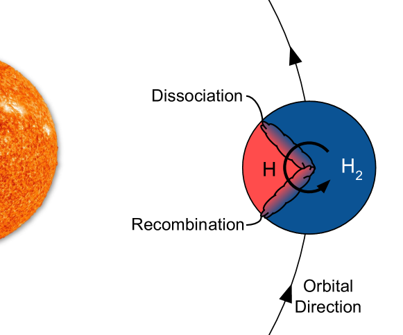
Figure 1: A cartoon showing a “top-down” view of the expected dissociation and recombination of H₂ on an ultra-hot Jupiter (UHJ). The orbital direction and the direction of winds on the planet are indicated with black arrows.

A large number of circulation models have been developed for studying exoplanet atmospheres, ranging from simple energy balance models (e.g. Cowan & Agol, 2011) to more advanced general circulation models (e.g. Showman et al., 2009; Rauscher & Menou, 2010; Amundsen et al., 2014; Zhang & Showman, 2017; Heng & Kitzmann, 2017; Dobbs-Dixon & Cowan, 2017). To our knowledge, however, no published general circulation models account for the cooling/heating due to the energies of H₂ dissociation/recombination (although some planet formation models do account for this, e.g. Berardo et al., 2017). Here we aim to qualitatively explore the effects of H₂ dissociation/recombination using a simple energy balance model adapted from that described by Cowan & Agol (2011), using code based on that implemented by Schwartz et al. (2017). We leave it to those with more advanced circulation models to explore this problem in a more rigorous and quantitative manner.

2 Energy Transport Model

2.1 Heating Terms

First, let $\epsilon$ be the energy per unit area of a parcel of gas. Ignoring H₂ dissociation/recombination and any internal heat sources, and assuming the gas parcel cools radiatively, energy conservation gives

$$\frac{d\epsilon}{dt}=F_{\rm in}-F_{\rm out},$$

with $F_{\rm{in}}$ and $F_{\rm{out}}$ given by

$$F_{\rm{in}}=(1-A_{B})F_{*}\sin{\theta}\max{\Big{(}\cos{\Phi(t)},0\Big{)}},$$

$$F_{\rm{out}}=\sigma T^{4}.$$

The planet’s Bond albedo is given by $A_{B}$, $\theta$ is the co-latitude of the gas parcel, $T$ is the temperature of the gas parcel, and $\sigma$ is the Stefan-Boltzmann constant. The incoming stellar flux is given by $F_{*}=\sigma T_{*,\rm{eff}}^{4}(R_{*}/a)^{2}$, where $T_{*,\rm{eff}}$ is the stellar effective temperature, $R_{*}$ is the stellar radius, and $a$ is the planet’s semi-major axis. The stellar hour angle, $\Phi(t)$, incorporates both advection and planetary rotation.

In order to include H₂ dissociation/recombination, we add a new term accounting for the energy flux from these effects. This can be done with

$$\frac{d\epsilon}{dt}=F_{\rm in}-F_{\rm out}-\frac{d\mathbb{Q}}{dt},$$ (1)

where the energy per unit area stored by H₂ dissociation is given by

$$\mathbb{Q}=q{\mathchoice{\raisebox{0.0pt}{$\displaystyle\chi$}}{\raisebox{0.0pt}{$\textstyle\chi$}}{\raisebox{0.0pt}{$\scriptstyle\chi$}}{\raisebox{0.0pt}{$\scriptscriptstyle\chi$}}}_{\rm H}\Sigma,$$

where $\Sigma$ is the mass per unit area of H and H₂ in the parcel of gas (in kg m^-2), $q=$ 2.14$\times$10⁸ J kg^-1 is the H₂ bond dissociation energy per unit mass at 0 K, and ${\mathchoice{\raisebox{0.0pt}{$\displaystyle\chi$}}{\raisebox{0.0pt}{$\textstyle\chi$}}{\raisebox{0.0pt}{$\scriptstyle\chi$}}{\raisebox{0.0pt}{$\scriptscriptstyle\chi$}}}_{\rm H}$ is the dissociation fraction of the gas. ${\mathchoice{\raisebox{0.0pt}{$\displaystyle\chi$}}{\raisebox{0.0pt}{$\textstyle\chi$}}{\raisebox{0.0pt}{$\scriptstyle\chi$}}{\raisebox{0.0pt}{$\scriptscriptstyle\chi$}}}_{\rm H}=1$ means the gas is completely dissociated (all atomic). Assuming the gas parcel is in hydrostatic equilibrium, we can use

$$\Sigma=\int_{z_{0}}^{\infty}\rho(z)dz=(P_{0}/g)$$

where $z_{0}$ is some reference height, $P_{0}$ is the atmospheric pressure corresponding to $z_{0}$, and $\rho$ is the density of the gas. This then allows us to rewrite $\mathbb{Q}$ as

$$\mathbb{Q}=(P_{0}/g)q{\mathchoice{\raisebox{0.0pt}{$\displaystyle\chi$}}{\raisebox{0.0pt}{$\textstyle\chi$}}{\raisebox{0.0pt}{$\scriptstyle\chi$}}{\raisebox{0.0pt}{$\scriptscriptstyle\chi$}}}_{\rm H}.$$

The time derivative of $\mathbb{Q}$ is then

$$\frac{d\mathbb{Q}}{dt}=(P_{0}/g)q\frac{d{\mathchoice{\raisebox{0.0pt}{$\displaystyle\chi$}}{\raisebox{0.0pt}{$\textstyle\chi$}}{\raisebox{0.0pt}{$\scriptstyle\chi$}}{\raisebox{0.0pt}{$\scriptscriptstyle\chi$}}}_{\rm H}}{dt}=(P_{0}/g)q\frac{d{\mathchoice{\raisebox{0.0pt}{$\displaystyle\chi$}}{\raisebox{0.0pt}{$\textstyle\chi$}}{\raisebox{0.0pt}{$\scriptstyle\chi$}}{\raisebox{0.0pt}{$\scriptscriptstyle\chi$}}}_{\rm H}}{dT}\biggr{\rvert}_{T}\frac{dT}{dt},$$ (2)

where we have assumed the gas parcel’s $P_{0}/g$ remains constant, and where we have made use of the chain rule to expand $d{\mathchoice{\raisebox{0.0pt}{$\displaystyle\chi$}}{\raisebox{0.0pt}{$\textstyle\chi$}}{\raisebox{0.0pt}{$\scriptstyle\chi$}}{\raisebox{0.0pt}{$\scriptscriptstyle\chi$}}}_{\rm H}/dt$.

We model the LTE H₂ dissociation fraction by solving the Saha equation as stated in Appendix A of Berardo et al. (2017) for ${\mathchoice{\raisebox{0.0pt}{$\displaystyle\chi$}}{\raisebox{0.0pt}{$\textstyle\chi$}}{\raisebox{0.0pt}{$\scriptstyle\chi$}}{\raisebox{0.0pt}{$\scriptscriptstyle\chi$}}}_{\rm H}$, assuming the atmosphere consists of only H and H₂:

$${\mathchoice{\raisebox{0.0pt}{$\displaystyle\chi$}}{\raisebox{0.0pt}{$\textstyle\chi$}}{\raisebox{0.0pt}{$\scriptstyle\chi$}}{\raisebox{0.0pt}{$\scriptscriptstyle\chi$}}}_{\rm H}(P,T)=\frac{n_{\rm H}}{n_{\rm H}+n_{\rm H_{2}}}=\frac{2}{1+\sqrt{1+4Y}},$$ (3)

where $n_{\rm H}$ and $n_{\rm H_{2}}$ are the number densities of H and H₂,

$$Y=\frac{T^{-3/2}\exp(q/2m_{\rm H}k_{\rm B}T)P}{2(\pi m_{\rm H})^{3/2}k_{\rm B}^{5/2}h^{-3}\Theta_{\rm rot}},$$

where $m_{\rm H}$ is the mass of the hydrogen atom, $k_{\rm B}$ is the Boltzmann constant, $h$ is the Planck constant, $\Theta_{\rm rot}=85.4$ K is rotational temperature of H₂ (Hill, 1986), $P$ is the gas pressure, and $T$ is the temperature of the gas (in K). The LTE dissociation fraction is plotted in the top panel of Figure 2.

We can then find $d{\mathchoice{\raisebox{0.0pt}{$\displaystyle\chi$}}{\raisebox{0.0pt}{$\textstyle\chi$}}{\raisebox{0.0pt}{$\scriptstyle\chi$}}{\raisebox{0.0pt}{$\scriptscriptstyle\chi$}}}_{\rm H}/dT$ using the chain rule:

$$\frac{d{\mathchoice{\raisebox{0.0pt}{$\displaystyle\chi$}}{\raisebox{0.0pt}{$\textstyle\chi$}}{\raisebox{0.0pt}{$\scriptstyle\chi$}}{\raisebox{0.0pt}{$\scriptscriptstyle\chi$}}}_{\rm H}}{dT}=\frac{d{\mathchoice{\raisebox{0.0pt}{$\displaystyle\chi$}}{\raisebox{0.0pt}{$\textstyle\chi$}}{\raisebox{0.0pt}{$\scriptstyle\chi$}}{\raisebox{0.0pt}{$\scriptscriptstyle\chi$}}}_{\rm H}}{dY}\frac{dY}{dT}.$$

After some simplification, we then determine

$$\frac{d{\mathchoice{\raisebox{0.0pt}{$\displaystyle\chi$}}{\raisebox{0.0pt}{$\textstyle\chi$}}{\raisebox{0.0pt}{$\scriptstyle\chi$}}{\raisebox{0.0pt}{$\scriptscriptstyle\chi$}}}_{\rm H}}{dT}=\frac{\displaystyle{\mathchoice{\raisebox{0.0pt}{$\displaystyle\chi$}}{\raisebox{0.0pt}{$\textstyle\chi$}}{\raisebox{0.0pt}{$\scriptstyle\chi$}}{\raisebox{0.0pt}{$\scriptscriptstyle\chi$}}}_{\rm H}^{2}Y\bigg{(}\frac{3}{2}T^{-1}+(q/2m_{\rm H}k_{\rm B})T^{-2}\bigg{)}}{\displaystyle\sqrt{1+4Y}}.$$ (4)

To a good degree of accuracy, Equations 3 and 4 can be approximated at $P=0.1$ bar using

$${\mathchoice{\raisebox{0.0pt}{$\displaystyle\chi$}}{\raisebox{0.0pt}{$\textstyle\chi$}}{\raisebox{0.0pt}{$\scriptstyle\chi$}}{\raisebox{0.0pt}{$\scriptscriptstyle\chi$}}}_{\rm H}(0.1\,\text{bar},T)=\frac{1}{2}\Bigg{(}1+\text{erf}\bigg{(}\frac{T-\mu}{\sigma\sqrt{2}}\bigg{)}\Bigg{)}$$ (5)

and

$$\frac{d{\mathchoice{\raisebox{0.0pt}{$\displaystyle\chi$}}{\raisebox{0.0pt}{$\textstyle\chi$}}{\raisebox{0.0pt}{$\scriptstyle\chi$}}{\raisebox{0.0pt}{$\scriptscriptstyle\chi$}}}_{\rm H}(0.1\,\text{bar},T)}{dT}=\frac{1}{\sigma\sqrt{2\pi}}e^{-(T-\mu)^{2}\left/2\sigma^{2}\right.}$$ (6)

where $\sigma=471$ K and $\mu=3318$ K, and erf is the error function; this approximation offers a 70% increase in computation speed. It should be noted that we assume that this H₂ dissociation/recombination occurs instantaneously since the timescale in the temperature regime of UHJs at 0.1 bar is $\sim$10^-3 s (Rink, 1962; Shui, 1973).

2.2 Thermal Energy

We assume that the planet’s energy is stored entirely as thermal energy, as is done in other simple energy balance models (e.g. Cowan & Agol, 2011; Pierrehumbert, 2010). This assumption means

$$\frac{d\epsilon}{dt} =\frac{d}{dt}(c_{p}T\Sigma)=\frac{d}{dt}\Big{(}(P_{0}/g)c_{p}T\Big{)}$$

$$=(P_{0}/g)\bigg{(}c_{p}\frac{dT}{dt}+T\frac{dc_{p}}{dt}\bigg{)}$$

$$=(P_{0}/g)\frac{dT}{dt}\bigg{(}c_{p}+T\frac{dc_{p}}{dT}\biggr{\rvert}_{T}\bigg{)}.$$ (7)

where $c_{p}$ is the specific heat capacity of the gas, we have again assumed the gas parcel’s $P_{0}/g$ remains constant, and we have used the chain rule to expand $dc_{p}/dt$.

The specific heat capacity of the gas will change as a function of temperature due to the slightly different values for H and H₂ as well as the variations in the specific heat capacity of H₂ as a function of temperature (Chase, 1998); any model properly accounting for H₂ dissociation should account for this effect. In our model, we assume the atmosphere is made entirely of hydrogen and model the specific heat capacity of the gas by assuming it is well mixed so that

$$c_{p}=c_{p,\text{H}}{\mathchoice{\raisebox{0.0pt}{$\displaystyle\chi$}}{\raisebox{0.0pt}{$\textstyle\chi$}}{\raisebox{0.0pt}{$\scriptstyle\chi$}}{\raisebox{0.0pt}{$\scriptscriptstyle\chi$}}}_{\rm H}+c_{p,\text{H}_{2}}(1-{\mathchoice{\raisebox{0.0pt}{$\displaystyle\chi$}}{\raisebox{0.0pt}{$\textstyle\chi$}}{\raisebox{0.0pt}{$\scriptstyle\chi$}}{\raisebox{0.0pt}{$\scriptscriptstyle\chi$}}}_{\rm H}),$$

where both ${\mathchoice{\raisebox{0.0pt}{$\displaystyle\chi$}}{\raisebox{0.0pt}{$\textstyle\chi$}}{\raisebox{0.0pt}{$\scriptstyle\chi$}}{\raisebox{0.0pt}{$\scriptscriptstyle\chi$}}}_{\rm H}$ and $c_{p,\text{H}_{2}}$ are functions of temperature. The temperature derivative of $c_{p}$ is then given by

$$\frac{dc_{p}}{dT}\biggr{\rvert}_{T}=(c_{p,\text{H}}-c_{p,\text{H}_{2}})\frac{d{\mathchoice{\raisebox{0.0pt}{$\displaystyle\chi$}}{\raisebox{0.0pt}{$\textstyle\chi$}}{\raisebox{0.0pt}{$\scriptstyle\chi$}}{\raisebox{0.0pt}{$\scriptscriptstyle\chi$}}}_{\rm H}}{dT}\biggr{\rvert}_{T}.$$

2.3 Putting Everything Together

Putting together Equations 1, 2 and 7, we get

$$F_{\rm in}-F_{\rm out}-(P_{0}/g)\frac{dT}{dt} \bigg{(}q\frac{d{\mathchoice{\raisebox{0.0pt}{$\displaystyle\chi$}}{\raisebox{0.0pt}{$\textstyle\chi$}}{\raisebox{0.0pt}{$\scriptstyle\chi$}}{\raisebox{0.0pt}{$\scriptscriptstyle\chi$}}}_{\rm H}}{dT}\biggr{\rvert}_{T}\bigg{)}$$

$$=(P_{0}/g)\frac{dT}{dt} \bigg{(}c_{p}+T\frac{dc_{p}}{dT}\biggr{\rvert}_{T}\bigg{)}.$$

After solving for $dT/dt$, we find

$$\frac{dT}{dt}=(F_{\rm in}-F_{\rm out})(P_{0}/g)^{-1}\bigg{(}c_{p}+T\frac{dc_{p}}{dT}\biggr{\rvert}_{T}+q\frac{d{\mathchoice{\raisebox{0.0pt}{$\displaystyle\chi$}}{\raisebox{0.0pt}{$\textstyle\chi$}}{\raisebox{0.0pt}{$\scriptstyle\chi$}}{\raisebox{0.0pt}{$\scriptscriptstyle\chi$}}}_{\rm H}}{dT}\biggr{\rvert}_{T}\bigg{)}^{-1}.$$

Finally, a gas cell can then be updated using

$$\Delta T=\frac{\Delta t(F_{\rm in}-F_{\rm out})}{\displaystyle(P_{0}/g)\bigg{(}c_{p}+T\frac{dc_{p}}{dT}\biggr{\rvert}_{T}+q\frac{d{\mathchoice{\raisebox{0.0pt}{$\displaystyle\chi$}}{\raisebox{0.0pt}{$\textstyle\chi$}}{\raisebox{0.0pt}{$\scriptstyle\chi$}}{\raisebox{0.0pt}{$\scriptscriptstyle\chi$}}}_{\rm H}}{dT}\biggr{\rvert}_{T}\bigg{)}}.$$ (8)

Note that the entire sum in the denominator can instead be thought of as the specific heat capacity of a gas comprised of a mixture of H and H₂ in thermal equilibrium. The relative importance of the terms in this sum are shown in the bottom two panels of Figure 2.

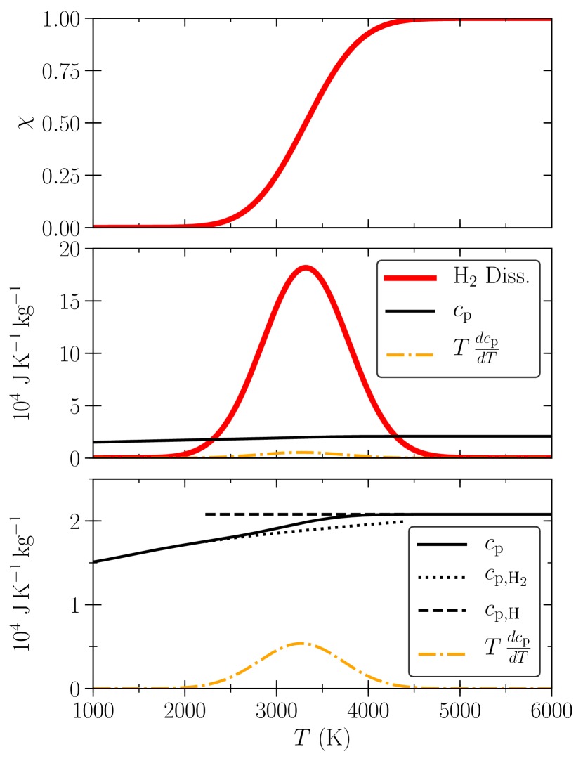
Figure 2: Top: The LTE dissociation fraction of H₂ in a parcel of gas. Middle: A demonstration of the relative importance of the H₂ dissociation/recombination term in Equation 8. For $2300\mathrel{\mathchoice{\raise 0.0pt\hbox{\scalebox{0.8}{\raise 0.0pt\hbox{$\displaystyle\lesssim$}}}}{\raise 0.0pt\hbox{\scalebox{0.8}{\raise 0.0pt\hbox{$\textstyle\lesssim$}}}}{\raise 0.0pt\hbox{\scalebox{0.8}{\raise 0.0pt\hbox{$\scriptstyle\lesssim$}}}}{\raise 0.0pt\hbox{\scalebox{0.8}{\raise 0.0pt\hbox{$\scriptscriptstyle\lesssim$}}}}}T\mathrel{\mathchoice{\raise 0.0pt\hbox{\scalebox{0.8}{\raise 0.0pt\hbox{$\displaystyle\lesssim$}}}}{\raise 0.0pt\hbox{\scalebox{0.8}{\raise 0.0pt\hbox{$\textstyle\lesssim$}}}}{\raise 0.0pt\hbox{\scalebox{0.8}{\raise 0.0pt\hbox{$\scriptstyle\lesssim$}}}}{\raise 0.0pt\hbox{\scalebox{0.8}{\raise 0.0pt\hbox{$\scriptscriptstyle\lesssim$}}}}}4300$, the energy absorbed by H₂ dissociation is greater than the energy stored as heat. Typical hot Jupiters are too cool to be affected by H₂ dissociation/recombination, but these processes should dominate on UHJs. Bottom: An inset showing the specific heat capacity of a gas composed of H and H₂ in LTE (the same black line from the middle panel), the specific heat capacities of H and H₂ where they are able to exist in equilibrium, and the additional $T(dc_{\rm p}/dT)$ term. All panels assume a pressure of 0.1 bar.

3 Simulated Observations and Qualitative Trends

We now explore the effects of this new term in the differential equation governing the temperature of a gas cell. For this purpose, we create a latitude+longitude HEALPix grid where each parcel’s temperature is updated using Equation 8 with code based on that developed by Schwartz et al. (2017).

While Cowan & Agol (2011) were able to explore their model using dimensionless quantities, our updated model requires that we use dimensioned variables. We therefore adopt the values of the first discovered UHJ, WASP-12b (Hebb et al., 2009). In particular, we set $R_{p}=1.90\,R_{J}$, $a=0.0234$ AU, $M_{p}=1.470\,M_{J}$, $T_{*,\text{eff}}=6360$ K, $R_{*}=1.657\,R_{\odot}$, $P=1.0914203$ days (Collins et al., 2017) and $A_{B}=0.27$ (Schwartz et al., 2017). We have also assumed a photospheric pressure of 0.1 bar, the approximate pressure probed by NIR observations of WASP-12b (Stevenson et al., 2014), which gives a radiative timescale of a few hours (similar to the observed timescales for eccentric hot Jupiters, e.g. Lewis et al., 2013; de Wit et al., 2016). Wind speeds for WASP-12b have not been directly measured, but typical values for hot Jupiters are on the order of 1 km s^-1 (e.g. Koll & Komacek, 2017); for that reason, we focus on wind speeds around this order of magnitude.

First, let’s explore the effects of H₂ dissociation/recombination at a spatially resolved scale. Figure 5 shows temperature and H₂ dissociation maps for three different wind speeds. In the limit of infinite wind speeds, there will be no temperature gradients and H₂ dissociation/recombination will not play a role. In the limit of an atmosphere in radiative equilibrium (wind speed = 0), there will be no variation in the temperature of a parcel and H₂ dissociation/recombination will play no role. Outside of these two unphysical limits, H₂ dissociation/recombination will always be occurring somewhere on UHJs.

Equatorial Zonal Wind Speeds

0.1 km s^-1

1.0 km s^-1

10 km s^-1

Temperature Maps

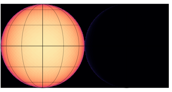
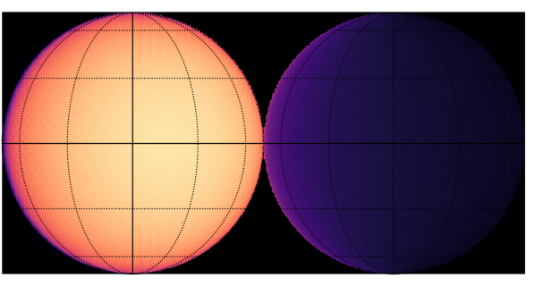
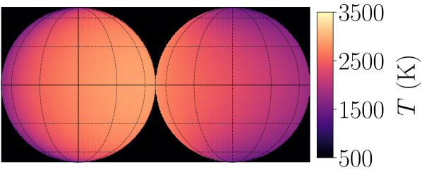
H₂ Dissociation Maps

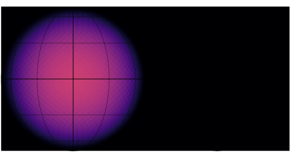
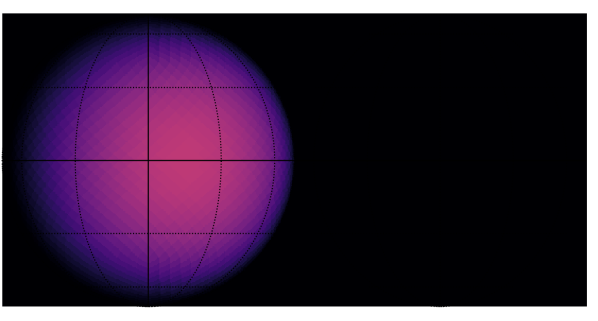
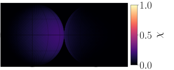
Figure 3: Planetary maps, showing temperature and H₂ dissociation fraction, assuming different eastward zonal wind speeds. The dayside hemisphere is shown on the left side of each map with north at the top.

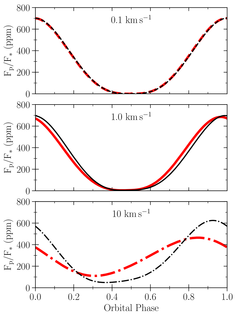
Figure 4: Model bolometric phasecurves assuming different eastward zonal wind velocities, ignoring eclipses and transits. The thick, red lines show the expected phasecurve accounting for H₂ dissociation/recombination, while the thinner, black models neglect these processes. Secondary eclipse would occur at a phase of 0.0, while a transit would occur at 0.5.

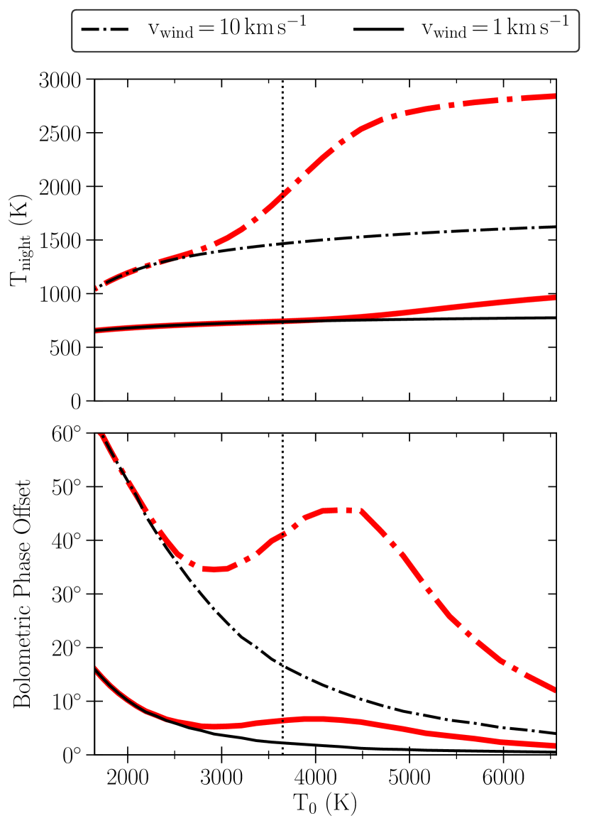
Figure 5: A figure showing the trends in nightside apparent temperature and phase offset as a function of irradiation temperature ($T_{0}\equiv T_{\rm*,eff}\sqrt{R_{*}/a}$), given theoretical bolometric phasecurve measurements. Thick, red lines show models including H₂ dissociation/recombination for WASP-12b, while thin, black lines show models neglecting these effects. Models sharing the same wind speed share linestyles, and all models assume a Bond albedo of 0.3 (which is typical for hot Jupiters; Zhang et al., 2018; Schwartz et al., 2017). A vertical dotted line shows the location of WASP-12b.

We now consider phasecurve observations — this requires that we convolve the planet map with a visibility kernel at each orbital phase (Cowan et al., 2013), which acts as a low-pass filter. Figure 5 shows model phasecurves for three wind speed; this figure shows that H₂ dissociation/recombination can have a significant effect. At a constant wind speed, the first obviously affected observable when accounting for dissociation/recombination is the increased offset of the peak in the phasecurve towards the east (the same direction as the prescribed wind). Another affected observable is the amplitude of the phase variations which is reduced when H₂ dissociation/recombination is included. Also, a Fourier decomposition shows that nearly all of the power in the phasecurves accounting for H₂ dissociation/recombination is in the first and second order Fourier series terms ($1f_{\text{orb}}$ and $2f_{\text{orb}}$). Finally, Figure 5 shows the trends in phase offset and nightside temperature for two wind speeds, both accounting for and neglecting H₂ dissociation/recombination.

4 Model Assumptions

With simplistic models, many important effects are necessarily swept under the rug. Here we aim to lift up the rug and shine a light on our assumptions to aid future work. While many of these assumptions will change the quantitative effects of H₂ dissociation/recombination, we expect that the overall qualitative impact of increased heat recirculation will be robust to these assumptions.

One important piece of physics that we have ignored (beyond a simple assumption of a 0.1 bar photosphere) is atmospheric opacity. As Dobbs-Dixon & Cowan (2017) demonstrated, variations in opacity sources as a function of longitude can change the depth of the photosphere by an order of magnitude or more. Changing the H₂ dissociation fraction will change the importance of H^- as an opacity source, and other standard opacity sources (e.g. H₂O and CO) will also likely be important, especially towards the cooler nightside. The insignificant detection of H₂O on the dayside of WASP-12b (Stevenson et al., 2014) but significant detection in the planet’s transmission spectrum (Kreidberg et al., 2015) clearly demonstrates that opacity sources should be expected to change on UHJs. Several of the standard molecular opacity sources will also overlap with the far broader H^- absorption, which complicates a definitive detection of H^- using broadband photometry, such as with Spitzer/IRAC. The formation of clouds on the nightside of the planet would further complicate the interpretation of observed phasecurves, increasing the albedo of the west terminator while also insulating the nightside. While we have accounted for variations in the radiative timescale as a function of temperature, we have not accounted for changes due to varying opacity sources.

Additionally, as we have assumed all photons are emitted at a 0.1 bar photosphere, the effects of the atmosphere’s T-P profile have been neglected. As the H₂ dissociation fraction has a fairly weak dependence on gas pressure, the bulk of vertical variations in the H₂ dissociation fraction will likely be controlled by the vertical temperature gradient. Due to the lower density of the dissociated gas, one may expect vertical advection on UHJs where temperature decreases with altitude. Interestingly, however, observations of most UHJs are best explained by atmospheres with thermal inversions (Arcangeli et al., 2018; Evans et al., 2017) or at least approximately isothermal profiles on the dayside (Crossfield et al., 2012; Cowan et al., 2012). Any non-isothermal T-P profile will alter the specifics of how efficiently heat is redistributed across the planet as different layers in a gas column will dissociate/recombine at different locations. Also, as we have neglected atmospheric opacity, we have assumed that each gas parcel emits as a blackbody with a single temperature.

Further, due to the changing scale height of the atmosphere at different latitudes and longitudes due to changes in temperature and H₂ dissociation fraction, there will likely be a tendency for gas to flow away from the sub-stellar point both zonally and meridionally. This is not accounted for in our toy model and would require a general circulation model. Instead, we have chosen eastward winds as they are predicted, and seen, for most hot Jupiters (e.g. Showman & Guillot, 2002; Zhang et al., 2018), although there are some exceptions (e.g. Dang et al., 2018). Similarly, our assumption of solid-body atmospheric rotation is clearly an over simplification which will need to be addressed in future work. Our model is also unable to predict the wind speeds of UHJs which would require the implementation of various drag sources, such as magnetic drag which Menou (2012) suggests will dominate at these high temperatures.

Also, we have assumed all heating is due to H₂ dissociation and radiation from the host star, neglecting other heat sources such as residual heat from formation (which should be negligible for planets older than 1 Gyr; Burrows et al., 2006) as well as tidal, viscous, and ohmic heating. We have also neglected the presence of helium which will partially dilute the strength of H₂ dissociation/recombination as only $\sim$80% of the atmosphere will be hydrogen. Finally, we have assumed that the planet has a uniform albedo which will not be the case in general (e.g. Esteves et al., 2013; Demory et al., 2013; Angerhausen et al., 2015; Parmentier et al., 2016).

5 Discussion and Conclusions

A new class of exoplanets is beginning to emerge: planets whose dayside atmospheres resemble stellar atmospheres as their molecular constituents thermally dissociate. The impacts of this dissociation will be varied and must be carefully accounted for. Here we have shown that the dynamical dissociation and recombination of H₂ will play an important role in the heat recirculation of ultra-hot Jupiters. In the atmospheres of ultra-hot Jupiters, significant H₂ dissociation occurs on the highly irradiated dayside, absorbing some of the incident stellar energy and transporting it towards the nightside of the planet where the gas recombines. Given a fixed wind speed, this will act to increase the heat recirculation efficiency; alternatively, a measured heat recirculation efficiency will require slower wind speeds once H₂ dissociation/recombination has been accounted for.

Both theoretically and observationally, it has been shown that increasing irradiation tends to lead to poorer heat recirculation (e.g. Komacek & Showman, 2016; Schwartz et al., 2017). However, there are a few notable exceptions to this rule at high temperatures. Recently, Zhang et al. (2018) reported a heat recirculation efficiency of $\varepsilon\sim 0.2$ for the UHJ WASP-33b which is far higher than would be predicted by theoretical and observational trends. WASP-12b may also possess an unusually high heat recirculation efficiency and exhibit a greater phase offset than would be expected from simple heat advection (Cowan et al., 2012). However, the power in the second order Fourier series terms from H₂ dissociation/recombination seems to make the phasecurve more sharply peaked and does not seem to be able to explain the double-peaked phasecurve seen for WASP-12b by Cowan et al. (2012). Also, while Arcangeli et al. (2018) find evidence of H₂ dissociation/recombination in the atmosphere of WASP-18b, Maxted et al. (2013) finds the planet has minimal day–night heat recirculation. Given the expected increase in heat recirculation due to H₂ dissociation/recombination, this suggests that WASP-18b has only moderate winds and/or is too cool for these processes to play a strong role in the heat recirculation of this planet. Finally, near-infrared observations of KELT-9b, the hottest UHJ currently known (Gaudi et al., 2017), could provide a fantastic test of this theory in the very high temperature regime.

References

- Amundsen et al. (2014) Amundsen, D. S., Baraffe, I., Tremblin, P., et al. 2014, A&A, 564, A59
- Angerhausen et al. (2015) Angerhausen, D., DeLarme, E., & Morse, J. A. 2015, PASP, 127, 1113
- Arcangeli et al. (2018) Arcangeli, J., Desert, J.-M., Line, M. R., et al. 2018, ArXiv e-prints, arXiv:1801.02489
- Bell et al. (2017) Bell, T. J., Nikolov, N., Cowan, N. B., et al. 2017, ApJ, 847, L2
- Berardo et al. (2017) Berardo, D., Cumming, A., & Marleau, G.-D. 2017, ApJ, 834, 149
- Burrows et al. (2006) Burrows, A., Sudarsky, D., & Hubeny, I. 2006, ApJ, 650, 1140
- Chase (1998) Chase, M. W. 1998, J. Phys. Chem. Ref. Data, Monograph 9, 1
- Collins et al. (2017) Collins, K. A., Kielkopf, J. F., & Stassun, K. G. 2017, AJ, 153, 78
- Cowan & Agol (2011) Cowan, N. B., & Agol, E. 2011, ApJ, 729, 54
- Cowan et al. (2013) Cowan, N. B., Fuentes, P. A., & Haggard, H. M. 2013, MNRAS, 434, 2465
- Cowan et al. (2012) Cowan, N. B., Machalek, P., Croll, B., et al. 2012, ApJ, 747, 82
- Crossfield et al. (2012) Crossfield, I. J. M., Barman, T., Hansen, B. M. S., Tanaka, I., & Kodama, T. 2012, ApJ, 760, 140
- Dang et al. (2018) Dang, L., Cowan, N. B., Schwartz, J. C., et al. 2018, ArXiv e-prints, arXiv:1801.06548
- de Wit et al. (2016) de Wit, J., Lewis, N. K., Langton, J., et al. 2016, ApJ, 820, L33
- Dean (1999) Dean, J. 1999, Lange’s handbook of chemistry, 36
- Demory et al. (2013) Demory, B.-O., de Wit, J., Lewis, N., et al. 2013, ApJ, 776, L25
- Dobbs-Dixon & Cowan (2017) Dobbs-Dixon, I., & Cowan, N. B. 2017, ApJ, 851, L26
- Esteves et al. (2013) Esteves, L. J., De Mooij, E. J. W., & Jayawardhana, R. 2013, ApJ, 772, 51
- Evans et al. (2017) Evans, T. M., Sing, D. K., Kataria, T., et al. 2017, Nature, 548, 58
- Gaudi et al. (2017) Gaudi, B. S., Stassun, K. G., Collins, K. A., et al. 2017, Nature, 546, 514
- Hebb et al. (2009) Hebb, L., Collier-Cameron, A., Loeillet, B., et al. 2009, ApJ, 693, 1920
- Heng & Kitzmann (2017) Heng, K., & Kitzmann, D. 2017, ApJS, 232, 20
- Hill (1986) Hill, T. L. 1986, An Introduction to Statistical Thermodynamics (Dover, New York)
- Koll & Komacek (2017) Koll, D. D. B., & Komacek, T. D. 2017, ArXiv e-prints, arXiv:1712.07643
- Komacek & Showman (2016) Komacek, T. D., & Showman, A. P. 2016, ApJ, 821, 16
- Kreidberg et al. (2015) Kreidberg, L., Line, M. R., Bean, J. L., et al. 2015, ApJ, 814, 66
- Lewis et al. (2013) Lewis, N. K., Knutson, H. A., Showman, A. P., et al. 2013, ApJ, 766, 95
- Maxted et al. (2013) Maxted, P. F. L., Anderson, D. R., Doyle, A. P., et al. 2013, MNRAS, 428, 2645
- Menou (2012) Menou, K. 2012, ApJ, 745, 138
- Parmentier et al. (2016) Parmentier, V., Fortney, J. J., Showman, A. P., Morley, C., & Marley, M. S. 2016, ApJ, 828, 22
- Perez-Becker & Showman (2013) Perez-Becker, D., & Showman, A. P. 2013, ApJ, 776, 134
- Pierrehumbert (2010) Pierrehumbert, R. T. 2010, Principles of Planetary Climate
- Rauscher & Menou (2010) Rauscher, E., & Menou, K. 2010, ApJ, 714, 1334
- Rink (1962) Rink, J. P. 1962, J. Chem. Phys., 36, 262
- Schwartz et al. (2017) Schwartz, J. C., Kashner, Z., Jovmir, D., & Cowan, N. B. 2017, ApJ, 850, 154
- Showman et al. (2009) Showman, A. P., Fortney, J. J., Lian, Y., et al. 2009, ApJ, 699, 564
- Showman & Guillot (2002) Showman, A. P., & Guillot, T. 2002, A&A, 385, 166
- Shui (1973) Shui, V. H. 1973, J. Chem. Phys., 58, 4868
- Stevenson et al. (2014) Stevenson, K. B., Bean, J. L., Madhusudhan, N., & Harrington, J. 2014, ApJ, 791, 36
- Zhang et al. (2018) Zhang, M., Knutson, H. A., Kataria, T., et al. 2018, AJ, 155, 83
- Zhang & Showman (2017) Zhang, X., & Showman, A. P. 2017, ApJ, 836, 73