Dark quarkonium formation in the early universe

Abstract

The relic abundance of heavy stable particles charged under a confining gauge group can be depleted by a second stage of annihilations near the deconfinement temperature. This proceeds via the formation of quarkonia-like states, in which the heavy pair subsequently annihilates. The size of the quarkonium formation cross section was the subject of some debate. We estimate this cross section in a simple toy model. The dominant process can be viewed as a rearrangement of the heavy and light quarks, leading to a geometric cross section of hadronic size. In contrast, processes in which only the heavy constituents are involved lead to mass-suppressed cross sections. These results apply to any scenario with bound states of sizes much larger than their inverse mass, such as U(1) models with charged particles of different masses, and can be used to construct ultra-heavy dark-matter models with masses above the naïve unitarity bound. They are also relevant for the cosmology of any stable colored relic.

1 Introduction

… and in the darkness bind them.

J. R. R. Tolkien

Stable “colored” particles, charged under QCD or a hidden confining gauge group, have been proposed as dark matter (DM) candidates Jacoby:2007nw ; Berger:2008ti ; Cheung:2008ke ; Chen:2009ab ; Davoudiasl:2010am ; Feng:2011ik ; Blinov:2012hq ; Bai:2013xga ; Cline:2013zca ; Boddy:2014yra ; Cline:2014kaa ; Boddy:2014qxa ; Forestell:2016qhc ; Harigaya:2016nlg ; Cline:2016nab ; Asadi:2016ybp ; Liew:2016hqo ; Cirelli:2016rnw ; Cline:2017tka ; Forestell:2017wov ; DeLuca:2018mzn ; Berlin:2018tvf , and are predicted in various extensions of the Standard Model Baer:1998pg ; Kang:2006yd ; Arvanitaki:2005fa . Even in the simplest models, the cosmological history of colored relics is intriguing, and their present-day abundances have been the subject of some debate. The relic abundance of a heavy colored particle $X$ is sensitive to the two inherent scales in the problem: its mass $m_{X}$, and the confinement scale $\Lambda_{D}$. If $m_{X}\gg\Lambda_{D}$, the freeze-out of $X$ proceeds via standard perturbative annihilations at temperatures $T\sim m_{X}/30$. However, at temperatures $T\sim\Lambda_{D}$, long after the perturbative $X$–$\bar{X}$ annihilations have shut off, the $X$ relic abundance may be further reduced by interactions of hadronized $X$s, whose size is set by $1/\Lambda_{D}$.

The annihilation process at $T\lesssim\Lambda_{D}$ was described in a semiclassical approximation in Ref. Kang:2006yd . At $T\sim\Lambda_{D}$, most of the $X$s are in color-singlet heavy-light hadrons, which we label by $H_{X}$. An $X$-hadron $H_{X}$ and an $\bar{X}$-hadron $\bar{H}_{X}$ experience a residual strong interaction whose effective range is $\sim 1/\Lambda_{D}$, much larger than the Compton wavelength $\sim 1/m_{X}$, but much smaller than the mean distance between $X$-hadrons at $T\sim\Lambda_{D}$. $X$–$\bar{X}$ annihilation then proceeds via the formation of $X$–$\bar{X}$ “quarkonia”, which subsequently de-excite to the ground state. In the ground state, the $X$–$\bar{X}$ distance is of order the Compton wavelength, and the pair annihilates into light mesons, (dark) photons, or glueballs. In the following, we use parentheses to denote quarkonium-like states, and refer to the $(X\bar{X})$ states as quarkonia.

The cross section for quarkonia formation was argued in Ref. Kang:2006yd to be purely geometric. This certainly holds for the scattering cross section of two $H_{X}$ hadrons; however, it is less clear that it holds for the quarkonium production cross section, which requires a significant modification of the trajectories of the heavy particles. One semiclassical argument for a mass-suppressed cross section was described in Ref. Arvanitaki:2005fa . To form a bound state, the $X$ and $\bar{X}$ must lose energy and angular momentum. Classically, one can estimate the cross section by modeling the energy loss as Larmor radiation. This is proportional to the acceleration-squared, which scales as $\Lambda_{D}^{4}/m_{X}^{2}$. At $T\sim\Lambda_{D}$, the $X$s are very slow, with speed $v\sim\sqrt{\Lambda_{D}/m_{X}}$. Thus it takes a long time for the hadrons to cross a distance $1/\Lambda_{D}$; however, the total amount of radiation still scales as $m_{X}^{-3/2}$ and is suppressed by the large $X$ mass.

Our goal in this paper is to quantify the cross section for dark quarkonia formation. This is, of course, a strong-coupling problem, so we will employ two simple toy models in which the calculation is tractable. As we will see, the results can be readily interpreted to infer the behavior of the cross section in the case of interest.

We consider a dark SU($N$) with two Dirac fermions $X$ and $q$ in the fundamental representation. We denote the SU($N$) confinement scale by $\Lambda_{D}$, although much of our discussion applies to real QCD as well. $X$ is heavy, with mass $m_{X}\gg\Lambda_{D}$, while $q$ is light, with $m_{q}\lesssim\Lambda_{D}$. We denote the color-singlet heavy-light mesons by $H_{X}\equiv X\bar{q}$ and $\bar{H}_{X}\equiv\bar{X}q$. The $X$ and $\bar{X}$, as well as their hadrons, are stable by virtue of a flavor symmetry.

We examine two prototypical contributions to quarkonia production in $H_{X}$–$\bar{H}_{X}$ collisions. The first is a radiation process, in which the “brown muck” is merely a spectator. To isolate the contribution of the heavy $X$s, we invoke a dark U(1), under which $X$ is charged while $q$ is neutral. The heavy fermions $X$ and $\bar{X}$ emit radiation in order to bind, and the relevant process is

$$H_{X}+\bar{H}_{X}\to(X\bar{X})+\varphi\qquad\text{[radiation by the $X$s]}.$$ (1)

Here $\varphi$ is the dark photon. Since the photon is emitted by the heavy $X$, the cross section for this process can be calculated using non-relativistic QCD (NRQCD) with a simple potential modeling the SU($N$) interaction. We use the Cornell potential, with a cutoff at a distance of order $1/\Lambda_{D}$ to simulate the screening by the brown muck. The resulting cross section is not geometric, but rather $m_{X}$-suppressed, in accordance with the simple semiclassical estimate above.

In the second process, the brown muck plays a key role in the interaction, leading to a geometric cross section for quarkonium formation. This happens, for example, when the radiation is emitted by the brown muck itself, which, as a result, exerts a force on the heavy $X$. While we cannot reliably calculate the cross section in this case, we can nonetheless capture the brown muck dynamics by considering the limit $m_{q}>\Lambda_{D}$, in which quarkonium formation can be thought of as a rearrangement of the heavy and light quarks,

$$\quad H_{X}+\bar{H}_{X}\to(X\bar{X})+(\bar{q}q)\qquad\text{[rearrangement]}.$$ (2)

The cross section for this process can be calculated in analogy with hydrogen-antihydrogen rearrangement into protonium and positronium. As we will see, for $m_{q}>\Lambda_{D}$, only the Coulombic states contribute. The result is a geometric cross section, which scales as the square of the Bohr radius $a_{q}=1/(\bar{\alpha}_{D}m_{q})$. Thus, quarkonium production is effective at low temperatures not because of confinement per se, but because of the large hierarchy between $a_{q}$ (the size of $H_{X}$) and $1/m_{X}$ (the Compton wavelength). We expect this result to persist as $m_{q}$ is dialed back below $\Lambda_{D}$: the quarkonium cross section will continue to scale as the size of $H_{X}$, which, in this case, is $1/\Lambda^{2}_{D}$.

As we will see, the geometric cross section arises from summing the contributions of many large (i.e., $\sim a_{q}$-sized) $X$–$\bar{X}$ bound states, for which the process is exothermic. These states cannot be dissociated, and will de-excite to the ground state, in which the $X$ and $\bar{X}$ annihilate. We will not discuss the cosmology of a specific model in detail, but merely sketch the essentials, following Ref. Kang:2006yd . Prior to the formation of the $H_{X}$ and $\bar{H}_{X}$ mesons, the $X$ particles annihilate and freeze out in the early universe with the standard relic density

$$\Omega^{\mathrm{ann}}_{X}h^{2}\sim\frac{10^{-9}\,\mathrm{GeV}^{-2}}{\left\langle\sigma^{\mathrm{ann}}_{X}v\right\rangle}\sim\left(\frac{m_{X}}{10^{4}\,\mathrm{GeV}}\right)^{2}\frac{1}{\alpha^{2}_{D}(m_{X})}\,.$$ (3)

Following the second stage of annihilations, the $H_{X}$ relic abundance is given by

$$\Omega^{f}_{H_{X}}\sim\sqrt{\frac{\Lambda_{D}}{m_{X}}}\,\left(\frac{m_{X}}{\text{30 TeV}}\right)^{2}\,.$$ (4)

Some fraction of $X$s remain in hadrons containing multiple $X$s, such as baryons. The various final abundances are model dependent and we do not explore them in detail here. Still, the late re-annihilations give a new mechanism for generating the relic abundance of dark matter, which is now a function of the two scales $m_{X}$ and $\Lambda_{D}$. This opens up many interesting directions to explore. We discuss some of the implications for cosmology in Sec. 5. In particular, the models can lead to a long era of matter domination between $m_{X}$ and $\Lambda_{D}$.

Note that the $X$s can hadronize with light quarks $q$, and the potential between them is screened at large distances. The cosmology of these models is thus somewhat different from quirky models. The presence of light quarks is important for yet another reason: even if there are no photons in the theory, energy loss can proceed via the emission of light pions. In contrast, in models with a pure SU($N$) at low energies, the lightest particles are glueballs, whose mass is $\sim 7\Lambda_{D}$.

The formalism and the results in this paper can be applied more broadly. For example, it is applicable to any confined heavy relic—be it all the dark matter or a component thereof, such as gluinos in split supersymmetry, messengers in gauge-mediated supersymmetry breaking, and so on.

This paper is structured as follows. The toy model is described in Sec. 2. The rearrangement calculation and its results are presented in Sec. 3. Section 4 focuses on the radiation process from the $X$s in which the brown muck is a spectator. In Sec. 5 we consider the dynamics of the $X$–$\bar{X}$ bound states generated by these processes and further implications for cosmology. In the Appendix, we collect some useful results on the properties of the Cornell and linear potentials and their wavefunctions, and discuss the details of the derivation of the cross section used in Sec. 4.

2 Description of the Toy Model

The minimal particle content in our models consists of two Dirac fermions, $(q,\bar{q})$ and $(X,\bar{X})$, in the fundamental representation of a dark SU($N$). In Sec. 4, we will assume that $X$ and $\bar{X}$ are also charged under a U(1) gauge symmetry. To describe the $X$–$\bar{X}$ interaction, we turn to models of quarkonium Novikov:1977dq ; Eichten:1978tg . The Cornell potential interpolates between the Coulombic QCD potential at small distances and the confining linear potential with string tension $\Lambda_{D}$ at large distances:

$$V_{\mathrm{Cornell}}(R)=-C\frac{\alpha_{D}}{R}+\Lambda^{2}_{D}R\,,$$ (5)

where $R$ is the distance between $X$ and $\bar{X}$, $C=(C_{1}+C_{2}-C_{12})/2$, and $C_{i}$ ($C_{12}$) are the quadratic Casimirs of the constituents (bound state). Since $X$ is a fundamental of SU($N$) and we require a color-singlet bound state, $C=C_{1}=C_{2}=(N^{2}-1)/(2N)$. The deep bound states of the system are then Coulombic, while the shallow states are controlled by the linear potential.

At large distances, the attractive potential is screened by the brown muck surrounding $X$ and $\bar{X}$. In QCD, for example, this distance is roughly the inverse of the string tension $\approx 400$ MeV (see, e.g., Refs. Brambilla:2004wf ; Brambilla:2010cs ). In order to capture this screening, the potential is cut off at a distance $R_{c}$,

$$V(R)=\begin{cases}-\bar{\alpha}_{D}\left(\frac{1}{R}-\frac{1}{R_{c}}\right)+\Lambda^{2}_{D}\left(R-R_{c}\right)\,+\,V_{0}&\text{for}\quad R<R_{c}\,,\\ V_{0}&\text{for}\quad R\geq R_{c}\,,\end{cases}$$ (6)

where $\bar{\alpha}_{D}=C\alpha_{D}$, and $V_{0}$ is a constant. The cutoff behavior will naturally emerge in the rearrangement calculation of Sec. 3, where we work in the calculable limit $m_{q}\gtrsim\Lambda_{D}$. For $m_{q}\gtrsim\Lambda_{D}$, the attractive potential is cut off at distances of order the Bohr radius of the heavy-light meson,

$$a_{q}=\frac{1}{\bar{\alpha}_{D}m_{q}}\,.$$ (7)

Thus, for $m_{q}$ sufficiently large, the problem reduces to a purely Coulombic potential, and we can calculate the cross section in analogy with hydrogen-antihydrogen rearrangement into protonium and positronium.

In Sec. 4 we will calculate quarkonia formation via radiation by the $X$s. Here the linear part of the potential is important, and the cutoff $R_{c}$ is introduced by hand. As we will describe, the choice of $R_{c}$ will be motivated by a comparison with the masses of $B$ and $D$ mesons in the Standard Model.

We note that, in QCD, the string tension in the confined phase and the dimensional transmutation scale from the running of the QCD gauge coupling are approximately the same Simolo:2006iw ; Brambilla:2010cs ; Patrignani:2016xqp , whereas the deconfinement temperature is about a factor of two lower Teper:2008yi . We will not be concerned with the lightest glueball state because its mass is a factor of about seven larger than the string tension Morningstar:1999rf .

3 The Rearrangement Process

At temperatures below $\Lambda_{D}$, the heavy $X$s are mostly found in $H_{X}$ ($X\bar{q}$) and $\bar{H}_{X}$ ($\bar{X}q$) mesons. These mesons can further deplete through $H_{X}$–$\bar{H}_{X}$ scattering into $(X\bar{X})$ quarkonia plus light hadrons. For $m_{q}<\Lambda_{D}$, the calculation of the cross section for this process requires the full machinery of perturbative NRQCD Brambilla:2004jw and is extremely difficult; we will limit ourselves to the case $m_{q}\gtrsim\Lambda_{D}$. This puts us firmly in the non-relativistic limit, in which quarkonium production can be thought of as rearrangement of the four partons,

$$H_{X}+\bar{H}_{X}\to(X\bar{X})+(q\bar{q}).$$ (8)

For $m_{X}\gg m_{q}$, the wavefunctions of the system can be calculated in the Born-Oppenheimer approximation, as in hydrogen-antihydrogen rearrangement into protonium and positronium HHbarcoll ; Jonsell:2001aa ; HHbarBO . We will closely follow this calculation, applying it to the near-threshold energies of interest.

If the semiclassical arguments in Ref. Kang:2006yd are correct, the cross section is expected to be geometric when the temperature is comparable to the binding energy of $H_{X}$, with no $m_{X}$ suppression. We verify this in the following calculation.

3.1 Setup

As discussed above, for $m_{q}$ sufficiently larger than $\Lambda_{D}$, only the Coulombic $(X\bar{X})$ states contribute. We will later comment on the validity of this approach as $m_{q}$ is taken below $\Lambda_{D}$.

The full interacting Hamiltonian of our system is written as the sum

$$\mathcal{H}_{\text{tot}}=\mathcal{H}_{\text{free}}+\mathcal{H}_{\text{int}}\,,$$ (9)

where

$$\mathcal{H}_{\text{free}} =-\frac{1}{m_{X}}\nabla^{2}_{R}-\frac{1}{2m_{q}}\nabla^{2}_{r_{q}}-\frac{1}{2m_{q}}\nabla^{2}_{r_{\bar{q}}}\,,$$

$$\mathcal{H}_{\text{int}} =V_{X\bar{X}}\left(R\right)+V_{q\bar{q}}\left(|{\bm{r}}_{q}-{\bm{r}}_{\bar{q}}|\right)+\mathcal{H}_{\text{tr}}\,,$$ (10)

$$\mathcal{H}_{\text{tr }} =V_{q\bar{X}}\left(|{\bm{r}}_{q}+{\bm{R}}/2|\right)+V_{\bar{q}X}\left(|{\bm{r}}_{\bar{q}}-{\bm{R}}/2|\right)-V_{\bar{q}\bar{X}}\left(|{\bm{r}}_{\bar{q}}+{\bm{R}}/2|\right)-V_{qX}\left(|{\bm{r}}_{q}-{\bm{R}}/2|\right)\,.$$

Here ${\bm{R}}$ is the vector from $\bar{X}$ to $X$ and ${\bm{r}}_{q},\,{\bm{r}}_{\bar{q}}$ are the positions of $q,\,\bar{q}$ relative to the $X$–$\bar{X}$ center-of-mass (CM), respectively, as shown in Fig. 1. The potentials $V_{q\bar{X}}$, $V_{\bar{q}X}$, $V_{qX}$, $V_{\bar{q}\bar{X}}$, $V_{q\bar{q}}$, and $V_{X\bar{X}}$ are the usual Coulomb potentials (with the relevant sign for same/opposite color quarks taken into account in Eq. (3.1)):

$$V(r)=-\frac{\bar{\alpha}_{D}}{r}\,.$$ (11)

Since we assume that $X$–$\bar{X}$ are in a color-singlet configuration, this factor is the same for the six potentials.

The calculation of the rearrangement cross section involves a subtlety well known to nuclear physicists: the asymptotic in and out states are not eigenstates of the same free Hamiltonian, but rather eigenstates of two different interacting Hamiltonians. This is different from conventional non-relativistic scattering where $\lim_{t\rightarrow\pm\infty}\mathcal{H}_{\text{tot}}=\mathcal{H}_{\text{free}}$. In our case, the infinite past Hamiltonian is

$$\mathcal{H}_{\text{in}}\equiv\lim_{t\rightarrow-\infty}\mathcal{H}_{\text{tot}}=\mathcal{H}_{\text{free}}+V_{q\bar{X}}\left(|{\bm{r}}_{q}+{\bm{R}}/2|\right)+V_{\bar{q}X}\left(|{\bm{r}}_{\bar{q}}-{\bm{R}}/2|\right)\,,$$ (12)

while the infinite future Hamiltonian is

$$\mathcal{H}_{\text{out}}\equiv\lim_{t\rightarrow\infty}\mathcal{H}_{\text{tot}}=\mathcal{H}_{\text{free}}+V_{X\bar{X}}\left(R\right)+V_{q\bar{q}}\left(|{\bm{r}}_{q}-{\bm{r}}_{\bar{q}}|\right)\,.$$ (13)

The scattering cross section is then calculated in the multi-channel formalism. By solving the Lippmann-Schwinger equation for multi-channel scattering (see, e.g., Ref. Taylor ), we get the simple formula for the cross section:

$$\frac{d\sigma}{d\Omega}=(2\pi)^{2}\frac{k_{f}}{k_{i}}m_{X}m_{q}|\mathcal{M}|^{2}\,,$$ (14)

where $k_{f}$ and $k_{i}$ are the momenta of the final and initial states in the CM frame (see below) and the transition matrix element is

$$\mathcal{M}=2\pi\Braket{\Psi_{f}({\bm{R}},{\bm{r}}_{q},{\bm{r}}_{\bar{q}})}{\mathcal{H}_{\text{tr}}}{\Psi_{i}({\bm{R}},{\bm{r}}_{q},{\bm{r}}_{\bar{q}})}\,,$$ (15)

where $\Psi_{f},\Psi_{i}$ are the final- and initial-state wavefunctions and $\mathcal{H}_{\text{tr}}=\mathcal{H}_{\text{tot}}-\mathcal{H}_{\text{out}}$, as can be seen from Eqs. (3.1) and (13). Note that in this representation of the cross section, the outgoing states $\Psi_{f}$ are eigenstates of $\mathcal{H}_{\text{out}}$, while the incoming states $\Psi_{i}$ are eigenstates of the full Hamiltonian $\mathcal{H}_{\text{tot}}$. Below, we discuss these states in more detail.

Figure 1: Coordinate system used in the calculation of the rearrangement process.

3.2 The incoming and outgoing wavefunctions

We wish to express our incoming and outgoing wavefunctions in the factorized form

$$\Psi({\bm{R}},{\bm{r}}_{q},{\bm{r}}_{\bar{q}})=\psi^{X\bar{X}}({\bm{R}})\,\psi^{q\bar{q}}(R;{\bm{r}}_{q},{\bm{r}}_{\bar{q}})\,.$$ (16)

In the final state this factorization is exact, since the outgoing $X$-onium and $q$-onium are asymptotically non-interacting. In other words:

$$\mathcal{H}_{\text{out}}=\mathcal{H}_{X\bar{X}}+\mathcal{H}_{q\bar{q}}\,,$$ (17)

with

$$\mathcal{H}_{X\bar{X}} =-\frac{1}{m_{X}}\nabla^{2}_{R}+V_{X\bar{X}}\left(R\right)\,,$$

$$\mathcal{H}_{q\bar{q}} =-\frac{1}{2m_{q}}\nabla^{2}_{r_{q}}-\frac{1}{2m_{q}}\nabla^{2}_{r_{\bar{q}}}+V_{q\bar{q}}\left(|{\bm{r}}_{q}-{\bm{r}}_{\bar{q}}|\right)\,.$$ (18)

The final state therefore trivially factorizes as the product of a plane wave for the outgoing $(q\bar{q})$ and the Coulomb bound states $\psi^{X\bar{X}}_{nlm}(R)$ (an eigenstate of $\mathcal{H}_{X\bar{X}}$) and $\psi^{q\bar{q}}_{100}({\bm{r}}_{q},{\bm{r}}_{\bar{q}})$ (an eigenstate of $\mathcal{H}_{q\bar{q}}$). For concreteness, we assume that the final-state $q$-onium is in its ground state and the $(X\bar{X})$ is static.

In contrast with the outgoing state, the incoming state is an eigenstate of the full Hamiltonian $\mathcal{H}_{\text{tot}}$, so we naïvely do not expect it to factorize as in Eq. (16). However, we can use the Born-Oppenheimer approximation to express it in this factorized form,

$$\Psi_{i}({\bm{R}},{\bm{r}}_{q},{\bm{r}}_{\bar{q}})=\psi^{X\bar{X}}_{i}({\bm{R}})\,\psi^{q\bar{q}}_{i}(R;{\bm{r}}_{q},{\bm{r}}_{\bar{q}})\,.$$ (19)

Since we are in the limit $m_{X}\gg m_{q}$, this is a very good approximation: at any given $X$–$\bar{X}$ distance $R$, $q$ and $\bar{q}$ will quickly adjust their configuration, and their wavefunction $\psi_{i}^{q\bar{q}}$ can therefore be calculated by integrating out $X$ and $\bar{X}$ and treating them as sources for the light quarks. This gives the energy and wavefunction of the light quarks for a fixed separation $R$ between the heavy $X$s as solutions to the eigenvalue problem

$$\left[\mathcal{H}_{\text{tot}}-\mathcal{H}_{X\bar{X}}\right]\psi^{q\bar{q}}_{i}=V_{\mathrm{BO}}({\bm{R}})\,\psi^{q\bar{q}}_{i}\,.$$ (20)

Substituting this back into the full Schrödinger equation and neglecting derivatives of $\psi^{q\bar{q}}_{i}$ with respect to the $X$–$\bar{X}$ coordinates, one obtains the equation for the $X$–$\bar{X}$ wavefunction,

$$\left[-\frac{1}{2m_{X}}\nabla^{2}_{R}+V_{X\bar{X}}(R)+V_{\mathrm{BO}}({\bm{R}})\right]\psi^{X\bar{X}}_{i}=E_{i}\,\psi^{X\bar{X}}_{i}\,.$$ (21)

Figure 2: The incoming effective potential $V_{\mathrm{in}}$ in units of $\bar{\alpha}_{D}^{2}m_{q}$ for the $X$–$\bar{X}$ system in the Born-Oppenheimer approximation (blue solid), as a function of $X$–$\bar{X}$ separation in units of the Bohr radius $a_{q}=1/(\bar{\alpha}_{D}m_{q})$. Also shown is the Coulomb potential for the $(X\bar{X})$ quarkonium (red dashed).

The effective potential for the $X$–$\bar{X}$ system is then

$$V_{\mathrm{in}}({\bm{R}})=V_{X\bar{X}}(R)+V_{\mathrm{BO}}({\bm{R}})$$ (22)

with

$$V_{\mathrm{BO}}({\bm{R}})=\Braket{\psi^{q\bar{q}}_{i}}{\mathcal{H}_{\text{tot}}-\mathcal{H}_{X\bar{X}}}{\psi^{q\bar{q}}_{i}}\,.$$ (23)

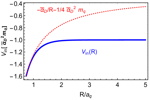
$V_{\mathrm{BO}}({\bm{R}})$ should interpolate between twice the binding energy of $H_{X}$, $2E_{b}\equiv\bar{\alpha}_{D}^{2}m_{q}$, at large $R$, and the $q$-onium binding energy, $-\bar{\alpha}_{D}^{2}m_{q}/4$, at small $R$. Unlike in molecules, for which the Coulombic repulsion of the nuclei must be overcome, here the two heavy particles attract each other, so we do not expect a significant potential barrier. These naïve expectations are borne out in the calculation of Ref. BOpotn . Since $V_{\mathrm{BO}}({\bm{R}})$ does not depend on the initial energy of the system or on the mass $m_{X}$, we can extract $V_{\mathrm{BO}}({\bm{R}})$ from Ref. BOpotn . We plot $V_{\mathrm{in}}$ in Fig. 2: as expected, the effects of the light quarks captured in $V_{\mathrm{BO}}({\bm{R}})$ set in for $R$ of order $a_{q}$. Their main effect is to screen the $X$–$\bar{X}$ interaction at large $R$; in practice, this happens for $R\sim 2a_{q}$.

Since $V_{\mathrm{in}}({\bm{R}})$ approaches a constant at large $R$, the $X$–$\bar{X}$ wavefunction at large distances ($R\geq 4a_{q}$) is the standard free-particle solution,

$$\Psi_{i}({\bm{R}},{\bm{r}}_{q},{\bm{r}}_{\bar{q}})\xrightarrow{R\geq 4a_{q}}\sum_{l}i^{l}\sqrt{2l+1}\,e^{i\delta_{l}}\left[\cos\delta_{l}\,j_{l}(k_{i}R)-\sin\delta_{l}\,n_{l}(k_{i}R)\right]Y_{l0}(\theta_{R})\psi^{q\bar{q}}_{i}({\bm{R}};{\bm{r}}_{q},{\bm{r}}_{\bar{q}})\,.$$ (24)

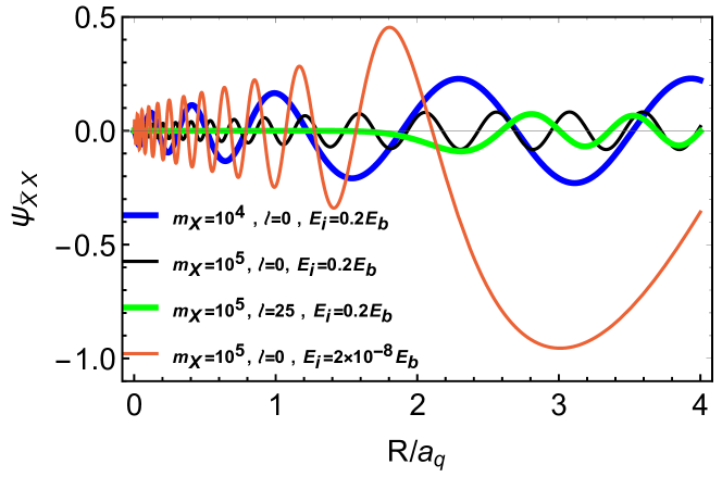
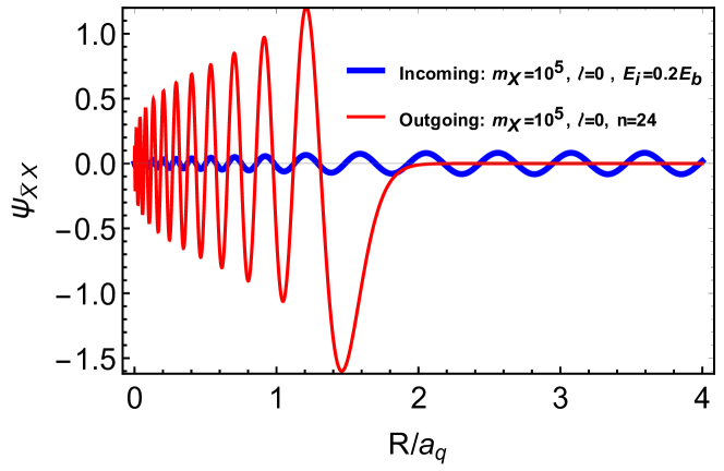
The wavefunctions for $R\leq 4a_{q}$ are found numerically, while their normalization is fixed by matching to Eq. (24) at $R=4a_{q}$. Some examples for the incoming and outgoing wavefunctions are given in Fig. 3.

Figure 3: Examples of incoming wavefunctions with various $m_{X},E_{i},l$ (top) and a comparison of an incoming and outgoing wavefunction (bottom). $m_{X}$ is given in units of the inverse Bohr radius $\bar{\alpha}_{D}m_{q}$ and $E_{b}=\frac{1}{2}\bar{\alpha}_{D}^{2}m_{q}$ is the $H_{X}$ binding energy.

3.3 The matrix element for rearrangement

Using the factorized incoming and outgoing wavefunctions, the transition matrix element Eq. (15) can be written in position space as

$$\mathcal{M}=\int d^{3}{\bm{R}}\,\psi^{X\bar{X}*}_{f}({\bm{R}})\,\psi^{X\bar{X}}_{i}({\bm{R}})\,T({\bm{R}})\,,$$ (25)

where

$$T({\bm{R}})=\int d^{3}{\bm{r}}_{q}\,d^{3}{\bm{r}}_{\bar{q}}\,\,\psi^{q\bar{q}*}_{f}({\bm{r}}_{q},{\bm{r}}_{\bar{q}})\,\mathcal{H}_{\text{tr}}\,\psi^{q\bar{q}}_{i}(R;{\bm{r}}_{q},{\bm{r}}_{\bar{q}})\,.$$ (26)

We will assume that the angular part of $T({\bm{R}})$ is constant. This is justified when the $(q\bar{q})$ is in the ground state, and in the short-distance approximation for the plane wave of the $(q\bar{q})$ relative to the $(X\bar{X})$. The second condition is broken when $k^{2}_{f}$ becomes large enough, where we expect an $\operatorname{\mathcal{O}}(1)$ correction. We neglect this correction in this work, since we are mostly interested in the parametric behavior of this process.

It is easy to see that $T(R)$ is appreciable only for $R$ of order $a_{q}$. For $R\gg a_{q}$, this can be seen by substituting $\mathcal{H}_{\text{tr}}=V_{\mathrm{BO}}({\bm{R}})-\mathcal{H}_{q\bar{q}}$ in Eq. (26). $\psi^{q\bar{q}}_{f}$ is an eigenfunction of $\mathcal{H}_{q\bar{q}}$, so one is left with the overlap integral of $\psi^{q\bar{q}}_{f}$ and the asymptotic $\psi^{q\bar{q}}_{i}$ at large $R$. These solve the same Hamiltonian with different eigenvalues: the former is a bound state and the latter is a continuum state. For small $R$, the initial- and final-state wavefunctions in the integrand do overlap, but $\mathcal{H}_{\text{tr}}$ tends to zero.

The full calculation of $T(R)$ is complicated. In fact, the Born-Oppenheimer approximation breaks down for $R\lesssim 0.74a_{q}$, where the $q$ and $\bar{q}$ are no longer bound to their respective $X$ (see, e.g., Ref. HHbarBO ). Still, we can use this approximation to get a rough estimate of the cross section. In particular, $T(R)$ is independent of the mass $m_{X}$ in the Born-Oppenheimer approximation, so we can extract $T(R)$ from Ref. HHbarBO . The result in the relevant range ($R\sim a_{q}$) can be parametrized as

$$T(R)=\begin{cases}\beta\left[E_{f}+\frac{1}{4}\bar{\alpha}_{D}^{2}m_{q}-V_{\mathrm{BO}}(R)\right]&\text{for}\quad R>0.74a_{q}\,,\\ 0&\text{for}\quad R\leq 0.74a_{q}\,,\end{cases}$$ (27)

where $E_{f}$ is the kinetic energy in the final state and $\beta$ is an $\operatorname{\mathcal{O}}(1)$ factor determined by matching to the hydrogen-antihydrogen results. Evidently, $T(R)$ depends on the binding energy of the $(X\bar{X})$ quarkonium, $E_{b}^{X\bar{X}}$, since $E_{f}=E_{i}+E_{b}^{X\bar{X}}-\frac{3}{4}\bar{\alpha}_{D}^{2}m_{q}$.

3.4 Rearrangement results

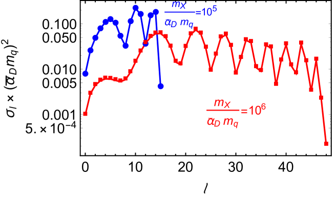
We calculate the cross section of Eq. (14) for different masses $m_{X}$ and incoming kinetic energies $E_{i}$, keeping $a_{q}$ fixed. In the approximation we use (see Sec. 3.3), the angular part of the overlap integral is translated into a selection rule $l_{X\bar{X}}=l_{i}\equiv l$. The breakdown of the cross section into partial waves—or $(X\bar{X})$ angular momenta—is given in Fig. 4 for high incoming kinetic energy $E_{i}=0.6E_{b}$ and $\bar{\alpha}_{D}=1/137$. We see that it vanishes above some maximal $l$, which corresponds to the classical angular momentum

$$l_{\mathrm{max}}\sim k_{i}a_{q}=\sqrt{E_{i}m_{X}}a_{q}\sim\sqrt{E_{i}m_{X}}/m_{q}\,.$$ (28)

Figure 4: The rearrangement cross section for each partial wave $l$, for two different values of $m_{X}$, with $E_{i}=0.6E_{b}$. All partial waves in the incoming state contribute up to a maximal $l\equiv l_{\mathrm{max}}\sim k_{i}a_{q}$.

It is also interesting to examine the branching fraction $\sigma_{nl}/\sigma_{l}$ for some initial partial wave to form an $(X\bar{X})$ quarkonium of definite binding energy. In Fig. 5 (left panel), we show this branching fraction for $l=0,14$, as a function of the final kinetic energy for two values of the initial kinetic energy $E_{i}/E_{b}=0.6,0.06$.

Figure 5: The branching fraction $\sigma_{nl}/\sigma_{l}$ for some initial partial waves to form an $(X\bar{X})$ quarkonium of definite $n,l$ (uniquely defined by the $x$-axis). The results are presented for $m_{X}=3\times 10^{4}\bar{\alpha}_{D}m_{q}$ and several values of $E_{i}$ and $l$. Left panel: The branching fraction as a function of the kinetic energy in the final state. Right panel: The branching fraction as a function of $R_{X\bar{X}}$, the mean radius of the final state.

Figure 6: The rearrangement cross section. The blue line is the total cross section for an incoming energy $E_{i}=0.6E_{b}$, and is geometric. Several individual partial-wave contributions ${\sigma_{l}}/{(2l+1)}$ are given in green, together with the unitarity bound $4\pi/k^{2}_{i}$ (red dashed line) for $l<l_{\mathrm{max}}\sim k_{i}a_{q}$.

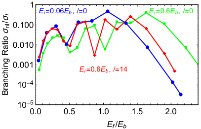
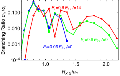
We see that quarkonium formation by rearrangement is an exothermic process: the kinetic energy in the final state does not vanish even when the initial momentum is taken to zero. Therefore the inverse process shuts off at low energies $\lesssim E_{b}$. Furthermore, only quarkonia with binding energies around $E_{b}$ are produced at $T\sim E_{b}$. The cross sections drop to zero for large final-state energies corresponding to $(X\bar{X}$) binding energies above $E_{b}$. Thus, deep Coulombic bound states with binding energies $E_{b}^{X\bar{X}}\sim\bar{\alpha}_{D}^{2}\,m_{X}$ are not formed in the rearrangement process. Correspondingly, the bound states produced are large, with size $\sim a_{q}$. This behavior is clearly exhibited in Fig. 5 (right panel), where we show the cross section as a function of the mean quarkonium radius $R_{X\bar{X}}$.

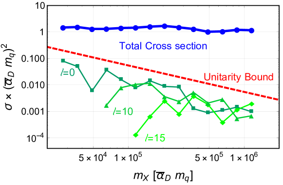
The total cross section for an initial energy of order the $H_{X}$ binding energy is plotted in Fig. 6 (blue line) as a function of $m_{X}$. Indeed, the cross section is geometric, $\sigma\sim a_{q}^{2}$, and is independent of $m_{X}$ to a very good approximation. It is interesting to compare the partial-wave contributions with the unitarity bound,

$$\sigma_{l}\leq(2l+1)\,\frac{4\pi}{k^{2}_{i}}\,.$$ (29)

We therefore also plot in this figure several individual partial-wave contributions normalized by $2l+1$ (green lines), compared to $4\pi/k^{2}_{i}$ (red dashed line). Clearly, for initial-state energies close to the binding energy of $H_{X}$, the cross section for each partial wave lies close to the unitarity bound. Summing over all the partial waves up to $l_{\mathrm{max}}$,

$$\sigma=\sum_{l=1}^{l_{\mathrm{max}}}\sigma_{l}\sim\frac{4\pi}{k^{2}_{i}}\sum_{l=1}^{l_{\mathrm{max}}}(2l+1)\sim\frac{4\pi}{k^{2}_{i}}l^{2}_{\mathrm{max}}\sim 4\pi a_{q}^{2}\,.$$ (30)

Thus the total cross section is geometric, and scales with the area of the $H_{X}$ bound state. In the low-temperature limit, we have checked that only $s$-wave processes are non-vanishing and the cross section scales as

$$\sigma\sim\frac{1}{k_{i}}a_{q}\,,$$ (31)

as demonstrated in Refs. HHbarcoll ; HHbarBO .

The above results apply to pure U(1) models. In the context of an SU($N$), we have explicitly seen that for $m_{q}$ above $\Lambda_{D}$, the light quarks truncate the $X$–$\bar{X}$ attraction for $R\gtrsim a_{q}$ via $V_{\mathrm{BO}}$, long before the linear potential sets in. This justifies neglecting the linear potential in the rearrangement calculation.

We can now turn to the limit of interest, $m_{q}$ below $\Lambda_{D}$. As we have seen above, the cross section scales with the size of the $H_{X}$ bound state, $a_{q}\gg 1/m_{X}$, thanks to the large number of partial waves contributing. This behavior is not special to the purely Coulombic case. In fact, the Coulombic contribution gives a conservative estimate of the cross section generated by the Cornell potential. Thus we expect a geometric cross section for $m_{q}$ below $\Lambda_{D}$, with the Bohr radius $a_{q}$ replaced by $1/\Lambda_{D}$.

The $X$–$\bar{X}$ bound states produced via rearrangement at $T\sim E_{b}$ are of size $\sim a_{q}$, much larger than the Compton wavelength of $X$. However, since the process is exothermic, these $X$–$\bar{X}$ bound states cannot be dissociated at $T\lesssim E_{b}$. In the case at hand, since there are light pions (or mesons) in the theory, nothing impedes the relaxation of these states to the ground state, in which the $X$–$\bar{X}$ pair annihilates.

4 The Radiation Process: Spectator Brown Muck

In the rearrangement process described above, the brown muck plays a central role. It is instructive to contrast this with a process in which the brown muck is merely a spectator. As we will see, in this case, the cross section scales with $m_{X}$.

To isolate the dynamics of the heavy quarks, we take $X$ to be charged under a dark U(1), while the light quarks are neutral. The relevant bound states are large, of size $\sim 1/\Lambda_{D}$, and are described by the linear part of the Cornell potential. To calculate $(X\bar{X})$ quarkonium production for $T\lesssim\Lambda_{D}$, we can therefore neglect the Coulombic part of the potential. This is also consistent with previous studies showing that, for pure U(1) models with no light charged particles, $(X\bar{X})$ bound-state formation gives only mild modifications of the $X$ relic abundance Feng:2009mn ; vonHarling:2014kha . For bound-state formation to deplete the $X$ abundance by orders of magnitude, a new scale is required. In the radiation process considered here, the new scale is $\Lambda_{D}$.

The radiative quarkonium production process is then

$$H_{X}+\bar{H}_{X}\to(X\bar{X})+\varphi\,,$$ (32)

where $\varphi$ is a (dark) photon that couples only to $X$; however, our results below apply more generally to other light particles which can be emitted by $X$. Unlike in the previous section, here the light quarks $q$ are relativistic.

We will follow the field-theoretic formalism for computing bound-state formation cross sections with long-range interactions detailed in Ref. Petraki:2015hla . Alternatively, these results can be obtained using the standard non-relativistic QM approach for calculating transition amplitudes, treating the photon as a classical field Wise:2014jva ; An:2016gad .

The first step is to derive the spectrum and two-particle wavefunctions that describe the bound and scattering states of the $X$–$\bar{X}$ system. While the light quarks do not actively participate in the radiation process, they screen the heavy $X$s at large distances. This is captured by the cutoff $R_{c}$ in the potential of Eq. (6), and leads to a continuum of $H_{X}$–$\bar{H}_{X}$ states with energies above the open $H_{X}$–$\bar{H}_{X}$-production threshold. Roughly speaking, the hadron mass is given by the sum of the heavy constituent masses, with each light quark or gluon contributing about $\Lambda_{D}$ to the mass. More precisely,

$$m_{H_{X}}=m_{X}+\kappa_{\Lambda_{D}}\Lambda_{D}+\operatorname{\mathcal{O}}(\Lambda^{2}_{D}/m_{X}^{2})\,,$$ (33)

where $\kappa_{\Lambda_{D}}$ is an $\operatorname{\mathcal{O}}(1)$ constant Manohar:2000 . The spectrum of bottom and charm mesons in QCD suggests $\kappa_{\Lambda_{D}}\Lambda_{D}\sim 600$ MeV, with $\Lambda_{D}\sim 400$ MeV, so in the following, we set $\kappa_{\Lambda_{D}}=1.5$. To estimate the cutoff $R_{c}$, we use the fact that the maximal $H_{X}$ binding energy, $E_{b}^{\mathrm{max}}$, coincides with the onset of the continuum,

$$2m_{X}+E_{b}^{\mathrm{max}}=2m_{H_{X}}\,.$$ (34)

Since the maximal bound state energy of the linear potential is

$$E_{b}^{\mathrm{max}}=\Lambda^{2}_{D}R_{c}+\frac{l(l+1)}{m_{X}R_{c}^{2}}\sim\Lambda^{2}_{D}R_{c}\,,$$ (35)

we set the cutoff to

$$R_{c}=\frac{2\kappa_{\Lambda_{D}}}{\Lambda_{D}}=\frac{3}{\Lambda_{D}}\,.$$ (36)

In summary, the potential we consider is

$$V(R)=\begin{cases}\Lambda^{2}_{D}\left(R-R_{c}\right)&\text{for}\quad R<R_{c}\,,\\ 0&\text{for}\quad R\geq R_{c}\,,\end{cases}$$ (37)

with $R_{c}$ given by Eq. (36) and $V_{0}$ of Eq. (6) chosen as zero for convenience. Defining

$$R_{0}\equiv\left(\frac{\Lambda_{D}}{m_{X}}\right)^{1/3}\frac{1}{\Lambda_{D}}\,,\qquad E_{0}\equiv\left(\frac{\Lambda_{D}}{m_{X}}\right)^{1/3}\Lambda_{D}\,,$$ (38)

which are the characteristic splittings in energy and size between successive states, the radial part of the wavefunction, $\chi_{ln}$, solves

$$-\chi_{ln}^{\prime\prime}(x)+V^{l}_{\text{eff}}(x)\,\chi_{ln}(x)=\epsilon_{ln}\chi_{ln}(x)\,,$$ (39)

where $x=R/R_{0}$, $\epsilon_{ln}={E_{ln}}/{E_{0}}$, and

$$V^{l}_{\mathrm{eff}}(x)=\frac{l(l+1)}{x^{2}}+x-x_{c}$$ (40)

with $x_{c}={R_{c}}/{R_{0}}$.

Using the semiclassical approximation, we can estimate the maximal angular momentum $l_{\mathrm{max}}$ of the bound states and the energy $\epsilon_{\mathrm{min}}$ of the lowest bound state with a given $l$. The lowest energy bound state for each $l$ classically corresponds to a minimum of the effective potential; the position $x^{l}_{\mathrm{min}}$ and the energy $V^{l}_{\mathrm{eff}}(x^{l}_{\mathrm{min}})$ of the minimum must satisfy $x^{l}_{\mathrm{min}}<x_{c}$ and $V^{l}_{\mathrm{eff}}(x^{l}_{\mathrm{min}})<0$, which result in

$$l_{\mathrm{max}}\simeq\sqrt{\frac{4x_{c}^{3}}{27}}\,,\qquad\epsilon_{\mathrm{min}}\simeq 3\left(\frac{l}{2}\right)^{2/3}-x_{c}\,.$$ (41)

In Appendix A.1, we collect some results for the effective potential and radial wavefunctions for various choices of the parameters.

4.1 Radiation results

The cross section for $H_{X}+\bar{H}_{X}\to(X\bar{X})_{lmn}+\varphi$ in the CM frame of the initial state is given by

$$v_{\text{rel}}\frac{d\sigma_{{\bm{k}}\to lmn}}{d\Omega}=\frac{|{\bm{P}}_{\varphi}|}{128\pi^{2}m^{3}_{X}}\left|\bm{\mathcal{M}}_{{\bm{k}}\to lmn}\right|^{2}\,,$$ (42)

where ${\bm{P}}_{\varphi}$ is the three-momentum of the radiated light state and, assuming that $\varphi$ is massless,

$$|{\bm{P}}_{\varphi}|=E_{k}-E_{ln}\,,$$ (43)

where $E_{k}$ is the kinetic energy of the initial state. We calculate this cross section in Appendix A. It is useful to write the cross section in terms of dimensionless quantities as

$$v_{\text{rel}}\,\sigma_{k\hat{{\bm{z}}}\to ln}=\sum_{m=-l}^{l}v_{\text{rel}}\,\sigma_{k\hat{{\bm{z}}}\to lmn}=\frac{2e_{X}^{2}}{m_{X}^{2}}\left(\frac{\Lambda_{D}}{m_{X}}\right)^{2/3}J_{k,ln}\,,$$ (44)

where $e_{X}$ is the U(1) charge of $X$, $\epsilon_{k}={E_{k}}/{E_{0}}$,

$$J_{k,ln}=(\epsilon_{k}-\epsilon_{ln})^{3}\left[(l+1)\left|I_{k,l+1\to ln}\right|^{2}+l\left|I_{k,l-1\to ln}\right|^{2}\right]\,,$$ (45)

and $I$ is the radial wavefunction overlap integral

$$I_{k,l\pm 1\to ln}=\int dx\,x\,\chi^{*}_{ln}(x)\,\chi_{k,l\pm 1}(x)\,.$$ (46)

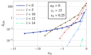
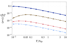
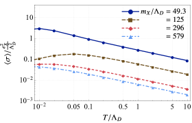
We plot $J_{k,ln}$ for several values of $l$ in Fig. 7, fixing $m_{X}/\Lambda_{D}=125$ and the initial kinetic energy $E_{k}/\Lambda_{D}=0.05$. As expected, the large, shallow bound states give the largest contributions.

Figure 7: $J_{k,ln}$ as a function of $\epsilon_{ln}$ for $x_{c}=15$ and $\epsilon_{k}=0.25$. The lines correspond to different values of $l$.

The total thermally-averaged cross section $\left\langle v_{\mathrm{rel}}\sigma\right\rangle$ (see Appendix A.3) is shown as a function of the temperature in Fig. 8 (left panel) for several choices of $m_{X}$. We also show $\left\langle\sigma\right\rangle$ for the same parameters (right panel). The cross section is clearly dependent on $m_{X}$, and decreases as $X$ becomes heavier. In fact, for $T\gtrsim 0.1\Lambda_{D}$, the scaling is well described by $\left\langle v_{\mathrm{rel}}\sigma\right\rangle\propto m_{X}^{-2}$ and $\left\langle\sigma\right\rangle\propto(m_{X}^{3}\Lambda_{D})^{-1/2}$, which agrees with the semiclassical estimate in Sec. 1. Thus, for the high mass region of interest, $m_{X}\gg\Lambda_{D}$, this contribution is negligible compared to processes mediated by the brown muck, such as the rearrangement process. We expect this qualitative behavior to persist regardless of the spin of the radiated particles.

Figure 8: Results of thermally-averaged radiative quarkonium production cross section $\left\langle\sigma v\right\rangle$ (left panel) and $\left\langle\sigma\right\rangle$ (right panel) as a function of temperature for different values of $m_{X}/\Lambda_{D}$.

5 Implications for Cosmology

We have found that, at temperatures below the confinement scale $\Lambda_{D}$, $(X\bar{X})$ bound states are formed with a geometric cross section with no $m_{X}$ suppression. These bound states are of size $\sim 1/\Lambda_{D}$, but since the process is exothermic, they cannot be dissociated, and eventually de-excite to the ground state, in which the $X$–$\bar{X}$ pair annihilates. The rate for this de-excitation process depends mainly on the light degrees of freedom. For the large $(X\bar{X})$ bound states produced, the level splittings are of order $(\Lambda_{D}/m_{X})^{1/3}\Lambda_{D}$, so we need massless photons or light pions in order to have allowed transitions (as in the models we considered here). In the case where the DM is charged under real QCD, the rate should be sizable, so we expect any $(X\bar{X})$ bound states to quickly decay to light particles.

As a result, the abundance of $H_{X}$ hadrons is depleted by this second stage of annihilations, down to Kang:2006yd

$$\Omega^{f}_{H_{X}}\sim\sqrt{\frac{\Lambda_{D}}{m_{X}}}\left(\frac{m_{X}}{\text{30 TeV}}\right)^{2}\,,$$ (47)

which can be much smaller than the relic density from perturbative $X$–$\bar{X}$ annihilations earlier in the thermal history.

There are, however, various different hadronic states (in addition to $H_{X}$) in which $X$ can survive Jacoby:2007nw . These include other types of single-$X$ hadrons such as baryonic $Xq^{N-1}$ hadrons, double-$X$ states such as baryonic $XXq^{N-2}$, and up to purely heavy baryons $X^{N}$. Thus, in general, our simple toy model can produce multi-component DM with different masses and relic abundances.

We leave a detailed investigation of the parameter space of the models for future study, but note a few qualitative features. The cross section for producing double-$X$ states should be comparable to the quarkonium cross section we calculated, albeit smaller by $\operatorname{\mathcal{O}}(1)$ factors because of the smaller binding energies in this case. However, for $N>2$, the double-$X$ hadrons contain some light quark(s), so their size is $1/\Lambda_{D}$. They can therefore interact quite efficiently with hadrons containing $\bar{X}$ to form bound states containing both $X$ and $\bar{X}$, where $X$–$\bar{X}$ pairs can quickly annihilate. Meanwhile, they can also interact with $H_{X}$ hadrons and form triple-$X$ hadrons, and this chain may go on until pure-$X$ (or pure-$\bar{X}$) baryons are formed. All these processes should have geometric cross sections. The pure-$X$ baryons eventually de-excite to the ground state, the size of which is much smaller than $1/\Lambda_{D}$. Their interactions with other hadrons therefore shut off. As a result, the $X$s inside the baryons remain as stable relics, while the other $X$s may effectively be annihilated. A systematic analysis necessitates solving the Boltzmann equation with these dynamics, which is beyond the scope of this work. However, it is safe to assume that a sizable fraction of the original $X$s can be preserved in a variety of stable hadronic relics.

For DM charged under real QCD, heavy-light hadrons, with size $1/\Lambda_{D}$, are subject to stringent constraints, but they are efficiently depleted at $T\lesssim\Lambda_{D}$ as we have shown. In contrast, the relic abundance of $X^{3}$ baryons may be just somewhat smaller than the original $X$ relic abundance. Thus the fundamental $X$s we considered here may give a different realization of colored DM DeLuca:2018mzn , but whether the models are viable requires a more detailed analysis. Note that the scenario considered in Ref. DeLuca:2018mzn , namely a heavy Dirac adjoint $X$, is non-generic, in that two $X$s can form a stable singlet with no additional light quarks.

In summary, the simple models considered here typically give rise to several components of DM composites of different masses. For certain choices of $m_{X}$ and $\Lambda_{D}$, these can exhibit self-interactions, transitions between different excited states, and, depending on the coupling to the Standard Model, modified direct and indirect detection cross sections. In some variants of these models, the DM abundance can be significantly depleted at $\Lambda_{D}$, leading to a long era of matter domination between $m_{X}$ and $\Lambda_{D}$.

6 Conclusions

In this paper we have considered the cosmological dynamics of bound states that are much larger than their inverse mass, taking as an example $X\bar{q}$ mesons in a confining theory where $X$ is much heavier than $q$ and the confinement scale. We calculated the cross section for quarkonium production from heavy-light meson scattering. The cross section is geometric, and scales with the area of the incident heavy-light mesons. The relic density of heavy-light $X$-mesons is therefore efficiently diluted with rates much higher than the $s$-wave unitarity bound due to the participation of many partial waves in the process. We also find that the process is mainly mediated by the effective interaction of the light quarks. In contrast, processes in which only the heavy constituents participate have mass-suppressed rates. It is amusing to note that if the lifetime of $B$-mesons were longer, such processes could be experimentally measured.

Appendix A Cross Section for Bound-State Formation in the Radiation Process

In this section we summarize the calculation of the bound-state formation cross section via radiation discussed in Sec. 4. We also collect here some useful results on the spectrum and wavefunctions of the Cornell and linear potential.

A.1 Eigenstates of the Cornell potential

We model the $X$–$\bar{X}$ attractive interaction by the cutoff Cornell potential of Eq. (6), with the cutoff given in Eq. (36) and $V_{0}=0$.

The bound states ($X\bar{X}$) are characterized by three integers $(l,m,n)$, where $l$ labels the angular momentum, $m$ labels the angular momentum along the $z$-axis, and $n\geq 1$. An $H_{X}$–$\bar{H}_{X}$ scattering state is approximated by an $X$–$\bar{X}$ unbound state, which is characterized by the $X$–$\bar{X}$ relative momentum ${\bm{k}}$, with energy $E_{k}\approx k^{2}/m_{X}$, where $k=|{\bm{k}}|$. The reduced mass of both the bound and scattering states is approximately $m_{X}/2$.

The bound-state wavefunctions can be written as

$$\psi_{lm,n}(R_{0}{\bm{x}})=\frac{1}{R_{0}^{3/2}}\frac{\chi_{ln}(x)}{x}Y_{lm}(\Omega_{\bm{x}})\,,$$ (48)

where the dimensionless coordinate $x$ is defined below Eq. (39). The scattering-state wavefunctions can be expanded as

$$\phi_{{\bm{k}}}(R_{0}{\bm{x}})=\sum_{l=0}^{\infty}(2l+1)\phi_{{\bm{k}},l}(R_{0}{\bm{x}})=\sum_{l=0}^{\infty}(2l+1)\frac{\chi_{kl}(x)}{x}P_{l}({\hat{{\bm{k}}}\cdot\hat{{\bm{x}}}})\,.$$ (49)

For ${\bm{k}}$ along $\hat{z}$ this simplifies to

$$\phi_{k\hat{\bm{z}},l}(R_{0}{\bm{x}})=\sqrt{\frac{4\pi}{2l+1}}\frac{\chi_{kl}(x)}{x}Y_{l}^{0}(\Omega_{\bm{x}})\,.$$ (50)

The radial wavefunctions $\chi_{ln}(x)$ and $\chi_{kl}(x)$ solve

$$-\chi^{\prime\prime}_{ln\,(kl)}(x)+V_{\mathrm{eff}}^{l}(x)\chi_{ln\,(kl)}(x)=\epsilon_{ln\,(k)}\chi_{ln\,(kl)}(x)\,,$$ (51)

where

$$\begin{split}V_{\mathrm{eff}}^{l}(x)&=\frac{l(l+1)}{x^{2}}+V(x)\\ &=\frac{l(l+1)}{x^{2}}+\left[{-a_{D}}\left(\frac{1}{x}-\frac{1}{x_{c}}\right)+\left(x-x_{c}\right)\right]\Theta(x_{c}-x)\,.\end{split}$$ (52)

Note that this dimensionless problem has only two parameters: $x_{c}$ and the effective Coulomb strength $a_{D}\equiv(m_{X}/\Lambda_{D})^{2/3}\bar{\alpha}_{D}$. The radial wavefunctions are zero at the origin, $\chi_{ln\,(kl)}(0)=0$, and satisfy the normalization conditions

$$\int_{0}^{\infty}\chi_{ln}(x)\chi^{*}_{ln^{\prime}}(x)dx=\delta_{nn^{\prime}}\,,\qquad\int_{0}^{\infty}\chi_{kl}(x)\chi^{*}_{k^{\prime}l}(x)dx=\frac{\pi}{2k^{2}}\delta(k-k^{\prime})\,,$$ (53)

so that $\braket{\psi_{lm,n}}{\psi_{l^{\prime}m^{\prime},n^{\prime}}}=\delta_{ll^{\prime}}\delta_{mm^{\prime}}\delta_{nn^{\prime}}$ and $\braket{\phi_{{\bm{k}}}}{\phi_{{\bm{k}}^{\prime}}}=(2\pi)^{3}\delta^{(3)}({\bm{k}}-{\bm{k}}^{\prime})$.

(a) $a_{D}=7$

(b) $a_{D}=0$ (linear)

Figure 9: The effective potential $V_{\mathrm{eff}}(x)$ with $x_{c}=15$ $(m_{X}\simeq 125\Lambda_{D})$, for three values of $l$. In the left figure, $a_{D}=7$, which corresponds to $\bar{\alpha}_{D}=0.3$, while $a_{D}=0$ in the right figure. The largest $l$ in each figure corresponds to the upper-bound on $l$ of the bound states. Note that the plots for $l=0$ correspond to $V(x)$ in Eq. (52).

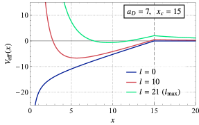
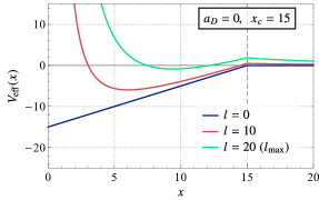
Figure 9 shows $V_{\mathrm{eff}}(x)$ in Eq. (52) for $x_{c}=15$ with $a_{D}=7$ (left) and $a_{D}=0$ (right). Because of the cutoff, the angular momentum quantum number $l$ of bound states has an upper bound $l_{\mathrm{max}}$ given in Eq. (41). This is confirmed in the numerical results.

(a) $a_{D}=7$

(b) $a_{D}=0$ (linear)

Figure 10: The energy spectrum of bound states. We also show, for the linear potential, the semiclassical results in Eq. (55) as the small dots.

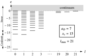
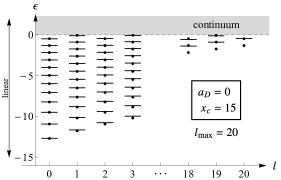
The bound-state energy levels are shown in Fig. 10 for a cutoff Cornell (left) and linear (right) potentials. In Ref. Quigg:1979vr , the semiclassical approximation is used to obtain the energy levels of the eigenstates of central potentials. Following their discussion, the energy levels under the linear potential are given by

$$E_{ln}-V(0)\approx\left[\frac{3}{2}\pi\left(n+\frac{l}{2}-\frac{1}{4}\right)\right]^{2/3}E_{0}\,,$$ (54)

or in our notation, since $V(0)=-R_{c}\Lambda^{2}_{D}=-x_{c}E_{0}$,

$$\epsilon_{ln}\approx\left[\frac{3}{2}\pi\left(n+\frac{l}{2}-\frac{1}{4}\right)\right]^{2/3}-x_{c}\,.$$ (55)

We reproduce this result in Fig. 10(b). For a Cornell potential (Fig. 10(a)), deep states are governed by the Coulomb force and therefore obey the well-known Coulombic energy levels

$$\epsilon_{ln}\approx-\frac{a_{D}^{2}}{4N^{2}}-x_{c}\,,$$ (56)

where the principal quantum number $N$ is given by $n+l$. For shallower states, the Coulomb force is negligible and the linear potential governs the spectrum.

Figure 11: Wavefunctions obtained from solving Eqs. (51–52) with $x_{c}=15,a_{D}=0$.
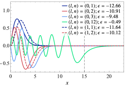
Top: $\chi_{ln}(x)$ for bound states. The left figure contains smaller $l$ (0,1) while the right figure has intermediate and high $l$ (5, 18, $19=l_{\mathrm{max}}$), where $(l,n)=(5,10)$ is the highest-energy bound state.
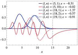
Bottom: $\chi_{kl}(x)$ for scattering states. The left figure displays the partial waves of the scattering states with $\epsilon=0.25$ ($E_{k}=0.05\Lambda_{D}$), while the right figure shows those with $\epsilon=7.5$ ($E_{k}=1.5\Lambda_{D}$).

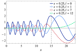
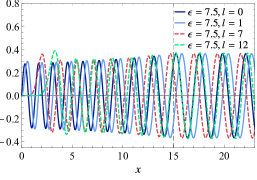
We show some examples of bound-state and scattering-state wavefunctions that solve Eq. (51) with the cutoff linear potential (Eq. (52) with $a_{D}=0$) in the top and bottom rows of Fig. 11, respectively. The bound state with $(l,n)=(5,10)$ is found to be the shallowest bound state, but it should be emphasized that this is an accident due to the cutoff being just above the energy of this state. In general, shallower states with smaller $l$ have wavefunctions that tend to penetrate beyond $x>x_{c}$. For the scattering states, wavefunctions of states with larger $\epsilon$ and smaller $l$ have penetrate further into the region $x<x_{c}$.

A.2 Bound-state formation cross section in the dipole approximation

We calculate the matrix element for the bound-state formation by a vector-mediated interaction,

$$H_{X}+\bar{H}_{X}\to(X\bar{X})_{lm,n}+\varphi$$ (57)

with the $X$–$\varphi$ interaction given by

$$\mathcal{L}\ni\left\lvert\left(\partial_{\mu}-ie_{X}\varphi_{\mu}\right)X\right\rvert^{2}\,.$$ (58)

We follow the approach and notation in Refs. Petraki:2015hla ; Petraki:2016cnz . From now on, we focus on the linear potential and set $a_{D}=0$ because, as we will see, the radiative bound-state formation process favors shallow bound states, for which the Coulomb force is negligible.

The bound-state formation cross section is given by Petraki:2015hla

$$(v_{\mathrm{rel}}\sigma)^{\mathrm{BSF}}_{{\bm{k}}}=\sum_{l,m,n}(v_{\mathrm{rel}}\sigma)^{\mathrm{BSF}}_{{\bm{k}}\to lm,n}=\sum_{l,m,n}\int\frac{d\Omega_{{\bm{P}}_{\varphi}}}{4\pi}\frac{|{\bm{P}}_{\varphi}|}{32\,\pi\,m^{3}_{X}}\sum_{\mathrm{pol.}}\left|{\bm{\epsilon}}\cdot\bm{\mathcal{M}}_{{\bm{k}}\to lm,n}\right|^{2}$$ (59)

in the CM frame, where ${\bm{k}}$, ${\bm{P}}_{\varphi}$, and ${\bm{\epsilon}}$ are the relative momentum of the initial state, the momentum of the radiated light state $\varphi$, and its polarization vector, respectively, and

$$v_{\mathrm{rel}}\simeq\frac{|{\bm{k}}|}{m_{X}/2}\,,\qquad|{\bm{P}}_{\varphi}|=E_{k}-E_{ln}\,;$$ (60)

$E_{k}$ is kinetic energy of the initial scattering state. The matrix element is

$$\mathcal{M}^{j}_{{\bm{k}}\to lm,n}=-4e_{X}\sqrt{m_{X}}\int\!\!\frac{d^{3}{\bm{p}}}{(2\pi)^{3}}\,p^{j}\tilde{\psi}_{lm,n}^{*}({\bm{p}})\left[\tilde{\phi}_{{\bm{k}}}\left({\bm{p}}+\frac{{\bm{P}}_{\varphi}}{2}\right)+\tilde{\phi}_{{\bm{k}}}\left({\bm{p}}-\frac{{\bm{P}}_{\varphi}}{2}\right)\right],$$ (61)

where $\tilde{\phi}_{{\bm{k}}}({\bm{p}})$ and $\tilde{\psi}_{lm,n}({\bm{p}})$ are the momentum-space equivalents of Eqs. (48)–(49).

It is convenient to expand the matrix element in partial waves (cf. Eq. (49)):

$$\mathcal{M}^{j}_{{\bm{k}}\to lm,n} =\sum_{l^{\prime}=0}^{\infty}(2l^{\prime}+1)\mathcal{M}^{j}_{{\bm{k}},l^{\prime}\to lm,n}\,,$$

$$\mathcal{M}^{j}_{{\bm{k}},l^{\prime}\to lm,n} =-4e_{X}\sqrt{m_{X}}\int\!\!\frac{d^{3}{\bm{p}}}{(2\pi)^{3}}\,p^{j}\tilde{\psi}_{lm,n}^{*}({\bm{p}})\left[\tilde{\phi}_{{\bm{k}},l^{\prime}}\left({\bm{p}}+\frac{{\bm{P}}_{\varphi}}{2}\right)+\tilde{\phi}_{{\bm{k}},l^{\prime}}\left({\bm{p}}-\frac{{\bm{P}}_{\varphi}}{2}\right)\right]$$

$$=8ie_{X}\sqrt{m_{X}}\int\!\!d^{3}{\bm{r}}\,d^{3}{\bm{r}}^{\prime}\,\psi^{*}_{lm,n}({\bm{r}})\phi_{{\bm{k}},l^{\prime}}({\bm{r}}^{\prime})\cos\left(\frac{{\bm{P}}_{\varphi}}{2}\cdot{\bm{r}}^{\prime}\right)\frac{\partial}{\partial r^{j}}\delta^{(3)}({\bm{r}}-{\bm{r}}^{\prime})\,.$$

After partial integration, the derivative acts on $\psi^{*}_{lm,n}({\bm{r}})$, and the integral over $d^{3}{\bm{r}}^{\prime}$ is trivial using the delta function. Dotting with the polarization vector and performing another partial integration (the derivative of the cosine is zero as $\bm{\epsilon}\cdot{\bm{P}}_{\varphi}=0$) yields

$${\bm{\epsilon}}\cdot{\bm{\mathcal{M}}}_{{\bm{k}},l^{\prime}\to lm,n}=4ie_{X}\sqrt{m_{X}}\int d^{3}{\bm{r}}\,\cos\left(\frac{{\bm{P}}_{\varphi}}{2}\cdot{\bm{r}}\right)\bm{\epsilon}\cdot\left[\psi^{*}_{lm,n}\bm{\nabla}\phi_{{\bm{k}},l^{\prime}}-\phi_{{\bm{k}},l^{\prime}}\bm{\nabla}\psi^{*}_{lm,n}\right]\,,$$ (62)

where $\psi^{*}_{lm,n}$ and $\phi_{{\bm{k}},l^{\prime}}$ are functions of ${\bm{r}}$. The quantity in brackets above appears in the difference of the Schrödinger equations for the scattering- and bound-state wavefunctions,

$$-\frac{1}{m_{X}}\bm{\nabla}\cdot(\psi^{*}_{lm,n}\bm{\nabla}\phi_{{\bm{k}},l^{\prime}}-\phi_{{\bm{k}},l^{\prime}}\bm{\nabla}\psi^{*}_{lm,n})=(E_{k}-E_{nl})\psi^{*}_{lm,n}\phi_{{\bm{k}},l^{\prime}}\,.$$ (63)

Using the identity

$$\int d^{3}{\bm{r}}\,\left({\nabla}\cdot{\bm{F}}\right){\bm{r}}=-\int d^{3}{\bm{r}}\,{\bm{F}}\left(\bm{\nabla}\cdot{\bm{r}}\right)=-\int d^{3}{\bm{r}}\,{\bm{F}}$$ (64)

with ${\bm{F}}=\psi^{*}_{lm,n}\bm{\nabla}\phi_{{\bm{k}},l^{\prime}}-\phi_{{\bm{k}},l^{\prime}}\bm{\nabla}\psi^{*}_{lm,n}$ and substituting into Eq. (62), we obtain

$$\begin{split}{\bm{\epsilon}}\cdot{\bm{\mathcal{M}}}_{{\bm{k}},l^{\prime}\to lm,n}=4ie_{X}\sqrt{m_{X}}&\int d^{3}{\bm{r}}\,({\bm{\epsilon}}\cdot{\bm{r}})\Bigg{[}m_{X}(E_{k}-E_{ln})\psi^{*}_{lm,n}\phi_{{\bm{k}},l^{\prime}}\cos\left(\frac{{\bm{P}}_{\varphi}}{2}\cdot{\bm{r}}\right)\\ &+\frac{{\bm{P}}_{\varphi}}{2}\cdot(\psi^{*}_{lm,n}\bm{\nabla}\phi_{{\bm{k}},l^{\prime}}-\phi_{{\bm{k}},l^{\prime}}\bm{\nabla}\psi^{*}_{lm,n})\sin\left(\frac{{\bm{P}}_{\varphi}}{2}\cdot{\bm{r}}\right)\Bigg{]}\,.\end{split}$$ (65)

We are interested in temperatures $T\lesssim\Lambda_{D}$ for which ${\bm{P}}_{\varphi}\ll m_{X}$, and thus

$${\bm{\epsilon}}\cdot{\bm{\mathcal{M}}}_{{\bm{k}},l^{\prime}\to lm,n}\simeq 4ie_{X}\sqrt{m_{X}^{3}}(E_{k}-E_{ln})\int d^{3}{\bm{r}}\,({\bm{\epsilon}}\cdot{\bm{r}})\psi^{*}_{lm,n}\phi_{{\bm{k}},l^{\prime}}\cos\left(\frac{{\bm{P}}_{\varphi}}{2}\cdot{\bm{r}}\right).$$ (66)

Also, we can evaluate ${\bm{P}}_{\varphi}\cdot{\bm{r}}/2$ as

$$\frac{{\bm{P}}_{\varphi}}{2}\cdot{\bm{r}}\leq\frac{|{\bm{P}}_{\varphi}|r}{2}=\frac{|E_{k}-E_{ln}|r}{2}=\kappa_{\Lambda_{D}}\frac{|E_{k}-E_{ln}|}{\Lambda_{D}}\frac{r}{R_{c}}\,.$$ (67)

Note that as the integrand contains a bound-state wavefunction, the integral has support only for $r\lesssim R_{c}$. Also, for $T\ll\Lambda_{D}$, the overlaps of the bound and scattering states are larger for shallower bound states. Combining these, we can approximate ${\bm{P}}_{\varphi}\cdot{\bm{r}}/2\ll 1$ in order to employ the dipole approximation $\cos({\bm{P}}_{\varphi}\cdot{\bm{r}}/2)\to 1$, which simplifies the cross section to

$$(v_{\mathrm{rel}}\sigma)^{\mathrm{BSF}}_{{\bm{k}}} \to\sum_{l,m,n}\int\frac{d\Omega_{{\bm{P}}_{\varphi}}}{4\pi}\frac{|{\bm{P}}_{\varphi}|}{32\,\pi\,m^{3}_{X}}\sum_{\mathrm{pol.}}\left|\sum_{l^{\prime}}(2l^{\prime}+1)4ie_{X}\sqrt{m_{X}^{3}}(E_{k}-E_{ln}){\bm{\epsilon}}\cdot{\bm{\mathcal{I}}}_{{\bm{k}},l^{\prime}\to lm,n}\right|^{2}$$

$$=\sum_{l,m,n}\int\frac{d\Omega_{{\bm{P}}_{\varphi}}}{4\pi}\frac{e_{X}^{2}(E_{k}-E_{ln})^{3}}{2\pi}\sum_{\mathrm{pol.}}\left|\sum_{l^{\prime}}(2l^{\prime}+1){\bm{\epsilon}}\cdot{\bm{\mathcal{I}}}_{{\bm{k}},l^{\prime}\to lm,n}\right|^{2},$$ (68)

where the integral of the wavefunctions is defined as

$$\begin{split}\mathcal{I}^{j}_{{\bm{k}},l^{\prime}\to lm,n}=\int d^{3}{\bm{r}}\,r^{j}\,\psi^{*}_{lm,n}\,\phi_{{\bm{k}},l^{\prime}}\,.\end{split}$$ (69)

Next, we express the integral in the basis $r^{a}=(r^{+},r^{0},r^{-})$ defined by

$$r^{\pm}=\frac{-1}{\sqrt{2}}\left(\pm r^{1}+ir^{2}\right)=r\,\sqrt{\frac{4\pi}{3}}\,Y^{\pm 1}_{1}\left(\Omega_{\bm{r}}\right)\,,\qquad r^{0}=r\,\sqrt{\frac{4\pi}{3}}\,Y^{0}_{1}\left(\Omega_{\bm{r}}\right)\,.$$ (70)

Taking the $z$-axis parallel to $\hat{\bm{k}}$, substituting Eq. (48) and Eq. (50) for the wavefunctions in Eq. (69), we obtain

$$\mathcal{I}^{a}_{{\bm{k}},l^{\prime}\to lm,n} =\frac{4\pi R_{0}^{5/2}}{\sqrt{3(2l^{\prime}+1)}}I_{kl^{\prime}\to ln}\int d\Omega_{\bm{x}}Y_{l^{\prime}}^{0}(\Omega_{\bm{x}})Y^{a}_{1}(\Omega_{\bm{x}})Y_{l}^{m*}(\Omega_{\bm{x}})$$

$$=(-1)^{m}\sqrt{{4\pi(2l+1)}}\,R_{0}^{5/2}I_{kl^{\prime}\to ln}\begin{pmatrix}l^{\prime}&1&l\\ 0&0&0\end{pmatrix}\begin{pmatrix}l^{\prime}&1&l\\ 0&a&-m\end{pmatrix},$$ (71)

$$I_{kl^{\prime}\to ln} =\int dx\,x\,\chi^{*}_{ln}(x)\,\chi_{kl^{\prime}}(x)\,,$$ (72)

where we have expressed the integral over solid angle of three spherical harmonics in terms of Wigner $3j$-symbols

$$\int d\Omega\,Y_{l_{1}}^{m_{1}}Y_{l_{2}}^{m_{2}}Y_{l_{3}}^{m_{3}}=\left[\frac{(2l_{1}+1)(2l_{2}+1)(2l_{3}+1)}{4\pi}\right]^{1/2}\begin{pmatrix}l_{1}&l_{2}&l_{3}\\ 0&0&0\end{pmatrix}\begin{pmatrix}l_{1}&l_{2}&l_{3}\\ m_{1}&m_{2}&m_{3}\end{pmatrix}\,.$$ (73)

These symbols give the selection rules $l^{\prime}=|l\pm 1|$ and $m=a$, so that $|m|\leq 1$.

With these results, the sum over $m,l^{\prime}$, and polarizations in Eq. (68) evaluates to

$$\sum_{m=-l}^{l}\sum_{\mathrm{pol.}}\left|\sum_{l^{\prime}}(2l^{\prime}+1){\bm{\epsilon}}\cdot{\bm{\mathcal{I}}}_{{\bm{k}},l^{\prime}\to lm,n}\right|^{2}$$

$$=\sum_{m=-l}^{l}\sum_{a=-1}^{1}\left|(2l+3){\mathcal{I}}^{m}_{{\bm{k}},l+1\to lm,n}+(2l-1){\mathcal{I}}^{m}_{{\bm{k}},l-1\to lm,n}\right|^{2}\delta_{am}$$

$$=\sum_{m=-1}^{1}\left|(2l+3){\mathcal{I}}^{m}_{{\bm{k}},l+1\to lm,n}+(2l-1){\mathcal{I}}^{m}_{{\bm{k}},l-1\to lm,n}\right|^{2}$$

$$=4\pi R_{0}^{5}\left[(l+1)\left|I_{k,l+1\to ln}\right|^{2}+l\left|I_{k,l-1\to ln}\right|^{2}\right].$$ (74)

Inserting this into the cross section in Eq. (68) and trivially performing the $d\Omega_{{\bm{P}}_{\varphi}}$ yields

$$(v_{\mathrm{rel}}\sigma)^{\mathrm{BSF}}_{{\bm{k}}} =2e_{X}^{2}R_{0}^{5}\sum_{l,n}(E_{k}-E_{ln})^{3}\left[(l+1)\left|I_{k,l+1\to ln}\right|^{2}+l\left|I_{k,l-1\to ln}\right|^{2}\right]$$

$$=\frac{2e_{X}^{2}}{m_{X}^{2}}\left(\frac{\Lambda_{D}}{m_{X}}\right)^{2/3}\sum_{l,n}J_{k,ln}\,,$$ (75)

with $J_{k,ln}$ defined in Eq. (45).

A.3 Thermally-averaged cross section

Here we briefly describe the procedure to calculate the thermally-averaged cross section, $\left\langle v_{\mathrm{rel}}\sigma\right\rangle(\beta)$, as a function of the inverse temperature $\beta=T^{-1}$. As in the previous discussion, we denote the momenta of the initial particles as ${\bm{k}}_{1}$, ${\bm{k}}_{2}$.

As we are interested in $T\ll m_{X}$, the kinetic distributions of $H_{X}$ and $\bar{H}_{X}$ are given by the Maxwell-Boltzmann distribution,

$$f_{\mathrm{MB}}({\bm{p}})=\left(\frac{2\pi\beta}{m}\right)^{3/2}\exp\left(-\frac{\beta|{\bm{p}}|^{2}}{2m_{X}}\right),$$ (76)

which is normalized so that $\int\!\!\frac{d^{3}{\bm{p}}}{(2\pi)^{3}}f_{\mathrm{MB}}({\bm{p}})=1$. With this distribution, the thermally-averaged cross section is given by

$$\left\langle v_{\mathrm{rel}}\sigma\right\rangle(\beta) =\int\!\!\frac{d^{3}{\bm{k}}_{1}}{(2\pi)^{3}}\frac{d^{3}{\bm{k}}_{2}}{(2\pi)^{3}}f_{\mathrm{MB}}({\bm{k}}_{1})f_{\mathrm{MB}}({\bm{k}}_{2})(v_{\mathrm{rel}}\sigma)^{\mathrm{BSF}}_{{\bm{k}}}$$

$$=\left(\frac{2\pi\beta}{m_{X}}\right)^{3}\int\!\!\frac{d^{3}{\bm{K}}}{(2\pi)^{3}}\frac{d^{3}{\bm{k}}}{(2\pi)^{3}}\exp\left(-\frac{\beta(|{\bm{K}}/2|^{2}+|{\bm{k}}|^{2})}{m_{X}}\right)(v_{\mathrm{rel}}\sigma)^{\mathrm{BSF}}_{{\bm{k}}}$$

$$=\sqrt{\frac{16\beta^{3}}{\pi m_{X}^{3}}}\int\!\!dk\,k^{2}\,e^{-\beta k^{2}/m_{X}}(v_{\mathrm{rel}}\sigma)^{\mathrm{BSF}}_{k}\,,$$ (77)

where, as before, ${\bm{K}}={\bm{k}}_{1}+{\bm{k}}_{2}$ and ${\bm{k}}=({\bm{k}}_{1}-{\bm{k}}_{2})/2$. We have neglected the dependence of the (non-relativistic) cross section $(v_{\mathrm{rel}}\sigma)^{\mathrm{BSF}}_{k}$ on ${\bm{K}}$ since $|{\bm{K}}|\ll|{\bm{k}}|$.

Combining the previous result and also including the final-state effect of $\varphi$, we obtain

$$\left\langle v_{\mathrm{rel}}\sigma\right\rangle(\beta)=\frac{2e_{X}^{2}}{m_{X}^{2}}\left(\frac{\Lambda_{D}}{m_{X}}\right)^{2/3}\int\!\!dk\,w(k;\beta)\sum_{l,n}\frac{J_{k,ln}}{1-\exp\left[-\beta(E_{k}-E_{ln})\right]}\,,$$ (78)

where we define

$$w(k;\beta)=\sqrt{\frac{16\beta^{3}}{\pi m_{X}^{3}}}\,k^{2}\,e^{-\beta k^{2}/m_{X}}\,,\qquad\int w(k;\beta)dk=1\,.$$ (79)

References

- (1) C. Jacoby and S. Nussinov, The Relic Abundance of Massive Colored Particles after a Late Hadronic Annihilation Stage. arXiv:0712.2681.
- (2) C. F. Berger, L. Covi, S. Kraml, and F. Palorini, The Number density of a charged relic, JCAP 0810 (2008) 005 [arXiv:0807.0211].
- (3) K. Cheung, W.-Y. Keung, and T.-C. Yuan, Phenomenology of iquarkonium, Nucl. Phys. B811 (2009) 274–287 [arXiv:0810.1524].
- (4) F. Chen, J. M. Cline, and A. R. Frey, Nonabelian dark matter: Models and constraints, Phys. Rev. D80 (2009) 083516 [arXiv:0907.4746].
- (5) H. Davoudiasl, D. E. Morrissey, K. Sigurdson, and S. Tulin, Hylogenesis: A Unified Origin for Baryonic Visible Matter and Antibaryonic Dark Matter, Phys. Rev. Lett. 105 (2010) 211304 [arXiv:1008.2399].
- (6) J. L. Feng and Y. Shadmi, WIMPless Dark Matter from Non-Abelian Hidden Sectors with Anomaly-Mediated Supersymmetry Breaking, Phys. Rev. D83 (2011) 095011 [arXiv:1102.0282].
- (7) N. Blinov, D. E. Morrissey, K. Sigurdson, and S. Tulin, Dark Matter Antibaryons from a Supersymmetric Hidden Sector, Phys. Rev. D86 (2012) 095021 [arXiv:1206.3304].
- (8) Y. Bai and P. Schwaller, Scale of dark QCD, Phys. Rev. D89 (2014) 063522 [arXiv:1306.4676].
- (9) J. M. Cline, Z. Liu, G. Moore, and W. Xue, Composite strongly interacting dark matter, Phys. Rev. D90 (2014) 015023 [arXiv:1312.3325].
- (10) K. K. Boddy, J. L. Feng, M. Kaplinghat, and T. M. P. Tait, Self-Interacting Dark Matter from a Non-Abelian Hidden Sector, Phys. Rev. D89 (2014) 115017 [arXiv:1402.3629].
- (11) J. M. Cline and A. R. Frey, Nonabelian dark matter models for 3.5 keV X-rays, JCAP 1410 (2014) 013 [arXiv:1408.0233].
- (12) K. K. Boddy, J. L. Feng, M. Kaplinghat, Y. Shadmi, and T. M. P. Tait, Strongly interacting dark matter: Self-interactions and keV lines, Phys. Rev. D90 (2014) 095016 [arXiv:1408.6532].
- (13) L. Forestell, D. E. Morrissey, and K. Sigurdson, Non-Abelian Dark Forces and the Relic Densities of Dark Glueballs, Phys. Rev. D95 (2017) 015032 [arXiv:1605.08048].
- (14) K. Harigaya, M. Ibe, K. Kaneta, W. Nakano, and M. Suzuki, Thermal Relic Dark Matter Beyond the Unitarity Limit, JHEP 08 (2016) 151 [arXiv:1606.00159].
- (15) J. M. Cline, W. Huang, and G. D. Moore, Challenges for models with composite states, Phys. Rev. D94 (2016) 055029 [arXiv:1607.07865].
- (16) P. Asadi, M. Baumgart, P. J. Fitzpatrick, E. Krupczak, and T. R. Slatyer, Capture and Decay of Electroweak WIMPonium, JCAP 1702 (2017) 005 [arXiv:1610.07617].
- (17) S. P. Liew and F. Luo, Effects of QCD bound states on dark matter relic abundance, JHEP 02 (2017) 091 [arXiv:1611.08133].
- (18) M. Cirelli, P. Panci, K. Petraki, F. Sala, and M. Taoso, Dark Matter’s secret liaisons: phenomenology of a dark U(1) sector with bound states, JCAP 1705 (2017) 036 [arXiv:1612.07295].
- (19) J. M. Cline, H. Liu, T. Slatyer, and W. Xue, Enabling Forbidden Dark Matter, Phys. Rev. D96 (2017) 083521 [arXiv:1702.07716].
- (20) L. Forestell, D. E. Morrissey, and K. Sigurdson, Cosmological Bounds on Non-Abelian Dark Forces. arXiv:1710.06447.
- (21) V. De Luca, A. Mitridate, M. Redi, J. Smirnov, and A. Strumia, Colored Dark Matter. arXiv:1801.01135.
- (22) A. Berlin, N. Blinov, S. Gori, P. Schuster, and N. Toro, Cosmology and Accelerator Tests of Strongly Interacting Dark Matter. arXiv:1801.05805.
- (23) H. Baer, K.-m. Cheung, and J. F. Gunion, A Heavy gluino as the lightest supersymmetric particle, Phys. Rev. D59 (1999) 075002 [hep-ph/9806361].
- (24) J. Kang, M. A. Luty, and S. Nasri, The Relic abundance of long-lived heavy colored particles, JHEP 09 (2008) 086 [hep-ph/0611322].
- (25) A. Arvanitaki, C. Davis, P. W. Graham, A. Pierce, and J. G. Wacker, Limits on split supersymmetry from gluino cosmology, Phys. Rev. D72 (2005) 075011 [hep-ph/0504210].
- (26) V. A. Novikov, et al., Charmonium and Gluons: Basic Experimental Facts and Theoretical Introduction, Phys. Rept. 41 (1978) 1–133.
- (27) E. Eichten, K. Gottfried, T. Kinoshita, K. D. Lane, and T.-M. Yan, Charmonium: The Model, Phys. Rev. D17 (1978) 3090 [Erratum ibid. D21 (1980) 313].
- (28) Quarkonium Working Group Collaboration, Heavy quarkonium physics. hep-ph/0412158.
- (29) N. Brambilla et al., Heavy quarkonium: progress, puzzles, and opportunities, Eur. Phys. J. C71 (2011) 1534 [arXiv:1010.5827].
- (30) N. Brambilla, M. A. Escobedo, J. Ghiglieri, and A. Vairo, Thermal width and gluo-dissociation of quarkonium in pNRQCD, JHEP 12 (2011) 116 [arXiv:1109.5826].
- (31) N. Brambilla, M. A. Escobedo, J. Ghiglieri, and A. Vairo, Thermal width and quarkonium dissociation by inelastic parton scattering, JHEP 05 (2013) 130 [arXiv:1303.6097].
- (32) C. Simolo, Extraction of characteristic constants in QCD with perturbative and nonperturbative methods. PhD thesis, Milan U., 2006. arXiv:0807.1501.
- (33) Particle Data Group Collaboration, Review of Particle Physics, Chin. Phys. C40 (2016) 100001.
- (34) M. Teper, Large N, PoS LATTICE2008 (2008) 022 [arXiv:0812.0085].
- (35) C. J. Morningstar and M. J. Peardon, The Glueball spectrum from an anisotropic lattice study, Phys. Rev. D60 (1999) 034509 [hep-lat/9901004].
- (36) N. Brambilla, A. Pineda, J. Soto, and A. Vairo, Effective field theories for heavy quarkonium, Rev. Mod. Phys. 77 (2005) 1423 [hep-ph/0410047].
- (37) P. Froelich, S. Jonsell, A. Saenz, B. Zygelman, and A. Dalgarno, Hydrogen-Antihydrogen Collisions, Phys. Rev. Lett. 84 (2000) 4577–4580.
- (38) S. Jonsell, A. Saenz, P. Froelich, B. Zygelman, and A. Dalgarno, Stability of hydrogen-antihydrogen mixtures at low energies, Phys. Rev. A 64 (2001) 052712.
- (39) S. Jonsell, A. Saenz, P. Froelich, B. Zygelman, and A. Dalgarno, Hydrogen–antihydrogen scattering in the Born–Oppenheimer approximation, J. Phys. B 37 (2004) 1195.
- (40) J. R. Taylor, Scattering Theory: The Quantum Theory on Nonrelativistic Collisions. John Wiley & Sons, Inc., 1972.
- (41) K. Strasburger, Accurate Born–Oppenheimer potential energy curve for the hydrogen–antihydrogen system, J. Phys. B 35 (2002) L435.
- (42) J. L. Feng, M. Kaplinghat, H. Tu, and H.-B. Yu, Hidden Charged Dark Matter, JCAP 0907 (2009) 004 [arXiv:0905.3039].
- (43) B. von Harling and K. Petraki, Bound-state formation for thermal relic dark matter and unitarity, JCAP 1412 (2014) 033 [arXiv:1407.7874].
- (44) K. Petraki, M. Postma, and M. Wiechers, Dark-matter bound states from Feynman diagrams, JHEP 06 (2015) 128 [arXiv:1505.00109].
- (45) M. B. Wise and Y. Zhang, Stable Bound States of Asymmetric Dark Matter, Phys. Rev. D90 (2014) 055030 [arXiv:1407.4121] [Erratum ibid. D91 (2015) 039907].
- (46) H. An, M. B. Wise, and Y. Zhang, Effects of Bound States on Dark Matter Annihilation, Phys. Rev. D93 (2016) 115020 [arXiv:1604.01776].
- (47) A. V. Manohar and M. B. Wise, Heavy quark physics, vol. 10 of Cambridge Monographs on Particle Physics, Nuclear Physics and Cosmology. Cambridge University Press, 2000.
- (48) C. Quigg and J. L. Rosner, Quantum Mechanics with Applications to Quarkonium, Phys. Rept. 56 (1979) 167–235.
- (49) K. Petraki, M. Postma, and J. de Vries, Radiative bound-state-formation cross-sections for dark matter interacting via a Yukawa potential, JHEP 04 (2017) 077 [arXiv:1611.01394].