Unlimited Accumulation of Electromagnetic Energy Using Time-Varying Reactive Elements
Abstract
Accumulation of energy by reactive elements is limited by the amplitude of time-harmonic external sources. In the steady-state regime, all incident power is fully reflected back to the source, and the stored energy does not increase in time, although the external source continuously supplies energy. Here, we show that this claim is not true if the reactive element is time-varying, and time-varying lossless loads of a transmission line or lossless metasurfaces can accumulate electromagnetic energy supplied by a time-harmonic source continuously in time without any theoretical limit. We analytically derive the required time dependence of the load reactance and show that it can be in principle realized as a series connection of mixers and filters. Furthermore, we prove that properly designing time-varying circuits one can arbitrarily engineer the time dependence of the current in the circuit fed by a given time-harmonic source. As an example, we theoretically demonstrate a circuit with a linearly increasing current through the inductor. Such circuits can accumulate huge energy from both the time-harmonic external source and the pump which works on varying the circuit elements in time. Finally, we discuss how this stored energy can be released in form of a time-compressed pulse.
I Introduction
Recently, time-space modulated structures attracted significant interest especially in realizing magnetless nonreciprocal devices. However, most of the studies have been limited to time-harmonic modulations, extending the classical results on mixers and parametric amplifiers. In this paper we look at new possibilities which can open up if we allow arbitrary time modulations of structure parameters (circuit reactances, material permittivity, etc). We expect that this approach may allow overcoming a number of important limitations inherent to conventional, harmonically modulated elements. As an interesting for applications example we consider capturing, accumulating, and storing of electromagnetic energy.
The use of conventional lossless reactive elements for energy accumulation is not efficient. Based on the circuit theory, we know that two fundamental reactive elements, the inductance and capacitance, store electromagnetic energy. If a time-varying current source is connected to an inductor , the stored magnetic energy equals . Replacing the inductor by a capacitor and employing a time-varying voltage source , we can store electric-field energy Jackson_book . Obviously, the stored energy is indeed limited by the source. To accumulate larger energy we need to have sources with larger output current or voltage. Even more importantly, most practically available sources whose energy we can harvest provide time-periodical (in particular, time-harmonic) output. In the case of time-harmonic sources (, where and represent the angular frequency and the amplitude, respectively), the stored energy is fluctuating between zero and (inductor fed by a current source) or (voltage-source fed capacitor). Therefore, the maximum amount of energy we can exploit is at , where ( denotes the period), and it is completely determined by the amplitude of the external source.
Now, the intriguing question which we consider here is if we can exceed this limitation for time-harmonic sources and continuously accumulate the energy supplied by the source in some reactive elements. The fundamental problem here is to eliminate reflections from a reactive load, so that all the incident power will be accumulated in the load and made available at some desired moment of time. If it is possible to control the time dependence of the external source, this problem can be solved by making the external voltage or current exponentially growing in time Baranov . Here, we are interested in more practical scenarios when the external source cannot be controlled (for instance, energy harvesting). Thus, we assume that the external source provides a given time-harmonic output and introduce solutions employing time-dependent reactive elements and/or . Note that the discussion here equally applies to circuits, waveguides, or waves incident on lossless boundaries, because in each of these cases the reflection and absorption phenomena can be modeled using an equivalent reactive load impedance.
Generally speaking, the use of time-varying elements in electronic circuits Cullen ; Fettweis ; Kamal ; Currie ; Baldwin ; Macdonald ; Anderson ; Liou ; Strom as well as time-varying material properties Slater ; Simon ; Hessel ; Holberg ; Gonzalez ; Biancalana ; Fan ; Sounas ; Fleury1 ; Fleury2 ; Alu (usually, time-varying permittivity) for engineering wave propagation have been attracting the researchers’ attention since approximately 1960s till today. These works are mainly focused on achieving nonreciprocity, amplification and frequency conversion. Here, we use time-varying reactive elements for energy accumulation. While in most of the earlier studies, periodical time variations of circuit elements have been used, for our goals we will need to consider arbitrary time variations of parametric elements.
The paper is organized as follows: In Section II, we apply the transmission-line theory and find the required condition to have zero reflection (unlimited accumulation of energy) in a line that is terminated by a single time-modulated reactive load. Subsequently, we elucidate our result by drawing an analogy between our time-modulated load and two different scenarios explained in the parts A and B of Section II, respectively. In Section III, we go one step further and consider a load which comprises two time-varying reactive elements that are in parallel with each other. In contrast to the case studied in Section II, here we show that it is possible to engineer the electric currents flowing through the elements while we still obtain zero reflection. We explain how engineering the electric currents affects the amount of energy accumulated by the entire load. Finally, Section IV concludes the paper. This paper is our first step that hopefully opens a way for further work on systems with arbitrary time modulations of parameters and, in particular, for practical investigations of efficient devices which accumulate energy from time-periodical, low-amplitude sources. We expect that the use of non-harmonic time modulations of system parameters will offer other, more general means to shape system response at will.
II Zero-reflection from time-modulated reactive elements
For a linear and time-invariant transmission line fed by a time-harmonic voltage/current source, the supplied energy is fully transferred to the load if the characteristic impedance of the line is equal to the load impedance of that line Pozar . Apparently, for the case of a lossless line terminated by a conventional inductance or capacitance, the energy is entirely reflected back as the incident wave arrives at the load, and therefore, there is no absorption nor accumulation of energy in the load. Mathematically, this property follows from the fact that the characteristic impedance of the line is real while the load impedance is purely imaginary (reactive).
It is easy to see that making the load reactance vary in time, it is possible to emulate resistance, although there is no actual power dissipation or generation. Indeed, the voltage over a capacitor/inductor and the current flowing through the element are related to each other as
| (1) |
where and denote the instantaneous voltage and current in a time-varying inductor or capacitor, respectively. Conventionally, when the element is time-independent, the second term in the above equations ( or ) vanishes and therefore, the voltage and current are proportional by a factor which is purely imaginary in the frequency domain. However, the scenario is completely different as the inductance/capacitance element varies with respect to time. The second term is not zero any more and it has the form of the usual Ohm law, where the role of the resistance or conductance is played by the time derivatives of the circuit reactances. Clearly, this virtual resistance or conductance describes virtual absorption of energy, which can be actually accumulated in the reactive element. Next, we will study how this possibility can be exploited for accepting and accumulating incident energy in reactive elements.
Let us consider a lossless transmission line loaded by a time-varying inductance and denote the voltage of the wave propagating towards the load as . The reflected voltage wave is denoted by . The instantaneous voltage over the load and the current flowing through the load are written as
| (2) |
where represents the characteristic impedance of the line. On the other hand, the voltage and the current are related to each other by Eq. (1). Substituting Eq. (1) into Eq. (2), we derive a general formula for the incoming and reflected waves at the load position as
| (3) |
In this equation, the left-hand side contains the terms measuring the reflected wave, while the right-hand side depends on the incident voltage only. For a given incident voltage and any time-dependent inductance we can find the reflected wave by solving the above first-order differential equation. Using Eq. (3) we can find ways to manipulate the reflected wave by choosing the proper function for . Here, we are interested in accumulating all the incident energy, that is, we are interested in reactive loads which do not reflect.
Now, assume that the incoming signal is time-harmonic, written as . In the following, the amplitude and the initial phase of the incident wave are supposed to be unity and zero, respectively, just for simplicity of formulas. Requiring absence of reflection (), we find the corresponding time dependence of from Eq. (3). Here, it is worth noting that the time-harmonic current in the load is in phase with the incident voltage in case of zero reflection, as is obvious from Eq. (2). The result reads
| (4) |
Such inductance as a load virtually absorbs all the input energy. Similar considerations can be made for loads in form of time-varying capacitance or other reactive loads. In the following, we explain the reason why the time-varying inductance described by Eq. (4) gives rise to the virtual absorption. To do this, we make an analogy between the inductance and a short-circuited line whose length is linearly increasing versus time. In addition, we also draw another analogy between the inductance and a load consisting of an infinite number of sinusoidal inductances connected in series.
II.1 Short circuited line
To understand the physical meaning of the result obtained above, we can notice a similarity of this formula (Eq. (4)) with the classical formula for the input reactance of a short-circuited transmission line:
| (5) |
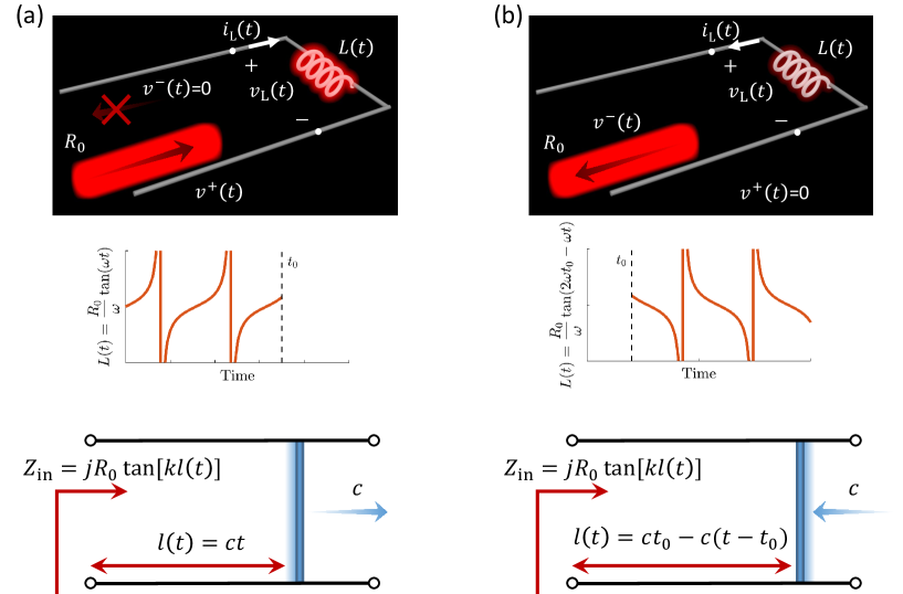
where ( denotes the phase velocity) is the phase constant and represents the length of the line. Obviously, the time-varying inductance given by (4) is the same as that seen at the input port of a lossless short-circuited transmission line if the length of the transmission line is linearly increasing with the constant velocity equal to , since in this case (see Fig. 1(a)). We see that in this conceptual scenario the reason for having no reflection from a lossless load is that the incident wave never reaches the reflecting termination, since the short is moving away from the input port with the same velocity as the phase front of the incident wave. Thus, varying the load inductance as prescribed by (4) for enough long time one can accumulate theoretically unlimited field energy in the reactive load.
Let us now assume that we would like to release the stored energy. To do that, we would reverse the direction of the velocity of the short, i.e. moving towards the input port (see Fig. 1(b)). All the energy stored in the line volume will be compressed in time and released into the feeding line at the moment when the length of the short circuited line becomes zero. The reactance of the line would correspond to a time-varying inductance given by
| (6) |
in which is the moment when the velocity of the short changes the direction and consequently, the short moves backward. Based on our analogy between the time-varying inductance and the short-circuited line whose length changes versus time, we conclude that the time-modulated inductance is expressed as
| (7) |
Here, and represent the time-modulated inductances in accumulation and releasing regimes, respectively. It is clear that the function describing is the mirror of the function describing with respect to the moment .
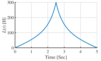
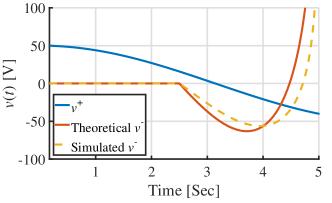
We have simulated the system illustrated by Fig. 1(a) (top one) utilizing MathWorks Simulink software. We assume that our system accumulates the energy till the moment s and subsequently, it releases the energy till the moment s. The modulation function for the reactive element expressed by Eq. (7) is shown in Fig. 2(a), and the simulated and theoretical results for the reflected wave are shown in Fig. 2(b). Notice that the theoretical formula for the reflected wave can be obtained using Eq. (3). The blue color in Fig. 2(b) corresponds to the incident wave [ V] while the red/yellow color represents the reflected wave. As it is seen, the reflection is zero till s meaning that the reactive element stores the electromagnetic energy (virtual absorption). After , the reflection appears and we are in the releasing regime. The theoretical and simulated results for the reflected wave are in good agreement.
Let us next consider the effects of inevitable dissipation losses in the system. Concentrating on the accumulating regime, we add a resistance () to the load in order to see the effect of ohmic losses. This load resistance is connected in series with the time-varying inductance. We have simulated again the structure in Fig. 1(a) and observed that if the load resistance is smaller than about % of the characteristic impedance of the transmission line (1 Ohm for our example of a 50-Ohm line), the reflected wave is still near zero and the system works quite well. For resistances larger than 1 Ohm (), some reflection appears and the efficiency decreases.
Interestingly, it is in fact possible to eliminate any reflections also for lossy terminations (with arbitrary values of ) by a simple modification of the modulation function of the time-varying inductance . This way we can compensate the resistive losses completely. Indeed, if we rewrite Eq. (3) by assuming that there is also the resistance at the termination, we see that the required time-varying inductance to obtain zero reflection becomes
| (8) |
According to the above expression, if , we will achieve the same result as given by Eqs. (4) or (7). Note that if , then the modulated inductance needed to eliminate reflections is zero because in this limiting case the load is already perfectly matched to the transmission line (perfect absorption condition). Our simulations have confirmed that the modification of the modulation function given by Eq. (8) indeed results in zero reflection in the accumulating regime for different values of loss resistance .
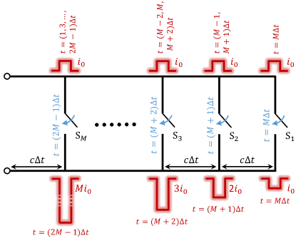
Similar effects of energy accumulation and release can be achieved using a transmission line periodically loaded with switches which can be switched at the appropriate time moments, as required by Eq. (5). Figure 3 schematically shows realization of this concept. Let us consider an incident signal in form of periodic pulses of amplitudes and durations . Prior to time moment , the pulses enter the transmission line and propagate along the line without any reflections because all the switches are open. When the first (leading) pulse approaches switch at time , it closes and the pulse reflects and starts propagating in the opposite direction. Due to the properly adjusted distance between the switches, at moment , the first pulse is summed up (constructive interference) with the second pulse which has been reflected by switch . The amplitude of the resulting pulse is doubled: . Likewise, at the position of each next switch the leading pulse amplitude is increased by , resulting in the output pulse with amplitude . In this scenario, the total energy entered the transmission line, proportional to , is compressed into a single pulse with energy . This is not a passive design since, due to the energy conservation, extra work proportional to is required for closing the switches.
II.2 Load consisting of sinusoidal inductances
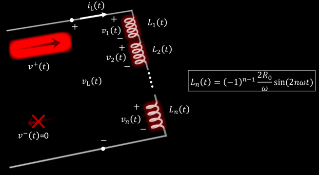
Another way to understand why the time-modulated inductance given by Eq. (4) ensures full virtual absorption is applying the Fourier series analysis. Since the required time-dependent load inductance given by Eq. (4) is a periodical function, we can expand it in the Fourier series. We know that
| (9) |
Using the above equation, we can consider the time-dependent inductance as an infinite collection of harmonically modulated inductances which are connected in series, as is illustrated in Fig. 4. Let us assume that the voltage over the whole load in the figure is and the current flowing through the load is . Based on the Kirchhoff voltage law, the voltage , where is the voltage over each time-dependent inductance. Therefore,
| (10) |
in which . Simplifying Eq. (10), we find that
| (11) |
Equation (11) shows that the th time-dependent inductance operates as a mixer in which the input of this mixer is a time-harmonic current signal of the frequency having the amplitude equal to producing as the output two time-harmonic voltage signals of frequencies and the amplitude of . The output signal can be amplified or attenuated depending on the integer number of the inductance element (it is amplified if ).
By substituting in Eq. (11), we realize that only the first harmonic corresponding to is not canceled in the series (which in the usual sense does not convergence). The second term of cancels out with the first term of , and the second term of is canceled by the first term of , and so on. Hence, only the first term of survives. Since the amplitude of this term is equal to the amplitude of the total voltage , the reflection coefficient equals zero. Here, it is worth mentioning that if we have a finite number of the time-dependent inductances shown in the figure, we can still emulate full absorption. From the above considerations we see that only the first harmonic and the harmonic remain. The other harmonics automatically vanish. Thus, to emulate full absorption, we only need to remove the harmonic by using a low-pass filter. If we do not filter this harmonic, certainly, the reflection is not zero.
III Time-dependent parallel circuit
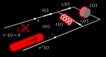
In the previous scenario with one reactive element, the electric current was limited by the characteristic impedance of the line and the amplitude of the incoming wave (). The intriguing question is if it is possible to realize any (growing) function for the electric current flowing through the time-varying reactive element. Next we will show that it is indeed possible if the time-varying reactive load contains at least two reactive elements, one inductive and one capacitive. Having two connected circuit elements we have an additional degree of freedom to shape the electric current flowing through these components since (assuming parallel connection) only the sum of the two currents should be equal to in order to ensure zero reflection. In this section we discuss the design of such circuits and investigate the stored energy in the system.
Let us consider a transmission line terminated by a parallel -circuit which is formed by time-dependent components and . Schematic of the circuit is illustrated by Fig. 5(a).
Suppose that the incident voltage wave is and the total electric current is (no reflection). Here, denotes the current through the inductance and denotes the current through the capacitance. Based on Kirchhoff’s current law, . This condition is fulfilled by setting the currents as
| (12) |
in which can be an arbitrary function of time. As an example, we consider as a linearly growing function in which (this is only due to the simplicity of the function, here any differentiable function can be assumed). Applying Kirchhoff’s laws and using Eq. (12), we can find the required time dependences of the circuit elements. After some algebraic manipulations, we obtain the following expressions:
| (13) |
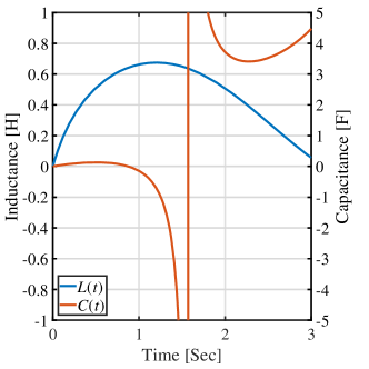
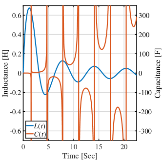
As the above equation shows, the capacitance always possess asymptotes due to the tangent function. However, depending on the ratio between and the angular frequency (), the inductance can be finite without having an asymptote. For example, Fig. 5(b) shows the functions of and for , rad/sec, V and A/sec. At the initial moment, both elements are positive and growing. However, later the inductance decreases and goes to zero fluctuating around it due to the term in the numerator.
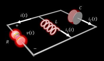
Modulating the elements in time as expressed in Eq. (13), no energy is reflected back to the source and all the input energy is continuously accumulated in the circuit. However, the reactances exchange energy also with the device which modulates their values in time. Thus, we need to consider the power balance and find how much energy is accumulated in the reactive circuit taking into account also the power exchange with the modulating system. To do this, we assume that the time modulation of the circuit elements stops at a certain time moment () and the circuit inductance and capacitance do not depend on time at later times . This means that at there is no power exchange with the system which modulates the reactances. At we connect a parallel resistance to the circuit as shown in Fig. 6(a), to form a usual circuit with time-invariant elements. We choose the moment at which the inductance and capacitance are both positive and calculate the energy delivered to the resistor during the relaxation time. This energy is equal to the energy which has been accumulated in the time-modulated circuit during the time . The rate of releasing the stored energy depends on the value of the resistance. If it is a small resistance, the accumulated energy is consumed in a short period of time. Let us choose as the moment when we stop modulation and energy accumulation. For the circuit in Fig. 6(a), we can write the second-order differential equation in form
| (14) |
Regarding the voltage over the elements, we know that . Solving the characteristic equation of the circuit, we obtain the electric current as
| (15) |
where
| (16) |
In Eq. (15), and are unknown coefficients which can be found by imposing the initial conditions, i.e. the current flowing through the inductance and the voltage over the capacitance should be continuous. In other words,
| (17) |
According to Eqs. (15) and (17), the coefficients and can be written as
| (18) |
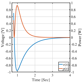
Knowing the electric current , we can calculate the resistance voltage and finally the instantaneous power as and the total released energy by integrating the instantaneous power from to infinity. This energy is the one that we can extract and use after stopping the modulation. Note that since at the values of and are such that and are real and not equal, the circuit is over-damped. The time dependence of the instantaneous power is shown in Fig. 6(b). We find that the energy consumed by the resistance is about J. Let us compare this value with the energy delivered to the matched circuit from the power source during the accumulation time from till , which equals J. Hence, the time-modulated load not only accumulated all the incident power but also accepted some power from the system which modulated the two reactances.
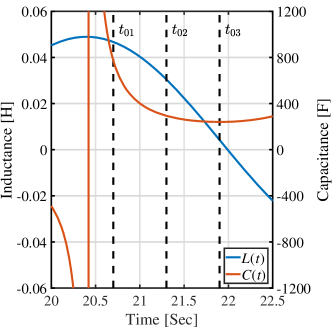
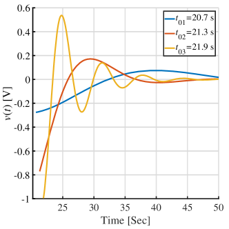
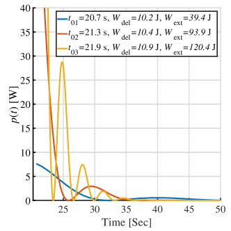
The above example with corresponds to a short energy-accumulation time. It is interesting to investigate energy accumulations for longer times. Figure 7 shows that near s, there is an asymptote for the capacitance function and the inductance is positive. Let us stop the reactance modulation at the following moments: s, s, and s, and connect a resistance to the time-invariant circuit at these moments. We choose such a small resistance value to release the accumulated energy quickly. Based on Eq. (16), because the value of the inductance is very small and the capacitance is very large, we expect that are complex and conjugate of one another: . In other words, the circuit is under-damped. This feature can be seen in Fig. 8 where we show the voltage over the resistance and the instantaneous power for the three different scenarios described above. Calculating the released energy, we find that while the delivered energy does not change much in these three cases ( and J), the energy which is accumulated and then extracted changes dramatically. It is worth noting that the extracted energy can be much larger than the delivered energy, showing that the modulated circuit accepts and accumulates energy also from the modulation source, in addition to the energy delivered by the source feeding the transmission line. However, stopping modulation and keeping and constant in time is only one way of extracting the energy. It is also possible to release the energy without stopping the modulation. We must only change the modulation function. Hence, we can choose a proper modulation function such that all the energy accepted by the circuit from the modulation source will return to the modulation source. In other words, an equal exchange of energy happens between the circuit and the modulation source in the accumulating and releasing regimes. In this scenario, the delivered energy becomes equal to the released (extracted) energy.
IV Conclusions
In this paper, we have shown that properly time-variant reactive elements can continuously accumulate energy from conventional external time-harmonic sources, without any reflections of the incident power. We have found the required time dependences of reactive elements and discussed possible realizations as time-space modulated transmission lines and mixer circuits. Interestingly, there is a conceptual analogy of energy-accumulating reactances and short-circuited transmission lines where the short position is moving, which helps to understand the physical mechanism of energy accumulation and release. We have shown that properly modulating reactances of two connected elements it is in principle possible to engineer any arbitrary time variations of currents induced by time-harmonic sources. The study of the energy balance has revealed that such parametric circuits accept and accumulate power not only from the main power source but also from the pump which modulates the reactances. This is seen from the fact that if we stop energy accumulation at some moment of time and release all the accumulated energy into a resistor, the released energy can be much larger than the energy delivered to the circuit from the primary source. These energy-accumulation properties become possible if the time variations of the reactive elements are not limited to periodical (usually time-harmonic) functions, but other, appropriate for desired performance, time variations are allowed.
Acknowledgement
The authors would like to thank Dr. Anu Lehtovuori for useful discussions on circuits with varying parameters.
References
- (1) J. D. Jackson, Classical Electrodynamics (John Wiley & Sons, New York, 1999).
- (2) D. G. Baranov, A. Krasnok and A. Alù, Coherent virtual absorption based on complex zero excitation for ideal light capturing, Optica 4, 1457 (2017).
- (3) A. L. Cullen, A travelling-wave parametric amplifier, Nature 181, 332 (1958).
- (4) A. Fettweis, Steady-state analysis of circuits containing a periodically-operated switch, IRE Trans. Circuit Theory 6, 252 (1959).
- (5) A. K. Kamal, A parametric device as a nonreciprocal element, Proceedings of the IRE 48, 1424 (1960).
- (6) M. R. Currie and R. W. Gould, Coupled-cavity traveling-wave parametric amplifiers: part I-analysis, Proceedings of the IRE 48, 1960 (1960).
- (7) L. D. Baldwin, Nonreciprocal parametric amplifier circuits, Proceedings of the IRE (Correspondence) 49, 1075 (1961).
- (8) J. R. Macdonald and D. E. Edmondson, Exact solution of a time-varying capacitance problem, Proceedings of the IRE 49, 453 (1961).
- (9) B. D. O. Anderson and R. W. Newcomb, On reciprocity and time-variable networks, Proceedings of the IEEE 53, 1674 (1965).
- (10) M. L. Liou, Exact analysis of linear circuits containing periodically operated switches with applications, IEEE Trans. Circuit Theory 19, 146 (1972).
- (11) T. Ström and S. Signell, Analysis of periodically switched linear circuits, IEEE Trans. Circuits Syst. 24, 531 (1977).
- (12) J. C. Slater, Interaction of waves in crystals, Rev. Mod. Phys. 30, 197 (1958).
- (13) J. C. Simon, Action of a progressive disturbance on a guided electromagnetic wave, IRE Trans. Microwave Theory Tech. 8, 18 (1960).
- (14) A. Hessel and A. A. Oliner, Wave propagation in a medium with a progressive sinusoidal disturbance, IRE Trans. Microwave Theory Tech. 9, 337 (1961).
- (15) D. E. Holberg and K. S. Kunz, Parametric properties of fields in a slab of time-varying permittivity, IEEE Trans. Antennas Propag. 14, 183 (1966).
- (16) J. R. Zurita-Sánchez, P. Halevi and J. C. Cervantes-González, Reflection and transmission of a wave incident on a slab with a time-periodic dielectric function , Phys. Rev. A 79, 053821 (2009).
- (17) F. Biancalana, A. Amann, A. V. Uskov and E. P. O’Reilly, Dynamics of light propagation in spatiotemporal dielectric structures, Phys. Rev. E 75, 046607 (2007).
- (18) K. Fang, Z. Yu and S. Fan, Photonic Aharonov-Bohm effect based on dynamic modulation, Phys. Rev. Lett. 108, 153901 (2012).
- (19) D. L. Sounas and A. Alù, Non-reciprocal photonics based on time modulation, Nature Photonics 11, 774 (2017).
- (20) T. T. Koutserimpas and R. Fleury, Nonreciprocal gain in non-Hermitian time-Floquet systems, Phys. Rev. Lett. 120, 087401 (2018).
- (21) T. T. Koutserimpas, A. Alù and R. Fleury, Parametric amplification and bidirectional invisibility in PT-symmetric time-Floquet systems, Phys. Rev. A 97, 013839 (2018).
- (22) R. Fleury, D. L. Sounas and A. Alù, Non-reciprocal optical mirrors based on spatio-temporal acousto-optic modulation, J. Opt. 20, 034007 (2018).
- (23) D. M. Pozar, Microwave Engineering (John Wiley & Sons, New Jersey, 2005).