Quantum Decoherence in System-Bath Interferometry

Abstract

In this paper, we study a quantum harmonic oscillator in a Mach-Zehnder-type interferometer which interacts with an environment, including electromagnetic oscillators. By solving the Lindblad master equation, we calculate the resulted interference pattern of the system. Interestingly, we show that even if one considers the decoherence effect, the system will keep some of its quantum properties. Indeed, the thermalization process does not completely leave the system in a classical state and the system keeps some of its coherency. Such an effect can be detected, when the frequency of the central system is high and the temperature is low, even with zero phase angle. This observation makes the quantum-to-classical transition remain as a vague notion in decoherence theory. By introducing an entropy measure, we express the influence of the bath as a maximization of system’s entropy instead of classicalization of the state.

I Introduction

Thermodynamics is a fundamental science of energy dissipation. Whenever a problem rises up in the borderlines of the physics, thermodynamics lies in the deepest layers of the problem. Thermodynamics is now applicable to describe a large variety of macroscopic systems, even in the order of cosmic scales Gold ; Liu . Yet, its description of systems in the quantum regime is blurred. In this regard, the question of how the thermodynamic rules apply in the microscopic scales is at the center of interests in recent works Gem ; Goo1 ; Vin . Furthermore, to assess if the properties of small numbers of microparticles could be described by the same macroscopic quantities, like entropy, broadly attracted the researchers into the field. For example, the equilibration experiments in atomic scales Trot , the introduction of new numerical methods for calculating of the thermodynamic properties Sch , and the study of the fundamental role of quantum information theory in the non-equilibrium statistical physics Jar ; Croo ; Pop ; del ; Bra , are among the recent works reported in this context.

The laws of equilibrium thermodynamics can be applied to classical closed systems and to open subsystems. There is a belief that these laws are also applicable to open quantum subsystems Nie . Decoherence theory makes it possible to study the thermodynamics of the open quantum systems. Moreover one of the interesting aspects of thermodynamics is its description of changes of a state through the decoherence. Many works with various perspectives have been done to study and define thermodynamic quantities for the open quantum systems by defining work, heat and thermodynamic laws in the quantum regime. This includes thermodynamics of discrete quantum processes And , the fluctuation theorems All ; Esp ; Tal , defining the passivity condition of the equilibrium state for the general quantum systems Pus and mathematical characterizations of these notions Hen ; Wei ; Deu ; Esp2 ; Esp3 ; Gem2 ; Wil ; San .

Although many works have been done to define thermodynamic quantities of interest in the quantum realm, especially the entropy, an appropriate setup is needed to study how these definitions work within the nature of the quantum processes. In this regard, there are interesting works which try to shed light on the subject, such as the violation of the Clausius inequality for a quantum harmonic oscillator linearly coupled to a bath of oscillatory fields All2 ; Hil , studying the distinction between the Gibbs-preserving maps and thermal operations Fai and the comparison of thermodynamic entropy of a quantum Brownian oscillator obtained by the partition function of the system with von Neumann entropy of the system Hor .

Nowadays it seems that the identity of the information is inseparable from its physical character. This makes an important role for quantum information in our understanding of quantum thermodynamics. Many thoughts emerge here to understand the fundamental relations between information and the statistical mechanics and thermodynamics . Accordingly, searching for thermodynamic rules in quantume regime is vastly quantum information oriented Gool . This includes entropy measures for quantifing the uncertainties about events Cov , emerging resource theories Fritz , equilibration and maximum entropy principle Lind ; Short , thermalization Riera and entanglement theory in thermodynamics Horo .

Here, we study the quantum second law of thermodynamics and the changes of entropy for a harmonic oscillator passing through a Mach-Zehnder-type interferometer, which coupled to a thermal bath. The idea is to study how the thermal bath affects the entropy and to see how it can change the interference pattern of the system. To do this, we use two convenient approaches. The first approach introduced by Binder and coworkers formulates an operational thermodynamics suitable for applying to an open quantum system undergoing a general quantum process, which can be described as a completely positive and trace-preserving (CPTP) map Bin . The other approach is based on the Clausius inequality with the definitions of work and heat as in Refs. Nie ; All2 .

The paper is organized as follows. In section II, we review the derivation of the master equation for a harmonic oscillator in a thermal bath consisting of electromagnetic oscillators, considering the conditions in which the Lindblad master equation holds. In section III, we briefly explain two common approaches on quantum thermodynamics used in this paper. In section IV, we solve the Lindblad master equation for a harmonic oscillator which enters a Mach-Zehnder-type interferometer, interacting with the thermal bath. Changes in the interference pattern are illustrated and the entropy variation is calculated. Finally, in section V, we discuss that how the system which is going through a thermalization process does not necessarily end up in a classical state. Also, by describing the role of the entropy in the process, quantum-to-classical transition concept of decoherence theory is revisited.

II Lindblad Model of Quantum Brownian Motion

The dynamics of the system here is discussed based on the Lindblad model of the quantum Brownian motion with the approach introduced by Maniscalco and coworkers Man . The Master equation first was introduced by Gorini, Kossakowski, and Sudarshan in which the Born-Markov approximation leads to a master equation in a Lindblad form known as GKSL (Gorini-Kossakowski-Sudarshan-Lindblad) equation Gori . In this system-reservoir model, the total Hamiltonian is defined by three parts

$$H=H_{s}+H_{\varepsilon}+H_{int},$$ (1)

where $H_{s}$,$H_{\varepsilon}$ and $H_{int}$ are respectively the system, the reservoir (environment) and the system-reservoir interaction Hamiltonians. The central system is a quantum harmonic oscillator and the environment is a thermal bath including electromagnetic oscillators. Therefore, the total Hamiltonian can be written as

$$H=(P^{2}+\Omega^{2}X^{2})/2+\sum_{i}(p_{i}^{2}+\omega_{i}^{2}q_{i}^{2})/2+H_{int},$$ (2)

where $\Omega$ ($\omega_{i}$) is the system (the environment) frequency and $P$ and $X$ ($p_{i}$ and $q_{i}$) are momentum and position operators of the system (the environment), respectively. For simplicity, we write off the mass and consider $\hbar=1$. The form of the interaction between the system and the environment is such that the position coordinate $X$ of the central particle couples linearly to the positions $q_{i}$ of the thermal bath oscillators with coupling strength $c_{i}$. Thus the interaction Hamiltonian $H_{int}$ reads

$$H_{int}=X\otimes E=X\otimes\sum_{i}c_{i}q_{i}.$$ (3)

Denoting $\rho$ as the total system-environment density matrix, the following assumptions are in order. First, the system and the environment are supposed to be uncorrelated at t=0 which means $\rho(0)=\rho_{s}(0)\otimes\rho_{\varepsilon}(0)$ with $\rho_{s}$ and $\rho_{\varepsilon}$ are the system and the environment density matrices, respectively. Second, we assume that the environment is stationary, that is $[H_{\varepsilon},\rho_{\varepsilon}(0)]=0$ and also the expectation value of $E$ is zero, $\text{Tr}_{E}[E\rho_{E}(0)]=0$. Finally, the system-environment coupling is weak and under the weak coupling, the factor of the oscillator frequency renormalization is negligible. Then, by averaging over the rapidly oscillating terms, one gets the following secular approximated master equation Man ; Bre

$$\frac{d\rho_{s}}{dt}= -\frac{\Delta(t)+\gamma(t)}{2}[a^{\dagger}a\rho_{s}-2a\rho_{s}a^{\dagger}+\rho_{s}a^{\dagger}a]$$

$$-\frac{\Delta(t)-\gamma(t)}{2}[aa^{\dagger}\rho_{s}-2a^{\dagger}\rho_{s}a+\rho_{s}aa^{\dagger}],$$ (4)

where $a=(X+iP)/\sqrt{2}$ and $a^{\dagger}=(X-iP)/\sqrt{2}$ are the bosonic annihilation and creation operators, respectively. Also, the time dependent coefficient $\gamma(t)$ is responsible for classical damping and $\Delta(t)$ is a diffusive term. These coefficients are defined as

$$\Delta(t) =\int_{0}^{t}\kappa(\tau)\cos(\Omega\tau)\text{d}\tau,$$ (5)

$$\gamma(t) =\int_{0}^{t}\mu(\tau)\sin(\Omega\tau)\text{d}\tau,$$ (6)

where

$$\kappa(\tau)=\sum_{i}c_{i}^{2}\langle\{q_{i}(\tau),q_{i}\}\rangle,$$ (7)

and

$$\mu(\tau)=i\sum_{i}c_{i}^{2}\langle[q_{i}(\tau),q_{i}]\rangle,$$ (8)

are noise and dissipation kernels, respectively.

The master equation (II) is similar to the Lindblad form but the coefficients are time-dependent. With the positive coefficients $\Delta(t)\pm\gamma(t)$ at all times, equation (II) is a Lindblad-type master equation Man2 . Let us consider the case of an Ohmic spectral density for the reservoir with Lorentz-Drude cutoff Schl

$$J(\omega)=\frac{2\gamma_{0}\omega}{\pi}\frac{\Lambda^{2}}{\Lambda^{2}+\omega^{2}},$$ (9)

where $\Lambda$ is the cut-off frequency and the dimensionless factor $\gamma_{0}$ describes the effective coupling strength between the system and the environment. Then, the coefficients $\Delta(t)$ and $\gamma(t)$ at the asymptotic long-time limit approach their stationary values, which their expression up to the second order in the coupling constant read as Man

$$\Delta =\gamma_{0}^{2}\Omega\frac{r^{2}}{1+r^{2}}\coth(\frac{\Omega}{2kT})$$ (10)

$$\gamma =\gamma_{0}^{2}\Omega\frac{r^{2}}{1+r^{2}},$$ (11)

where $k$ is Boltzmann constant, $T$ denotes temperature and $r=\Lambda/\Omega$. The master equation (II) becomes the well-known Markovian master equation of damped harmonic oscillator

$$\frac{d\rho_{s}}{dt}= -\Gamma(\bar{n}+1)[a^{\dagger}a\rho_{s}-2a\rho_{s}a^{\dagger}+\rho_{s}a^{\dagger}a]$$

$$-\Gamma\bar{n}[aa^{\dagger}\rho_{s}-2a^{\dagger}\rho_{s}a+\rho_{s}aa^{\dagger}],$$ (12)

where $\Gamma=\gamma_{0}^{2}\Omega r^{2}/(1+r^{2})$ and $\bar{n}=(e^{\Omega/kT}-1)^{-1}$. In this situation which the coefficients $\Delta\pm\gamma$ are positive, the aforementioned relation (II) is a Lindblad-type equation.

III Quantum Thermodynamic Program

The master equation (II) generates trace-preserving completely positive dynamics. Interestingly, the second law for CPTP map is known Bin ; Hat ; Sag . In quantum regime we consider von Neumann entropy $S(\rho)=-\text{tr}[\rho\log(\rho)]$ in the place of thermodynamic entropy which they are equal for thermal states. Therefore, the second law under the CPTP evolution becomes a consequence of the relative entropy, known as

$$S[\rho\parallel\sigma]=\text{tr}[\rho\log(\rho)-\rho\log(\sigma)],$$ (13)

in which, the relative entropy is finite when the intersection of $\text{ker}(\sigma)$ and $\text{supp}(\rho)$ is zero, obeying contractivity under CPTP maps Ved ; Lin

$$S[\rho\parallel\sigma]\geq S[M(\rho)\parallel M(\sigma)],$$ (14)

where $M(\rho)$ represents the density matrix $\rho$, undergoing a CPTP map $M$. When we study the changes of entropy $\Delta S=S[M(\rho)]-S(\rho)$, a reference state $\sigma$ is needed to be defined. The obvious and appropriate choice for the reference state is the map $M$ fixed point, i.e., $M(\xi)=\xi$. Then, the contractivity inequality (14) leads to the quantum version of Hatano-Sasa inequality Hat ; Sag

$$\Delta S\geq-\text{tr}[\{M(\rho)-\rho\}\log(\xi)]\text{.}$$ (15)

Individually, the quantum Hatano-Sasa inequality is valid for CPTP evolution, in which neither heat nor temperature is a well-defined quantity. However Binder et al. show that the second law of thermodynamics could be well-defined for the thermal maps Bin .

A map is thermal (also called Gibbs-preserving map), if it has a thermal state for its fixed point $\xi=\tau_{\beta}=\exp(-\beta\{H-F\})$ at temperature $\beta^{-1}$, where $F$ is its (Helmholtz) free energy Fai . Gibbs state $\tau_{\beta}$ is a stationary solution for the Lindblad-type master equation in the absence of external time-dependent fields Bre . Binder et al. show that for dephasing channels such as qubit dynamics governed by the master equation in Lindblad form, the Hatano-Sasa inequality (15) is written as Bin

$$\Delta S\geq 0.$$ (16)

In the second approach, on the other hand, the focus is on the Clausius inequalityNie ; All2 . Here, the internal energy $U$ is defined as stationary expectation value of the energy of the system

$$U=\langle H_{s}\rangle=\frac{\langle P^{2}\rangle}{2}+\frac{\Omega^{2}\langle X^{2}\rangle}{2}\text{.}$$ (17)

A quasistatic variation of $U$ can be written as

$$dU= \int\int\text{d}\mathcal{X}\text{d}\mathcal{P}W(\mathcal{X},\mathcal{P})\text{d}H_{s}(\mathcal{X},\mathcal{P})$$ (18)

$$+ \int\int\text{d}\mathcal{X}\text{d}\mathcal{P}H_{s}(\mathcal{X},\mathcal{P})\text{d}W(\mathcal{X},\mathcal{P}),$$

where $W(\mathcal{X},\mathcal{P})$ is Wigner distribution function for the system in the position-momentum space. The first term in the right-hand side is known as work $\delta W$ done on the system and the second term is known as heat $\delta Q$ exchanged with the bath. Since the Hamiltonian (2) is time-independent, the term identified as work is zero. Then, according to (17) the change in heat is

$$\delta Q=(\frac{\Omega^{2}}{2}\frac{\partial\langle X^{2}\rangle}{\partial t}+\frac{1}{2}\frac{\partial\langle P^{2}\rangle}{\partial t})\text{d}t.$$ (19)

In this approach, the entropy in the Clausius inequality is the same as the von Neumann entropy.

IV An Interferometer Coupled to a Thermal Bath

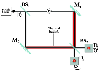
Figure 1: A particle in the state $|1\rangle$ enters the interferometer through the $50$:$50$ beamsplitter $BS_{1}$. After passing the Mirrors $M_{1}$ or $M_{2}$, it interacts with the thermal bath, affected by the decoherence process. Then by passing through the $50$:$50$ beamsplitter $BS_{2}$ it reaches the detectors $D_{1}$ or $D_{2}$.

Now we study a two-state ($|0\rangle$ and/or $|1\rangle$) harmonic oscillator as a system entering an interferometer, which completely coupled to a thermal bath, as is shown in FIG. 1. A particle in the state $|1\rangle$ passes through the $50$:$50$ beamsplitter $BS_{1}$ and then is reflected by the mirrors $M_{1}$ or $M_{2}$. Having the system in the superposition state $\frac{1}{\sqrt{2}}(e^{i\phi}|0\rangle+i|1\rangle)$, in this situation, it will interact with a thermal bath including electromagnetic oscillators. The dynamics of the decoherence effect is determined by the master equation (II), which is considered as the thermal map of the process, discussed in the previous section. Here, the density matrix of the system before the interaction is

$$\begin{pmatrix}1/2&-ie^{i\phi}/2\\ ie^{-i\phi}/2&1/2\end{pmatrix}.$$ (20)

The master equation (II) can be solved by applying rotating-wave approximation, where we assume that the contribution of terms $a^{2}$ and $a^{\dagger 2}$ is negligible. So the annihilation operator is defined as $a\approx|0\rangle\langle 1|$. One can show that the state of the system after the interaction with the thermal bath is described by the following density matrix

$$\begin{pmatrix}\frac{2(\bar{n}+1)-\eta^{2}}{2(2\bar{n}+1)}&\frac{-i}{2}\eta e^{i\phi}\\ \frac{i}{2}\eta e^{-i\phi}&\frac{2\bar{n}+\eta^{2}}{2(2\bar{n}+1)}\end{pmatrix},$$ (21)

where $\eta=e^{-\Gamma t(2\bar{n}+1)}$. Accordingly, the thermal bath shows its dissipative effects on the system. After passing the system through the beamsplitter $BS_{2}$, the final state of the system is

$$\rho_{s}(t)=\begin{pmatrix}\frac{1-\eta\cos\phi}{2}&i(\frac{1-\eta^{2}}{2(2\bar{n}+1)})+\frac{\eta\sin\phi}{2}\\ -i(\frac{1-\eta^{2}}{2(2\bar{n}+1)})+\frac{\eta\sin\phi}{2}&\frac{1+\eta\cos\phi}{2}\end{pmatrix}.$$ (22)

Here, the system has the stationary position and momentum quadratures $\langle X^{2}\rangle$ and $\langle P^{2}\rangle$, respectively. The latter can be calculated using the equation (22) in the ohmic regime as

$$\langle X^{2}\rangle=\frac{1}{2\Omega}~{}~{}~{}\langle P^{2}\rangle=\frac{\Omega}{2}.$$ (23)

Since, both position and momentum quadratures are time-independent, the heat $\delta Q$ exchanged through the process is zero according to the equation (19). Therefore, the two common approaches discussed before, reach the same expression for the second law of thermodynamics (equation (16)) in this case. In this regard, the entropy change is thermodynamically meaningful and well-defined.

The von Neumann entropy $S$ of the system is given by

$$S(t)=- \sum_{i=0,1}[(\frac{1}{2}+(-1)^{i}\frac{1}{2}\sqrt{\frac{1-\eta^{2}(2-\eta^{2}-(2\bar{n}+1)^{2})}{(2\bar{n}+1)^{2}}})$$

$$\times\log(\frac{1}{2}+(-1)^{i}\frac{1}{2}\sqrt{\frac{1-\eta^{2}(2-\eta^{2}-(2\bar{n}+1)^{2})}{(2\bar{n}+1)^{2}}})],$$ (24)

where $S(0)=0$, so we have $\Delta S(t)=S(t)$. As we expect from (16), FIG. 2 shows that as time goes on, entropy rapidly increases till the decoherence begins to work ($\eta\rightarrow 0$). Then, it reaches a constant value (nearly equla to $1$ but not excactly), where we expect to see the quantum effects are disappeared.

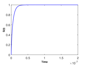
Figure 2: The changes of the entropy of the system versus time.

The probability distribution of diagonal and off-diagonal elements of $\rho_{s}(t)$ in (22) can be obtained as $\text{Pr}(X)=\langle X|\rho_{s}(t)|X\rangle$ and $\text{Pr}(P)=\langle P|\rho_{s}(t)|P\rangle$, respectively. We expect the well-separated two peaks along $X$ axis, representing the pointer positions at the detectors D1 and D2 (See FIG. 3). Therefore, the ratio of the peak heights shows the ratio of times which the detectors click. For the system described by the density matrix (22), the interference fringes along $P$ axis can be depicted by the following relation

$$\text{Pr}(P)=\sqrt{\frac{1}{\Omega\pi}}e^{-\frac{P^{2}}{\Omega}}[1 +\frac{\eta^{2}-1}{2\bar{n}+1}\sin(Pd)$$

$$+\eta\sin\phi\cos(Pd)],$$ (25)

where $d$ represents the differences of the optical path lengths between the detectors.

Two important terms appear in the momentum probability (IV). First the term including ”$\eta\sin\phi\cos(Pd)$” which has the main role in the appearance of the interference pattern. By passing time, $\eta$ tends to zero and as we expect, the interference pattern vanishes after a certain time known as decoherence time, as is shown in FIG. 3. Moreover, choosing the phase factor $\phi=0$, the mentioned term is zero again and no interference appears. However, as we see in FIG. 3, at the beginning time ($t=0$) with $\phi=0$, only one detector clicks an no interference pattern is observed before the decoherence works.

The second term ”$\frac{\eta^{2}-1}{2\bar{n}+1}\sin(Pd)$” is at $t=0$ (with $\eta\approx 1$) negligible compared to the term mentioned above because $\bar{n}$ is in the denominator. This term has also a definite contribution in the appearance of the interference pattern, though it is partial. Yet, when time passes and the decoherence begins to work and/or one chooses the phase factor $\phi$ to be zero, its contribution could be significant, especially in situations where $\bar{n}$ is small.

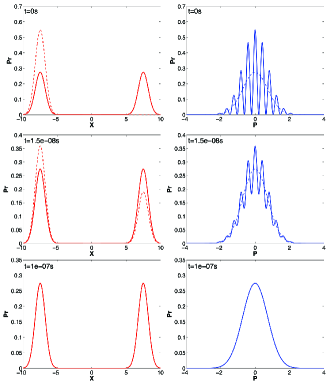
Figure 3: The position (left side) and the momentum (right side) distribution functions of the system at $t=0s$, $1.5\times 10^{-8}s$ and $1\times 10^{-7}s$ with $\Omega/T=10^{10}s^{-1}K^{-1}$. The solid line shows the evolution for the phase factor $\phi=\pi/2$, and the dashed line is for $\phi=0$.

V Results and Discussion

Let us discuss and conclude fundamentally important effects of the thermal bath on the system. If one considers the interference pattern equation (IV) for $\phi=0$ or after the decoherence process when $\eta=0$, in both of these situations the term ”$\frac{\eta^{2}-1}{2\bar{n}+1}\sin(Pd)$” will have a significant role in the appearance of the interference pattern, especially for small values of $\bar{n}$. The condition $\phi=0$ helps us to compare the problem with the case in which we have a closed system with no interference. Also, $\eta=0$ makes us sure that we have the most influence of the thermal bath on the system. With $\phi=0$, we just have the term ”$\frac{\eta^{2}-1}{2\bar{n}+1}\sin(Pd)$”, which is zero at $t=0$, but when time goes on, especially after the decoherence process, it reaches the maximum value of ”$\frac{-1}{2\bar{n}+1}\sin(Pd)$”.

Let us now consider the entropy function in such a situation. After the decoherence process, entropy tends to the following constant value

$$S(t\rightarrow\infty)=-\frac{\bar{n}+1}{2\bar{n}+1}\log_{2}\frac{\bar{n}+1}{2\bar{n}+1}-\frac{\bar{n}}{2\bar{n}+1}\log_{2}\frac{\bar{n}}{2\bar{n}+1}.$$ (26)

For large values of $\bar{n}$ (at high temperatures, or more precisely, low $\Omega/T$), the entropy value approaches $1$. When a system is in a completely mixed state with equal probabilities of its eigenvectors, the entropy has a maximum value, which for the two-dimensional Hilbert state is $1$. FIG. 3 shows us that the decoherence makes this possible that the system has a chance to be found in another state (i.e., $|0\rangle$) too since both detectors have the same chance to click when the decoherence process is completed. Yet, when $\Omega/T$ is large enough, $S(t\rightarrow\infty)$ is far from $1$ and the state of the system is not completely mixed, as is described by the interference pattern equation (IV). Even after the decoherence process is completed, high values of $\Omega/T$ cause the interference pattern appear, due to the term ”$\frac{-1}{2\bar{n}+1}\sin(Pd)$”. This is interesting because we have the classical perception of a thermalized state. During decoherence the state goes into a thermalization process and ended in a mixed thermalized state which called classical because it loses its quantum properties and has no coherency itself. Thus, we have no expectation to see any coherency in the system. However, it seems that the state of the system measuring in different basis may cause it shows some coherency that is in contrast with the classical interpretation of the thermalized state Jeo ; Jeo2 . This indeed changes our attitude about the meaning of decoherence as the quantum-to-classical transition. Somehow, this shows that the system affected by the environment keeps some of its quantum properties. So, it seems that actually, the maximization of the entropy happens during the decoherence process.

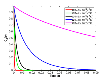
Figure 4: The distillable coherence $C_{d}(\rho)$ versus time with different values of $\Omega/T$. As time goes on, the larger $\Omega/T$ causes the distillable coherence decreases with a lower slope.

For investigating the system coherency in this setup, one can use the distillable coherence $C_{d}(\varrho)$ as a quantifier Win . The distillable coherence is the optimum number of maximally coherent states which can be obtained from a state $\varrho$ using incoherent operations. It has been shown that the distillable coherence can simply write as Win ; Str

$$C_{d}(\varrho)=S(\Xi[\varrho])-S(\varrho),$$ (27)

where $\Xi[\varrho]=\sum_{i=0}^{d-1}|i\rangle\langle i|\varrho|i\rangle\langle i|$ is the dephasing operator. In the case of the density matrix, $\rho$ mentioned in equation (22), for the entropy of the dephased density matrix we have

$$S(\Xi[\rho])=- \sum_{i=0,1}[\frac{1+(-1)^{i}\eta\cos\phi}{2}$$

$$\times\log(\frac{1+(-1)^{i}\eta\cos\phi}{2})].$$ (28)

Therefore, because of (IV), the distillable coherency $C_{d}(\rho)$ can be calculated for the system with different $\Omega/T$. As we expected, the value of the $C_{d}(\rho)$ decreases as time goes on. However, as FIG. 4 shows the large values of $\Omega/T$ cause the system remains coherent for a long time. If one considers $\Omega/T$ to be large enough, the distillable coherence almost remains invariant and the system stays coherent. So, we can observe the interference patterns after the decoherence process, as is represented in FIG. 5. This is interesting that although the decoherence effect disrupts the coherency, this setup makes it possible to bring back the coherency keeping the quantum properties alive. Observing coherency for the system after the decoherence process makes our interpretation of the thermalized state as a classical mixture ambiguous. Here, we showed that by measuring the system on a different basis one can still see coherency in the system. Therefore, the system in a thermalization process does not necessarily end up in a classical state.

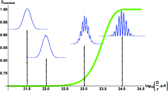
Figure 5: Remained entropy ($S_{rem}$) changes versus $\log(\frac{\Omega}{T}.s.K)$. The interference patterns are illustrated among the remained entropy with $\log(\frac{\Omega}{T}.s.K)=21.5$, $22$, $23$ and $24$. The phase factor $\phi$ is taken zero here.

To examine the classicality of the resulted state we calculate the degree of mixedness ($M=1-\text{Tr}[\rho^{2}]$) of the system exactly after its interaction with thermal bath with the density matrix (21) in the limit of $t\rightarrow\infty$ or $\eta\rightarrow 0$. Fortunately, the degree of the mixedness of the system is near zero at low temperatures which shows that the system is completely coherent, although its density matrix is diagonal. FIG. 6 shows the changes of $M$ versus temperature in which with the increasing of the temperature the system ends up in the mixed state as the degree of mixedness approaches to $M=0.5$. Furthermore, the visibility $v$ of the interference fringes (FIG. 5) is defined as Walls $v=(I_{max}-I_{min})/(I_{max}+I_{min})$ where $I_{max(min)}$ is the maximum (minimum) intensities on the detectors. We sketched $v(\tau)$ along with time in FIG. 6. $\tau$ represents the time interval between the detectors. As we expect, the visibility is $1$ before the decoherence process starts. Interestingly, as FIG. 6 shows, by setting an appropriate time interval we could reach the visibility near $1$ even when the decoherence process completed. It is obvious that the interference fringes with high visibility are incompatible with classical physics and evidence of quantum coherence Jeo .

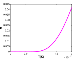
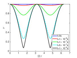
Figure 6: (a) The changes of the degree of mixedness ($M$) versus temperature. The system remains coherent at low temperatures (b) The interference fringes versus the time interval ($\tau$) as the decoherence process evolves with time. We considered $\Omega=1\times 10^{12}$.

Here, we introduce a measure to see how much the system keeps its quantum properties. This helps us to have a better understanding of the emergence of the classical traits. This is based on the distance of system’s maximum entropy with the entropy of the system in a completely mixed state which we call it the remained entropy, $S_{rem}$:

$$S_{rem}:=S_{cm}-S(t\rightarrow\infty),$$ (29)

where $S_{cm}$ is the entropy of a completely mixed state and its value is $1$ in our case. The greater the amount of the remained entropy is the more quantum properties the system shows. In this regard, FIG. 5 shows that with growing the remained entropy, the interference pattern due to the effects of the environment (caused by the term ”$\frac{-1}{2\bar{n}+1}\sin(Pd)$” ) appears more distinctly. Not generally, but in this case which the completely mixes state is a Gaussian distribution, the remained entropy is the negentropy of the system at $t\rightarrow\infty$. The remained entropy shows the distance of the thermalized state from the classical mixture which it does not show any coherency in any basis. However, by getting away from a classical mixture, we hope to see the coherence. As we expect, with higher remained entropy, the distillable coherency decays slower.

The remained entropy shows us that a quantum system after the effect of the environment does not completely lose its quantum properties and always there remains a distance to the complete mixed state, though small. Yet, this does not necessarily mean that a classical situation is attained. What really happens is that the system-bath interaction leads the system to the maximum possible entropy.

References

- (1) M. Goldstein and F. I. Goldstein, The Refrigerator and the Universe, Harvard University Press, Cambridge (1993).
- (2) N. Liu, J. Goold, I. Fuentes, V. Vedral, K. Modi, D.E. Bruschi, Class. Quantum Grav. 33, 035003 (2016).
- (3) J. Gemmer, M. Michel and G. Mahler, Quantum Thermodynamics: Emergence of Thermodynamic Behavior Within Composite Quantum Systems, Lect. Notes Phys. 784, Springer, Berlin Heidelberg (2009).
- (4) J. Goold, M. Huber, A. Riera, L. del Rio and P. Skrzypczyk, J. Phys. A: Math. and Theo. 49, 143001 (2016).
- (5) S. Vinjanampathy and J. Anders, Cont. Phys. 57, 545-579 (2016).
- (6) S. Trotzky, Y. A. Chen, A. Flesch, I. P. McCulloch, U. Schollwöck, J. Eisert and I. Bloch, Nat. Phys. 8, 325-330 (2012).
- (7) U. Schollwöck, Ann. Phys. 326, 96-192 (2011).
- (8) C. Jarzynski, Phys. Rev. Lett. 78, 2690 (1997).
- (9) G. E. Crooks, Phys. Rev. E 60, 2721 (1999).
- (10) S. Popescu, A. J. Short and A. Winter, Nat. Phys. 2, 754-758 (2006).
- (11) L. del Rio, J. Aberg, R. Renner, O. Dahlsten and V. Vedral, Nature 474, 61-63 (2011).
- (12) F. G. Brandao, M. Horodecki, J. Oppenheim, J. M. Renes and R. W. Spekkens, Phys. Rev. Lett. 111, 250404 (2013).
- (13) T. M. Nieuwenhuizen and A. E. Allahverdyan, Phys. Rev. E 66, 036102 (2002).
- (14) J. Anders and V. Giovannetti, New J. Phys. 15, 033022 (2013).
- (15) A. E. Allahverdyan and T. M. Nieuwenhuizen, Phys. Rev. E 71, 066102 (2005).
- (16) M. Esposito and S.Mukamel, Phys. Rev. E 73 046129 (2006).
- (17) P. Talkner, E. Lutz and P. Hanggi, Phys. Rev. E 75, 050102 (2007).
- (18) W. Pusz and S. Woronowicz, Comm. Math. Phys. 58, 273-290 (1978).
- (19) M. J. Henrich, G. Mahler and M. Michel, Phys. Rev. E 75, 051118 (2007).
- (20) H. Weimer, M. J. Henrich, F. Rempp, H. Schröder and G. Mahler, Europhys. Lett. 83, 30008 (2008).
- (21) J. Deutsch, New J. Phys. 12, 075021 (2010).
- (22) M. Esposito, K. Lindenberg and C. Van den Broeck, New J. Phys. 12, 013013 (2010).
- (23) M. Esposito and C. Van den Broeck, Europhys. Lett. 95, 40004 (2011).
- (24) J. Gemmer and R. Steinigeweg, Phys. Rev. E 89, 042113 (2014).
- (25) H. Wilming, R. Gallego and J. Eisert, Phys. Rev. E 93, 042126 (2016).
- (26) J. P. Santos, G. T. Landi and M. Paternostro, Phys. Rev. Lett. 118, 220601 (2017).
- (27) A. E. Allahverdyan and T. M. Nieuwenhuizen, Phys. Rev. Lett. 85, 1799 (2000).
- (28) S. Hilt and E. Lutz, Phys. Rev. A 79, 010101 (2009).
- (29) P. Faist, J. Oppenheim and R. Renner, New J. Phys. 17, 043003 (2015).
- (30) C. Hörhammer and H. Büttner, J. Stat. Phys. 133, 1161-1174 (2008).
- (31) J. Goold, M. Huber, A. Riera, L. del Rio, P. Skrzypczyk, J. Phys. A: Math. Theor. 49, 143001 (2016).
- (32) T. M. Cover and J. A. Thomas, Elements of information theory, John Wiley and sons (2006).
- (33) T. Fritz, arXiv:1504.03661 (2015).
- (34) N. Linden, S. Popescu, A. J. Short, and A. Winter, Phys. Rev. E 79, 061103 (2009).
- (35) A. J. Short and T. C. Farrelly, New J. Phys. 14, 013063 (2012).
- (36) A. Riera, C. Gogolin, and J. Eisert, Phys. Rev. Lett. 108, 08040 (2012).
- (37) M. Horodecki and J. Oppenheim, Int. J.Mod. Phys. 27, 1345019 (2012).
- (38) F. Binder, S. Vinjanampathy, K. Modi and J. Goold, Phys. Rev. E 91, 032119 (2015).
- (39) S. Maniscalco, J. Piilo, F. Intravaia, F. Petruccione and A. Messina, Phys. Rev. A 70, 032113 (2004).
- (40) V. Gorini, A. Kossakowski, and E.C.G. Sudarshan, J. Math. Phys. 17, 821 (1976).
- (41) H. P. Breuer and F. Petruccione, The Theory of Open Quantum Systems Oxford University Press (2002).
- (42) S. Maniscalco, F. Intravia, J. Piilo, and A. Messina, J. Opt. B: Quantum Semiclassical Opt. 6, S98 (2004).
- (43) M. A. Schlosshauer, Decoherence: and the Quantum-to-Classical Transition, Springer Science & Business Media (2007).
- (44) T. Hatano and S. I. Sasa, Phys. Rev. Lett. 86, 3463 (2001).
- (45) T. Sagawa, Lect. Quantum Comput. Thermodyn. Stat. Phys. 8, 125 (2012).
- (46) V. Vedral, Rev. Mod. Phys. 74, 197 (2002).
- (47) G.Lindblad, Commun. Math. Phys. 40, 147, (1975).
- (48) H. Jeong and T. C. Ralph, Phys. Rev. Lett. 97, 100401 (2006).
- (49) H. Jeong and T. C. Ralph, Phys. Rev. A 76, 042103 (2007).
- (50) A. Winter and D. Yang, Phys. Rev. Lett. 116, 120404 (2016).
- (51) A. Streltsov, G. Adesso and M.B. Plenio, Rev. Mod. Phys. 89, 041003 (2017).
- (52) D. F. Walls and G. J. Milburn, Quantum Optics, Springer-Verlag (1994).