Abstract

In this contribution, we introduce a technique to freeze the parameters which describe the accelerated states between two users to be used in the context of quantum cryptography and quantum teleportation. It is assumed that, the two users share different dimension sizes of particles, where we consider a qubit-qutrit system. This technique depends on local operations, where it is allowed that each particle interacts locally with a noisy phase channel. We show that, the possibility of freezing the information of quantum channel between the users depends on the initial state setting parameters, the initial acceleration parameter strength of the phase channel. It is shown that, one may increase the possibility of freezing the estimation degree of the parameters if only the larger dimension system or both particles pass through the noisy phase channel. Moreover, at small values of initial acceleration and large values of the channel strength, the size of freezing estimation areas increases. The results may be helpful in the context of quantum teleportation and quantum coding.

1 INTRODUCTION

It is well known that, to perform some quantum information tasks as teleportation[1], cryptography [2], quantum encoding [3, 4] and computations [5] , one needs to generate maximum entangled states. Practically, it is possible to generate these states, but during their transmission from the source to the users they interact with their surrounds and consequently the coherence takes place. Therefore, these maximum entangled states turn into partially entangled states and consequently, their efficiency to perform the quantum information tasks decrease. There are different types of noise which cause this decoherence. One of the noisy channel is the Unruh effect which is represented by the acceleration [6]. There are several studies that have been done to investigate the behavior of the accelerated systems in different types of noise. The possibility of using these accelerated systems to implement quantum teleportation is discussed by Metwally [7]. Using the accelerated system to perform quantum encoding is investigated in[8]. However, some protocols were introduced to minimize the losses of the coherence of the accelerated systems. Metwally [9] suggested a protocol based on weak and reverse measurement to enhance the local and non-local information of accelerated two different dimension systems. Bromely et. al [10] discussed the possibility of freezing the quantum coherence of two qubit systems in the presence of different noisy channels. Recently M.-Ming Du et. al [11] investigated the Unruh effect on the coherence dynamics of accelerated qubit systems.

As the information of any system is contained in its parameters, we can minimize the possibility of estimating these parameters or freezing the degree of estimation during the transmission process from one location to another. In this case, if the travelling states are captured by adversary, then may he/she get a minimum information or nothing at all. Moreover, the adversary cannot dissipate the information and consequently cannot strayed the users be sending different information.

Here, we introduce a technique to freeze the decoherence due to the acceleration. In this context, a system consists of qubit-qutrit, where it is assumed that only the qubit is accelerated with a uniform acceleration while the qutrit state in the inertial frame. In this protocol, we freeze the information which can be find on the parameters which describe the accelerated state. The main idea of this technique is to allow one or each of these particles (qubit/qutrit) to pass through a noisy phase channel. We estimate the initial values of the initial parameter settings and the strength of the noisy channel that maximize, minimize and freezing the accelerated state.

The paper is organized as follows. In Sec.II, we describe the quantum state that is shared between the two users; (Alice) and (Bob). In Sec. III,the acceleration process is briefly described. The paper is organized as follows. In Sec.II, we describe the quantum state that is shared between the users; Alice and Bob. In Sec. III, the acceleration process is described briefly. The possibility of estimating the initial parameters by using quantum Fisher information. Finally we discuss our results in Sec. IV.

2 The suggested quantum system

2.1 qubit-qutrit system

We assume that the system consists of a qubit(two-levels) system and a qubit (three-levels system) are initially prepared in an entangled state. In the computational basis $\{0,~{}1\}$, for the single qubit and $0,1,2$ for the single qutrit, one can write the density operator of qubit-qutrit system in the basis$\bigl{|}00\bigr{\rangle},\bigl{|}01\bigr{\rangle},\bigl{|}02\bigr{\rangle},\bigl{|}10\bigr{\rangle},\bigl{|}11\bigr{\rangle}$ and $\bigl{|}12\bigr{\rangle}$ as

$$\rho_{ab} = \Bigl{\{}\frac{\mu}{2}(\bigl{|}0\bigr{\rangle}_{a}\bigl{\langle}0\bigr{|}+\bigl{|}1\bigr{\rangle}_{a}\bigl{\langle}1\bigr{|})\Bigl{\}}\otimes\bigl{|}1\bigr{\rangle}_{b}\bigl{\langle}1\bigr{|}+\Bigl{\{}\frac{\mu}{2}\bigl{|}1\bigr{\rangle}_{a}\bigl{\langle}1\bigr{|}+\frac{1-2\mu}{2}\bigl{|}0\bigr{\rangle}_{a}\bigl{\langle}0\bigr{|}\Bigr{\}}\otimes\bigl{|}2\bigr{\rangle}_{b}\bigl{\langle}2\bigr{|}$$ (1)

$$+ \Bigl{\{}\frac{\mu}{2}\bigl{|}0\bigr{\rangle}_{a}\bigl{\langle}1\bigr{|}+\frac{1-2\mu}{2}\bigl{|}1\bigr{\rangle}_{a}\bigl{\langle}0\bigr{|}\Bigr{\}}\otimes\bigl{|}0\bigr{\rangle}_{b}\bigl{\langle}2\bigr{|}+\Bigl{\{}\frac{\mu}{2}\bigl{|}1\bigr{\rangle}_{a}\bigl{\langle}0\bigr{|}+\frac{1-2\mu}{2}\bigl{|}0\bigr{\rangle}_{a}\bigl{\langle}1\bigr{|}\Bigr{\}}\otimes\bigl{|}2\bigr{\rangle}_{b}\bigl{\langle}0\bigr{|}$$

$$+ \Bigl{\{}\frac{\mu}{2}\bigl{|}0\bigr{\rangle}_{a}\bigl{\langle}0\bigr{|}\Bigr{\}}\otimes\bigl{|}0\bigr{\rangle}_{b}\bigl{\langle}0\bigr{|}+\Bigl{\{}\frac{1-2\mu}{2}\bigl{|}1\bigr{\rangle}_{a}\bigl{\langle}0\bigr{|}\Bigr{\}}\otimes\bigl{|}0\bigr{\rangle}_{b}\bigl{\langle}1\bigr{|},$$

where, $0\leq\mu\leq\frac{1}{2}$ [14]. All the information of this density operator is encoded in the parameter $\mu$, which represents the initial state setting parameter.

2.2 Acceleration process

In this context, we assume that only Alice qubit is accelerated with a uniform acceleration $r$, while Bob’s qutrit stays in the inertial. This means that, Alice qubit will be in Minkowski space, Therefore, if the coordinate of a particle is defined by $(t,z)$ in Minkowski space, then in Rindler space, the Dirac qubits coordinates may be defined by $(\tau,x)$, where

$$\tau=a\tanh(t/z),\quad x=\sqrt{z^{2}-t^{2}},$$ (2)

and $\quad-\infty<r<\infty,\quad-\infty<x<\infty$, $\tan r_{b}=exp[-\pi\omega\frac{c}{a_{c}}]$,  $0\leq r\leq\pi/4$, $-\infty\leq a_{c}\leq\infty$, $\omega$ is the frequency, $c$ is the speed of light [12]. The computational basis $\bigl{|}0_{k}\bigr{\rangle}$and $\bigl{|}1_{k}\bigr{\rangle}$ can be written as [15, 13, 14],

$$\bigl{|}0_{M}\bigr{\rangle} = \cos r\bigl{|}0_{R}\bigr{\rangle}_{I}\bigl{|}0_{R}\bigr{\rangle}_{II}+\sin r\bigl{|}1_{R}\bigr{\rangle}_{I}\bigl{|}1_{R}\bigr{\rangle}_{II},$$

$$\bigl{|}1_{M}\bigr{\rangle} = \bigl{|}1_{R}\bigr{\rangle}_{I}\bigl{|}0_{R}\bigr{\rangle}_{II}.$$ (3)

Now, using the transformation (2.2) and the initial state (1), the final accelerated state is given by

$$\rho_{ab}^{ac} = \varrho_{1}\bigl{|}00\bigr{\rangle}\bigl{\langle}00\bigr{|}+\varrho_{2}\bigl{|}01\bigr{\rangle}\bigl{\langle}01\bigr{|}+\varrho_{3}\bigl{|}00\bigr{\rangle}\bigl{\langle}12\bigr{|}+\varrho_{4}\bigl{|}12\bigr{\rangle}\bigl{\langle}00\bigr{|}+\varrho_{5}\bigl{|}10\bigr{\rangle}\bigl{\langle}02\bigr{|}+\varrho_{6}\bigl{|}02\bigr{\rangle}\bigl{\langle}10\bigr{|}$$ (4)

$$+\varrho_{7}\bigl{|}02\bigr{\rangle}\bigl{\langle}02\bigr{|}+\varrho_{8}\bigl{|}10\bigr{\rangle}\bigl{\langle}10\bigr{|}+\varrho_{9}\bigl{|}12\bigr{\rangle}\bigl{\langle}12\bigr{|}+\varrho_{10}\bigl{|}11\bigr{\rangle}\bigl{\langle}11\bigr{|}$$

where,

$$\varrho_{1} = \varrho_{2}=\frac{\mu}{2}\cos^{2}r,\quad\varrho_{3}=\varrho_{4}=\frac{\mu}{2}\cos r,\quad\varrho_{5}=\varrho_{6}=\frac{1-2\mu}{2}\cos r,\quad$$

$$\varrho_{7} = \frac{1-2\mu}{2}\cos^{2}r,~{}\varrho_{8}=\frac{1-2\mu}{2}+\frac{\mu}{2}\sin^{2}r,\quad$$

$$\varrho_{9} = \frac{\mu}{2}+\frac{1-2\mu}{2}\sin^{2}r,\varrho_{10}=\frac{\mu}{2}(1+\sin^{2}r).$$ (5)

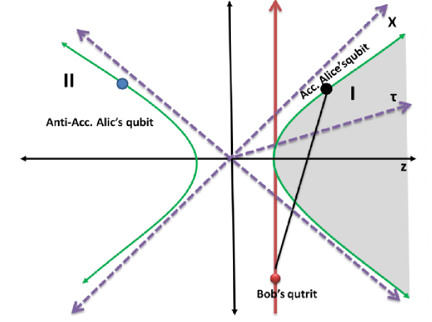
Figure 1: This diagram shows the dynamics of the accelerated particle in the Rindler space-time. The accelerated particle travels on a hyperbola in the first region, $I$ with a uniform acceleration, while its anti-particle travels in the second region, $II$. The non-accelerated particle stays in the inertial frame.

2.3 Phase channel

For a single qubit, the phase-flip channel in the computational basis set $\{0,~{}1,~{}2\}$ may be described by [21],

$$\mathcal{K}_{1}^{a}=\mathcal{P}_{1}I_{2\times 2}\otimes I_{3\times 3},\quad\mathcal{K}_{2}^{a}=\mathcal{P}_{2}\sigma_{z}\otimes I_{3\otimes 3}$$ (6)

where $\mathcal{P}_{1}^{2}+\mathcal{P}_{2}^{2}=1$ and $I_{2\otimes 2},I_{3\otimes 3}$ are the units operators of the qubit and the qutrit, respectively, y $\mathcal{P}_{1}=\sqrt{1-\frac{\gamma_{a}}{2}}$ and $\gamma_{a}$ is the strength of the phase channel. For the single qutrit system the phase-flip channel is given in the Kraus representation as

$$\mathcal{K}_{1}^{b} = \mathcal{R}_{1}I_{2\times 2}\otimes I_{3\times 3}$$

$$\mathcal{K}_{2}^{b} = \mathcal{R}_{2}I_{2\times 2}\otimes\Bigl{(}\bigl{|}0\bigr{\rangle}\bigl{\langle}0\bigr{|}+e^{-2i\pi/3}\bigl{|}1\bigr{\rangle}\bigl{\langle}1\bigr{|}+e^{2i\pi/3}\bigl{|}2\bigr{\rangle}\bigl{\langle}2\bigr{|}\Bigr{)},\quad$$

$$\mathcal{K}_{3}^{b} = \left(\mathcal{K}_{2}^{b}\right)^{\dagger}$$ (7)

where $\mathcal{R}_{1}=\sqrt{1-\frac{2\gamma_{b}}{3}}$, $\mathcal{R}_{2}=1-\mathcal{R}_{1}^{2}$, and $\gamma_{b}$ is the strength of the channel with respect to the qutrit. Now, we have different possibility, either the qubit or the qutrit passes through the phase channel or both of them are forced to pass through these noisy channels.

Now, let assume that the accelerated qubit-qutrit system (4) passes through the phase-flip channel. The output state is given by

$$\rho_{F} = \sum_{J=1}^{3}\sum_{i=1}^{2}\left\{\mathcal{R}^{b}_{j}\mathcal{K}^{a}_{i}\rho_{ab}\Bigl{(}{\mathcal{K}_{i}^{a}}\Bigr{)}^{\dagger}\Bigl{(}{\mathcal{R}_{j}^{b}}\Bigr{)}^{\dagger}\right\}$$ (8)

In the computational basis the final state (8) is given by

$$\rho_{F} = \varrho_{1}\bigl{|}00\bigr{\rangle}\bigl{\langle}00\bigr{|}+\varrho_{2}\bigl{|}01\bigr{\rangle}\bigl{\langle}01\bigr{|}+\varrho_{7}\bigl{|}02\bigr{\rangle}\bigl{\langle}02\bigr{|}+\varrho_{8}\bigl{|}10\bigr{\rangle}\bigl{\langle}10\bigr{|}+\varrho_{10}\bigl{|}11\bigr{\rangle}\bigl{\langle}11\bigr{|}$$ (9)

$$+ \varrho_{9}\bigl{|}12\bigr{\rangle}\bigl{\langle}12\bigr{|}+(1-\gamma_{a})\eta_{b}\Bigl{(}\varrho_{3}\bigl{|}00\bigr{\rangle}\bigl{\langle}12\bigr{|}+\varrho_{4}\bigl{|}12\bigr{\rangle}\bigl{|}00\bigr{\rangle}+\varrho_{5}\bigl{|}10\bigr{\rangle}\bigl{\langle}02\bigr{|}+\varrho_{6}\bigl{|}02\bigr{\rangle}\bigl{\langle}10\bigr{|}\Bigr{)}$$

where $\eta_{b}=1-\frac{2\gamma_{b}}{3}(1-\cos(2\pi/3))$.

The main task now is estimating the initial parameter of the state settings, $(\mu)$ and of the initial strength channels, $\gamma$ , where we set $\gamma_{a}=\gamma_{b}=\gamma$.

3 Fisher Information

3.1 Mathematical Form

Quantum Fisher information represents a central role in the estimation theory, where it can be used to quantify some parameters that cannot be quantified directly [16]. In this subsection, we review the mathematical form of Fisher information. Let $\eta$ be the parameter to be estimated. The spectral decomposition of the density operator is given by $\rho_{\eta}=\sum_{j=1}^{n}\kappa_{j}\bigl{|}\psi_{j}\bigr{\rangle}\bigl{\langle}\psi_{j}\bigr{|}$, where $\kappa_{j}$and $\bigl{|}\psi_{j}\bigr{\rangle}$ are the eigenvalues and the corresponding eigenvectors of the state $\rho_{\eta}$. The Fisher information with respect to the parameter $\eta$ is defined as [20]

$$\mathcal{F}_{\eta}=tr\{\rho_{\eta}L^{2}_{\eta}\},~{}$$ (10)

where the symmetric logarithmic derivative $L_{\eta}$ is a solution to the equation $\frac{\partial\rho_{\eta}}{\partial\eta}=\frac{1}{2}(\rho_{\eta}L_{\eta}+L_{\kappa}\rho_{\kappa})$. Using the spectral decomposition and the identity $\sum_{j=1}^{n}\bigl{|}\psi_{j}\bigr{\rangle}\bigl{\langle}\psi_{j}\bigr{|}=1$ in Eq.(5), one can obtain the final form of the Fisher information as[17, 18, 19],

$$\mathcal{F}=\mathcal{F}_{cl}+\mathcal{F}_{qu}-\mathcal{F}_{mix},$$ (11)

where

$$\mathcal{F}_{cl} = \sum_{j=1}^{n}\frac{1}{\kappa_{j}}\left(\frac{\partial\kappa_{j}}{\partial\eta}\right)^{2},$$

$$\mathcal{F}_{qu} = 4\sum_{j=1}^{n}\kappa_{j}\Bigl{(}\left\langle\frac{\partial\psi_{j}}{\partial\eta}\Big{|}\frac{\partial\psi_{j}}{\partial\eta}\right\rangle-\Bigl{|}\left\langle\psi_{j}\Big{|}\frac{\partial\psi_{j}}{\partial\eta}\right\rangle\Bigr{|}^{2}\Bigr{)},$$

$$\mathcal{F}_{mix} = 8\sum_{j\neq\ell}^{n}\frac{\kappa_{j}\kappa_{\ell}}{\kappa_{j}+\kappa_{\ell}}\Big{|}\left\langle\psi_{j}|\frac{\partial\psi_{\ell}}{\partial\eta}\right\rangle\Big{|}^{2}.$$ (12)

The summations on the first and the third terms over all $\kappa_{j}\neq 0$ and $\kappa_{j}+\kappa_{\ell}\neq 0$. The first and the second terms represent the classical Fisher information, $(\mathcal{F}_{c})$, and the quantum Fisher information of all pure states, $(\mathcal{F}_{p})$, respectively. The third term, $(\mathcal{F}_{m})$ is stemmed from the mixture of the pure states. It is clear that, Fisher information for a pure state is just the first two terms, namely $\mathcal{F}_{pure}=\mathcal{F}_{c}+\mathcal{F}_{p}$, while for a mixed state the third term is subtracted. Therefore, the quantum Fisher of a pure state is larger than that displayed for a mixed state [17, 18, 19].

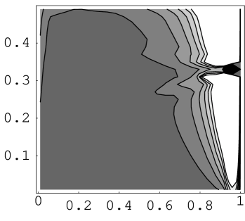
Figure 2: Fisher information with respect to the acceleration parameter, $\mathcal{F}_{r}$ where the initial acceleration (a) $r=0.1$ and (b)$r=0.2$.

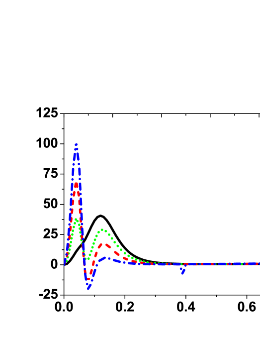
Figure 3: Fisher information, $\mathcal{F}_{r}$ for an accelerated system initially prepared $\gamma=0.99$ and $\mu=0.01,0.1,0.2,3$ for the solid, dot, dash and dash-dot, respectively.

3.2 Only the qubit passes through the phase channel

Fig.(2a) displays the behavior of the quantum Fisher information $\mathcal{F}_{r}$ for any initial state settings and initial channel strength $\gamma$ at a small initial value of the acceleration $(r=0.1)$. The degree of the darkness displays the possibility of estimating the parameter $r$. However, as the brightness increases the estimation’s degree of the parameter $r$ increases. Different regions show that, the Fisher information $\mathcal{F}_{r}$ is frozen. Fig.(2b) displays the behavior of $\mathcal{F}_{r}$ at larger values of the initial acceleration where we set $r=0.2$. In general, the behavior is similar to that displayed in Fig.(2a). However, the size of the estimation areas are changed and irregularity takes place.

From Fig.(2), for small values of the initial acceleration, the sizes of the frozen areas are wider than those displayed at larger values of initial acceleration.

In Fig.(3), we show the effect of maximum value of channel strength on $\mathcal{F}_{r}$, where we set $\gamma_{a}=0.99$. At zero acceleration, the Fisher information increases suddenly for any initial state setting to reach its maximum values. These maximum values depend on the initial state settings, where they are higher at larger values of $\mu$. However, at smaller values of $r$, the sudden decay phenomena is predicted at larger values of $\mu$. Moreover, the behavior of the quantum Fisher information, $\mathcal{F}_{r}$ is almost frozen as one increases the acceleration.

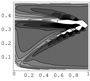
Figure 4: (a)The Fisher information with respect to the initial state setting parameter $\mu$ at an initial acceleration $r=0.2$. (b)Fisher information $\mathcal{F}\mu$, where $\gamma=0.99$ and $\mu=0.05,0.1,0.15,0.2$ for the dot, dash, dash-dot and solid, respectively

Fig(4a) shows the values of $\mu$ and$\gamma$ that freeze the quantum Fisher information with respect to the initial state setting parameter $\mu$. Different degrees of darkness are displayed. This means that, in these regions the quantum Fisher information is frozen. The degree of brightness increases at larger values of $\mu$ and $\gamma$. Fig.(4b) shows the frozen effect of the channel and the gradual increasing of $\mathcal{F}_{\mu}$ as the acceleration increases. However, the increasing rate of $\mathcal{F}_{\mu}$ increases for smaller values of the initial state parameter $\mu$ and larger values of $r$.

3.3 Only the Qutrit passes through the phase channel

. Figs.(5) display the areas in which one may estimate the acceleration parameter by means of the quantum Fisher information $\mathcal{F}_{r}$. It is clear that, the degree of brightness increases as $\mu$ and $r$ increase. The similar color degree means that in these regions the Fisher information is Frozen . The size of the regions depend on the initial acceleration, e.g. at $r=0.5$ the size areas are smaller than that displayed at $r=0.1$. Also, at large values of $\mu$ or $r$, the possibility of estimating the acceleration parameter $r$ increases.

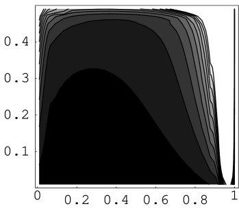
Figure 5: The Fisher information with respect to the acceleration parameter when only the qutrit passes through the phase channel with(a) $r=0.1$. and (b) $r=0.5$

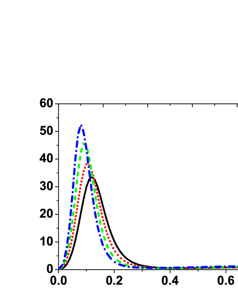
Figure 6: $\mathcal{F}_{r}$ at $\gamma=0.99$ and for different values of $\mu=0.1,0.2,0.3,0.4$ for the solid, dot, dash and dash-dot curves, respectively.

Fig.(6), shows the effect of the maximum value of the channel strength, where we set $\gamma=0.99$. From this figure one sees that, the possibility of estimating the acceleration parameter, $r$, increases as the initial acceleration increases to reach its maximum value. As $r$ increases, the Fisher information $\mathcal{F}_{r}$ decreases gradually and consequently the estimation degree of $r$ decreases as the initial state parameter setting $\mu$ increases. However, the sudden increasing/decreasing behaviors of $\mathcal{F}_{r}$ are displayed for large values of the noise channel strength. The freezing effect of the channel strength is depicted for value of $r\in[0.4,0.8]$ and any initial state parameter settings $\mu$.

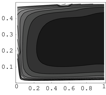
Figure 7: The Fisher information with respect to the initial state settings $\mathcal{F}\mu$ when only the qutrit passes through the phase channel with (a)$r=0.5$ and (b) $r=0.8$.

Fig.(7) displays the effect of different values of the initial acceleration on the estimation degree of the parameter $\mu$. It is clear that, the possibility of estimating $\mu$ increases at small values of $\gamma$ and larger values of $\mu$ or small values of $\mu$ and an arbitrary values of the channel’ strength $\gamma$. The dark areas decrease as $r$ increases, namely, the possibility of freezing the information decreases as $r$ increases.

3.4 The qubit and the Qutrit pass through the phase channel

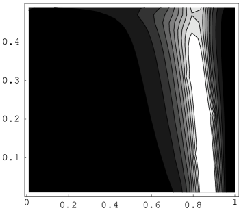
Figure 8: The Fisher information with respect to the acceleration parameter, $\mathcal{F}_{r}$ when both particles pass through the phase channel with (a) $r=0.2$ and (b) $r=0.5$.

It is well know that, the Unruh effect causes a coherence of the accelerated information. Therefor, we investigate the effect of the initial state settings and the channel’ strength at different values of the acceleration. Fig.(8) describes the behavior of the Fisher information with respect to the acceleration parameters. In Fig.(8a), It is assumed that, the qubit is accelerated with a small acceleration, where we set $r=0.1$. It is clear that, for $\mu\leq 6$, and any initial value of channel’ strength, the Fisher information $\mathcal{F}_{\mu}$ is almost frozen. At larger values of $\mu>0.6$, the quantum Fisher information increases gradually to reach its maximum values at $\mu\simeq 0.9$. However, at further values of the channel strength $\gamma$, $\mathcal{F}_{r}$ decreases suddenly to vanish completely at $\mu\simeq 1$ and the frozen behavior is observed again at $\mu=1$.

Fig.(8b), shows the behavior of $\mathcal{F}_{r}$ at larger values of the initial acceleration parameter. It is clear that as $r$ increases, the range of the channel’ strength in which one can freeze the accelerated information decreases. The upper bounds of the quantum Fisher information $\mathcal{F}_{r}$ decreases as the initial acceleration increases. The phenomena of the sudden increase/decrease is displayed for small values of $r$, while the gradual behavior of $\mathcal{F}_{r}$ is depicted for larger values of $r$.

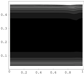
Figure 9: The Fisher information $\mathcal{F}_{\mu}$ when both particle passe through the phase channel with (a) $r=0.1$ and (b) $r=0.5$.

In Fig.(9a), the behavior of the quantum Fisher information $\mathcal{F}_{\mu}$ is displayed for small value of the initial acceleration, where we set $r=0.1$ and arbitrary values of $\mu$ and $\gamma$. It is clear that, at small values of $\gamma$ and $\mu$ the Fisher information $\mathcal{F}_{\mu}$ is maximum. However, as one increases these initial parameters, $\mathcal{F}_{\mu}$ decreases gradually to vanishes completely for $\mu\simeq\in[1.4,3.75]$ and any arbitrary values of the channel’ strength $\gamma$. On the other hand, the sudden increasing behavior of $\mathcal{F}_{\mu}$ is depicted at larger values of the initial state settings, namely $\mu>0.4$ and larger values of the initial channel’ strength ($\gamma>0.8)$.

The bright regions indicate that this parameter may be estimated, while it can’t be estimated in the dark regions. Also, the degree of estimation is almost the same for each region, namely the accelerated channel is frozen. Further, in the dark region the accelerated state is not only frozen but also the estimation degree of $\mu$ is almost zero.

In Fig.(9b), we show that behavior of $\mathcal{F}\mu$ at larger values of the initial acceleration, where we set $r=0.5$. One can estimate the initial state setting parameter $\mu$ in the bright regions and the degree of estimation decreases as the darkness of the region increases. One can also pick the values of the initial parameters which freeze the coherence due to the acceleration $r$.

4 CONCLUSIONS

In this contribution, we estimate the initial state settings and the acceleration that freeze the accelerated state. It is shown that, the degree of estimation depends on either one or both particles are affected by the phase noise channel. If only the qubit is allowed to pass through the phase channel, then one may freeze the information contained in the accelerated state for smaller values of the acceleration, arbitrary initial state settings and arbitrary values of the channel strength. However, at larger values of the acceleration, one may be able to freeze the accelerated state by increasing the channel’ strength. Moreover, the Fisher information with respect to the initial state setting parameter may be frozen at smaller values of initial state settings and larger values of the phase channel strength.

On the other hand, if only the qutrit passes through the phase channel, the areas in which the Fisher information is frozen are more regular and the estimation degree is smaller, where the degree of darkness are much larger than that displayed when only the qubit passes through the phase channel. The frozen areas decrease as the initial acceleration increases. One may also freeze the Fisher information if the phase channel’ strength is large.

Finally, if both particles pass through the phase channel, then at small value of the initial acceleration, the freezing areas are much wider than those displayed in the previous two cases. However, for larger initial acceleration, the possibility of freezing the accelerated Fisher information decreases, where the size of the dark areas decreases. The decreasing rate of theses areas is larger if one estimate the Fisher information with respect to the acceleration parameters. However, the size of the freezing area with respect to the initial state setting parameter is large.

In conclusion, it is possible to minimize or freeze the estimation degree of the parameters which describe the accelerated qubit-qutrit system by using quantum Fisher information. Therefore the travelling state is protect from any Eavesdropper and consequently these state may be useful in context of quantum teleportation and encoding.

References

- [1] C.H. Bennett, G. Brassard, S. Popescu, B. Schumacher, J.A. Smolin, W.K. Wootters,”Purification of Noisy Entanglement and Faithful Teleportation via Noisy Channels”, Phys. Rev. Lett. 76 722 (1996).
- [2] D. Deutsch, A. Ekert, R. Jozsa, C. Macchiavello, S. Popescu, A. Sanpera,”Quantum Privacy Amplification and the Security of Quantum Cryptography over Noisy Channels”, Phys. Rev. Lett. 77 2818 (1996).
- [3] C. H. Bennett and S. J. Wiesner, Phys. Rev. Lett. 69 2881 (1992).
- [4] S. Bose, M. Plenio and V. Vedral, J. Mod. Opt. 47 291 (2000)
- [5] M. A. Nielsen and I. L. Cuand ” Quantum computation and Quantum Information (Cambridge, Cambridge University Press, Cambridge 2000).
- [6] P. M. Alsing, I. F. Schuller, R. B. Mann and T. E. Tessier, ”Entanglement of Dirac fields in noninertial frames,” Phys. Rev. A 74 pp. 032326–032340 (2006).
- [7] N. Metwally, ”Teleportation of accelerated information” J. O. Optic Soc. B (2103).
- [8] N. Metwally and A. Saguher”, Quantum. Inf. Process, 13, 771-780 (2014).
- [9] N. Metwally ” Enhancing entanglement, local and non-local information of accelerated two-qubit and two qutrit” EPL, 116 (2016) 60006.
- [10] T. R. Bromely, M. Cianciarauso, and G. Adesso,” Frozen Quantum Coherence” Phys. Rev. Lett. 114 210401 (2015).
- [11] M.-Ming Du , D. Wang and Liu Ye,” How Unruh effect affects freezing coherence in decoherence” Quantum Inf. Process 16 228 (2017).
- [12] J. Doukas, E. G. Brown, A. J. Dragan, and R. B. Mann, ”Entanglement and discord: Accelerated observations of local and global modes”, Phys. Rev. A 87, 012306 (2013).
- [13] E. M.-Martinez, I. Fuentes,”Redistribution of particle and antiparticle entanglement in noninertial frames”, Phys. Rev. A 83, 052306 (2011).
- [14] N. Metwally,” Entanglement of simultaneous and non-simultaneous accelerated qubit-qutrit systems”, Quantum Inf. and Comput (QIC), 16 0530-0542 (2016).
- [15] N. Friis, A. R. Lee, and D.E. Bruschi,” Fermionic mode entanglement in quantum information”, Phys. Rev. A 87, 022338 (2013).
- [16] P. Yue, Li Ge and Q. Zheng,” Invertible condition of quantum Fisher information matrix for a mixed qubit”, Eur. Phys. J. D. 70 8 (2016).
- [17] X. Xiao, Y. Yao, Wo-J. Zhong, Y. Ling Li and Y.-Mao Xie,” Enhancing teleportation of quantum information by partial measurements”, Phys. Rev. A 93 012307 (2016).
- [18] Y. Yao, X. Xiao, Li Ge, X.-g Wang, and C.-pu Sun,” Quantum Fisher information in non-inertial frames”, Phys. Rev. A 89 042336 (2014).
- [19] W.Zhong, Zhe Sun,Jian Ma, X. Wangand F. Nori,” Fisher information under decoherence in Bloch representation”, Phys. Rev. A 87 022337 (2013).
- [20] C. W. Helstrom,”Quantum Detection and Estimation theory” Academic, New York (1976).
- [21] J.-Liang Gu, Hui Li and G. Lu Long,” Decoherence dynamics of quantum correlations in qubit-qutrit systems”, Quantum Inf. Process 12 3412 (2013).