Reduced Dependency Spaces for Existential Parameterised Boolean Equation Systems

Abstract

A parameterised Boolean equation system (PBES) is a set of equations that defines sets satisfying the equations as the least and/or greatest fixed-points. Thus this system is regarded as a declarative program defining predicates, where a program execution returns whether a given ground atomic formula holds or not. The program execution corresponds to the membership problem of PBESs, which is however undecidable in general.

This paper proposes a subclass of PBESs which expresses universal-quantifiers free formulas, and studies a technique to solve the problem on it. We use the fact that the membership problem is reduced to the problem whether a proof graph exists. To check the latter problem, we introduce a so-called dependency space which is a graph containing all of the minimal proof graphs. Dependency spaces are, however, infinite in general. Thus, we propose some conditions for equivalence relations to preserve the result of the membership problem, then we identify two vertices as the same under the relation. In this sense, dependency spaces possibly result in a finite graph. We show some examples having infinite dependency spaces which are reducible to finite graphs by equivalence relations. We provide a procedure to construct finite dependency spaces and show the soundness of the procedure. We also implement the procedure using an SMT solver and experiment on some examples including a downsized McCarthy 91 function.

1 Introduction

A Parameterised Boolean Equation System (PBES) [14, 11, 13] is a set of equations denoting some sets as the least and/or greatest fixed-points. PBESs can be used as a powerful tool for solving a variety of problems such as process equivalences [2], model checking [14, 12], and so on.

We explain PBESs by an example PBES $\mathcal{E}_{1}$, which consists of the following two equations:

$$\begin{array}[t]{rcl}\nu X(n:N)&=&X(n+1)\vee Y(n)\\ \mu Y(n:N)&=&Y(n+1)\end{array}$$

$X(n:N)$ denotes that $n$ is a natural number and a formal parameter of $X$. Each of the predicate variables $X$ and $Y$ represents a set of natural numbers regarding that $X(n)$ is true if and only if $n$ is in $X$. These sets are determined by the equations, where $\mu$ (resp. $\nu$) is a least (resp. greatest) fixed-point operator. In the PBES $\mathcal{E}_{1}$, $Y$ is an empty set since $Y$ is the least set satisfying that $Y(n)\mathrel{\mathrm{iff}}Y(n+1)$ for any $n\geq 0$. Similarly, $X$ is equal to $\mathbb{N}$ since $X$ is the greatest set satisfying that $X(n)\mathrel{\mathrm{iff}}X(n+1)\vee Y(n)$ for any $n\geq 0$. A PBES is regarded as a declarative program defining predicates. In this example, an execution of the program for an input $X(0)$ outputs true.

The membership problem for PBESs is undecidable in general [14]. Undecidability is proved by a reduction of the model checking problem for the modal $\mu$-calculus with data. Some techniques have been proposed to solve the problem for some subclasses of PBESs: one by instantiating a PBES to a Boolean Equation System (BES) [18], one by calculating invariants [17], and one by constructing a proof graph [5]. In the last method, the membership problem is reduced to an existence of a proof graph. If there exists a finite proof graph for a given instance of the problem, it is not difficult to find it mechanically. However, finite proof graphs do not always exist. A technique is proposed in  [16] that possibly produces a finite reduced proof graph, which represents an infinite proof graph. The technique manages the disjunctive PBESs, in which data-quantifiers are not allowed.

In this paper, we propose a more general subclass, named existential PBESs, and extend the notion of dependency spaces. We discuss the relation between extended dependency spaces and the existence of proof graphs. Dependency spaces are, however, infinite graphs in most cases. Thus we reduce a dependency space for the existential class to a finite one in a more sophisticated way based on the existing technique in [16]. We also give a procedure to construct a reduced dependency space and show the soundness of the procedure. We explain its implementation and an experiment on some examples.

2 PBESs and Proof Graphs

We follow [5] and [13] for basic notions related to PBESs and proof graphs.

We assume a set $\mathcal{DS}$ of data sorts. For every data sort $D\in\mathcal{DS}$, we assume a set $\mathcal{V}_{D}$ of data variables and a semantic domain $\mathbb{D}$ corresponding to it. In this paper, we assume $B,N\in\mathcal{DS}$ corresponding to the Boolean domain $\mathbb{B}=\{\mathbbold{t},\mathbbold{f}\}$ and the natural numbers $\mathbb{N}$, respectively. We use $D$ to represent a sort in $\mathcal{DS}$, $\mathbb{D}$ for the semantic domain corresponding to $D$, and $d$ and $e$ as a data variable in $\mathcal{V}_{D}$. We assume appropriate data functions according to operators, and use ${[\![\mathit{exp}]\!]}\delta$ to represent a value obtained by the evaluation of a data expression $\mathit{exp}$ under a data environment $\delta$. A data expression interpreted to a value in $\mathbb{B}$ is called a Boolean expression. We write ${\bf a}$ or $\overrightarrow{a}$ by using boldfaced font or an arrow to represent a sequence $a_{1},\ldots,a_{n}$ of objects. Especially, ${\bf d}{:}{\bf D}$ is an abbreviation of a sequence $d_{1}{:}D_{1},\dots,d_{n}{:}D_{n}$. We write $\mathbb{D}^{*}$ as a product $\mathbb{D}_{1}\times\cdots\times\mathbb{D}_{n}$ of appropriate domains. In this paper, we use usual operators and constants like $\mathrm{true}$, $\mathrm{false}$, $\leq$, $0$, $1$, $+$, $-$, and so on, along with expected data functions.

A Parameterised Boolean Equation System (PBES) $\mathcal{E}$ is a sequence of well-sorted equations:

$$\left(\sigma_{1}X_{1}({\bf d}{:}{\bf D})=\varphi_{1}\right)\mathrel{\cdots}\left(\sigma_{n}X_{n}({\bf d}{:}{\bf D})=\varphi_{n}\right)$$

where $\varphi_{i}$ is a predicate formula defined by the following BNF, and $\sigma_{i}$ is either one of the quantifiers $\mu,\nu$ used to indicate the least and greatest fixed-points, respectively ($1\leq i\leq n$).

$$\begin{array}[t]{rcl}\varphi&::=&b\ |\ \varphi\wedge\varphi\ |\ \varphi\vee\varphi\ |\ \forall d{:}D\ \varphi\ |\ \exists d{:}D\ \varphi\ |\ X({\bf exp})\end{array}$$

Here $X$ is a predicate variable with fixed arity, $b$ is a Boolean expression, $d$ is a data variable in $\mathcal{V}_{D}$, and ${\bf exp}$ is a sequence of data expressions. We say $\mathcal{E}$ is closed if it does neither contain free predicate variables nor free data variables. Note that the negation is allowed only in expressions $b$ or $\mathit{exp}$ as a data function.

Example 1

A PBES $\mathcal{E}_{2}$ is given as follows:

$$\begin{array}[t]{rcl}\nu X_{1}(n:N)&=&(n=0\wedge X_{1}(n+2))\ \vee\ \left(n>0\wedge X_{2}\left(n-1\right)\wedge X_{1}(n+2)\right)\\ \mu X_{2}(n:N)&=&(n\geq 3\wedge X_{2}(n-2))\ \vee\ \left(n\mathrel{=}1\wedge X_{1}\left(n-1\right)\right)\end{array}$$

Since the definition of the semantics is complex, we omit it and we will explain it by an example. The formal definition can be found in [13]. The meaning of a PBES is determined in the bottom-up order. Considering a PBES $\mathcal{E}_{2}$ in Example 1, we first look at the second equation, which defines a set $X_{2}$. The set $X_{2}$ is fixed depending on the free variable $X_{1}$, i.e., the equation should be read as that $X_{2}$ is the least set satisfying the condition “$v\in X_{2}\ \mathrel{\mathrm{iff}}\ (v\geq 3\wedge v-2\in X_{2})\ \vee\ (v=1\wedge v-1\in X_{1})$” for any $v\in\mathbb{N}$. Thus the set $X_{2}$ is fixed as $\{1,3,5,\dots\}$ if $0\in X_{1}$; $\emptyset$ otherwise, i.e., “$X_{2}(v)\mathrel{\mathrm{iff}}\mathrm{odd}(v)\wedge X_{1}(0)$” for any $v\in\mathbbold{N}$. Next, we replace the occurrence of $X_{2}$ in the first equation of $\mathcal{E}_{2}$ with $\mathrm{odd}(v)\wedge X_{1}(0)$, which results in “$\nu X_{1}(n:N)\ =\ (n=0\wedge X_{1}(n+2))\ \vee\ (n>0\wedge\mathrm{odd}(n-1)\wedge X_{1}(0)\wedge X_{1}(n+2))$”, if we simplify it. The set $X_{1}$ is fixed as the greatest set satisfying that $v\in X_{1}\mathrel{\mathrm{iff}}(v=0\wedge v+2\in X_{1})\ \vee\ (v>0\wedge\mathrm{odd}(v-1)\wedge 0\in X_{1}\wedge v+2\in X_{1})$ for any $v\in\mathbb{N}$. All in all, we obtain $X_{1}=\{0,2,4,\dots\}$ and $X_{2}=\{1,3,5,\dots\}$. The solution ${[\![\mathcal{E}]\!]}$ of a closed PBES $\mathcal{E}$ is a function which takes a predicate variable, and returns a function on $\mathbb{D}^{*}\to\mathbb{B}$ that represents the corresponding predicate determined by the PBES. For instance, in the example PBES $\mathcal{E}_{2}$, ${[\![\mathcal{E}_{2}]\!]}(X_{1})$ is the function on $\mathbb{N}\to\mathbb{B}$ that returns $\mathbbold{t}$ if and only if an even number is given, and ${[\![\mathcal{E}_{2}]\!]}(X_{2})$ is the function on $\mathbb{N}\to\mathbb{B}$ that returns $\mathbbold{t}$ if and only if an odd number is given.

The membership problem for PBESs $\mathcal{E}$ is a problem that answers whether $X({\bf v})$ holds (more formally ${[\![\mathcal{E}]\!]}(X)({\bf v})=\mathbbold{t}$) or not for a given predicate variable $X$ and a value ${\bf v}\in\mathbb{D}^{*}$. The membership problem is characterized by proof graphs introduced in [5]. For a PBES $\mathcal{E}\ =\ \left(\sigma_{1}X_{1}\left({\bf d{:}{\bf D}}\right)=\varphi_{1}\right)\mathrel{\cdots}\left(\sigma_{n}X_{n}\left({\bf d{:}{\bf D}}\right)=\varphi_{n}\right),$ the rank of $X_{i}$ ($1\leq i\leq n$) is the number of alternations of $\mu$ and $\nu$ in the sequence $\nu\sigma_{1}\cdots\sigma_{n}$. Note that the rank of $X_{i}$ bound with $\nu$ is even and the rank of $X_{i}$ bound with $\mu$ is odd. For Example 1, $\mathrm{rank}_{\mathcal{E}_{2}}(X_{1})=0$ and $\mathrm{rank}_{\mathcal{E}_{2}}(X_{2})=1$. Bound variables are predicate variables $X_{i}$ that occur in the left-hand sides of equations in $\mathcal{E}$. The set of bound variables is denoted by $\mathrm{bnd}(\mathcal{E})$. The signature $\mathrm{sig}(\mathcal{E})$ in $\mathcal{E}$ is defined by $\mathrm{sig}(\mathcal{E})=\left\{(X_{i},{\bf v})\mid X_{i}\in\mathrm{bnd}(\mathcal{E}),\ {\bf v}\in\mathbb{D}^{*}\right\}$. We use $X_{i}({\bf v})$ to represent $(X_{i},{\bf v})\in\mathrm{sig}(\mathcal{E})$. We use some graph theory terminology to introduce proof graphs. In a directed graph $\left<V,{\to}\right>$, the postset of a vertex $v\in V$ is the set $\{v^{\prime}\in V\mid v\to v^{\prime}\}$.

Definition 2

Let $\mathcal{E}$ be a PBES, $V\mathrel{\subseteq}\mathrm{sig}(\mathcal{E})$, ${\rightarrow}\mathrel{\subseteq}{V\times V}$, and $r\in\mathbb{B}$. The tuple $\left<V,\rightarrow,r\right>$ is called a proof graph for the PBES if both of the following conditions hold:

1. For any $X_{i}({\bf v})\in V$, $\varphi_{i}({\bf v})$ is evaluated to $r$ under the assumption that the signatures in the postset of $X_{i}({\bf v})$ are $r$ and the other signatures are $\lnot r$, where $\varphi_{i}$ is the predicate formula that defines $X_{i}$.

2. For any infinite sequence $Y_{0}({\bf w_{0}})\rightarrow Y_{1}({\bf w_{1}})\rightarrow\cdots$ in the graph, the minimum rank of $Y^{\infty}$ is even, where $Y^{\infty}$ is the set of $Y_{j}$ that occurs infinitely often in the sequence.

We say that a proof graph $\left<V,\rightarrow,r\right>$ proves $X_{i}({\bf v})=r$ if and only if $X_{i}({\bf v})\in V$. In the sequel, we consider the case that $r=\mathbbold{t}$. The case $r=\mathbbold{f}$ will derive dual results.

Example 3

Consider the following graph with $r=\mathbbold{t}$ and $\mathcal{E}_{2}$ in Example 1:

This graph is a proof graph, which is justified from the following observations:

• The graph satisfies the condition (1). For example, for a vertex $X_{1}(2)$, the predicate formula $\varphi_{1}(2)=(2=0\wedge X_{1}(2+2))\ \vee\ \left(2>0\wedge X_{2}\left(2-1\right)\wedge X_{1}(2+2)\right)$ is $\mathbbold{t}$ assuming that $X_{2}(1)$ = $X_{1}(4)=\mathbbold{t}$.

• The graph satisfies the condition (2). For example, for an infinite sequence $X_{1}(0)\rightarrow X_{1}(2)\rightarrow X_{2}(1)\rightarrow X_{1}(0)\rightarrow\cdots$, the minimum rank of $\{X_{1},X_{2}\}$ is $0$.

The next theorem states the relation between proof graphs and the membership problem on a PBES.

Theorem 4 ([5])

For a PBES $\mathcal{E}$ and a $X_{i}({\bf v})\in\mathrm{sig}(\mathcal{E})$, the existence of a proof graph $\left<V,\rightarrow,r\right>$ such that $X_{i}({\bf v})\in V$ coincides with ${[\![\mathcal{E}]\!]}(X_{i})({\bf v})=r$.

3 Extended Dependency Spaces

This paper discusses an existential subclass of PBESs where universal-quantifiers are not allowed . This class properly includes disjunctive PBESs [15]. Existential PBESs can be represented in simpler forms as shown in the next proposition.

Proposition 5

For every existential PBES $\mathcal{E}$, there exists an existential PBES $\mathcal{E}^{\prime}$ satisfying ${[\![\mathcal{E}]\!]}(X)={[\![\mathcal{E}^{\prime}]\!]}(X)$ for all $X\in\mathrm{bnd}(\mathcal{E})$, and where $\mathcal{E}^{\prime}$ is of the following form:

$$\begin{array}[t]{rcl}\sigma_{1}X_{1}({\bf d}{:}{\bf D})&=&{\displaystyle\bigvee_{1\leq k\leq m_{1}}}\exists{\bf e}{:}{\bf D}\ \varphi_{1k}({\bf d},{\bf e})\wedge X_{a_{1k1}}\bigl{(}\overrightarrow{f_{1k1}({\bf d},{\bf e})}\bigr{)}\wedge\dots\wedge X_{a_{1kp_{1k}}}\bigl{(}\overrightarrow{f_{1kp_{1k}}({\bf d},{\bf e})}\bigr{)}\\ &\vdots&\\ \sigma_{n}X_{n}({\bf d}{:}{\bf D})&=&{\displaystyle\bigvee_{1\leq k\leq m_{n}}}\exists{\bf e}{:}{\bf D}\ \varphi_{nk}({\bf d},{\bf e})\wedge X_{a_{nk1}}\bigl{(}\overrightarrow{f_{nk1}({\bf d},{\bf e})}\bigr{)}\wedge\dots\wedge X_{a_{nkp_{nk}}}\bigl{(}\overrightarrow{f_{nkp_{nk}}({\bf d},{\bf e})}\bigr{)}\\ \end{array}$$

where $\sigma_{i}$ is either $\mu$ or $\nu$, $\overrightarrow{f_{ikj}({\bf d},{\bf e})}$ is a sequence of data expressions possibly containing variables ${\bf d},{\bf e}$, and $\varphi_{ik}({\bf d},{\bf e})$ is a Boolean expression containing no free variables except for ${\bf d},{\bf e}$.

In contrast, a disjunctive PBES is of the following form:

$$\begin{array}[t]{rcl}\sigma_{1}X_{1}({\bf d}{:}{\bf D})&=&{\displaystyle\bigvee_{1\leq k\leq m_{1}}}\exists{\bf e}{:}{\bf D}\ \varphi_{1k}({\bf d},{\bf e})\wedge X_{a_{1k1}}\bigl{(}\overrightarrow{f_{1k1}({\bf d},{\bf e})}\bigr{)}\\ &\vdots&\\ \sigma_{n}X_{n}({\bf d}{:}{\bf D})&=&{\displaystyle\bigvee_{1\leq k\leq m_{n}}}\exists{\bf e}{:}{\bf D}\ \varphi_{nk}({\bf d},{\bf e})\wedge X_{a_{nk1}}\bigl{(}\overrightarrow{f_{nk1}({\bf d},{\bf e})}\bigr{)}\\ \end{array}$$

We can easily see that disjunctive PBESs are subclass of existential PBESs. As a terminology, we use $k$-th clause for $X_{i}$ to refer to $\exists{\bf e}{:}{\bf D}\ \varphi_{ik}({\bf d},{\bf e})\wedge X_{a_{ik1}}\bigl{(}\overrightarrow{f_{ik1}({\bf d},{\bf e})}\bigr{)}\wedge\dots\wedge X_{a_{ikp_{ik}}}\bigl{(}\overrightarrow{f_{ikp_{ik}}({\bf d},{\bf e})}\bigr{)}$.

Hereafter, we extend the notion of dependency spaces [15], which is designed for disjunctive PBESs, to those for existential PBESs. The dependency space for a PBES contains all its minimal proof graphs and hence is valuable to find a proof graph. The dependency space for a disjunctive PBES is a graph consisting of the vertices labelled with $X({\bf v})$ for each data ${\bf v}\in\mathbb{D}^{\ast}$ and the edges $X_{i}({\bf v})\to X_{j}({\bf w})$ for all dependencies meaning that $X_{j}({\bf w})\implies X_{i}({\bf v})$. Here $X_{j}({\bf w})\implies X_{i}({\bf v})$ means that the predicate formula $\varphi_{i}({\bf v})$ of $X_{i}$ holds under the assumption that $X_{j}({\bf w})$ holds. A proof graph, if it exists, is found as its subgraph by seeking an infinite path satisfying a condition (2) of Definition 2. This corresponds to choosing one out-going edge for each vertex. In this sense, the dependency space consists of $\vee$-vertices. This framework makes sense because a disjunctive PBES contains exactly one predicate variable in each clause.

On the other hand an existential PBES generally contains more than one predicate variable in each clause $\exists{\bf e}{:}{\bf D}\ \varphi({\bf d},{\bf e})\wedge X_{a_{1}}(\overrightarrow{f_{1}({\bf d},{\bf e})})\wedge\dots\wedge X_{a_{p}}(\overrightarrow{f_{p}({\bf d},{\bf e})})$ defining $X_{i}$, which induces dependencies $X_{a_{1}}({\bf w_{1}})\wedge\dots\wedge X_{a_{p}}({\bf w_{p}})\implies X_{i}({\bf v})$ for any data ${\bf v},{\bf u}\in\mathbb{D}^{*}$ such that $\varphi({\bf v},{\bf u})$ and ${\bf w_{1}}=\overrightarrow{f_{1}({\bf v},{\bf u})},\dots,{\bf w_{p}}=\overrightarrow{f_{p}({\bf v},{\bf u})}$. Hence $\wedge$-vertices are necessary. Therefore, we extend the notion of dependency spaces by introducing $\wedge$-vertices. Such dependencies vary according to the clauses. Thus, we need additional parameters $i,k$ for $\wedge$-vertices in keeping track of the $k$-th clause of $X_{i}$. For these reasons, each $\wedge$-vertex is designed to be a quadruple $(i,k,{\bf v},{\bf u})$.

We illustrate the idea by an example. Consider an existential PBES $\mathcal{E}_{3}$:

$$\begin{array}[t]{rcl}\nu X_{1}(n:N)&=&\exists n^{\prime}{:}N\ \mathrm{even}(n)\wedge X_{1}(3n+5n^{\prime})\wedge X_{1}(4n+5n^{\prime})\end{array}$$

The dependencies induced from the equation are $X_{1}(3n+5n^{\prime})\wedge X_{1}(4n+5n^{\prime})\implies X_{1}(n)$ for each $n^{\prime}\in\mathbb{N}$ and even $n\in\mathbb{N}$. Observing the case $n=2$, the dependency $X_{1}(6+5n^{\prime})\wedge X_{1}(8+5n^{\prime})\implies X_{1}(2)$ exists for each $n^{\prime}\in\mathbb{N}$. In order to show that $X_{1}(2)$ holds, it is enough that we choose one of these dependencies for constructing a proof graph. Suppose that we will show $X_{1}(2)$, we must find some $n^{\prime}$ such that both $X_{1}(6+5n^{\prime})$ and $X_{1}(8+5n^{\prime})$ hold. Thus it is natural to introduce a $\vee$-vertex $X_{1}(2)$ having edges to $\wedge$-vertices corresponding to $n^{\prime}$ values. Each $\wedge$-vertex has out-going edges to $X_{1}(6+5n^{\prime})$ and $X_{1}(8+5n^{\prime})$. This is represented in Figure 1, where $\vee$-vertices are oval and newly-introduced $\wedge$-vertices are rectangular.

Figure 1: The dependency space of $\mathcal{E}_{3}$

Each $\wedge$-vertex is labelled with $(i,k,{\bf v},{\bf w})$ where $i$ and $k$ come from $k$-th clause for $X_{i}$.

Generally the extended graph consists of $\vee$-vertices $X_{i}({\bf v})$ for all $1\leq i\leq n$ and ${\bf v}\in\mathbb{D}^{*}$ and $\wedge$-vertices $(i,k,{\bf v},{\bf w})$ for all $1\leq i\leq n$, $k$, ${\bf v}\in\mathbb{D}^{*}$, and ${\bf w}\in\mathbb{D}^{*}$. Each $k$-th clause $\exists{\bf e}{:}{\bf D}\ \varphi({\bf d},{\bf e})\wedge X_{a_{1}}(\overrightarrow{f_{1}({\bf d},{\bf e})})\wedge\dots\wedge X_{a_{p}}(\overrightarrow{f_{p}({\bf d},{\bf e})})$ for $X_{i}$ constructs edges:

$$X_{i}({\bf v})\to(i,k,{\bf v},{\bf w}),\ \ (i,k,{\bf v},{\bf w})\to X_{a_{1}}(\overrightarrow{f_{1}({\bf v},{\bf w})}),\ \ \dots,\ \ (i,k,{\bf v},{\bf w})\to X_{a_{p}}(\overrightarrow{f_{p}({\bf v},{\bf w})})$$

for every ${\bf v}\in\mathbb{D}^{\ast}$ and ${\bf w}\in\mathbb{D}^{\ast}$ such that $\varphi({\bf v},{\bf w})$ holds (see the figure below).

From now on, we write dependency spaces to refer to the extended one by abbreviating “extended”.

We formalize dependency spaces. The dependency space for a given PBES $\mathcal{E}$ is a labeled directed graph $G=(V,E,\Pi)$ such that

• $V=\mathrm{sig}(\mathcal{E})\cup{\mathbb{N}\times\mathbb{N}\times\mathbb{D}^{*}\times\mathbb{D}^{*}}$ is a set of vertices,

• $E$ is a set of edges with $E\subseteq V\times V$, which is determined from the above discussion, and

• $\Pi:V\to\{\vee,\wedge\}$ is a function which assigns $\vee$/$\wedge$ to all vertices.

For the dependency of the PBES $\mathcal{E}_{3}$, the next graph is a proof graph of $X_{1}(2)$. We get this proof graph by choosing $n^{\prime}=0$ for every vertex.

We can see that this proof graph is obtained by removing some vertices and collapsing $\wedge$-vertices into the vertex $X_{1}(v)$ from the dependency space of $\mathcal{E}_{3}$ (Figure 1).

We show that this property holds in general.

Lemma 6

For a given existential PBES, if there exist proof graphs of $X({\bf v})$, then one of them is obtained from its dependency space by removing some $\vee$/$\wedge$-vertices and collapsing $\wedge$-vertices $(i,k,{\bf v},{\bf w})$ into the vertex $X_{i}({\bf v})$.

Thus in order to obtain a proof graph from the dependency space, we encounter the problem that chooses one out-going edge for each $\vee$-node so that the condition (2) of Definition 2 is satisfied. This problem corresponds to a problem known as parity games (see Lemma B.17 in the appendix for details, and parity games with finite nodes are decidable in NP. Moreover, there is a solver, named PGSolver [8], which efficiently solves many practical problems.

Unfortunately, since dependency spaces have infinite vertices, it is difficult to apply parity game solvers. Thus we need a way to reduce a dependency space to a finite one as shown in the next section.

4 Reduced Dependency Space

In this section, we extend reduced dependency spaces [16] to those for existential PBESs. We assume that an existential PBES $\mathcal{E}$ has the form of Proposition 5.

Given a PBES $\mathcal{E}$, we define functions $F_{ik}:\mathrm{sig}(\mathcal{E})\to 2^{B}$ and $G_{ik}:B\to 2^{\mathrm{sig}(\mathcal{E})}$ for each $k$-th clause for $X_{i}$ as follows, where $B$ refers to $\mathbb{N}\times\mathbb{N}\times\mathbb{D}^{*}\times\mathbb{D}^{*}$:

$$\begin{array}[]{r@{}l}F_{ik}(X_{j}({\bf v}))=&\begin{cases}\{(i,k,{\bf v},{\bf w})\mid\varphi_{ik}({\bf v},{\bf w})\}&\text{if $i=j$}\\ \emptyset&\text{otherwise}\end{cases}\\ G_{ik}(j,k^{\prime},{\bf v},{\bf w})=&\begin{cases}\{X_{a_{ik1}}(\overrightarrow{f_{ik1}({\bf v},{\bf w})}),\dots,X_{a_{ikp_{ik}}}(\overrightarrow{f_{ikp_{ik}}({\bf v},{\bf w})})\}&\text{if $i=j\wedge k=k^{\prime}$}\\ \emptyset&\text{otherwise}\end{cases}\end{array}$$

Intuitively, $F_{ik}$ is a function that takes a $\vee$-vertex $X_{j}({\bf v})$ and returns $\wedge$-vertices as the successors. On the other hand, $G_{ik}$ is a function that takes a $\wedge$-vertex $(j,k^{\prime},{\bf v},{\bf w})$ and returns $\vee$-vertices as the successors. In other words, $F_{ik}$ and $G_{ik}$ indicate the dependencies.

A reduced dependency space is a graph divided by the congruence relation on the algebra that contains operators $F_{ik},G_{ik}$. We formalize this relation.

Definition 7

Let ${\sim}_{D},{\sim}_{B}$ be an equivalence relation on $\mathrm{sig}(\mathcal{E})$ and $B$ respectively. The pair of relations $\langle{\sim}_{D},{\sim}_{B}\rangle$ is feasible if all these conditions hold:

• For all $i,j\in\mathbb{N}$, if $i\not=j$ then $X_{i}({\bf v})\not\sim_{D}X_{j}({\bf v^{\prime}})$ for any ${\bf v},{\bf v^{\prime}}\in\mathbb{D}^{*}$.

• For all $i\in\mathbb{N}$ and ${\bf v},{\bf v^{\prime}}\in\mathbb{D}^{*}$, if $X_{i}({\bf v})\sim_{D}X_{i}({\bf v^{\prime}})$ then $F_{ik}(X_{i}({\bf v}))\sim_{B}F_{ik}(X_{i}({\bf v^{\prime}}))$ for any $k$.

• For all $i,j\in\mathbb{N}$, if $i\not=j$ or $k\not=k^{\prime}$ then $(i,k,{\bf v},{\bf w})\not\sim_{B}(j,k^{\prime},{\bf v^{\prime}},{\bf w^{\prime}})$ for any ${\bf v},{\bf v^{\prime}},{\bf w},{\bf w^{\prime}}\in\mathbb{D}^{*}$.

• For all $(i,k,{\bf v},{\bf w}),(i,k,{\bf v^{\prime}},{\bf w^{\prime}})\in B$, if $(i,k,{\bf v},{\bf w})\sim_{B}(i,k,{\bf v^{\prime}},{\bf w^{\prime}})$ then $G_{ik}(i,k,{\bf v},{\bf w})\sim_{D}G_{ik}(i,k,{\bf v^{\prime}},{\bf w^{\prime}})$.

Here, we extend the notion of an equivalence relation ${\sim}$ on some set $A$ for the equivalence relation on $2^{A}$ in this way:

$$\alpha,\beta\subseteq A.\ \alpha\sim\beta\mathrel{\mathrm{iff}}\{[a]_{\sim}\mid a\in\alpha\}=\{[b]_{\sim}\mid b\in\beta\}$$

We define a reduced dependency space using a feasible pair of relations and dependency space.

Definition 8

Let $G=(V,E,\Pi)$ be a dependency space of $\mathcal{E}$. For a feasible pair $\langle{\sim}_{D},{\sim}_{B}\rangle$ of relations, an equivalence relation ${\sim}_{G}$ on $V$ is defined as ${\sim_{D}}\cup{\sim_{B}}$. The reduced dependency space for a given feasible pair of relations is $G^{\prime}=(V/{\sim_{G}},E^{\prime},\Pi/{\sim_{G}})$, where $E^{\prime}=\{([v]_{\sim_{G}},[w]_{\sim_{G}})\mid(v,w)\in E\}$.

Note that $\Pi/{\sim_{G}}$ is well-defined from the definition of ${\sim}_{G}$.

Next theorem states that the membership problem is reduced to the problem finding a finite reduced dependency space.

Theorem 9

Given a finite reduced dependency space of a PBES, then the membership problem of the PBES is decidable.

5 Construction of Reduced Dependency Spaces

In this section, we propose a procedure to construct a feasible pair of relations, i.e., reduced dependency spaces, whose basic idea follows the one in [16]. This seems to be similar to minimization algorithm of automata, but the main difference is on that vertices are infinitely many. Here we use a logical formula to represent (possibly) infinitely many vertices in a single vertex. We start from the most degenerated vertices, which corresponds to a pair $\langle{\sim}_{D},{\sim}_{B}\rangle$ of coarse equivalence relations, and divide each vertex until the pair becomes feasible. More specifically, we start from the $\vee$-vertices $\{X_{1}({\bf v})\mid{\bf v}\in\mathbb{D}^{*}\},\dots,\{X_{n}({\bf v})\mid{\bf v}\in\mathbb{D}^{*}\}$ and $\wedge$-vertices $\{(1,1,{\bf v},{\bf w})\mid{\bf v},{\bf w}\in\mathbb{D}^{*}\},\dots,\{(n,m_{n},{\bf v},{\bf w})\mid{\bf v},{\bf w}\in\mathbb{D}^{*}\}$. The procedure keeps track of a partition of the set $\mathbb{D}^{*}$ for each $i\in\{1,\ldots,n\}$ and a partition of the set $\mathbb{D}^{*}\times\mathbb{D}^{*}$ for each $i\in\{1,\dots,n\},k\in\{1,\dots,m_{i}\}$, and makes partitions finer.

Recall that a partition of a set $A$ is a family $\Phi$ of sets satisfying $\bigcup_{\phi\in\Phi}\phi=A$ and $\forall\phi,\phi^{\prime}\in\Phi.\ \phi\neq\phi^{\prime}\implies\phi\cap\phi^{\prime}=\emptyset$. For a given PBES $\mathcal{E}$, we call a family $\mathcal{P}$ of partitions is a partition family of $\mathcal{E}$ if $\mathcal{P}$ has the form $\langle\Phi_{1},\dots,\Phi_{n},\Psi_{11},\dots,\Psi_{nm_{n}}\rangle$, and satisfies the following conditions:

• $\Phi_{i}$ is a partition of $\mathbb{D}^{*}$ for every $i$, and

• $\Psi_{ik}$ is a partition of $\mathbb{D}^{*}\times\mathbb{D}^{*}$ for every $i,k$.

Every element of a partition family $\mathcal{P}$ is a partition of $\mathbb{D}^{*}$ or $\mathbb{D}^{*}\times\mathbb{D}^{*}$, hence we naturally define an equivalence relation ${\sim}^{D}_{\mathcal{P}}$ on $\mathbb{D}^{*}$ and ${\sim}^{B}_{\mathcal{P}}$ on $B$.

We define a function $H$ that takes a partition family and returns another partition family obtained by doing necessary division operations to its elements. The procedure repeatedly applies $H$ to the initial partition family until it saturates. If it halts, the resulting tuple induces a reduced dependency space. In the procedure, functions $\mathbb{D}^{*}\to\mathbb{B}$ (resp. $\mathbb{D}^{*}\times\mathbb{D}^{*}\to\mathbb{B}$) represented by Boolean expressions with lambda binding are used to represent an infinite subset of a data domain $\mathbb{D}^{*}$ (resp. $\mathbb{D}^{*}\times\mathbb{D}^{*}$), In other words, a function $f=\lambda{\bf d}{:}D^{*}.\phi$ (resp. $g=\lambda({\bf d},{\bf e}){:}D^{*}\times D^{*}.\phi$) can be regarded as a set $\{{\bf v}\in\mathbb{D}^{*}\mid f({\bf v})=\mathbbold{t}\}$ (resp. $\{({\bf v},{\bf w})\in\mathbb{D}^{*}\times\mathbb{D}^{*}\mid g({\bf v},{\bf w})=\mathbbold{t}\}$). In the sequel, we write Boolean functions for the corresponding sets.

The division function $H$ consists of two steps, the division of $\Phi$ and $\Psi$. We give an intuitive explanation of the division $\Phi=\{\mathbb{N}\}$ by a set $f=\lambda d{:}N.\ \exists e{:}N\ d+e<10$, where assuming that $d+e<10$ appears in a PBES as $\varphi_{ik}(d,e)$. Recall that the function $F_{ik}$ is defined by $F_{ik}(X_{i}(v))=\{(i,k,v,w)\mid\varphi_{ik}(v,w)\}$ and the parameter $e$ is quantified by $\exists$ in existential PBESs. We have to divide the data domain $\mathbb{N}$ into its intersection with $f$ and the rest, i.e., $\mathbb{N}\cap f=\{v\in\mathbb{N}\mid v<10\}$ and $\mathbb{N}\cap\overline{f}=\{v\in\mathbb{N}\mid v\geq 10\}$, where $\overline{f}$ denotes the complement of a set $f$. This division is necessary because the feasibility condition requires that the mapped values of $F_{ik}$ are also in the same set, and hence we must separate $v\in\mathbb{N}$ according to whether $F_{ik}(X_{i}(v))$ is empty or not.

Next, suppose $\Phi$ is divided into two blocks $\{v\mid v<10\}$ and $\{v\mid v\geq 10\}$ in the first step. We assume that a formula $X(d+e)$ appears in the predicate formula of a PBES. Then, we have to divide $\Psi=\{\mathbb{N}\times\mathbb{N}\}$ into $\{(v,w)\mid v+w<10\}$ and $\{(v,w)\mid v+w\geq 10\}$. This is because the feasibility condition requires that the mapped values of $G_{ik}$ are also in the same set.

Now we formalize these operations. We must divide each set $\phi$ in a partition $\Phi$ according to a set $\psi$ in a partition $\Psi$, and similarly divide each set $\psi$ in a partition $\Psi$ according to a set $\phi$ in a partition $\Phi$. For the definition, we prepare some kind of the inverse operation for $F_{ik}$ and $G_{ik}$.

$$\begin{array}[]{lll}F^{\prime}_{ik}(\psi)&=&\{{\bf v}\mid(i,k,{\bf v},{\bf w})\in F_{ik}(X_{i}({\bf v})),\,({\bf v},{\bf w})\in\psi\}\\ G^{\prime}_{ik}(\phi)&=&\{({\bf v},{\bf w})\mid G_{ik}(i,k,{\bf v},{\bf w})\cap\phi\neq\emptyset\}\end{array}$$

Then the division operations are given as follows:

$$\begin{array}[]{lll}\Phi\otimes_{ik}^{D}\psi&=&\{F^{\prime}_{ik}(\psi)\cap\phi\mid\phi\in\Phi\}\cup\{\overline{F^{\prime}_{ik}(\psi)}\cap\phi\mid\phi\in\Phi\}\\ \Psi\otimes_{ik}^{B}\phi&=&\{G^{\prime}_{ik}(\phi)\cap\psi\mid\psi\in\Psi\}\cup\{\overline{G^{\prime}_{ik}(\phi)}\cap\psi\mid\psi\in\Psi\}\\ \end{array}$$

The operator ${\otimes_{ik}^{D}}$ obviously satisfies $(\Phi\otimes_{ik}^{D}\psi_{1})\otimes_{ik}^{D}\psi_{2}=(\Phi\otimes_{ik}^{D}\psi_{2})\otimes_{ik}^{D}\psi_{1}$, thus we can naturally extend it on sets of formulas as follows:

$$\Phi\otimes_{ik}^{D}\{\psi_{1},\dots,\psi_{p}\}=\Phi\otimes_{ik}^{D}\psi_{1}\otimes_{ik}^{D}\cdots\otimes_{ik}^{D}\psi_{p}$$

Also, it is easily shown that if $\Phi$ is a partition of $\mathbb{D}^{*}$, then $\Phi\otimes_{ik}^{D}\Psi$ is also a partition for a set $\Psi^{\prime}$ of formulas. These facts are the same in the case of operator ${\otimes_{ik}^{B}}$.

We unify these operators in a function that refines a given partition family.

Definition 10

Let $\mathcal{P}$ be $\langle\Phi_{1},\ldots,\Phi_{n},\Psi_{11},\ldots,\Psi_{nm_{n}}\rangle$. The partition functions $H_{ik}^{D},H_{ik}^{B}$ for each $i$ and $k$ are defined as follows:

$$\begin{array}[]{rcl}H_{ik}^{D}(\mathcal{P})&=&\langle\ldots,\Phi_{i-1},\Phi_{i}\otimes_{ik}^{D}\Psi_{ik},\Phi_{i+1},\dots\rangle\\ H_{ik}^{B}(\mathcal{P})&=&\langle\ldots,\Psi_{i(k-1)},\Psi_{ik}\otimes_{ik}^{B}\Delta_{D},\Psi_{i(k+1)},\dots\rangle\\ \Delta_{D}&=&\bigcup_{1\leq j\leq p_{ik}}\{\{X_{a_{ikj}}({\bf v})\mid{\bf v}\in\phi\}\mid\phi\in\Phi_{a_{ikj}}\}\end{array}$$

We bundle these functions as $H^{D}=H_{nm_{n}}^{D}\circ\dots\circ H_{11}^{D},H^{B}=H_{nm_{n}}^{B}\circ\dots\circ H_{11}^{B}$ and $H=H^{B}\circ H^{D}$ by composition $\circ$.

We define the partition procedure that applies the partition function $H$ to the trivial partition family $\mathcal{P}_{0}=\langle\{\mathbb{D}^{*}\},\dots,\{\mathbb{D}^{*}\},\{\mathbb{D}^{*}\times\mathbb{D}^{*}\},\dots,\{\mathbb{D}^{*}\times\mathbb{D}^{*}\}\rangle$ until it saturates. We write the family of the partitions obtained from the procedure as $H^{\infty}(\mathcal{P}_{0})$.

Example 11

Consider the existential PBES $\mathcal{E}_{4}$ given as follows:

$$\begin{array}[t]{rcl}\nu X_{1}(n{:}N)&=&\exists n^{\prime}{:}N\ \mathrm{even}(n)\wedge X_{1}(3n+5n^{\prime})\wedge X_{1}(4n+5n^{\prime})\end{array}$$

The reduced dependency space for $\mathcal{E}_{4}$ is:

where $N_{0}=\{0,2,\dots\},N_{1}=\{1,3,\dots\}$ and $B_{ik}=\{(1,1,d,e)\mid d\equiv_{2}i\wedge e\equiv_{2}k\}$ for each $i\in\{0,1\}$ and $k\in\{0,1\}$.

In order to construct this, we apply $H$ to the initial partition $\langle\{\lambda n{:}N.true\},\{\lambda(n,n^{\prime}){:}N^{2}.true\}\rangle$. First, we apply $H^{D}$:

$$\begin{array}[]{rcl}H^{D}(\langle\{\lambda n{:}N.true\},\{\lambda(n,n^{\prime}){:}N^{2}.true\}\rangle)&=&(\langle\{\lambda n{:}N.true\}\otimes_{11}^{D}\{\lambda n{:}N.\mathrm{even}(n)\},\{\lambda(n,n^{\prime}){:}N^{2}.true\}\rangle)\\ &=&\langle\{\lambda n{:}N.\mathrm{even}(n),\lambda n{:}N.\lnot\mathrm{even}(n)\},\{\lambda(n,n^{\prime}){:}N^{2}.true\}\rangle\end{array}$$

We write $\{\lambda n{:}N.\mathrm{even}(n),\lambda n{:}N.\lnot\mathrm{even}(n)\}$ as $\Phi$ for readability. Next, we apply $H^{B}$:

$$\begin{array}[]{r@{~}l@{~}l}H^{B}(\langle\Phi,\{\lambda(n,n^{\prime}){:}N^{2}.true\}\rangle)=~{}&\langle\Phi,\hfil~{}&\{\lambda(n,n^{\prime}){:}N^{2}.true\}\otimes_{11}^{B}\Phi\rangle\\ =~{}&\langle\Phi,\hfil~{}&\{\lambda(n,n^{\prime}){:}N^{2}.\mathrm{even}(n)\wedge\mathrm{even}(n^{\prime}),\lambda(n,n^{\prime}){:}N^{2}.\mathrm{even}(n)\wedge\lnot\mathrm{even}(n^{\prime}),\\ ~{}&\hfil~{}&\lambda(n,n^{\prime}){:}N^{2}.\lnot\mathrm{even}(n)\wedge\mathrm{even}(n^{\prime}),\lambda(n,n^{\prime}){:}N^{2}.\lnot\mathrm{even}(n)\wedge\lnot\mathrm{even}(n^{\prime})\}\rangle\end{array}$$

The resulting partition family is a fixed-point of $H$, and hence the procedure stops. This partition family induces the set of vertices in the reduced dependency space.

We show that the procedure returns a partition family which induces a feasible pair of relations, i.e., reduced dependency space.

Theorem 12

Suppose the procedure terminates and returns a partitions family $\mathcal{P}=H^{\infty}(\mathcal{P}_{0})$. Then, the pair ${\sim}^{D}_{\mathcal{P}}$ and ${\sim}^{B}_{\mathcal{P}}$ is feasible.

6 Implementation and an Example: Downsized McCarthy 91 Function

This section states implementation issues of the procedure presented in Section 5 and a bit more complex example, which is inspired by the McCarthy 91 function.

We describe the overview of our implementation. For a given PBES, the first step calculates a partitions family $\mathcal{P}=H^{\infty}(\mathcal{P}_{0})$ by repeatedly applying the function $H$ in Definition 10. This step requires a lot of SMT-solver calls. We’ll explain the implementation in the next paragraph. Once the procedure terminates, the obtained partitions family $\mathcal{P}$ determines a feasible pair ${\sim}^{D}_{\mathcal{P}}$ and ${\sim}^{B}_{\mathcal{P}}$ by Theorem 12. Considering the finite dependency space constructed from the pair as a parity game, the second step constructs a proof graph by using PGSolver, which is justified by the proof of Theorem 9. (See Lemma B.17 and Lemma B.20 stating that the existence of a proof graph can be checked by solving a parity game on a reduced dependency space.)

The key to the implementation of $H^{\infty}(\mathcal{P}_{0})$ is the operators ${\otimes}_{ik}^{D}$ and ${\otimes}_{ik}^{B}$ used in the function $H$. We focus on this and discuss how to implement these operators. We use Boolean expressions with lambda binding to represent subsets of data domains $\mathbb{D}^{\ast}$ and $\mathbb{D}^{\ast}\times\mathbb{D}^{\ast}$ as used for the intuitive explanation of the procedure and Example 11. Then it seems as if it would be simple to implement the procedure. It, however, induces non-termination without help of SMT solvers. Let us look more closely at the division operation $\Phi\otimes_{ik}^{D}\psi$. Suppose that $\lambda({\bf d},{\bf e}){:}D^{*}\times D^{*}.\hat{\psi}$ is given as an argument of $F^{\prime}_{ik}$. The resulting function is presented as $\lambda{\bf d}{:}D^{*}.\hat{\eta}$ where $\hat{\eta}=\exists{\bf e}{:}D^{*}(\varphi_{ik}({\bf d},{\bf e})\wedge\hat{\psi}).$ By using a set of functions to represent a partition $\Phi$, each division of $\lambda{\bf d}{:}D^{*}.\hat{\phi}$ in $\Phi$ by $F^{\prime}_{ik}(\psi)$ is simply implemented; it produces two functions $\lambda{\bf d}{:}D^{*}.(\hat{\eta}\wedge\hat{\phi})$ and $\lambda{\bf d}{:}D^{*}.(\neg\hat{\eta}\wedge\hat{\phi})$. This simple symbolic treatment always causes non-termination of the procedure without removing an empty set from the partition. Since the set represented by a function $\lambda{\bf d}{:}D^{*}.\hat{\phi}$ is empty if and only if $\hat{\phi}$ is unsatisfiable, this can be done by using an SMT solver. An incomplete unsatisfiability check easily causes a non-termination of the procedure, even if the procedure with complete unsatisfiability check terminates. Thus, the unsatisfiability check of Boolean expressions is one of the most important issues in implementing the procedure. For instance, the examples illustrated in this paper are all in the class of Presburger arithmetic, which is the first-order theory of the natural numbers with addition. It is known that the unsatisfiability check of Boolean expressions in this class is decidable [19].

Consider the following function $F$ on $\mathbb{N}$ determined by a given $a\in\mathbb{N}$:

$$F(n)=\begin{cases}n-1&\text{if $n>a$}\\ F(F(n+2))&\text{if $n\leq a$}\\ \end{cases}$$

The function $F(n)$ returns $n-1$ if $n>a$, and returns $a$ otherwise. The latter property $F(n)=a$ for $n\leq a$ can be proved by induction on $n-k$ where $k\in\mathbb{N}$.

For an instance $a=3$, this function can be modeled by the following existential PBES:

$$\begin{array}[]{rcl}\mu M(x{:}N,y{:}N)&=&(x>3\wedge y+1=x\wedge X_{T})\vee(\exists e{:}N\ x\leq 3\wedge M(x+2,e)\wedge M(e,y))\\ \nu X_{T}&=&X_{T}\end{array}$$

where $X_{T}$ is a trivial predicate variable which denotes true.

To understand this modeling, we consider the case $x=0$. In this case, because the first clause does not hold for any $y$, $M(0,y)$ holds only if $M(2,e)$ and $M(e,y)$ hold for some $e$. This implies $y=F(0)\mathrel{\mathrm{iff}}\exists e{:}N\ e=F(0+2)\wedge y=F(e)$. In addition, in the case $x>3$, $M(x,y)$ holds if $y+1=x$, that is equivalent to $y=F(x)$. From this consideration, $M(x,y)$ holds if and only if $y=F(x)$.

To solve this example, we have implemented the procedure, which uses SMT solver Z3 [6] for deciding the emptiness of sets in the division. We attempted to solve the above PBES, and got the reduced dependency space consisting of 65 nodes in a few seconds. A proof graph is immediately found from the resulting space by applying PGSolver [8]. Figure 2 displays a part of the obtained graph consisting of vertices where $M(x,y)$ holds.

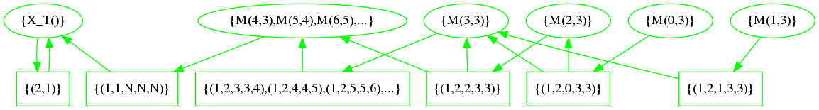
Figure 2: A part of the reduced dependency space where $M(x,y)$ holds.

Although a proof graph induced from the reduced dependency space is finite, the reduced dependency space is nevertheless useful because the search space is infinite. We also tried to solve a larger instance $a=10$ and got the spaces consisting of 394 nodes in 332 seconds, in which Z3 solver spent 325 seconds.

For another example, a disjunctive PBESs for a trading problem [16] is successfully solved by our implementation in a second, which produced a space consisting 12 nodes. Note that disjunctive PBESs is a subclass of existential PBESs.

In contrast, the procedure does not halt for the PBES $\mathcal{E}_{2}$ in Example 1, nor even for the next simple PBES:

$$\mu X(d{:}N)\,=\,(d=0)\vee(d>0\wedge X(d-1))$$

where its solution is $X=\mathbb{N}$. Our procedure starts from the entire set $\mathbb{N}$ and divides it into $\{0\}$ and $\{1,2,\dots\}$ because of the first clause. After that, the latter set is split into $\{1\}$ and $\{2,3,\dots\}$ using the second clause. Endlessly, the procedure splits the latter set into the minimum number and the others. From this observation, the feasibility condition on $\langle\sim_{D},\sim_{B}\rangle$ may be too strong, and weaker one is promising.

7 Conclusion

We have extended reduced dependency spaces for existential PBESs, and have shown that a proof graph is obtained from the space by solving parity games if the space is finite. Reduced dependency spaces are valuable because the dependency spaces for most of PBESs are infinite, but existential PBESs may have a finite reduced dependency space. We also have shown a procedure to construct reduced dependency spaces and have shown the correctness. We have shown some examples including a downsized McCarthy 91 function is successfully characterized by our method by applying an implementation.

Reduced dependency space is defined so that it contains all minimal proof graphs. For a membership problem to obtain a proof graph which proves $X({\bf v})$, a reduced space may require too many division to make the entire data domain consistent. This sometimes induces the loss of termination of the procedure. Proposing a more clever procedure is one of the future works. Moreover, our implementation relies on the shape of PBESs, not sets defined by them. This is indicated by the example in the last of section 6. To clarify these conditions is also our future works.

Appendix A Proof of Proposition 5

Definition 13

Existential PBESs are subclass of PBES defined by the following grammar:

$$\begin{array}[t]{rcl}\mathcal{E}&::=&\emptyset\ |\ \left(\nu X\left(d:D\right)=\varphi\right)\mathcal{E}\ |\ \left(\mu X\left(d:D\right)=\varphi\right)\mathcal{E}\\ \varphi&::=&b\ |\ \varphi\wedge\varphi\ |\ \varphi\vee\varphi\ |\ \exists d{:}D\ \varphi\ |\ X({\bf exp})\end{array}$$

The difference from the original definition is that the universal-quantifier does not occur in $\varphi$.

See 5

Proof A.14.

We can normalize each $\varphi$ by the following steps.

1. Rename all bound variables so that different scope variables are distinct.

2. Lift up all existential quantifiers to obtain the form $\exists{\bf e}{:}D.\ \varphi^{\prime}$.

3. Calculate the disjunctive normal form of $\varphi^{\prime}$ and obtain $\bigvee_{R}\varphi_{R}$. Then $\bigvee_{R}\exists{\bf e}{:}D.\ \varphi_{R}$ is an expected form.

$\sqcap$$\sqcup$

Appendix B Proofs related to proof graphs

B.1 Parity games and dependency spaces

Definition B.15.

A parity game is a directed graph $G=(V,{\to},\Omega,\Pi)$ such that

• $V$ is a set of vertices,

• ${\to}$ is a set of edges with ${\to}\subseteq V\times V$,

• $\Omega:V\to\mathbb{N}$ is a function which assigns priority to each vertex, and

• $\Pi:V\to\{\circ,\Box\}$ is a function which assigns player to each vertex.

Parity game is a game played by two players $\circ$ and $\Box$. This game progresses by moving the piece placed at a vertex along an edge. The player $\Pi(v)$ moves the piece when the piece is on a vertex $v$. We call a parity game started from $v$ if the piece is initially placed on the vertex $v$. A play of a parity game is a sequence of vertices that the piece goes through. The player $\circ$ wins the game if and only if the player $\Box$ cannot move the piece, or the largest priority that occurs infinitely often in the play is an even number when the play continues infinitely. We write $\mathrm{rank}^{\infty}(\pi)$ as this largest priority for the play $\pi$.

For a given parity game $G$ started from a fixed vertex, a strategy $S$ of a player is a function that selects a vertex to move along an edge, given a vertex owned by the player. A strategy $S$ is called a winning strategy when the player wins the game $G$ according to $S$ even if the opponent player plays optimally.

The next proposition shows the determinacy of the winner for parity games.

Proposition B.16 ([7]).

Given a parity game, starting vertex dominates the winner, which means that either of the player $\circ$ or $\Box$ has a winning strategy according to the vertex started from.

We say that a player wins the game on a vertex if he has a winning strategy started from the vertex.

A dependency space for a PBES $\mathcal{E}$ is regarded as a parity game. The function $\Pi$ naturally defined from the shape of $\vee$/$\wedge$-vertices, i.e., $\Pi(v)={\circ}$ if and only if $v$ is an $\vee$-vertex. We give the priority function $\Omega$ as follows:

$$\Omega(v)=\left\{\begin{array}[]{ll}u-\mathrm{rank}(X_{i}),&\text{if }v=X_{i}({\bf v})\in\mathrm{sig}(\mathcal{E})\\ 0,&\text{otherwise}\end{array}\right.$$

where $u$ is the minimum even number satisfying $u\geq\mathrm{rank}(X_{i})$ for any $X_{i}\in\mathrm{bnd}(\mathcal{E})$. We call this a parity game obtained from $\mathcal{E}$. Note that $V$ and ${\to}$ in dependency spaces are generally infinite sets, while $\{\Omega(v)\mid v\in V\}$ is finite. Thus each parity game corresponding to a dependency space is well-defined.

Moreover, a reduced dependency space obtained from a feasible relation ${\sim}$ is also regarded as a parity game, because $\Omega/{\sim}$ and $\Pi/{\sim}$ are well-defined. We call this a reduced parity game $G/{\sim}$ for a parity game $G$ and a feasible relation ${\sim}$.

B.2 Proof of Lemma 6

This lemma is justified by Lemma B.17.

Lemma B.17.

For a given PBES $\mathcal{E}$, there exists a proof graph that proves $X({\bf v}_{0})$ if and only if the player $\circ$ wins the game $G$, obtained from $\mathcal{E}$, on $X({\bf v}_{0})$.

Proof B.18.

We use the notation $X_{i}({\bf v})^{\bullet}$ to represent the postset of $X_{i}({\bf v})$ for the target graph.

$\Rightarrow$) Let $P$ be a proof graph of $X({\bf v}_{0})$. By the form of existential PBESs and the condition (1) of proof graphs, for every vertex $X_{i}({\bf v})$ in $P$ there exist $k$ and ${\bf w}$ such that

$$\varphi_{ik}({\bf v},{\bf w})\text{ and }X_{i}({\bf v})^{\bullet}\supseteq\\ \{X_{a_{ik1}}(f_{ik1}({\bf v},{\bf w})),\dots,X_{a_{ikp_{ik}}}(f_{ikp_{ik}}({\bf v},{\bf w}))\}.$$

From this, we take the strategy of the player $\circ$: when the piece is on a vertex $X_{i}({\bf v})\in P$, move the piece to $(i,k,{\bf v},{\bf w})$ for $k,{\bf w}$ determined by the above condition.

We show that the piece never goes on the $\vee$-vertices not in $P$ with the parity game started from $X({\bf v_{0}})$ by induction of the steps of the game. First, the piece is on $X({\bf v}_{0})$, and it is in $P$. Assume the piece is on $X_{i}({\bf v})\in P$. Let $(i,k,{\bf v},{\bf w})$ be the $\wedge$-vertex which the piece goes on under the strategy. From the definition of the strategy, all vertices to which the player $\Box$ can move the piece are in $P$. Thus, the piece never goes on the $\vee$-vertices not in $P$, and the strategy is well-defined.

We show that the strategy is winning strategy started from $X({\bf v}_{0})$. If the piece cannot move on a vertex $X_{i}({\bf v})$, then $\varphi_{ik}({\bf v},{\bf w})$ never holds for any $k,{\bf w}$ by the definition of $G$. Then, it contradicts the condition (1) of proof graphs. In addition, suppose that there exists an infinite parity game in which the player $\circ$ loses. Let $\pi$ be the infinite path tracing the movement of the piece. We define an infinite path $\pi^{\prime}$ from $\pi$ by collapsing the $\wedge$-vertices into $\vee$-vertices. Because $\pi^{\prime}$ only consists of $\vee$-vertices, $\pi^{\prime}$ is also a path of $P$. $P$ is a proof graph, therefore, the minimum rank of $X^{\infty}$ with $\pi^{\prime}$ is even by the condition (2) of proof graphs. In contrast, the largest priority on $\pi^{\prime}$ is odd because the player $\circ$ loses. The minimum rank with $\pi^{\prime}$ is odd by the definition of the priority function $\Omega$, however, this contradicts.

$\Leftarrow$) Assume that the player $\circ$ has a winning strategy. We construct a graph $P$:

• $X({\bf v}_{0})$ is in $P$.

• Suppose that $X_{i}({\bf v})$ is in $P$ and $(i,k,{\bf v},{\bf w})$ is the vertex to which the player $\circ$ moves the piece on $X_{i}({\bf v})$. Then, $(i,k,{\bf v},{\bf w})^{\bullet}$ is in $P$ and there exist edges from $X_{i}({\bf v})$ to each vertex in $(i,k,{\bf v},{\bf w})^{\bullet}$.

It is obvious that the graph $P$ have the conditions of proof graphs.     $\sqcap$$\sqcup$

B.3 Proof of Theorem 9

Proposition B.19.

Let $G$ be a parity game and $G/{\sim}$ be a reduced parity game for a PBES. Then, for all vertex $[A]_{\sim},[B]_{\sim}\in G/{\sim}$ and for all $u\in[A]_{\sim}$, $[A]_{\sim}\to[B]_{\sim}$ implies $\exists v\in[B]_{\sim}.\ u\to v$.

The theorem 9 holds immediate from the following lemma and the fact that solving a finite parity game is decidable.

Lemma B.20.

The player $\circ$ wins on $X({\bf v})$ for a dependency space if and only if the player $\circ$ wins on $[X({\bf v})]_{\sim}$ for a reduced dependency space.

Proof B.21.

$\Rightarrow$) We prove contraposition. Suppose the player $\circ$ loses on $[X({\bf v})]_{\sim}$. This means that the player $\Box$ wins on $[X({\bf v})]_{\sim}$ by the proposition B.16. Let $S^{\prime}$ be a winning strategy of the player $\Box$ on $[X({\bf v})]_{\sim}$. Then, a strategy $S$ of the player $\Box$ on $X({\bf v})$ can be defined as $S(u)=v$ for $u\in G$ where $v\in S^{\prime}([u]_{\sim})$ from the proposition B.19.

Any game $P$ on $X({\bf v})$ according to the strategy $S$ is corresponding to a game $P^{\prime}$ on $[X({\bf v})]_{\sim}$ according to the strategy $S^{\prime}$. That is, the sequence of the rank $P$ is equal to the sequence of $P^{\prime}$. $S^{\prime}$ is a winning strategy, therefore $S$ is also a winning strategy.

$\Leftarrow$) Suppose the player $\circ$ has a winning strategy $S^{\prime}$ on $[X({\bf v})]_{\sim}$. We can define a strategy $S$ on $X({\bf v})$ using $S^{\prime}$ in a similar way, and $S$ is also a winning strategy.     $\sqcap$$\sqcup$

B.4 Proof of Theorem 12

See 12

Proof B.22.

Proof by contradiction. Let $\mathcal{P}=\langle\dots,\Phi_{i}^{\infty},\dots,\Psi_{ik}^{\infty},\dots\rangle$ be a fixed-point of $H$ and ${\sim_{\mathcal{P}}}={\sim_{\mathcal{P}}^{D}}\cup{\sim_{\mathcal{P}}^{B}}$. If $\mathcal{P}$ is not feasible, then at least one of the following conditions holds:

1. There exists $X_{i}({\bf v})$ and $X_{i}({\bf v}^{\prime})$ such that $X_{i}({\bf v})\sim_{\mathcal{P}}X_{i}({\bf v}^{\prime})$ and $F_{ik}(X_{i}({\bf v}))\not\sim_{\mathcal{P}}F_{ik}(X_{i}({\bf v}^{\prime}))$ for some $k$.

2. There exists $(i,k,{\bf v},{\bf w})$ and $(i,k,{\bf v^{\prime}},{\bf w^{\prime}})$ such that $(i,k,{\bf v},{\bf w})\sim_{\mathcal{P}}(i,k,{\bf v^{\prime}},{\bf w^{\prime}})$ and $G_{ik}(i,k,{\bf v},{\bf w})\not\sim_{\mathcal{P}}G_{ik}(i,k,{\bf v^{\prime}},{\bf w^{\prime}})$.

Suppose the condition (1) holds. Then, w.l.o.g., $\bigcup_{x\in F_{ik}(X_{i}({\bf v^{\prime}}))}[x]_{\sim_{\mathcal{P}}}\cap[(i,k,{\bf v},{\bf w})]_{\sim_{\mathcal{P}}}=\emptyset$ for some $(i,k,{\bf v},{\bf w}){\hskip 0.3pt\in}$ $F_{ik}(X_{i}({\bf v}))$ by the definition of feasible relation. In particular, because $\bigcup_{x\in F_{ik}(X_{i}({\bf v^{\prime}}))}[x]_{\sim_{\mathcal{P}}}\supseteq F_{ik}(X_{i}({\bf v^{\prime}}))$, $F_{ik}(X_{i}({\bf v^{\prime}}))\cap[(i,k,{\bf v},{\bf w})]_{\sim_{\mathcal{P}}}=\emptyset$. Let $\psi=[(i,k,{\bf v},{\bf w})]_{\sim_{\mathcal{P}}}\in\Psi_{ik}^{\infty}$. We have $F_{ik}(X_{i}({\bf v}))\cap\psi\supseteq\{(i,k,{\bf v},{\bf w})\}\not=\emptyset$ and $F_{ik}(X_{i}({\bf v^{\prime}}))\cap\psi=\emptyset$. Therefore, $X_{i}({\bf v})$ and $X_{i}({\bf v^{\prime}})$ belong different block when ${\otimes_{ik}^{D}}$ splits $\mathcal{P}$. This contradicts that $\mathcal{P}$ is a fixed-point of $H$.

Moreover, suppose the condition (2) holds. By a similar argument, there exists $X_{a}(d_{a})\in G_{ik}(i,k,{\bf v},{\bf w})$ such that $G_{ik}(i,k,{\bf v^{\prime}},{\bf w^{\prime}})\cap[X_{a}(d_{a})]_{\sim_{\mathcal{P}}}=\emptyset$. Recall $G_{ik}(i,k,{\bf v},{\bf w})=\{X_{a_{1}}(f_{1}({\bf v},{\bf w})),\dots,X_{a_{p}}(f_{p}({\bf v},{\bf w}))\}$, $a=a_{q}$ and $d_{a}=f_{q}({\bf v},{\bf w})$ for some $1\leq q\leq p$. Let $\phi=[X_{a}(d_{a})]_{\sim_{\mathcal{P}}}\in\Phi_{a}$. Obviously, $G_{ik}(i,k,{\bf v},{\bf w})\cap\phi\not=\emptyset$ and $G_{ik}(i,k,{\bf v^{\prime}},{\bf w^{\prime}})\cap\phi=\emptyset$. Thus, $(i,k,{\bf v},{\bf w})$ and $(i,k,{\bf v^{\prime}},{\bf w^{\prime}})$ belong different block when ${\otimes_{ik}^{B}}$ splits $\mathcal{P}$. This contradicts $\mathcal{P}$ is a fixed-point.     $\sqcap$$\sqcup$

References

• [1]
• [2] T. Chen, B. Ploeger, J. van de Pol & T. A. C. Willemse (2007): Equivalence Checking for Infinite Systems Using Parameterized Boolean Equation Systems. In: Proceedings of the 18th International Conference on Concurrency Theory (CONCUR’07), LNCS 4703, Springer, Berlin, Heidelberg, pp. 120–135, 10.1007/978-3-540-74407-8_9.
• [3] E. Clarke, O. Grumberg, S. Jha, Y. Lu & H. Veith (2003): Counterexample-guided Abstraction Refinement for Symbolic Model Checking. Journal of ACM 50(5), pp. 752–794, 10.1145/876638.876643.
• [4] E. M. Clarke, Jr., O. Grumberg & D. A. Peled (1999): Model Checking. MIT Press, Cambridge, MA, USA.
• [5] S. Cranen, B. Luttik & T. A. C. Willemse (2013): Proof Graphs for Parameterised Boolean Equation Systems. In: Proc. of the 24th International Conference on Concurrency Theory, (CONCUR 2013), LNCS 8052, Springer, pp. 470–484, 10.1007/978-3-642-40184-8_33.
• [6] L. De Moura & N. Bjørner (2008): Z3: An Efficient SMT Solver. In: Proc. of the 14th International Conference on Tools and Algorithms for the Construction and Analysis of Systems (TACAS’08), LNCS 4963, Springer, Berlin, Heidelberg, pp. 337–340, 10.1007/978-3-540-78800-3_24.
• [7] E. A. Emerson & C. S. Jutla (1991): Tree automata, mu-calculus and determinacy. In: Foundations of Computer Science, 1991. Proceedings, 32nd Annual Symposium on, IEEE, pp. 368–377, 10.1109/SFCS.1991.185392.
• [8] O. Friedmann & M. Lange (2017): The PGSolver Collection of Parity Game Solvers. Available at https://github.com/tcsprojects/pgsolver/blob/master/doc/pgsolver.pdf.
• [9] E. Grädel, P. G. Kolaitis, L. Libkin, M. Marx, J. Spencer, M. Y. Vardi, Y. Venema & S. Weinstein (2007): Finite Model Theory and Its Applications. Texts in Theoretical Computer Science. An EATCS Series, Springer, 10.1007/3-540-68804-8.
• [10] S. Graf & H. Saidi (1997): Construction of Abstract State Graphs with PVS. In: Proc. of the 9th International Conference Computer Aided Verification (CAV’97), LNCS 1254, Springer, pp. 72–83, 10.1007/3-540-63166-6_10.
• [11] J. F. Groote & T. Willemse (2004): Parameterised Boolean Equation Systems. In: Proc. of 15th International Conference on Concurrency Theory (CONCUR 2004), LNCS 3170, Springer, pp. 308–324, 10.1007/978-3-540-28644-8_20.
• [12] J. F. Groote & T. A. C. Willemse (2005): Model-checking Processes with Data. Science of Computer Programming 56(3), pp. 251–273, 10.1016/j.scico.2004.08.002.
• [13] J. F. Groote & T. A. C. Willemse (2005): Parameterised Boolean Equation Systems. Theoretical Computer Science 343(3), pp. 332–369, 10.1016/j.tcs.2005.06.016.
• [14] J. F. Groote & T. A. C. Willemse (2004): A Checker for Modal Formulae for Processes with Data. In: Proc. of the 2nd International Symposium on Formal Methods for Components and Objects (FMCO 2003), LNCS 3188, Springer, pp. 223–239, 10.1007/978-3-540-30101-1_10.
• [15] R. P. J. Koolen, T. A. C. Willemse & H. Zantema (2015): Using SMT for Solving Fragments of Parameterised Boolean Equation Systems. In: Proc. of the 13th International Symposium on Automated Technology for Verification and Analysis (ATVA 2015), LNCS 9364, Springer, pp. 14–30, 10.1007/978-3-319-24953-7_3.
• [16] Y. Nagae, M. Sakai & H. Seki (2017): An Extension of Proof Graphs for Disjunctive Parameterised Boolean Equation Systems. Electronic Proceedings in Theoretical Computer Science 235, pp. 46–61, 10.4204/EPTCS.235.4.
• [17] S. Orzan, W. Wesselink & T. A. C. Willemse (2009): Static Analysis Techniques for Parameterised Boolean Equation Systems. In: Proc. of the 15th International Conference on Tools and Algorithms for the Construction and Analysis of Systems (TACAS 2009), LNCS 5505, Springer, pp. 230–245, 10.1007/978-3-642-00768-2_22.
• [18] B. Ploeger, J. W. Wesselink & T. A. C. Willemse (2011): Verification of Reactive Systems via Instantiation of Parameterised Boolean Equation Systems. Information and Computation 209(4), pp. 637–663, 10.1016/j.ic.2010.11.025.
• [19] M. Presburger (1929): Über die Vollständigkeit eines gewissen Systems der Arithmetik ganzer Zahlen. In: welchem die Addition als einzige Operation hervortritt, C. R. ler congrès des Mathématiciens des pays slaves, Warszawa, pp. 92–101.