Efficient Implementation of Evaluation Strategies
via Token-Guided Graph Rewriting

Abstract

In implementing evaluation strategies of the lambda-calculus, both correctness and efficiency of implementation are valid concerns. While the notion of correctness is determined by the evaluation strategy, regarding efficiency there is a larger design space that can be explored, in particular the trade-off between space versus time efficiency. We contributed to the study of this trade-off by the introduction of an abstract machine for call-by-need, inspired by Girard’s Geometry of Interaction, a machine combining token passing and graph rewriting. This work presents an extension of the machine, to additionally accommodate left-to-right and right-to-left call-by-value strategies. We show soundness and completeness of the extended machine with respect to each of the call-by-need and two call-by-value strategies. Analysing time cost of its execution classifies the machine as “efficient” in Accattoli’s taxonomy of abstract machines.

1 Introduction

The lambda-calculus is a simple yet rich model of computation, relying on a single mechanism to activate a function in computation, beta-reduction, that replaces function arguments with actual input. While in the lambda-calculus itself beta-reduction can be applied in an unrestricted way, it is evaluation strategies that determine the way beta-reduction is applied when the lambda-calculus is used as a programming language. Evaluation strategies often imply how intermediate results are copied, discarded, cached or reused. For example, everything is repeatedly evaluated as many times as requested in the call-by-name strategy. In the call-by-need strategy, once a function requests its input, the input is evaluated and the result is cached for later use. The call-by-value strategy evaluates function input and caches the result even if the function does not require the input.

The implementation of any evaluation strategy must be correct, first of all, i.e. it has to produce results as stipulated by the strategy. Once correctness is assured, the next concern is efficiency. One may prefer better space efficiency, or better time efficiency, and it is well known that one can be traded off for the other. For example, time efficiency can be improved by caching more intermediate results, which increases space cost. Conversely, bounding space requires repeating computations, which adds to the time cost. Whereas correctness is well defined for any evaluation strategy, there is a certain freedom in managing efficiency. The challenge here is how to produce a unified framework which is flexible enough to analyse and guide the choices required by this trade-off. Recent studies by Accattoli et al. [5, 3, 2] clearly establish classes of efficiency for a given evaluation strategy. They characterise efficiency by means of the number of beta-reduction applications required by the strategy, and introduce two efficiency classes, namely “efficient” and “reasonable.” The expected efficiency of an abstract machine gives us a starting point to quantitatively analyse the trade-offs required in an implementation.

We employ Girard’s Geometry of Interaction (GoI) [16], a semantics of linear logic proofs, as a framework for studying the trade-off between time and space efficiency. In particular we focus on GoI-style abstract machines for the lambda-calculus, pioneered by Danos and Regnier [9] and Mackie [20]. These machines evaluate a term of the lambda-calculus by translating the term to a graph, a network of simple transducers, which executes by passing a data-carrying token around.

The token simulates graph rewriting without actually rewriting, which is in fact a particular instance of the trade-off we mentioned above. The token-passing machines keep the underlying graph fixed and use the data stored in the token to route it. They therefore favour space efficiency at the cost of time efficiency. The same computation is repeated when, instead, intermediate results could have been cached by saving copies of certain sub-graphs representing values.

Our intention is to lift the GoI-style token passing to a framework to analyse the trade-off of efficiency, by strategically interleaving it with graph rewriting. The key idea is that the token holds control over graph rewriting, by visiting redexes and triggering rewrite rules. Graph rewriting offers fine control over caching and sharing intermediate results, however fetching cached results can increase the size of the graph. In short, introduction of graph rewriting sacrifices space while favouring time efficiency. We expect the flexibility given by a fine-grained control over interleaving will enable a careful balance between space and time efficiency.

This idea was first introduced in our previous work [23], by developing an abstract machine that interleaves token passing with as much graph rewriting as possible. We showed the resulting graph-rewriting abstract machine implements call-by-need evaluation, and it is classified as “efficient” in terms of time. We further develop this idea by proposing an extension of the graph-rewriting abstract machine, to accommodate other evaluation strategies, namely left-to-right and right-to-left call-by-value. In our framework, both call-by-value strategies involve similar tactics for caching intermediate results as the call-by-need strategy, with the only difference being the timing of cache creation.

Contributions. We extend the token-guided graph-rewriting abstract machine for the call-by-need strategy [23] to the left-to-right and right-to-left call-by-value strategies. The presentation of the machine is revised by using term graphs instead of proof nets [15], to make clearer sense of evaluation strategies in the graphical representation of terms. The extension is by introducing nodes that correspond to different evaluation strategies, rather than modifying the behaviour of existing nodes to suite different evaluation strategy demands. We prove the soundness and completeness of the extended machine with respect to the three evaluation strategies separately, using a “sub-machine” semantics, where the word ‘sub’ indicates both a focus on substitution and its status as an intermediate representation. The sub-machine semantics is based on Sinot’s “token-passing” semantics [27, 28] that makes explicit the two main tasks of abstract machines: searching redexes and substituting variables. The time-cost analysis classifies the machine as “efficient” in Accattoli’s taxonomy of abstract machines [2]. Finally, an on-line visualiser is implemented, in which the machine can be executed on arbitrary closed lambda-terms.

2 A Term Calculus with Sub-Machine Semantics

We use an untyped term calculus that accommodates three evaluation strategies of the lambda-calculus, by dedicated constructors for function application: namely, $\mathbin{@}$ (call-by-need), $\mathbin{\overrightarrow{@}}$ (left-to-right call-by-value) and $\mathbin{\overleftarrow{@}}$ (right-to-left call-by-value). The term calculus uses all strategies so that we do not have to present three almost identical calculi. But we are not interested in their interaction, but in each strategy separately. In the rest of the paper, we therefore assume that each term contains function applications of a single strategy. As shown in the top of Fig. 1, the calculus accommodates explicit substitutions $[x\leftarrow u]$. A term with no explicit substitutions is said to be “pure.”

The sub-machine semantics is used to establish the soundness of the graph-rewriting abstract machine. It is an adaptation of Sinot’s lambda-term rewriting system [27, 28], used to analyse a token-guided rewriting system for interaction nets. It imitates an abstract machine by explicitly searching for a redex and decomposing the meta-level substitution into on-demand linear substitution, also resembling a storeless abstract machine (e.g. [10, Fig. 8]). However the semantics is still too “abstract” as an abstract machine, in the sense that it works modulo alpha-equivalence to avoid variable captures.

Fig. 1 defines the sub-machine semantics of our calculus. It is given by labelled relations between enriched terms $E\langle\llparenthesis t\rrparenthesis\rangle$. In an enriched term $E\langle\llparenthesis t\rrparenthesis\rangle$, a sub-term $t$ is not plugged directly into the evaluation context, but into a “window” $\llparenthesis\cdot\rrparenthesis$ which makes it syntactically obvious where the reduction context is situated. Forgetting the window turns an enriched term into an ordinary term. Basic rules $\mapsto$ are labelled with $\beta$, $\sigma$ or $\epsilon$. The basic rules (2), (5) and (8), labelled with $\beta$, apply beta-reduction and delay substitution of a bound variable. Substitution is done one by one, and on demand, by the basic rule (10) with label $\sigma$. Each application of the basic rule (10) replaces exactly one bound variable with a value, and keeps a copy of the value for later use. All other basic rules, with label $\epsilon$, search for a redex by moving the window without changing the underlying term. Finally, reduction is defined by congruence of basic rules with respect to evaluation contexts, and labelled accordingly. Any basic rules and reductions are indeed between enriched terms, because the window $\llparenthesis\cdot\rrparenthesis$ is never duplicated or discarded.

$$t,u ::=x\mid\lambda{x}.t\mid t\mathbin{@}u\mid t\mathbin{\overrightarrow{@}}u\mid t\mathbin{\overleftarrow{@}}u\mid t[x\leftarrow u],\quad v::=\lambda{x}.t$$ (terms, values)

$$A ::=\langle\cdot\rangle\mid A[x\leftarrow t]$$ (answer contexts)

$$E ::=\langle\cdot\rangle\mid E\mathbin{@}t\mid E\mathbin{\overrightarrow{@}}t\mid A\langle v\rangle\mathbin{\overrightarrow{@}}E\mid t\mathbin{\overleftarrow{@}}E\mid E\mathbin{\overleftarrow{@}}A\langle v\rangle\mid E[x\leftarrow t]\mid E\langle x\rangle[x\leftarrow E]$$ (evaluation contexts)

Basic rules $\mapsto_{\_}\beta$, $\mapsto_{\_}\sigma$ and $\mapsto_{\_}\epsilon$:
$\displaystyle\llparenthesis t\mathbin{@}u\rrparenthesis$ $\displaystyle\mapsto_{\_}\epsilon\llparenthesis t\rrparenthesis\mathbin{@}u$ (1) $\displaystyle A\langle\llparenthesis\lambda{x}.t\rrparenthesis\rangle\mathbin{@}u$ $\displaystyle\mapsto_{\_}\beta A\langle\llparenthesis t\rrparenthesis[x\leftarrow u]\rangle$ (2) $\displaystyle\llparenthesis t\mathbin{\overrightarrow{@}}u\rrparenthesis$ $\displaystyle\mapsto_{\_}\epsilon\llparenthesis t\rrparenthesis\mathbin{\overrightarrow{@}}u$ (3) $\displaystyle A\langle\llparenthesis\lambda{x}.t\rrparenthesis\rangle\mathbin{\overrightarrow{@}}u$ $\displaystyle\mapsto_{\_}\epsilon A\langle\lambda{x}.t\rangle\mathbin{\overrightarrow{@}}\llparenthesis u\rrparenthesis$ (4) $\displaystyle A\langle\lambda{x}.t\rangle\mathbin{\overrightarrow{@}}A^{\prime}\langle\llparenthesis v\rrparenthesis\rangle$ $\displaystyle\mapsto_{\_}\beta A\langle\llparenthesis t\rrparenthesis[x\leftarrow A^{\prime}\langle v\rangle]\rangle$ (5) $\displaystyle\llparenthesis t\mathbin{\overleftarrow{@}}u\rrparenthesis$ $\displaystyle\mapsto_{\_}\epsilon t\mathbin{\overleftarrow{@}}\llparenthesis u\rrparenthesis$ (6) $\displaystyle t\mathbin{\overleftarrow{@}}A\langle\llparenthesis v\rrparenthesis\rangle$ $\displaystyle\mapsto_{\_}\epsilon\llparenthesis t\rrparenthesis\mathbin{\overleftarrow{@}}A\langle v\rangle$ (7) $\displaystyle A\langle\llparenthesis\lambda{x}.t\rrparenthesis\rangle\mathbin{\overleftarrow{@}}A^{\prime}\langle v\rangle$ $\displaystyle\mapsto_{\_}\beta A\langle\llparenthesis t\rrparenthesis[x\leftarrow A^{\prime}\langle v\rangle]\rangle$ (8) $\displaystyle E\langle\llparenthesis x\rrparenthesis\rangle[x\leftarrow A\langle u\rangle]$ $\displaystyle\mapsto_{\_}\epsilon E\langle x\rangle[x\leftarrow A\langle\llparenthesis u\rrparenthesis\rangle]$ (9) $\displaystyle E\langle x\rangle[x\leftarrow A\langle\llparenthesis v\rrparenthesis\rangle]$ $\displaystyle\mapsto_{\_}\sigma A\langle E\langle\llparenthesis v\rrparenthesis\rangle[x\leftarrow v]\rangle$ (10)

Reductions $\multimap_{\_}\beta$, $\multimap_{\_}\sigma$ and $\multimap_{\_}\epsilon$:    $E\langle\tilde{t}\rangle\multimap_{\_}\chi E\langle\tilde{u}\rangle\tilde{t}\mapsto_{\_}\chi\tilde{u}$

Figure 1: ”Sub-Machine” Operational Semantics

An evaluation of a pure term $t$ (i.e. a term with no explicit substitution) is a sequence of reductions starting from $\langle\llparenthesis t\rrparenthesis\rangle$, which is simply $\llparenthesis t\rrparenthesis$. In any evaluation, a sub-term in the window $\llparenthesis\cdot\rrparenthesis$ is always pure.

3 Token-Guided Graph-Rewriting Machine

A graph is given by a set of nodes and a set of directed edges. Nodes are classified into proper nodes and link nodes. Each edge is directed, and at least one of its two endpoints is a link node. An interface of a graph is given by two sets of link nodes, namely input and output. Each link node is a source of at most one edge, and a target of at most one edge. Input links are the only links that are not a target of any edge, and output links are the only ones that are not a source of any edge. When a graph $G$ has $n$ input link nodes and $m$ output link nodes, we sometimes write $G(n,m)$ to emphasise its interface. If a graph has exactly one input, we refer to the input link node as “root.”

The idea of using link nodes, as distinguished from proper nodes, comes from a graphical formalisation of string diagrams [18]. String diagrams consist of “boxes” that are connected to each other by “wires.” In the formalisation, boxes are modelled by “box-vertices” (corresponding to proper nodes in our case), and wires are modelled by consecutive edges connected via “wire-vertices” (corresponding to link nodes in our case). The segmentation of wires into edges can introduce an arbitrary number of consecutive link nodes, however these consecutive link nodes are identified by the notion of “wire homeomorphism.” We will later discuss these consecutive link nodes, from the perspective of the graph-rewriting machine. From now on we simply call a proper node “node,” and a link node “link.”

In drawing graphs, we follow the convention that input links are placed at the bottom and output links are at the top, and links are usually not drawn explicitly. The latter point means that edges are simply drawn from a node to a node, with intermediate links omitted. In particular if an edge is connected to an interface link, the edge is drawn as an open edge missing an endpoint. Additionally, we use a bold-stroke edge/node to represent a bunch of parallel edges/nodes.

Nodes are labelled, and a node with a label $X$ is called an “$X$-node.” We use two sorts of labels. One sort corresponds to the constructors of the calculus presented in Sec. 2, namely $\lambda$ (abstraction), $\mathbin{@}$ (call-by-need application), $\mathbin{\overrightarrow{@}}$ (left-to-right call-by-value application) and $\mathbin{\overleftarrow{@}}$ (right-to-left call-by-value application). These three application nodes are the novelty of this work. The token, travelling in a graph, reacts to these nodes in different ways, and hence implements different evaluation orders. We believe that this is a more extensible way to accommodate different evaluation orders, than to let the token react to the same node in different ways depending on situation. The other sort consists of $\mathop{!}$, $\wn$, $\mathit{D}$ and $\mathit{C}_{\_}n$ for any natural number $n$, used in the management of copying sub-graphs. This sort is inspired by proof nets of the multiplicative and exponential fragment of linear logic [15], and $\mathit{C}_{\_}n$-nodes generalise the standard binary contraction and incorporate weakening.

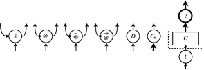
Figure 2: Graph Nodes

The number of input/output and incoming/outgoing edges for a node is determined by the label, as indicated in Fig. 2. We distinguish two outputs of an application node ($\mathbin{@}$, $\mathbin{\overrightarrow{@}}$ or $\mathbin{\overleftarrow{@}}$), calling one “composition output” and the other “argument output” (cf. [6]). A bullet $\bullet$ in the figure specifies a function output. The dashed box indicates a sub-graph $G(1,m)$ (“$\mathop{!}$-box”) that is connected to one $\mathop{!}$-node (“principal door”) and $m$ $\wn$-nodes (“auxiliary doors”). This $\mathop{!}$-box structure, taken from proof nets, aids duplication of sub-graphs by specifying those that can be copied.

We define a graph-rewriting abstract machine as a labelled transition system between graph states.

Definition 3.1 (Graph states).

A graph state $((G(1,0),e),\delta)$ is formed of a graph $G(1,0)$ with its distinguished link $e$, and token data $\delta=(d,f,S,B)$ that consists of: a direction defined by $d::=\mathord{\uparrow}\mid\mathord{\downarrow}$, a rewrite flag defined by $f::=\square\mid\lambda\mid\mathop{!}$, a computation stack defined by $S::=\square\mid\star:S\mid\lambda:S\mid@:S$, and a box stack defined by $B::=\square\mid\star:B\mid\mathop{!}:B\mid\diamond:B\mid e^{\prime}:B$, where $e^{\prime}$ is any link of the graph $G$.

The distinguished link $e$ is called the “position” of the token. The token reacts to a node in a graph using its data, which determines its path. Given a graph $G$ with root $e_{\_}0$, the initial state $\mathit{Init}(G)$ on it is given by $((G,e_{\_}0),(\mathord{\uparrow},\square,\square,\star:\square))$, and the final state $\mathit{Final}(G)$ on it is given by $((G,e_{\_}0),(\mathord{\downarrow},\square,\square,\mathop{!}:\square))$. An execution on a graph $G$ is a sequence of transitions starting from the initial state $\mathit{Init}(G)$.

Each transition $((G,e),\delta)\to_{\_}\chi((G^{\prime},e^{\prime}),\delta^{\prime})$ between graph states is labelled by either $\beta$, $\sigma$ or $\epsilon$. Transitions are deterministic, and classified into pass transitions that search for redexes and trigger rewriting, and rewrite transitions that actually rewrite a graph as soon as a redex is found.

A pass transition $((G,e),(d,\square,S,B))\to_{\_}\epsilon((G,e^{\prime}),(d^{\prime},f^{\prime},S^{\prime},B^{\prime}))$, always labelled with $\epsilon$, applies to a state whose rewrite flag is $\square$. It simply moves the token over one node, and updates its data by modifying the top elements of stacks, while keeping an underlying graph unchanged. When the token passes a $\lambda$-node or a $\mathop{!}$-node, a rewrite flag is changed to $\lambda$ or $\mathop{!}$, which triggers rewrite transitions. Fig. 3 defines pass transitions, by showing only the relevant node for each transition. The position of the token is drawn as a black triangle, pointing towards the direction of the token. In the figure, $X\neq\star$, and $n$ is a natural number. The pass transition over a $\mathit{C}_{\_}{n+1}$-node pushes the old position $e$, a link node, to a box stack.

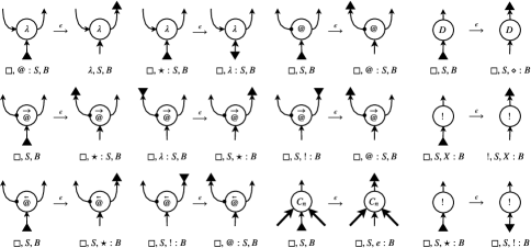
Figure 3: Pass Transitions

The way the token reacts to application nodes ($\mathbin{@}$, $\mathbin{\overrightarrow{@}}$ and $\mathbin{\overleftarrow{@}}$) corresponds to the way the window $\llparenthesis\cdot\rrparenthesis$ moves in evaluating these function applications in the sub-machine semantics (Fig. 1). When the token moves on to the composition output of an application node, the top element of a computational stack is either $@$ or $\star$. The element $\star$ makes the token return from a $\lambda$-node, which corresponds to reducing the function part of application to a value (i.e. abstraction). The element $@$ lets the token proceed at a $\lambda$-node, raises the rewrite flag $\lambda$, and hence triggers a rewrite transition that corresponds to beta-reduction. The call-by-value application nodes ($\mathbin{\overrightarrow{@}}$ and $\mathbin{\overleftarrow{@}}$) send the token to their argument output, pushing the element $\star$ to a box stack. This makes the token bounce at a $\mathop{!}$-node and return to the application node, which corresponds to evaluating the argument part of function application to a value. Finally, pass transitions through $\mathit{D}$-nodes, $\mathit{C}_{\_}n$-nodes and $\mathop{!}$-nodes prepare copying of values, and eventually raise the rewrite flag $\mathop{!}$ that triggers on-demand duplication.

A rewrite transition $((G,e),(d,f,S,B))\to_{\_}\chi((G^{\prime},e^{\prime}),(d^{\prime},f^{\prime},S,B^{\prime}))$, labelled with $\chi\in\{\beta,\sigma,\epsilon\}$, applies to a state whose rewrite flag is either $\lambda$ or $\mathop{!}$. It changes a specific sub-graph while keeping its interface, changes the position accordingly, and pops an element from a box stack. Fig. 4 defines rewrite transitions by showing a sub-graph (“redex”) to be rewritten. Before we go through each rewrite transition, we note that rewrite transitions are not exhaustive in general, as a graph may not match a redex even though a rewrite flag is raised. However we will see that there is no failure of transitions in implementing the term calculus.

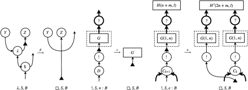
Figure 4: Rewrite Transitions

The first rewrite transition in Fig. 4, with label $\beta$, occurs when a rewrite flag is $\lambda$. It implements beta-reduction by eliminating a pair of an abstraction node ($\lambda$) and an application node ($\$\in\{\mathbin{@},\mathbin{\overrightarrow{@}},\mathbin{\overleftarrow{@}}\}$ in the figure). Outputs of the $\lambda$-node are required to be connected to arbitrary nodes (labelled with $Y$ and $Z$ in the figure), so that edges between links are not introduced. The other rewrite transitions are for the rewrite flag $\mathop{!}$, and they together realise the copying process of a sub-graph (namely a $\mathop{!}$-box). The second rewrite transition in Fig. 4, labelled with $\epsilon$, finishes off each copying process by eliminating all doors of the $\mathop{!}$-box $G$. It replaces the interface of $G$ with output links of the auxiliary doors and the input link of the $\mathit{D}$-node, which is the new position of the token, and pops the top element $\diamond$ of a box stack. Again, no edge between links are introduced.

The last rewrite transition in the figure, with label $\sigma$, actually copies a $\mathop{!}$-box. It requires the top element $e$ of the old box stack to be one of input links of the $\mathit{C}_{\_}{k+1}$-node (where $k$ is a natural number). The link $e$ is popped from the box stack and becomes the new position of the token, and the $\mathit{C}_{\_}{k+1}$-node becomes a $\mathit{C}_{\_}k$-node by keeping all the inputs except for the link $e$. The sub-graph $H(n+m,l)$ consists of $l$ parallel $\mathit{C}$-nodes that altogether have $n+m$ inputs. Among these inputs, $n$ are connected to auxiliary doors of the $\mathop{!}$-box $G(1,n)$, and $m$ are connected to nodes that are not in the redex. The sub-graph $H(n+m,l)$ is turned into $H^{\prime}(2n+m,l)$ by introducing $n$ inputs to these $\mathit{C}$-nodes as follows: if an auxiliary door of the $\mathop{!}$-box $G$ is connected to a $\mathit{C}$-node in $H$, two copies of the auxiliary door are both connected to the corresponding $\mathit{C}$-node in $H^{\prime}$. Therefore the two sub-graphs consist of the same number $l$ of $\mathit{C}$-nodes, whose indegrees are possibly increased. The $m$ inputs, connected to nodes outside a redex, are kept unchanged. For example, copying a graph $G(1,3)$ for $H(5,2)$ will give an $H^{\prime}(8,2)$ as shown above.

All pass and rewrite transitions are well-defined. The following “sub-graph” property is essential in time-cost analysis, because it bounds the size of duplicable sub-graphs (i.e. $\mathop{!}$-boxes) in an execution.

Lemma 3.2 (Sub-graph property).

For any execution $\mathit{Init}(G)\to^{*}\mathit{Final}((H,e),\delta)$, each $\mathop{!}$-box of the graph $H$ appears as a sub-graph of the initial graph $G$.

Proof.

Rewrite transitions can only copy or discard a $\mathop{!}$-box, and cannot introduce, expand or reduce a single $\mathop{!}$-box. Therefore, any $\mathop{!}$-box of $H$ has to be already a $\mathop{!}$-box of the initial graph $G$. ∎

When a graph has an edge between links, the token is just passed along. With this pass transition over a link at hand, the equivalence relation between graphs that identifies consecutive links with a single link—so-called “wire homeomorphism” [18]—lifts to a weak bisimulation between graph states. Therefore, behaviourally, we can safely ignore consecutive links. From the perspective of time-cost analysis, we benefit from the fact that rewrite transitions are designed not to introduce any edge between links. This means, by assuming that an execution starts with a graph with no consecutive links, we can analyse time cost of the execution without caring the extra pass transition over a link.

4 Implementation of Evaluation Strategies

The implementation of the term calculus, by means of the dynamic GoI, starts with translating (enriched) terms into graphs. The definition of the translation uses multisets of variables, to track how many times each variable occurs in a term. We assume that terms are alpha-converted in a form in which all binders introduce distinct variables.

Notation (Multiset).

The empty multiset is denoted by $\emptyset$, and the sum of two multisets $M$ and $M^{\prime}$ is denoted by $M+M^{\prime}$. We write $x\in^{k}M$ if the multiplicity of $x$ in a multiset $M$ is $k$. Removing all $x$ from a multiset $M$ yields the multiset $M\backslash x$, e.g. ${[x,x,y]\backslash x}=[y]$. We abuse the notation and refer to a multiset $[x,\ldots,x]$ of a finite number of $x$’s, simply as $x$.

Definition 4.1 (Free variables).

The map $\mathit{FV}$ of terms to multisets of variables is inductively defined by:

$$\mathit{FV}(x) :=[x], \mathit{FV}(\lambda{x}.t) :=\mathit{FV}(t)\backslash x,$$

$$\mathit{FV}(t\mathbin{\$}u) :=\mathit{FV}(t)+\mathit{FV}(u), \mathit{FV}(t[x\leftarrow u]) :=(\mathit{FV}(t)\backslash x)+\mathit{FV}(u). \mathbin{\$}\in\{\mathbin{@},\mathbin{\overrightarrow{@}},\mathbin{\overleftarrow{@}}\}$$ ()

For a multiset $M$ of variables, the map $\mathit{FV}_{\_}M$ of evaluation contexts to multisets of variables is defined by:

$$\mathit{FV}_{\_}M(\langle\cdot\rangle) :=M, \mathit{FV}_{\_}M(t\mathbin{\overleftarrow{@}}E) :=\mathit{FV}(t)+\mathit{FV}_{\_}M(E),$$

$$\mathit{FV}_{\_}M(E\mathbin{@}t) :=\mathit{FV}_{\_}M(E)+\mathit{FV}(t), \mathit{FV}_{\_}M(E\mathbin{\overleftarrow{@}}A\langle v\rangle) :=\mathit{FV}_{\_}M(E)+\mathit{FV}(A\langle v\rangle),$$

$$\mathit{FV}_{\_}M(E\mathbin{\overrightarrow{@}}t) :=\mathit{FV}_{\_}M(E)+\mathit{FV}(t), \mathit{FV}_{\_}M(E[x\leftarrow t]) :=(\mathit{FV}_{\_}M(E)\backslash x)+\mathit{FV}(t),$$

$$\mathit{FV}_{\_}M(A\langle v\rangle\mathbin{\overrightarrow{@}}E) :=\mathit{FV}(A\langle v\rangle)+\mathit{FV}_{\_}M(E), \mathit{FV}_{\_}M(E^{\prime}\langle x\rangle[x\leftarrow E]) :=(\mathit{FV}(E^{\prime}\langle x\rangle)\backslash x)+\mathit{FV}_{\_}M(E).$$

A term $t$ is said be closed if $\mathit{FV}(t)=\emptyset$. Consequences of the above definition are the following equations, where $M^{\prime}$ is not captured in $E$.

$$\mathit{FV}(E\langle t\rangle)=\mathit{FV}_{\_}{\mathit{FV}(t)}(E),\qquad\mathit{FV}_{\_}M(E\langle E^{\prime}\rangle)=\mathit{FV}_{\_}{\mathit{FV}_{\_}M(E^{\prime})}(E),\qquad\mathit{FV}_{\_}{M+M^{\prime}}(E)=\mathit{FV}_{\_}M(E)+M^{\prime}.$$

We give translations of terms, answer contexts, and evaluation contexts separately. Fig. 5 and Fig. 6 define two mutually recursive translations $(\cdot)^{\dagger}$ and $(\cdot)^{\ddagger}$, the first one for terms and answer contexts, and the second one for evaluation contexts. In the figures, ${\mathbin{\$}}\in\{\mathbin{@},\mathbin{\overrightarrow{@}},\mathbin{\overleftarrow{@}}\}$, and $m$ is the multiplicity of $x$. The general form of the translations is as shown right.

The annotation of bold-stroke edges means each edge of a bunch is labelled with an element of the annotating multiset, in a one-to-one manner. In particular if a bold-stroke edge is annotated by a variable $x$, all edges in the bunch are annotated by the variable $x$. These annotations are only used to define the translations, and are subsequently ignored during execution.

The translations are based on the so-called “call-by-value” translation of linear logic to intuitionistic logic (e.g. [21]). Only the translation of abstraction can be accompanied by a $\mathop{!}$-box, which captures the fact that only values (i.e. abstractions) can be duplicated (see the basic rule (10) in Fig. 1). Note that only one $\mathit{C}$-node is introduced for each bound variable. This is vital to achieve constant cost in looking up a variable, namely in realising the basic rule (9) in Fig. 1.

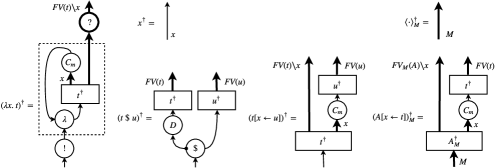
Figure 5: Inductive Translation of Terms and Answer Contexts

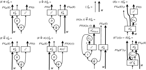
Figure 6: Inductive Translation of Evaluation Contexts

The two mutually recursive translations $(\cdot)^{\dagger}$ and $(\cdot)^{\ddagger}$ are related by the following decompositions, which can be checked by straightforward induction. In the third decomposition, $M^{\prime}$ is not captured in $E$.

Note that the decomposition property like the fourth one does not hold for $E\langle t\rangle$ in general, because a translation $(A\langle\lambda{x}.t\rangle\mathbin{\overrightarrow{@}}E)^{\ddagger}_{\_}M$ lacks a $\mathop{!}$-box structure, compared to a translation $(A\langle\lambda{x}.t\rangle\mathbin{\overrightarrow{@}}u)^{\dagger}$.

The inductive translations lift to a binary relation between closed enriched terms and graph states.

Definition 4.2 (Binary relation $\preceq$).

The binary relation $\preceq$ is defined by $E\langle\llparenthesis t\rrparenthesis\rangle\preceq((E^{\ddagger}\circ t^{\dagger},e),(\mathord{\uparrow},\square,S,B))$, where: (i) $E\langle\llparenthesis t\rrparenthesis\rangle$ is a closed enriched term, and $(E^{\ddagger}\circ t^{\dagger},e)$ is given by with no edges between links, and (ii) there is an execution $\mathit{Init}(E^{\ddagger}\circ t^{\dagger})\to^{*}((E^{\ddagger}\circ t^{\dagger},e),(\mathord{\uparrow},\square,S,B))$ such that the position $e$ appears only in the last state of the sequence.

A special case is $\llparenthesis t\rrparenthesis\preceq\mathit{Init}(t^{\dagger})$, which relates the starting points of an evaluation and an execution. We require the graph $E^{\ddagger}\circ t^{\dagger}$ to have no edges between links, which is based on the discussion at the end of Sec. 3 and essential for time-cost analysis. Although the definition of the translations relies on edges between links (e.g. the translation $x^{\dagger}$), we can safely replace any consecutive links in the composition of translations $E^{\ddagger}$ and $t^{\dagger}$ with a single link, and yield the graph $E^{\ddagger}\circ t^{\dagger}$ with no consecutive links.

The binary relation $\preceq$ gives a weak simulation of the sub-machine semantics by the graph-rewriting machine. The weakness, i.e. the extra transitions compared with reductions, comes from the locality of pass transitions and the bureaucracy of managing $\mathop{!}$-boxes.

Theorem 4.3 (Weak simulation with global bound).

1. If $E\langle\llparenthesis t\rrparenthesis\rangle\multimap_{\_}\chi E^{\prime}\langle\llparenthesis t^{\prime}\rrparenthesis\rangle$ and $E\langle\llparenthesis t\rrparenthesis\rangle\preceq((E^{\ddagger}\circ t^{\dagger},e),\delta)$ hold, then there exists a number $n\leq 3$ and a graph state $(((E^{\prime})^{\ddagger}\circ(t^{\prime})^{\dagger},e^{\prime}),\delta^{\prime})$ such that $((E^{\ddagger}\circ t^{\dagger},e),\delta)\to_{\_}\epsilon^{n}\to_{\_}\chi(((E^{\prime})^{\ddagger}\circ(t^{\prime})^{\dagger},e^{\prime}),\delta^{\prime})$ and $E^{\prime}\langle\llparenthesis t^{\prime}\rrparenthesis\rangle\preceq(((E^{\prime})^{\ddagger}\circ(t^{\prime})^{\dagger},e^{\prime}),\delta^{\prime})$.

2. If $A\langle\llparenthesis v\rrparenthesis\rangle\preceq((A^{\ddagger}\circ v^{\dagger},e),\delta)$ holds, then the graph state $((A^{\ddagger}\circ v^{\dagger},e),\delta)$ is initial, from which only the transition $\mathit{Init}(A^{\ddagger}\circ v^{\dagger})\to_{\_}\epsilon\mathit{Final}(A^{\ddagger}\circ v^{\dagger})$ is possible.

Proof outline.

The second half of the theorem is straightforward. For the first half, Fig. 7 and Fig. 8 illustrate how the graph-rewriting machine simulates each reduction $\multimap$ of the sub-machine semantics. Annotations of edges are omitted. The figures altogether include ten sequences of translations $\to$, whose only first and last graph states are shown. Each sequence simulates a single reduction $\multimap$, and is preceded by a number (i.e. (1)) that corresponds to a basic rule applied by the reduction (see Fig. 1). Some sequences involve equations that apply the four decomposition properties of the translations $(\cdot)^{\dagger}$ and $(\cdot)^{\ddagger}$, which are given earlier in this section. These equations rely on the fact that reductions with labels $\beta$ and $\sigma$ work modulo alpha-equivalence to avoid name captures. This means that (i) free variables of $u$ (resp. $A^{\prime}\langle v\rangle$) are never captured by $A$ in the reduction (2) (resp. (5) and (8)), (ii) the variable $x$ is never captured by $E$ or $E^{\prime}$, and (iii) free variables of $E$ are never captured by $A$. Especially in simulation of the reduction (9), the variable $x$ is not captured by the evaluation context $E^{\prime}$, and therefore the first token position is in fact an input of the $\mathit{C}_{\_}{m+1}$-node. ∎

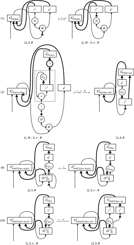
Figure 7: Illustration of Simulation: Call-by-Need Application and Explicit Substitutions

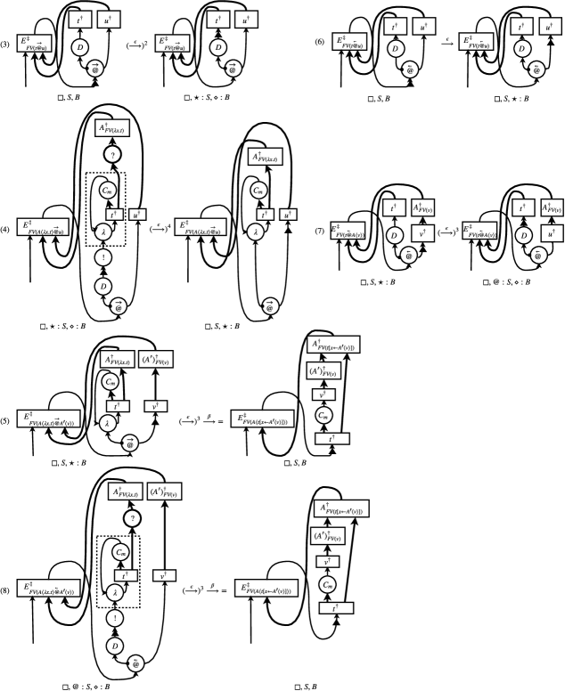
Figure 8: Illustration of Simulation: Left-to-Right and Right-to-Left Call-by-Value Applications

We analyse how time-efficiently the token-guided graph-rewriting machine implements evaluation strategies, following the methodology developed by Accattoli et al. [3, 7, 2]. The methodology tracks the number of beta-reduction steps in an evaluation in three steps: (I) bound the number of transitions required in implementing evaluation strategies, (II) estimate time cost of each transition, and (III) bound overall time cost of implementing evaluation strategies, by multiplying the number of transitions with time cost for each transition.

Given a pure term $t$, the time cost of an execution on the graph $t^{\dagger}$ is estimated by means of: (i) the number of reductions labelled with $\beta$ in the evaluation of the term $t$, and (ii) the size $|t|$ of the term $t$, inductively defined as: $|x|:=1$, $|\lambda{x}.t|:=|t|+1$, $|t\mathbin{@}u|=|t\mathbin{\overrightarrow{@}}u|=|t\mathbin{\overleftarrow{@}}u|:=|t|+|u|+1$, $|t[x\leftarrow u]|:=|t|+|u|+1$.

Given an evaluation $\mathit{Eval}$, the number of occurrences of a label $\chi$ is denoted by $|\mathit{Eval}|_{\_}\chi$. The sub-machine semantics comes with the following quantitative bounds.

Proposition 4.4.

For any evaluation $\mathit{Eval}\colon\llparenthesis t\rrparenthesis\to^{*}A\langle\llparenthesis v\rrparenthesis\rangle$ that terminates, the number of reductions is bounded by $|\mathit{Eval}|_{\_}\sigma=\mathcal{O}(|\mathit{Eval}|_{\_}\beta)$ and $|\mathit{Eval}|_{\_}\epsilon=\mathcal{O}(|t|\cdot|\mathit{Eval}|_{\_}\beta).$

Proof outline.

A term uses a single evaluation strategy, either call-by-need, left-to-right call-by-value, or right-to-left call-by-value. The proof is by developing the one-to-one correspondence between an evaluation by the sub-machine semantics and a “derivation” in the linear substitution calculus. This goes in the same way Accattoli et al. analyse various abstract machines [3], especially the proof of the second equation [3, Thm. 11.3 & Thm. 11.5]. The first equation is a direct application of the bounds about the linear substitution calculus [7, Cor. 1 & Thm. 2]. ∎

We use the same notation $|\mathit{Exec}|_{\_}\chi$, as for an evaluation, to denote the number of occurrences of each label $\chi$ in an execution $\mathit{Exec}$. Additionally the number of rewrite transitions with the label $\epsilon$ is denoted by $|\mathit{Exec}|_{\_}\mathit{\epsilon R}$. The following proposition completes the first step of the cost analysis.

Proposition 4.5 (Soundness & completeness, with number bounds).

For any pure closed term $t$, an evaluation $\mathit{Eval}\colon\llparenthesis t\rrparenthesis\to^{*}A\langle\llparenthesis v\rrparenthesis\rangle$ terminates with the enriched term $A\langle\llparenthesis v\rrparenthesis\rangle$ if and only if an execution $\mathit{Exec}\colon\mathit{Init}(t^{\dagger})\to^{*}\mathit{Final}(A^{\ddagger}\circ v^{\dagger})$ terminates with the graph $A^{\ddagger}\circ v^{\dagger}$. Moreover the number of transitions is bounded by $|\mathit{Exec}|_{\_}\beta=|\mathit{Eval}|_{\_}\beta$, $|\mathit{Exec}|_{\_}\sigma=\mathcal{O}(|\mathit{Eval}|_{\_}\beta)$, $|\mathit{Exec}|_{\_}\epsilon=\mathcal{O}(|t|\cdot|\mathit{Eval}|_{\_}\beta)$, $|\mathit{Exec}|_{\_}\mathit{\epsilon R}=\mathcal{O}(|\mathit{Eval}|_{\_}\beta)$.

Proof.

This proposition is a direct consequence of Thm. 4.3 and Prop. 4.4, except for the last bound. The last bound of $|\mathit{Exec}|_{\_}\mathit{\epsilon R}$ follows from the fact that each rewrite transition labelled with $\beta$ is always preceded by one rewrite transition labelled with $\epsilon$. ∎

The next step in the cost analysis is to estimate the time cost of each transition. We assume that graphs are implemented in the following way. Each link is given by two pointers to its child and its parent, and each node is given by its label and pointers to its outputs. Abstraction nodes ($\lambda$) and application nodes ($\mathbin{@}$, $\mathbin{\overrightarrow{@}}$ and $\mathbin{\overleftarrow{@}}$) have two pointers that are distinguished, and all the other nodes have only one pointer to their unique output. Additionally each $\mathop{!}$-node has pointers to inputs of its associated $\wn$-nodes, to represent a $\mathop{!}$-box structure. Accordingly, a position of the token is a pointer to a link, a direction and a rewrite flag are two symbols, a computation stack is a stack of symbols, and finally a box stack is a stack of symbols and pointers to links.

Using these assumptions of implementation, we estimate time cost of each transition. All pass transitions have constant cost. Each pass transition looks up one node and its outputs (that are either one or two) next to the current position, and involves a fixed number of elements of the token data. Rewrite transitions with the label $\beta$ have constant cost, as they change a constant number of nodes and links, and only a rewrite flag of the token data. Rewrite transitions with the label $\epsilon$ remove a $\mathop{!}$-box structure, and hence have cost bounded by the number of the auxiliary doors. Finally, rewrite transitions with the label $\sigma$ copy a $\mathop{!}$-box structure. Copying cost is bounded by the size of the $\mathop{!}$-box, i.e. the number of nodes and links in the $\mathop{!}$-box. Updating cost of the sub-graph $H^{\prime}$ (see Fig. 4) is bounded by the number of auxiliary doors, that is less than the size of the copied $\mathop{!}$-box. The assumption about the implementation of graphs enables us to conclude updating cost of the $\mathit{C}$-node is constant.

With the results of the previous two steps, we can now give the overall time cost of executions.

Theorem 4.6 (Soundness & completeness, with cost bounds).

For any pure closed term $t$, an evaluation $\mathit{Eval}\colon\llparenthesis t\rrparenthesis\to^{*}A\langle\llparenthesis v\rrparenthesis\rangle$ terminates with the enriched term $A\langle\llparenthesis v\rrparenthesis\rangle$ if and only if an execution $\mathit{Exec}\colon\mathit{Init}(t^{\dagger})\to^{*}\mathit{Final}(A^{\ddagger}\circ v^{\dagger})$ terminates with the graph $A^{\ddagger}\circ v^{\dagger}$. The overall time cost of the execution $\mathit{Exec}$ is bounded by $\mathcal{O}(|t|\cdot|\mathit{Eval}|_{\_}\beta)$.

Proof.

Non-constant cost of rewrite transitions are either the number of auxiliary doors of a $\mathop{!}$-box or the size of a $\mathop{!}$-box. The former can be bounded by the latter, which is no more than the size of the initial graph $t^{\dagger}$, by Lem. 3.2. The size of the initial graph $t^{\dagger}$ can be bounded by the size $|t|$ of the initial term. Therefore any non-constant cost of each rewrite transition, in the execution $\mathit{Exec}$, can be also bounded by $|t|$. The overall time cost of rewrite transitions labelled with $\beta$ is $\mathcal{O}(|\mathit{Eval}|_{\_}\beta)$, and that of the other rewrite transitions and pass transitions is $\mathcal{O}(|t|\cdot|\mathit{Eval}|_{\_}\beta)$. ∎

Thm. 4.6 classifies the graph-rewriting machine as “efficient,” by Accattoli’s taxonomy [2, Def. 7.1] of abstract machines. The efficiency benefits from the graphical representation of environments (i.e. explicit substitutions in our setting). In particular the translations $(\cdot)^{\dagger}$ and $(\cdot)^{\ddagger}$ are carefully designed to exclude any two sequentially-connected $\mathit{C}$-nodes, which yields the constant cost to look up a bound variable and its associated computation in environments.

5 Related Work and Conclusions

In an abstract machine of any functional programming language, computations assigned to variables have to be stored for later use. Potentially multiple, conflicting, computations can be assigned to a single variable, primarily because of multiple uses of a function with different arguments. Different solutions to this conflict lead to different representations of the storage, some of which are examined by Accattoli and Barras [4] from the perspective of time-cost analysis. We recall a few solutions below that seem relevant to our token-guided graph-rewriting.

One solution is to allow at most one assignment to each variable. This is typically achieved by renaming bound variables during execution, possibly symbolically. Examples for call-by-need evaluation are Sestoft’s abstract machines [26], and the storeless and store-based abstract machines studied by Danvy and Zerny [11]. Our graph-rewriting abstract machine gives another example, as shown by the simulation of the sub-machine semantics that resembles the storeless abstract machine mentioned above. Variable renaming is trivial in our machine, thanks to the use of graphs in which variables are represented by mere edges.

Another solution is to allow multiple assignments to a variable, with restricted visibility. The common approach is to pair a sub-term with its own “environment” that maps its free variables to their assigned computations, forming a so-called “closure.” Conflicting assignments are distributed to distinct localised environments. Examples include Cregut’s lazy variant [8] of Krivine’s abstract machine for call-by-need evaluation, and Landin’s SECD machine [19] for call-by-value evaluation. Fernández and Siafakas [14] refine this approach for call-by-name and call-by-value evaluations, based on closed reduction [13], which restricts beta-reduction to closed function arguments. This suggests that the approach with localised environments can be modelled in our setting by implementing closed reduction. The implementation would require an extension of rewrite transitions and a different strategy to trigger them, namely to eliminate auxiliary doors of a $\mathop{!}$-box.

Additionally, Fernández and Siafakas [14] propose another approach to multiple assignments, in which multiple assignments are augmented with binary strings so that each occurrence of a variable can only refer to one of them. This approach is based on a GoI-style token-passing abstract machine for call-by-value evaluation, designed by Fernández and Mackie [12]. The machine keeps the underlying graph fixed during execution and allows the token to jump along a path in the graph. It therefore recovers time efficiency, although no quantitative analysis is provided. Jumps can be seen as a form of graph rewriting that eliminates nodes. Some jumps are to or from edges with an index that are effectively “virtual” copies of edges.

To wrap up, we presented a graph-rewriting abstract machine, with token passing as a guide, that can time-efficiently implement three evaluation strategies that have different control over caching intermediate results. The idea of using the token as a guide of graph rewriting was also proposed by Sinot [27, 28] for interaction nets. He shows how using a token can make the rewriting system implement the call-by-name, call-by-need and call-by-value evaluation strategies. Our development in this work can be seen as a realisation of the rewriting system as an abstract machine, in particular with explicit control over copying sub-graphs. The GoI-style token passing itself has been adapted to implement the call-by-value evaluation strategy. Apart from the abstract machine with jumps [12] already mentioned, known adaptations [25, 17] commonly use the CPS transformation [24], with the focus on correctness. However this method naively leads to an abstract machine with inefficient overhead cost [17].

The token-guided graph rewriting is a flexible framework in which we can carry out the study of space-time trade-off in abstract machines for various evaluation strategies of the lambda-calculus. Starting with the previous work [23] and continuing with the present work, our focus was primarily on time-efficiency. This is to complement existing work on GoI-style operational semantics which usually achieves space-efficiency, and also to confirm that introduction of graph rewriting to the semantics does not bring in any hidden inefficiencies. We believe that more refined strategies of interleaving token routing and graph reduction can be formulated to serve particular objectives in the space-time execution efficiency trade-off.

Acknowledgement

We thank Steven Cheung for helping us implement the on-line visualiser.

References

- [1]
- [2] Beniamino Accattoli (2017): The complexity of abstract machines. In: WPTE 2016, EPTCS 235, pp. 1–15, 10.4204/EPTCS.235.1.
- [3] Beniamino Accattoli, Pablo Barenbaum & Damiano Mazza (2014): Distilling abstract machines. In: ICFP 2014, ACM, pp. 363–376, 10.1145/2628136.2628154.
- [4] Beniamino Accattoli & Bruno Barras (2017): Environments and the complexity of abstract machines. In: PPDP 2017, ACM, pp. 4–16, 10.1145/3131851.3131855.
- [5] Beniamino Accattoli & Ugo Dal Lago (2016): (Leftmost-outermost) beta reduction is invariant, indeed. Logical Methods in Comp. Sci. 12(1), 10.2168/LMCS-12(1:4)2016.
- [6] Beniamino Accattoli & Stefano Guerrini (2009): Jumping boxes. In: CSL 2009, Lect. Notes Comp. Sci. 5771, Springer, pp. 55–70, 10.1007/978-3-642-04027-67.
- [7] Beniamino Accattoli & Claudio Sacerdoti Coen (2014): On the value of variables. In: WoLLIC 2014, Lect. Notes Comp. Sci. 8652, Springer, pp. 36–50, 10.1007/978-3-662-44145-93.
- [8] Pierre Crégut (2007): Strongly reducing variants of the Krivine abstract machine. Higher-Order and Symbolic Computation 20(3), pp. 209–230, 10.1007/s10990-007-9015-z.
- [9] Vincent Danos & Laurent Regnier (1996): Reversible, irreversible and optimal lambda-machines. Elect. Notes in Theor. Comp. Sci. 3, pp. 40–60, 10.1016/S1571-0661(05)80402-5.
- [10] Olivier Danvy, Kevin Millikin, Johan Munk & Ian Zerny (2012): On inter-deriving small-step and big-step semantics: a case study for storeless call-by-need evaluation. Theor. Comp. Sci. 435, pp. 21–42, 10.1016/j.tcs.2012.02.023.
- [11] Olivier Danvy & Ian Zerny (2013): A synthetic operational account of call-by-need evaluation. In: PPDP 2013, ACM, pp. 97–108, 10.1145/2505879.2505898.
- [12] Maribel Fernández & Ian Mackie (2002): Call-by-value lambda-graph rewriting without rewriting. In: ICGT 2002, LNCS 2505, Springer, pp. 75–89, 10.1007/3-540-45832-88.
- [13] Maribel Fernández, Ian Mackie & François-Régis Sinot (2005): Closed reduction: explicit substitutions without alpha-conversion. Math. Struct. in Comp. Sci. 15(2), pp. 343–381, 10.1017/S0960129504004633.
- [14] Maribel Fernández & Nikolaos Siafakas (2009): New developments in environment machines. Elect. Notes in Theor. Comp. Sci. 237, pp. 57–73, 10.1016/j.entcs.2009.03.035.
- [15] Jean-Yves Girard (1987): Linear logic. Theor. Comp. Sci. 50, pp. 1–102, 10.1016/0304-3975(87)90045-4.
- [16] Jean-Yves Girard (1989): Geometry of Interaction I: interpretation of system F. In: Logic Colloquium 1988, Studies in Logic & Found. Math. 127, Elsevier, pp. 221–260, 10.1016/S0049-237X(08)70271-4.
- [17] Naohiko Hoshino, Koko Muroya & Ichiro Hasuo (2014): Memoryful Geometry of Interaction: from coalgebraic components to algebraic effects. In: CSL-LICS 2014, ACM, pp. 52:1–52:10, 10.1145/2603088.2603124.
- [18] Aleks Kissinger (2012): Pictures of processes: automated graph rewriting for monoidal categories and applications to quantum computing. CoRR abs/1203.0202. Available at http://arxiv.org/abs/1203.0202.
- [19] Peter Landin (1964): The mechanical evaluation of expressions. The Comp. Journ. 6(4), pp. 308–320, 10.1093/comjnl/6.4.308.
- [20] Ian Mackie (1995): The Geometry of Interaction machine. In: POPL 1995, ACM, pp. 198–208, 10.1145/199448.199483.
- [21] John Maraist, Martin Odersky, David N. Turner & Philip Wadler (1999): Call-by-name, call-by-value, call-by-need and the linear lambda calculus. Theor. Comp. Sci. 228(1-2), pp. 175–210, 10.1016/S0304-3975(98)00358-2.
- [22] Paul-André Melliès (2006): Functorial boxes in string diagrams. In: CSL 2006, Lect. Notes Comp. Sci. 4207, Springer, pp. 1–30, 10.1007/118746831.
- [23] Koko Muroya & Dan R. Ghica (2017): The dynamic Geometry of Interaction machine: a call-by-need graph rewriter. In: CSL 2017, LIPIcs 82, pp. 32:1–32:15, 10.4230/LIPIcs.CSL.2017.32.
- [24] Gordon Plotkin (1975): Call-by-name, call-by-value and the lambda-calculus. Theor. Comp. Sci. 1(2), pp. 125–259, 10.1016/0304-3975(75)90017-1.
- [25] Ulrich Schöpp (2014): Call-by-value in a basic logic for interaction. In: APLAS 2014, Lect. Notes Comp. Sci. 8858, Springer, pp. 428–448, 10.1007/978-3-319-12736-123.
- [26] Peter Sestoft (1997): Deriving a lazy abstract machine. J. Funct. Program. 7(3), pp. 231–264, 10.1017/S0956796897002712.
- [27] François-Régis Sinot (2005): Call-by-name and call-by-value as token-passing interaction nets. In: TLCA 2005, Lect. Notes Comp. Sci. 3461, Springer, pp. 386–400, 10.1007/1141717028.
- [28] François-Régis Sinot (2006): Call-by-need in token-passing nets. Math. Struct. in Comp. Sci. 16(4), pp. 639–666, 10.1017/S0960129506005408.