Examples of tropical-to-Lagrangian correspondence

Abstract.

The paper associates Lagrangian submanifolds in symplectic toric varieties to certain tropical curves inside the convex polyhedral domains of $\mathbb{R}^{n}$ that appear as the images of the moment map of the toric varieties.

We pay a particular attention to the case $n=2$, where we reprove Givental’s theorem [6] on Lagrangian embeddability of non-oriented surfaces to $\mathbb{C}^{2}$, as well as to the case $n=3$, where we see appearance of the graph 3-manifolds studied by Waldhausen [24] as Lagrangian submanifolds. In particular, rational tropical curves in $\mathbb{R}^{3}$ produce 3-dimensional rational homology spheres. The order of their first homology groups is determined by the multiplicity of tropical curves in the corresponding enumerative problems.

1. Some background material

1.1. Symplectic toric varieties and the moment map.

Let $\Lambda\approx\mathbb{Z}^{n}$ be a free Abelian group (a lattice) of rank $n$. Let $A\approx\mathbb{R}^{n}$ be an affine space over the real $n$-dimensional vector space $\Lambda\otimes\mathbb{R}$. Clearly we can identify $T_{x}A=\Lambda\otimes\mathbb{R}$ for the tangent space to $A$ at any $x\in A$. In particular, the tangent spaces at all points of $A$ are canonically identified.

Furthermore, as $A$ is an affine space over $T_{x}A$ a choice of $x$ gives an identification between $A$ and $\Lambda\otimes\mathbb{R}$, $A\ni y\mapsto y-x\in\Lambda\otimes\mathbb{R}$. Thus an element $p$ of the dual lattice $\Lambda^{*}=\operatorname{Hom}(\Lambda,\mathbb{Z})$ and a point $x\in A$ define an affine function $p^{x}:A\to\mathbb{R}$ by $y\mapsto\ <p,y-x>$.

We refer to $A$ as the tropical affine space (more classically it is an affine space corresponding to the structure group obtained from the integer linear group $GL(n,\mathbb{Z})$ by extending it with all real translations in $\mathbb{R}^{n}$).

Definition 1.1.

A polyhedral domain $\Delta\subset A$ is the intersection of a finite number of half-spaces $\{x\in A\ |\ p^{y}_{j}x\geq a_{j}\}$, $j=1,\dots,N$, $y\in A$, $a_{j}\in\mathbb{R}$ and $p_{j}\in\Lambda^{*}$ such that the interior of $\Delta$ is non-empty.

A point $z\in\Delta$ is called smooth if there exists an open neighborhood $U\ni z$, a point $y\in\mathbb{R}^{n}$ and an integer basis $\{p_{1},\dots,p_{n}\}\subset\Lambda^{*}$ such that

$$U\cap\Delta=\bigcap\limits_{j=1}^{n}\{x\in\mathbb{R}^{n}\ |\ p^{y}_{j}x\geq 0\}.$$

A polyhedral domain is called Delzant, if all its points are smooth.

Suppose that $(M,\omega)$ is a $2n$-dimensional symplectic manifold with a Hamiltonian action of the real $n$-torus $T=(S^{1})^{n}$, and $\mu:M\to t^{*}$ is the corresponding moment map, defined by

(1) $$<Y,d\mu(X)>\ =2\pi\omega(X,Y),$$

for any $Y\in t$, $X\in T_{u}M$, $u\in M$. Here $t^{*}$ is the dual vector space to the Lie algebra $t$ of $T$. The element $Y\in t$ yields a vector field on $M$ through the action of $T$ on $M$, thus the left-hand side of (1) is well-defined for any $X\in T_{u}M$. The condition (1) defines $\mu$ up to a translation in $t^{*}$, see e.g. [1] for details.

Note that the Lie algebra $t$ comes with a natural lattice $\Lambda^{*}\approx\mathbb{Z}^{n}$ defined as $\exp^{-1}(0)$ for the exponent map $\exp:t\to T$ so that $T=t/\Lambda^{*}$. We have $t^{*}=\Lambda\otimes\mathbb{R}$ for $\Lambda=\operatorname{Hom}(\Lambda^{*},\mathbb{Z})$. Since $\mu$ is defined up to a translation, its target has a natural structure of an affine space over $A$, i.e. the tropical affine space. We write

(2) $$\mu:M\to A$$

for the moment map of $(M,\omega)$. The fibers of the moment map coincide with the orbits of the action of $T$.

Definition 1.2.

A symplectic toric variety is a $2n$-dimensional symplectic manifold $(M,\omega)$ with a Hamiltonian action of the real $n$-torus $T$ such that $\mu(M)$ is a polyhedral domain.

Remark 1.3.

If $(M,\omega)$ is compact $2n$-dimensional symplectic manifold with a Hamiltonian action of the real $n$-torus $T$ then $\mu(M)$ is automatically a polyhedral domain, and furthermore is always smooth. For non-compact $M$ then the condition that $\mu(M)$ is polyhedral is a certain completeness condition on $\omega$.

For any Delzant polyhedral domain $\Delta\subset A$ there exists a symplectic toric variety $(M_{\Delta},\omega_{\Delta})$ with $\mu(M_{\Delta})=\Delta$, see [5].

Example 1.4.

Suppose $\Delta=A$. The cotangent space $T^{*}A$ has a canonical symplectic structure $\omega=d\alpha$, $\alpha=pdq$, $q\in A$, $p\in T_{q}A$ (so that $\alpha$ is a well-defined non-closed 1-form). The Lie algebra $t=\Lambda^{*}\otimes\mathbb{R}$ acts on $T^{*}A$ by translations preserving the form $\omega$. Thus the quotient space $M=(T^{*}A)/\Lambda^{*}$ together with the form $\omega$ is a symplectic manifold with an action of $T=t/\Lambda^{*}$. According to (1) the moment map is given by the projection onto $A$,

$$\mu:M\to A,\ (p,q)\mapsto q.$$

The quotient $(M,\omega)$ may be identified with the complex $n$-torus $(\mathbb{C}^{\times})^{n}$ enhanced with a $(\mathbb{C}^{\times})^{n}$-invariant symplectic form

$$\omega_{(\mathbb{C}^{\times})^{n}}=\frac{i}{2}\sum\limits_{j=1}^{n}\frac{dz_{j}}{z_{j}}\wedge\frac{d\bar{z}_{j}}{\bar{z}_{j}}.$$

The torus $T=(S^{1})^{n}$ acts on $(\mathbb{C}^{\times})^{n}$ by coordinatewise multiplication (we identify $S^{1}$ with a unit circle in $\mathbb{C}$). The moment map $\mu:(\mathbb{C}^{\times})^{n}\to A$ coincides with $\operatorname{Log}:(\mathbb{C}^{\times})^{n}\to\mathbb{R}^{n}$,

$$\operatorname{Log}(z_{1},\dots,z_{n})=(\log|z_{1}|,\dots,\log|z_{n}|)$$

after the identification of $A$ with $\mathbb{R}^{2}$. In other words, we have a symplectomorphism between $((\mathbb{C}^{\times})^{n},\omega_{(\mathbb{C}^{\times})^{n}})$ and $(M,\omega=\sum\limits_{j=1}^{n}dp_{j}\wedge dq_{j})$ given by

$$q_{j}=\log|z_{j}|,\ p_{j}=\arg(z_{j}).$$

If $\Delta\neq A$ then for each (open) face $E\subset\partial\Delta$ of codimension $k$ the inverse image $\mu^{-1}(E)$ is fibered by $k$-dimensional tori whose tangent vectors are contained in the radical of the form $\omega$ restricted to the tangent space of $\mu^{-1}(E)$. Taking the quotient of $\mu^{-1}(\Delta)$ by this fibration over all the faces of $\partial\Delta$ is known as the symplectic reduction. In the case when $\Delta$ is a Delzant polyhedral domain, this construction produces a smooth $2n$-dimensional symplectic manifold $(M_{\Delta}=\mu^{-1}(\Delta)/\sim,\omega_{\Delta})$ with a Hamiltonian action of $T$ such that the moment map $\mu$ descends by the projection $\mu^{-1}(\Delta)\to M_{\Delta}$ to the moment map $\mu_{\Delta}:M_{\delta}\to A$, and the symplectic forms $\omega_{\Delta}$ and $\omega$ agree on $M_{\Delta}\smallsetminus\mu^{-1}(\partial\Delta)\subset M$. In particular, we have $\mu_{\Delta}(M_{\Delta})=\Delta$.

1.2. Tropical curves in $\Delta$

Let $\bar{\Gamma}$ be a topological space homeomorphic to a finite graph. The subset $\partial\Gamma\subset\bar{\Gamma}$ of 1-valent vertices and the subset $V_{\Gamma}$ of vertices of valence greater than 2 do not depend on the choice of a graph model for $\bar{\Gamma}$, and thus are well-defined subspaces in the topological space $\bar{\Gamma}$.

We set $\Gamma=\bar{\Gamma}\smallsetminus\partial\Gamma$. Connected components of $\Gamma\smallsetminus V_{\Gamma}$ are homeomorphic to open intervals and are called edges of $\Gamma$. The set of edges of $\Gamma$ is denoted with $E_{\Gamma}$. An edge is called a leaf if it is adjacent to $\partial\Gamma$ and and a bounded edge otherwise.

Definition 1.5.

The topological space $\Gamma$ enhanced with an inner complete metric is called a (smooth, irreducible and explicit) tropical curve.

Specifying an inner metric on $\Gamma$ amounts to specifying positive lengths of the edges of the graph. By the completeness assumption the lengths of the leaves must be infinite while the lengths of the bounded edges are finite.

Remark 1.6.

Definition 1.5 introduces smooth, irreducible and explicit tropical curves. For the purposes of this paper we refer to such curves simply as tropical curves. In a more general framework, there is a genus function (cf. e.g. [3]) $V_{\Gamma}\to\mathbb{Z}_{\geq 0}$ which can also be reformulated as a $\chi$-measure (cf. e.g. [7]). Then the set $V_{\Gamma}$ also includes vertices of valence 1 or 2 with positive values of the genus function. Such generalized curves are needed for compactifications of moduli spaces of tropical curves. In this paper we do not use them. Our tropical curves have the genus function equal to zero everywhere on $V_{\Gamma}$.

Recall that a continuous map $f:X\to Y$ between topological spaces is called an immersion if it is a local embedding, i.e. for any $x\in X$ there exists an open neighborhood $U\ni x$ such that $f|_{U}$ is an embedding of $U$ to $Y$.

Definition 1.7.

An immersion $h:\Gamma\to A$ (between topological spaces $\Gamma$ and $A$) is called tropical [14], if the following conditions hold.

• For any edge $e\in E_{\Gamma}$, a point $x\in e$ and a unit tangent vector $u\in T_{x}e$ the restriction $h|_{e}$ is a smooth map such that

  $$dh_{x}(u)\in\Lambda\subset T_{h(x)}A.$$

  In particular, $dh_{x}(u)$ does not depend on the choice of $x\in e$ and depends only on the orientation of $e$ given by $u$. We denote $dh(e)=dh_{x}(u)\in\Lambda$ for the oriented edge $e$.

• For any vertex $v\in V_{\Gamma}$ we have

  $$\sum\limits_{\bar{e}\ni v}dh(e)=0,$$

  where the sum is taken over all edges $e$ adjacent to $v$. The orientation of $e$ is chosen to be away from $v$. This condition is known as the balancing condition.

The tropical immersion is called locally flat if, in addition, the following condition holds.

• If a collection of edges $\{e_{j}\}\subset E_{\Gamma}$ is adjacent to the same vertex $v\in V_{\Gamma}$ then the linear span of $\{dh(e_{j})\}$ in $\Lambda\otimes\mathbb{R}$ is 2-dimensional.

The intersection $h(\Gamma)\cap\Delta\subset\Delta$ is called a locally flat tropical curve in a polyhedral domain $\Delta$.

Note that if $\Gamma$ is 3-valent then any tropical immersion $h:\Gamma\to A$ is locally flat as a consequence of the balancing condition.

Definition 1.8.

A tropical immersion $h:\Gamma\to A$ is called primitive if the following conditions hold.

• The tropical curve $\Gamma$ is connected, 3-valent, and $V_{\Gamma}\neq\emptyset$.

• For any $e\in E_{\Gamma}$ the vector $dh(e)$ is primitive element of the lattice $\Lambda$.

• If $x\neq y\in\Gamma$ and $h(x)=h(y)$ then $x,y\in\Gamma\smallsetminus V_{\Gamma}$.

The image $h(\Gamma)$ is called a primitive tropical curve in $A$.

Definition 1.9.

Let $\Delta\subset A$ be a polyhedral domain and $\Gamma_{\Delta}$ be a topological space homeomorphic to a connected graph. An immersion $h_{\Delta}:\Gamma_{\Delta}\to\Delta$ is called $\Delta$-tropical (or just tropical) if there exists a tropical immersion $h:\Gamma\to A$ such that $\Gamma_{\Delta}\subset\Gamma$, $h|_{\Gamma_{\Delta}}=h_{\Delta}$ and $h^{-1}(\partial\Delta)$ is a finite set disjoint from $V_{\Gamma}$. A $\Delta$-tropical immersion $h_{\Delta}$ is called primitive if $h$ can be chosen to be primitive and $\#(h^{-1}(x))=1$ whenever $x\in\partial\Delta$. The symbol $\#$ stands for the cardinality of a set.

A subset $C\subset\Delta$ is called a primitive tropical curve in $\Delta$ if there exists a primitive $\Delta$-tropical immersion $h_{\Delta}:\Gamma_{\Delta}\to\Delta$ such that $h_{\Delta}(\Gamma_{\Delta})=C$.

Proposition 1.10.

If $C\subset\Delta$ is a primitive tropical curve in $\Delta$ then a primitive $\Delta$-tropical immersion with $C=h_{\Delta}(\Gamma_{\Delta})\cap\Delta$ is unique. Furthermore, the self-intersection set

(3) $$\Sigma(C)=\{z\in C\ |\ \#(h_{\Delta}^{-1}(z))>1\}$$

of $h_{\Delta}$ is finite.

Proof.

Suppose that $h_{\Delta}:\Gamma_{\Delta}\to\Delta$, $h^{\prime}_{\Delta}:\Gamma^{\prime}_{\Delta}\to\Delta$ are two primitive $\Delta$-tropical immersions and $h:\Gamma\to A$, $h^{\prime}:\Gamma^{\prime}\to A$ be tropical immersions with $h_{\Delta}=h|_{\Gamma_{\Delta}}$ and $h^{\prime}_{\Delta}=h^{\prime}|_{\Gamma^{\prime}_{\Delta}}$. Let $v\in V_{\Gamma}\cap\Gamma_{\Delta}$. By the conditions $(i)$ and $(ii)$ of Definition 1.8, and since $h$ is a topological immersion, a small neighborhood of $v$ in $\Gamma_{\Delta}$ and that of $h(v)$ in $C$ are homeomorphic. Thus $h(v)=h^{\prime}(v^{\prime})$ for $v^{\prime}\in V_{\Gamma^{\prime}}\cap\Gamma^{\prime}_{\Delta}$. By the condition $(iii)$, we get a 1-1 correspondence between $V_{\Gamma}\cap\Gamma_{\Delta}$ and $V_{\Gamma^{\prime}}\cap\Gamma^{\prime}_{\Delta}$. Similarly, we get a 1-1 correspondence between $h^{-1}(\partial\Delta)$ and $h^{\prime-1}(\partial\Delta)$. Also by $(iii)$ if $e_{1},e_{2}\in E_{\Gamma}$ are such that $h(e_{1})\neq h(e_{2})$ then $h(e_{1})$ is transversal to $h(e_{2})$. This implies that the obtained correspondences extend to a homeomorphism $\Phi:\Gamma_{\Delta}\to\Gamma^{\prime}_{\Delta}$ such that $h^{\prime}_{\Delta}=h_{\Delta}\circ\Phi$. The same property implies the finiteness of $\Sigma$. ∎

Thus we may speak of the vertices $V_{C}=h_{\Delta}(\Gamma_{\Delta})$ of $C$.

The boundary points of a primitive tropical curve $C$ in $\Delta$ are the points of its (topological) boundary $\partial C=C\cap\partial\Delta$. Each boundary point belongs to a unique $(n-k)$-dimensional (relatively open) face of the polyhedral domain $\Delta$. We call $k$ the codimension of a boundary point $x\in\partial C$.

Definition 1.11.

Let $x\in\partial C$ be a boundary point of codimension 1, $e_{x}\in E_{\Gamma}$ be the edge containing $h^{-1}(x)$, and $\Delta_{x}\subset\partial\Delta$ be the facet containing $x$. The boundary momentum $p(x)\in\mathbb{N}$ is the tropical intersection number of $h(e_{x})$ and $\Delta_{x}$ in $A$, i.e. the index in $\Lambda$ of the sublattice generated by $dh(e_{x})$ and the elements of $\Lambda$ parallel to $\Delta_{x}$.

If $y\in\partial C$ is a point of codimension $2$ then it belongs to the closure of exactly two facets $\Delta_{1}$ and $\Delta_{2}$. As above, we may define the boundary momentum of $y$ with respect to $\Delta_{j}$, $j=1,2$, as the tropical intersection number of $h(e_{y})$ and $\Delta_{j}$.

Definition 1.12.

A boundary point $y\in\partial C$ of codimension 2 is called a bissectrice if both of these boundary momenta are equal to 1.

Definition 1.13.

A primitive tropical curve in $\Delta$ is called even if

1. all of its boundary points are of codimension at most 2,

2. all of its codimension 1 boundary points have boundary momenta equal to 2 and

3. all of its codimension 2 boundary points are bissectrice points.

Let $v\in V_{C}$ be a vertex of a primitive curve $C$ in $\Delta$ adjacent to the edges $h(e_{j})$, $j=1,2,3$, $e_{j}\in E_{\Gamma}$ where $h:\Gamma\to A$ is a tropical immersion with $C=h(\Gamma)\cap\Delta$.

Definition 1.14.

The multiplicity of $v$ is the number

(4) $$m(v)=|dh(e_{1})\wedge dh(e_{2})|,$$

i.e. the area of the parallelogram spanned by the vectors $dh(e_{1}),dh(e_{2})\in\Lambda$.

Because of the balancing condition of Definition 1.7 we have $m(v)=|dh(e_{j})\wedge dh(e_{k})|$ for any $j\neq k=1,2,3$.

The self-intersection number of $v$ is defined as

$$\delta(v)=\frac{m(v)-1}{2}.$$

Let $w\in\Sigma(C)$ (which is a finite set by Proposition 1.10). The multiplicity of $w$ is the number

(5) $$m(w)=\sum\limits_{x\neq y\in h^{-1}(w)}|dh(e_{x})\wedge dh(e_{y})|.$$

Definition 1.15.

The self-intersection number of a primitive tropical curve $C$ in $\Delta$ is defined as

$$\delta(C)=\sum\limits_{v\in V_{C}}\delta(v)+\sum\limits_{w\in\Sigma(C)}m(w).$$

The curve $C$ is called smooth if $\delta(C)=0$.

2. Main result

Let $\Delta\subset A$ be a Delzant polyhedral domain, $M_{\Delta}$ be the symplectic toric variety corresponding to $\Delta$, and $\mu_{\Delta}:M_{\Delta}\to\Delta$ be the moment map. Let $C$ be a primitive tropical curve in $\Delta$, and $V_{C}$ be the set of its vertices.

For a vertex $v\in V_{C}$ we denote with $A_{v}\subset A$ the 2-dimensional affine subspace containing the edges adjacent to $v$. Primitivity of $v$ implies that there are three such edges, and that these edges do not overlap, so such $A_{v}$ is unique. Similarly, for an edge $e\in E_{C}$ we denote with $A_{e}\subset A$ the 1-dimensional affine subspace containing $e$.

Consider a metric on $A\approx\mathbb{R}^{n}$ invariant under translations in $A$. Denote with $U_{\epsilon}(v)\subset A_{v}$ the intersection of $A_{v}$ and the open ball of radius $\epsilon$ around $v$. Denote $U_{\epsilon}(V_{C})=\bigcup\limits_{v\in V_{C}}U_{\epsilon}(v)$

Recall that (in 2D-topology) a pair-of-pants $P$ is a smooth surface diffeomorphic to a thrice punctured sphere. We denote by $P_{\delta}$ the pair-of-pants with $\delta$ nodes, i.e. the topological space obtained from $P$ by gluing $\delta$ disjoint pairs of points to $\delta$ nodes of $P_{\Delta}$.

Let $A_{f}\subset A$ be a $k$-dimensional affine subspace of $A$ with an integer slope, i.e. such that its tangent space $TA_{f}\subset TA=\Lambda\otimes\mathbb{R}$ is generated by a $k$-dimensional sublattice of $\Lambda$. This is equivalent to requiring that the conormal space $N^{*}A_{f}\subset T^{*}A=\Lambda^{*}\otimes\mathbb{R}$ is generated by an $(n-k)$-dimensional sublattice of $\Lambda^{*}$.

The fiber torus $\Theta=(\Lambda^{*}\otimes\mathbb{R})/\Lambda^{*}\approx(S^{1})^{n}$ of the moment map $\mu_{\Delta}$ can be considered as a (commutative and compact) Lie group. Denote with $\Theta_{f}\subset\Theta$ the $(n-k)$-dimensional subtorus of $\Theta$ obtained as $N^{*}A_{f}/(\Lambda^{*}\cap N^{*}A_{f})$. If $y\in M_{\operatorname{Int}\Delta}=M_{\Delta}\smallsetminus\mu^{-1}_{\Delta}(\partial\Delta)$ then $y+\Theta_{f}$ is an affine subtorus of the (torus) fiber of $\mu_{\Delta}:M_{\Delta}\to\Delta$ containing $y$. Here we are using the sum notations as we have the action of the Abelian group $\Theta$ on $M_{\operatorname{Int}\Delta}$ coming from the action of $\Lambda^{*}\otimes\mathbb{R}$ on $T^{*}A$.

Recall that $\nu:L\to M_{\Delta}$ is called a Lagrangian immersion if $L$ is a smooth $n$-dimensional manifold, $\nu$ is a smooth immersion, and the restriction of the symplectic form $\omega_{\Delta}$ vanishes on the image $(d\nu)T_{p}L$ for any $p\in L$. A topological map is proper if the inverse image of any compact set is compact.

Definition 2.1.

We say that $C\subset\Delta$ is Lagrangian-realizable if there exists a family of proper Lagrangian immersions

(6) $$\nu_{\epsilon}:L\to M_{\Delta}$$

smoothly dependent on an arbitrary small parameter $\epsilon>0$ with the following properties.

• We have

  $$\mu_{\Delta}(\nu_{\epsilon}(L))\subset C\cup U_{\epsilon}(V_{C}).$$

  Furthermore, for each $x\in C\smallsetminus(U_{\epsilon}(V_{C})\cup\partial C\cup\Sigma(C))$ we have

  $$L\cap\mu^{-1}_{\Delta}(x)=\{x\}\times(y+\Theta_{e})\subset\mu^{-1}_{\Delta}(x)=\{x\}\times\Theta,$$

  where $e\subset C$ is the edge containing the point $x$. In other words, the intersection $L\cap\mu^{-1}_{\Delta}(x)$ is an affine subtorus in the fiber $\mu^{-1}_{\Delta}(x)$.

• For every $v\in V_{\Gamma}$ the inverse image $(\mu_{\Delta}\circ\nu_{\epsilon})^{-1}(U_{\epsilon}(v))$ is homeomorphic to the product $P\times(S^{1})^{n-2}$. In addition we have a diffeomorphism of pairs

  $$((\mu_{\Delta})^{-1}(U_{\epsilon}(v)),\nu_{\epsilon}(L)\cap(\mu_{\Delta})^{-1}(U_{\epsilon}(v)))\approx\\ ((\mathbb{C}^{\times})^{2},\phi_{v}(P_{\delta(v)}))\times(S^{1})^{n-2},$$

  where $\phi_{v}:P_{\delta(v)}\to(\mathbb{C}^{\times})^{2}$ is an embedding whose image is an irreducible immersed rational holomorphic curve with three punctures and $\delta(v)$ ordinary nodes. In particular, all nodes of $\phi_{v}(P_{\delta})\subset(\mathbb{C}^{\times})^{2}$ are positive self-intersection nodes.

Theorem 1.

Any even primitive tropical curve $C$ in a Delzant polyhedral domain $\Delta$ is Lagrangian-realizable.

This theorem is proved in section 4. In the rest of this section we describe topology of the approximating Lagrangians $L$ assuming that they exist. It turns out that their topology is determined by the tropical curve $C\subset\Delta$ they approximate.

Remark 2.2.

Theorem 1 is expected to be generalized to Lagrangian realizability of more general tropical subvarieties (not necessarily curves) in more general tropical varieties (not necessarily toric). In the process of writing the paper I have learned of a result by Diego Matessi [13] establishing Lagrangian realizability of tropical hypersurfaces in $\mathbb{R}^{n}$, $n\leq 3$. In particular, Matessi introduces the notion of Lagrangian pairs-of-pants for tropical hypersurfaces in higher dimensions, which proves to be a very useful new geometric notion. Matessi’s theorem [13] and Theorem 1 share a common special case establishing Lagrangian realizability for tropical curves in $\mathbb{R}^{2}$.

Lemma 2.3.

Let $L\subset M_{\Delta}$ be a Lagrangian subvariety such that

(7) $$\mu_{\Delta}(L)\cap U\subset A_{f}$$

for a $k$-dimensional affine subspace $A_{f}\subset A$ and an open set $U\subset\operatorname{Int}\Delta$. Then for any $x\in U\cap A_{f}$ and $y\in(\mu_{\Delta})^{-1}(x)\cap L$ we have

(8) $$(\mu_{\Delta})^{-1}(x)\cap L\supset y+\Theta_{f}.$$

Proof.

Since $\Theta_{f}$ is tangent to the conormal direction of $A_{f}$, any of its tangent vector belongs to the radical direction of the form $\omega_{\Delta}$ restricted to $(\mu_{\Delta})^{-1}(A_{f})$. Since a Lagrangian subspace is a maximal isotropic direction in a tangent space to a symplectic manifold, any vector parallel to $\Theta_{f}$ must be contained in $T_{y}L$. Thus $(y+\Theta_{f})\cap L$ is of codimension $0$ in $y+\Theta_{f}$ for generic $y$ which implies (8) for all $y\in(\mu_{\Delta})^{-1}(x)\cap L$. ∎

Let $E^{b}_{C}\subset E_{C}$ be the set of edges of $C$ of finite length and $e\in E^{b}_{C}$. Choose a point $\iota(e)\in e$ in the relative interior so that it is disjoint from the (finite) self-intersection locus of $C$. Denote $\tilde{\mu}_{\epsilon}=\mu_{\Delta}\circ\nu_{\epsilon}$, $T_{e}=(\tilde{\mu}_{\epsilon})^{-1}(\iota(e))$ and $T=\bigcup\limits_{e\in E^{b}_{C}}T_{e}$.

For $v\in V_{C}\cup\partial C$ we denote by $Q_{v}$ the component of $L\smallsetminus T$ such that $v\in\tilde{\mu}_{\epsilon}(Q_{v})$ and by $\bar{Q}_{v}$ its closure in $L$. Denote with $\bar{P}$ a compact pairs-of-pants, i.e. the complement of three disjoint open disks in $S^{2}$.

For the following series of propositions we assume that $C\subset\Delta$ is an even primitive curve, $\epsilon>0$ is small, and $\nu_{\epsilon}:L\subset M_{\Delta}$ is a Lagrangian immersion satisfying to the conditions $(i)$ and $(ii)$ of Definition 2.1.

Consider the closure $\bar{Q}_{v}$ of $Q_{v}$ in $L$. By definition of $Q_{v}$ we have $\partial\bar{Q}_{v}=\bigcup\limits_{e}T_{e}$, the union is taken over all $e\in E_{C}$ adjacent to $v$. Denote with $\bar{P}$ the compactification of the pair-of-pant $P$ into the complement of three disjoint open disks in $S^{2}$. Denote with $\bar{P}_{v}\subset\bar{P}$ a partial compactification of $P$ where we add a component $E\approx S^{1}$ of the boundary $\partial\bar{P}_{v}$ to $P$ for each bounded edge $e\in E_{C}^{b}$ adjacent to $v$.

Proposition 2.4.

A choice of an $(n-2)$-dimensional affine subspace $A_{f}\subset A$ (defined over $\mathbb{Z}$) transversal to $A_{v}$, $v\in V_{C}$, yields a diffeomorphism

$$\Phi_{v,f}:\bar{Q}_{v}\stackrel{{\scriptstyle\approx}}{{\to}}\bar{P}_{v}\times\Theta_{v}$$

such that for any $x\in P$ we have

$$\nu_{\epsilon}(\Phi_{v,f}^{-1}(\{x\}\times\Theta_{v}))=y+\Theta_{v}$$

for some $y\in M_{\operatorname{Int}\Delta}$, and for any $a\in\Theta_{v}$ and a bounded edge $e\in E_{C}^{b}$ adjacent to $v$ there exists $b\in T_{e}$ with

$$\Phi_{v,f}^{-1}(E\times\{a\})=b+(\Theta_{f}\cap\Theta_{e}).$$

Here $E\subset\partial\bar{P}$ is the component corresponding to $e$.

Proof.

By Lemma 2.3 the family $y+\Theta_{v}$ fibers the $n$-dimensional manifold $\bar{Q}_{v}\subset L$ into $(n-2)$-dimensional tori. Since these tori are affine subtori of $\Theta=(S^{1})^{n}$, this fibration is trivial. Thus its base must be an orientable surface with boundary $\partial\bar{P}_{v}$, i.e. a partially compactified pair-of-pants, perhaps with some handles attached. By $(ii)$ of Definition 2.1 the base must be $\bar{P}_{v}$ itself. Consider a section $\Pi_{0}$ of the (trivial) fibration $\bar{Q}_{v}\to\bar{P}_{v}$. Deforming $\Pi_{0}$ is needed we may assume that $\Pi_{0}(E)$ is an affine subtorus of $T_{e}$ for each $e\in E_{C}^{b}$ adjacent to $v$. The embedding

$$\Pi_{0}\subset\bar{Q}_{v}\subset M_{\Delta}\smallsetminus\mu_{\Delta}^{-1}(\partial\Delta)$$

induces an embedding of homology groups

$$\mathbb{Z}^{2}\approx H_{1}(\Pi_{0})\to H_{1}(M_{\Delta}\smallsetminus\mu_{\Delta}^{-1}(\partial\Delta))=\Lambda^{*}.$$

The annihilator of its image is a rank $n-2$ sublattice of $\Lambda$. Let $A_{f_{0}}\subset A$ be an $(n-2)$-dimensional affine subspace parallel to this sublattice. Thus the trivialization $\bar{Q}_{v}\approx\bar{P}_{v}\times\Theta_{v}$ of the bundle $\bar{Q}_{v}\to\bar{P}_{v}$ is a diffeomorphism $\Phi_{v,f_{0}}$ required by the proposition.

Any other $(n-2)$-dimensional direction $A_{f}$ transversal to $A_{v}$ corresponds to the annihilator of another rank 2 sublattice of $\Lambda^{*}$ that can be obtained as a graph of a map $H_{1}(\Pi_{0})\to H_{1}(\Theta_{v})$. Such a map corresponds to an element of $H^{1}(\Pi_{0};H_{1}(\Theta_{v}))$, and therefore to a map $\phi:\Pi_{0}\to\Theta_{v}$. As $\Theta_{v}\subset\Theta$ is a subgroup, we may use $\phi$ to obtain a new section

$$\Pi=\{u+\phi(u)\ |\ u\in\Pi_{0}\}\subset\bar{Q}_{v}.$$

The section $\Pi$ produces a new trivialization of the bundle $\bar{Q}_{v}\to\bar{P}_{v}$ and thus a diffeomorphism $\Phi_{v,f}$ as required by the proposition. ∎

Consider a point $w\in\partial C$. Let $A_{w}\subset A$ be the $(n-k)$-dimensional affine span of the face of $\partial\Delta$ containing $w$. Here $k$ is the codimension of the boundary point $w$. Clearly, $\partial\bar{Q}_{w}=T_{e}$, where $e\in E_{C}$ is the edge adjacent to $w$.

Proposition 2.5.

If $k=2$, and $w$ is a bissectrice point of $\partial C$, then the closure $\bar{Q}_{w}$, $w\in\partial C$, is diffeomorphic to $D^{2}\times(S^{1})^{n-2}$. Under this diffeomorphism $\partial D^{2}\times\{a\}$, $a\in(S^{1})^{n-2}$ is mapped to the affine 1-subtorus $y+(\Theta_{w}\cap\Theta_{e})\subset T_{e}$ for some $y\in T_{e}$.

Proof.

By the construction of $M_{\Delta}$ the inverse image of the interval $[w,\iota(e)]\subset\Delta$ under $\mu^{-1}_{\Delta}$ is obtained by taking the quotient of $[w,\iota(e)]\times\Theta$ by the 2-torus $\Theta_{w}$. By Lemma 2.3 $\bar{Q}_{w}\smallsetminus\mu^{-1}_{\Delta}(w)$ fibers over $(w,\iota(e)]$ with the fiber $\Theta_{e}\approx(S^{1})^{n-1}$. The manifold $\bar{Q}_{w}$ is obtained by contraction of the limiting fiber at $w$ by the action of $\Theta_{w}\cap\Theta_{e}\approx S^{1}$. ∎

Suppose now that $k=1$, and the boundary momentum of $w\in\partial C$ is 2. This means that the subgroup $H_{w}=\Theta_{e}\cap\Theta_{w}\subset\Theta$ consists of two elements. Denote the non-zero element of $H_{w}$ with $h_{w}$.

Proposition 2.6.

If $k=1$ and the boundary momentum of $C$ at $w\in\partial C$ is 2 then the closure $\bar{Q}_{w}$, $w\in\partial C$, is diffeomorphic to the (non-orientable) manifold obtained from $[0,1]\times(S^{1})^{n-1}$ by taking the quotient by the equivalence $\{0\}\times\{a\}\sim\{0\}\times\{a+h_{w}\},$ $a\in(S^{1})^{n-1}$. In particular, $\bar{Q}_{w}$ fibers over the Möbius band with the fiber $(S^{1})^{n-2}$.

Since this equivalence identifies pairs of points on the boundary of $[0,1]\times(S^{1})^{n-1}$ the resulting quotient is a manifold. Since adding an element of $H_{w}$ preserves an orientation of $\{0\}\times(S^{1})^{n-1}$, the resulting manifold is non-orientable.

Proof.

By Lemma 2.3 $\bar{Q}_{w}\smallsetminus\mu^{-1}_{\Delta}(w)$ fibers over $(w,\iota(e)]$ with the fiber $\Theta_{e}$. The manifold $\bar{Q}_{w}$ is obtained by taking the quotient of the limiting fiber over $w$ by the action of $H_{w}\approx\mathbb{Z}_{2}$.

To see that $\bar{Q}_{w}$ fibers over the Möbius band we choose a $1$-dimensional subtorus $\Theta_{1}\subset\Theta_{e}$ containing the subgroup $H_{w}$ and a transversal $(n-2)$-subtorus $\Theta_{n-2}\subset\Theta_{e}$ such that $\Theta_{1}\cap\Theta_{n-2}=\{0\}$. The manifold $\bar{Q}_{w}$ fibers over the Möbius band obtained from $[w,\iota(e)]\times\Theta_{1}$ by taking the quotient by the antipodal involution on $\{w\}\times\Theta_{1}$. The fiber is $\Theta_{n-2}\approx(S^{1})^{n-2}$. ∎

Corollary 2.7.

We have a diffeomorphism

(9) $$L\approx(\bigsqcup\limits_{v\in V_{c}\cup\partial C}\bar{Q}_{v})/\sim,$$

where the right-hand side is obtained by gluing the boundaries of the disjoint union of $\bar{Q}_{v}$ according to the diffeomorphisms identifying the components of $\partial\bar{Q}_{v}$ and $T_{e}$, $e\in E^{b}_{C}$, described by Propositions 2.4-2.6.

Remark 2.8.

Note that by Propositions 2.4-2.6, each component of $L\smallsetminus T$ fibers by $(S^{1})^{n-2}$. This structure may be seen as a higher-dimensional generalization of the graph structure on 3-manifolds studied by Waldhausen [24]. In particular, all Lagrangian varieties produced by Theorem 1 in the case $n=3$ are graph-manifolds.

3. Two-dimensional examples

3.1. Lagrangian realizability in the case of planar tropical curves

Let $\Delta\subset A$ be a Delzant polyhedral domain in the two-dimensional tropical affine space $A\approx\mathbb{R}^{2}$. Let $C\subset\Delta$ be an even primitive tropical curve in $\Delta$. Denote with $j$ the number of boundary points of $C$ of codimension 1, and by $\kappa$ the number of unbounded edges of $C$.

Theorem 3.1.

The curve $C$ is Lagrangian-realizable by a family of Lagrangian immersions $\nu_{\epsilon}:L\to M_{\Delta}$, for small $\epsilon>0$, where $L$ is a connected smooth surface with $\kappa$ punctures.

If $j=0$ then $L$ is an orientable surface of genus $b_{1}(C)$. If $j>0$ then $L$ is a non-orientable surface homeomorphic to the connected sum of $j+2b_{1}(C)$ copies of ${\mathbb{R}}{\mathbb{P}}^{2}$ with $\kappa$ punctures.

This theorem is a special case of Theorem 1 and Corollary 2.7.

We may slightly generalize this theorem to tropical curves that are not necessarily primitive in $\Delta$ by relaxing the conditions $(i)$ and $(ii)$ of Definition 1.8. Namely, let $h_{\Delta}:\Gamma_{\Delta}\to\Delta$ be a map obtained by restriction of a tropical immersion $h:\Gamma\to\mathbb{R}^{2}$ to $\Gamma_{\Delta}=h^{-1}(\Delta)\subset\Gamma$ for a polyhedral domain $\Delta\subset\mathbb{R}^{2}$. Assume that $\Gamma_{\Delta}$ is connected, $\Sigma(h_{\Delta})=\{x\in\Delta\ |\ \#(h_{\Delta}^{-1}(x))\geq 2\}$ is finite, and that the set $h^{-1}(\partial\Delta)$ is disjoint from $V_{\Gamma}\cup\Sigma(h_{\Delta})$. However, instead of $(ii)$ of Definition 1.8 we only require that for any $e\in E_{\Gamma}$ the image $dh(e)\in\mathbb{Z}^{2}$ is non-zero. The greatest common divisor of the coordinates of $dh(e)$ is called the weight of the edge $h(e)\subset h(\Gamma)$. Assume that each point $x\in C\cap\partial\Delta$ sits on an edge of $\Gamma$ of weight 1, and is either a boundary point of codimension 1 with the boundary momentum 2, or a bissectrice point (of codimension 2).

As a planar tropical curve, the curve $h(\Gamma)\subset\mathbb{R}^{2}$ is dual to a lattice subdivision ${\mathcal{S}}_{h}$ of a lattice convex polygon $N_{h}$, called the Newton polygon of $h(\Gamma)$, see [14]. Each point $v\in V_{\Gamma}\cap\Sigma(h)$ may be viewed as a vertex of the rectilinear graph $h(\Gamma)\subset\mathbb{R}^{2}$, and corresponds to a subpolygon $N_{v}\subset N_{h}$ from ${\mathcal{S}}_{h}$. If $v\in V_{\Gamma}$ we define $\delta(v)$ to be the number of lattice points inside $N_{v}$. A component of $h(e)\smallsetminus\Sigma(h)$ is dual to an edge from ${\mathcal{S}}_{h}$. The weight $w(e)$ of $e$ is one less than the number of lattice points in the dual edge. Thus the curve $C=h(\Gamma_{\Delta})\subset\Delta$ corresponds to a part ${\mathcal{S}}_{h_{\Delta}}\subset{\mathcal{S}}_{h}$ formed by the subpolygon and edges of ${\mathcal{S}}_{h}$ dual to vertices of $C$ and edges of $C\smallsetminus\Sigma(h_{\Delta})$.

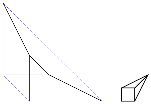
Figure 1. An even primitive tropical curve in a trapezoid $\Delta$ (dashed), corresponding to an immersed Lagrangian sphere in ${\mathbb{C}}{\mathbb{P}}^{2}\#\overline{{\mathbb{C}}{\mathbb{P}}^{2}}$, and its Newton polygon.

The curve $C=\Delta\cap h(\Gamma)$ does not have to be primitive, however we still have a version of Theorem 3.1. As before, we denote the number of codimension 1 boundary points (of boundary momentum 2) with $j$, and the number of ends of $\Gamma_{\Delta}=h^{-1}(\Delta)$ with $\kappa$. Let

$$W=(V_{\Gamma}\cup\Gamma_{\Delta})\cup\bigcup\limits_{w(e)>1}e$$

where the latter union is taken over the edges $e\subset\Gamma_{\Delta}$ of weight greater than one. E.g. in Figure 2 the set $W$ coincides with the edge of weight 2. Note that $W\subset\Gamma_{\Delta}$ and recall that by our assumption an edge of $\Gamma$ of weight greater than one must be disjoint from $\partial\Gamma_{\Delta}=h^{-1}(\partial\Delta)$. For simplicity we assume that $V_{\Gamma}\cap\Gamma_{\Delta}\neq\emptyset$ (note that we did not make such assumption in Theorem 3.1).

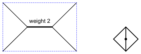
Figure 2. A non-primitive tropical curve in a rectangle for which Theorem 3.2 produces an immersed Lagrangian sphere in ${\mathbb{C}}{\mathbb{P}}^{1}\times{\mathbb{C}}{\mathbb{P}}^{1}$, and its Newton polygon.

Theorem 3.2.

There exists a family of Lagrangian immersions $\nu_{\epsilon}:L\to M_{\Delta}$, for small $\epsilon>0$, where $L$ is a connected smooth surface with $\kappa$ punctures such that $\mu_{\Delta}\circ\nu_{\epsilon}(L)\subset C\cup W_{\epsilon}$.

Furthermore, let $K\subset W$ be a connected component and $Y_{\epsilon}^{K}$ be the $\epsilon$-neighborhood of $h(K)$. We have the following properties.

• The inverse image $(\mu_{\Delta}\circ\nu_{\epsilon})^{-1}(Y_{\epsilon}^{K})\subset L$ contains a unique non-annulus component $L_{K}\subset L$.

• The surface $L_{K}$ is an (open) orientable surface of genus $b_{1}(K)$. The number of ends (punctures) of $L_{K}$ coincides with the number of edges of $\Gamma_{\Delta}$ adjacent to $K$ plus the number of ends of $K$ itself (if any).

• The surface $\nu_{\epsilon}(L_{K})$ has

  $$\delta(K)=\sum\limits_{v\in V_{\Gamma}\cap K}\delta(v)+\sum\limits_{e\in E_{\Gamma\cap K}}(w(e)-1)+\#_{K}(\Sigma(h_{\Delta}))$$

  ordinary $(+1)$-nodes (i.e. transverse double self-intersection points with positive local intersection number with respect to any orientation of $L_{K}$). Here $\#_{K}(\Sigma(h_{\Delta}))$ is the number of pairs $x\neq y\in K$ such that $h(x)=h(y)$, and each such pair is taken with the weight equal to the tropical intersection of the edges $e_{x}\ni x$ and $e_{y}\ni y$, i.e. the absolute value of the scalar product $(dh(e_{x}),dh(e_{y}))$.

A component $B\subset L\smallsetminus\bigcup\limits_{K\subset W}L_{K}$ is an annulus if $\mu_{\Delta}(\nu_{\epsilon}(B))\cap\partial\Delta=\emptyset$, a Möbius band if $\mu_{\Delta}\circ\nu_{\epsilon}(B)$ contains a boundary points of codimension 1, and a disk if $\mu_{\Delta}\circ\nu_{\epsilon}(B)$ contains a boundary points of codimension 2.

This theorem is proved in section 4 along with Theorem 1.

3.2. Example: a real projective plane inside the complex projective plane

Let $\Delta\subset\mathbb{R}^{2}$ be the triangle with vertices $(0,0)$, $(1,0)$ and $(0,1)$, and $C$ be the interval between $(0,0)$ and $(\frac{1}{2},\frac{1}{2})$, see Figure 3.

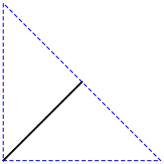
Figure 3. One of the “standard” Lagrangian copies of ${\mathbb{R}}{\mathbb{P}}^{2}$ in ${\mathbb{C}}{\mathbb{P}}^{2}$.

The boundary of $C$ consists of two points, one of codimension 1, and one of codimension 2. The point $(0,0)$ is a bissectrice point while the point $(\frac{1}{2},\frac{1}{2})$ is of boundary momentum 2. We have $V_{C}=\emptyset$. There is only one edge $e\in E_{C}$. In particular, $C$ is smooth.

By Theorem 3.1 there exists a Lagrangian surface diffeomorphic to ${\mathbb{R}}{\mathbb{P}}^{2}$ embedded to $M_{\Delta}={\mathbb{C}}{\mathbb{P}}^{2}$. Note that since $V_{C}=\emptyset$ we have $\mu_{\Delta}(L)=C$ for any small $\epsilon>0$.

A surface of this kind has appeared in [2] for the following property. Consider the interval $I=[(0,a),(1-a,a)]\subset\Delta$ for $0<a<\frac{1}{2}$. Then the restriction of $\omega_{\Delta}$ to $\mu^{-1}_{\Delta}(I)\approx S^{2}\times S^{1}$ is degenerate, and has a 1-dimensional radical direction which defines a $S^{1}$-fibration $\lambda:\mu^{-1}_{\Delta}(I)\to M_{I}={\mathbb{C}}{\mathbb{P}}^{1}\approx S^{2}$. We have $S^{1}\approx Z=L\cap\mu^{-1}_{\Delta}(I)=\{(a,a)\times(y+\Theta_{e})$ according to $(i)$ of Definition 2.1. The restriction $\lambda|_{Z}:Z\to M_{I}={\mathbb{C}}{\mathbb{P}}^{1}$ is an embedding as noted in [2].

More generally (by Lemma 2.3), we have $L\cap\mu^{-1}_{\Delta}(t,t)=\{(t,t)\times(y(t)+\Theta_{e})$, where $y(t)\subset\Theta$ may vary with $t\in[0,\frac{1}{2}]$. If $y(t)=0\in\Theta$ then $L$ is the fixed point locus of the antiholomorphic involution $(z:u:v)\mapsto(\bar{z},\bar{v},\bar{u})$, and thus is a copy of the standard ${\mathbb{R}}{\mathbb{P}}^{2}\subset{\mathbb{C}}{\mathbb{P}}^{2}$ in the homogeneous $(z:x:y)$-coordinates under the linear substitution $u=x+\bar{y}$, $v=\bar{x}+y$.

3.3. Example: tropical wave fronts of planar polyhedral domains

Let $\Delta\subset\mathbb{R}^{2}$ be an arbitrary planar Delzant polyhedral domain, and $\delta>0$ is small. The domain $\Delta$ is the intersection of $N$ of half-planes $\{x\in\mathbb{R}^{2}\ |\ p_{j}(x)\geq a_{j}\}$, $p_{j}\in\mathbb{Z}^{2}$, $a_{j}\in\mathbb{R}$. $j=1,\dots,N$, where $N$ is the number of sides of $\Delta$. Without loss of generality we may assume that $p_{j}$ are primitive (indivisible) vectors in $\mathbb{Z}^{2}$.

Connecting the vertices of the smaller polyhedral domain

$$\Delta_{\delta}=\bigcap\limits_{j=1}^{N}\{x\in\mathbb{R}^{2}\ |\ p_{j}(x)\geq a_{j}+\delta\}$$

with the corresponding vertices of $\Delta$, and taking the union with $\partial\Delta_{\Delta}$ we get an even primitive tropical curve $W_{\delta}\subset\Delta$ such that all the vertices of $\Delta$ are the bissectrice points of $W_{\delta}$, see Figure 4. Since $\Delta$ is assumed to be Delzant, the curve $W_{\delta}$ is smooth for small $\delta>0$.

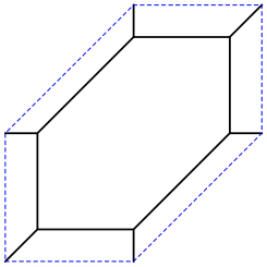
Figure 4. Tropical wave fronts of Delzant domains [8] produce Lagrangian tori in the corresponding toric surfaces (the Del Pezzo surface of degree 6 in the depicted case).

The curve $W_{\delta}$ can be considered as a tropical wave front, and appears in the framework related to Abelian sandpile models in $\Delta$, see [8]. In particular, the evolution of this wave front beyond small values of $\delta$ also produces tropical curves, though perhaps of different combinatorial type.

By Theorem 3.1 $W_{\delta}$ is Lagrangian-realizable by $\Delta$ is Lagrangian-realizable by embedded tori in the case when $\Delta$ is bounded, and by embedded cylinders otherwise.

3.4. Example: Lagrangian embeddings of connected sums of Klein bottles to $\mathbb{C}^{2}$

Recall that $(\mathbb{C}^{2},\frac{i}{2}(dz\wedge d\bar{z}+dw\wedge d\bar{w}))$ is the symplectic toric variety corresponding to the quadrant $\mathbb{R}^{2}_{\geq 0}$. Thus even primitive tropical curves in $\mathbb{R}^{2}_{\geq 0}$ produce Lagrangian immersed surfaces in $\mathbb{C}^{2}$.

All boundary points of the tropical curve

$$C_{3}=[(0,0),(2,2)]\cup[(0,5),(2,2)]\cup[(2,2),(5,0)]\subset\mathbb{R}^{2}_{\geq 0},$$

$k>1$, see Figure 5, are boundary points of codimension 1 and of boundary momenta 2. The curve is not smooth as its only vertex has the self-intersection number equal to 2.

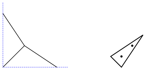
Figure 5. A tropical curve representing an immersed Klein bottle with two nodes and its Newton polygon.

Accordingly we get the following proposition.

Proposition 3.3.

There exists an immersed Lagrangian Klein bottle in $\mathbb{C}^{2}$ with two ordinary self-intersection points.

In a similar way we may construct two series of Lagrangian immersions of connected sum of Klein bottles with growing number of self-intersections.

Proposition 3.4.

For any $k\geq 1$ there exist a Lagrangian immersion of the connected sum of two Klein bottles to $\mathbb{C}^{2}$ with $4k-1$ ordinary self-intersection points.

Proof.

Consider the tropical curve $C_{k}$ obtained as the union of the edges $[(0,3),(2,2k)]$, $[(2,2k),(2+k,0)]$, $[(2,2k),(3,4k-1)]$, $[(0,7k+\frac{1}{2}),(3,4k-1)]$ and $[(3,4k-1),(6k+\frac{3}{2},0)]$. This is an even primitive tropical curve in $\mathbb{R}_{\geq 0}^{2}$ with four boundary vertices of codimension 1, see Figure 6 for $k=1$. If we extend the boundary edges past $\mathbb{R}_{\geq 0}$ as infinite rays we get a tropical curve in $\mathbb{R}^{2}$ with the Newton polygon

$$Q_{k}=\operatorname{ConvexHull}\{(0,-1),(2,2),(-2k+1,0),(-2,-2)\}.$$

The curve $C_{k}$ corresponds to the triangulation obtained by dividing the quadrilateral $Q_{k}$ into two triangles (corresponding to the vertices of $C_{k}$) by the diagonal $[(-2k+1,0),(0,-1)]$, cf. [14]. The two vertices of $C_{k}$ have self-intersection numbers $k$ and $3k-1$, so that Theorem 3.1 produces an immersed Lagrangian surface homeomorphic to the connected sum of Klein bottles with $4k-1$ ordinary self-intersection points. ∎

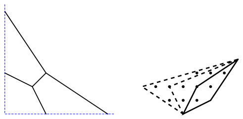
Figure 6. The connected sum of two immersed Klein bottle with $4k-1$ nodes: the tropical curve for $k=1$ and its Newton polygon for $k=1$ (solid polygon) and $k=2,3$ (dashed expansion).

Proposition 3.5.

For any $k\geq 0$ there exist a Lagrangian immersion of the connected sum of three Klein bottles to $\mathbb{C}^{2}$ with $4k$ ordinary self-intersection points.

Proof.

Consider the lattice triangle $N$ with vertices $(-2k-1,0)$, $(4,2)$ and $(-4,-2)$. Consider a subdivision of the triangle $N$ into four triangles by introducing three new vertices $(-2,-1)$, $(0,0)$ and $(2,1)$ at the edge $[(4,2),(-4,-2)]$, see Figure 7.

Figure 7. Newton polygons and their subdivisions for Lagrangian immersions of the connected sum of three Klein bottles with $4k$ nodes for $k=1$ and $k=2$.

The resulting triangulation is convex in the sense of Viro patchworking [23]. Thus there exists a tropical curve $C\subset\mathbb{R}^{2}$ dual to it, see [14]. By our choice of the subdivision we have $b_{1}(C)=0$. The leaves of $C$ are orthogonal to the edges of the triangle $N$ serving as the Newton polygon of $C\subset\mathbb{R}^{2}$. Namely, we have a leaf in the direction of $(-2,2k+5)$, a leaf in the direction $(-2,3-2k)$, and four leaves in the direction $(1,-2)$.

Translating $C$ sufficiently high up in the direction of $(1,t)$ where $0<t<\frac{2}{2k-3}$ ensures that the first two leaves intersect the $y$-axis of $\mathbb{R}^{2}_{\geq 0}$ while the last four leaves intersect the $y$-axis of the translation so that all boundary momenta are 2. The proposition now follows from Theorem 3.2. ∎

Smoothing all ordinary nodes of Lagrangian immersions from Propositions 3.3-3.5 we recover proof of the following theorem of Givental.

Corollary 3.6 ([6]).

There exist Lagrangian embeddings of surfaces diffeomorphic to $2k+1$ copies of the Klein bottle to $\mathbb{C}^{2}$, $k\geq 1$.

Remark 3.7.

Another construction of Lagrangian embeddings of $2k+1$ copies of the Klein bottle to $\mathbb{C}^{2}$, $k\geq 1$, can be given by Lagrangian surgery of an immersed Lagrangian spheres with $2k+1$ self-crossings (out of these $k+1$ must be positive and $k$ must be negative). The presence of negative crossing makes the result of the surgery non-orientable.

By the methods of this paper it is not clear if one can further degenerate the surfaces given by Corollary 3.6 to obtain such an immersed sphere. It might be interesting to detect whether this deformation exist or Corollary 3.6 gives a different example of embedded connected sums of Klein bottles.

4. Proof of Theorem 1

Consider the hyperkähler twist

$$\operatorname{HT}:(\mathbb{C}^{\times})^{2}\to(\mathbb{C}^{\times})^{2},\ (e^{x_{1}+iy_{1}},e^{x_{2}+iy_{2}})\mapsto(e^{x_{1}-iy_{2}},e^{x_{2}+iy_{1}})$$

in $(\mathbb{C}^{\times})^{2}$.

Lemma 4.1.

If $V\subset(\mathbb{C}^{\times})^{2}$ is an immersed holomorphic curve then $\operatorname{HT}(V)\subset(\mathbb{C}^{\times})^{2}$ is an immersed Lagrangian with respect to

$$\omega_{(\mathbb{C}^{\times})^{2}}=\frac{i}{2}(\frac{dz_{1}}{z_{1}}\wedge\frac{d\bar{z}_{1}}{\bar{z}_{1}}+\frac{dz_{2}}{z_{2}}\wedge\frac{d\bar{z}_{2}}{\bar{z}_{2}})=dx_{1}\wedge dy_{1}+dx_{2}\wedge dy_{2}.$$

Proof.

The holomorphic 2-form $(dx_{1}+idy_{1})\wedge(dx_{2}+idy_{2})$ must vanish on any tangent space to a holomorphic curve $V$. Therefore, the form $(dx_{1}+idy_{2})\wedge(dx_{2}-idy_{1})=(dx_{1}\wedge dx_{2}-dy_{1}\wedge dy_{2})-i(dx_{1}\wedge dy_{1}+dx_{2}\wedge dy_{2})$ vanishes on any tangent space to $\operatorname{HT}(V)$. In particular, the imaginary part on this form vanishes. ∎

It is convenient for us to use two systems of coordinates: the multiplicative holomorphic coordinates $(z_{j})_{j=1}^{n}\in(\mathbb{C}^{\times})^{n}$ and the additive real coordinates $(x_{j},y_{j})_{j=1}^{n}\in(\mathbb{R}\times(\mathbb{R}/2\pi\mathbb{Z}))^{n}$, $z_{j}=e^{x_{j}+iy_{j}}$. For $t>0$ the scaling map

(10) $$\operatorname{sc}_{t}(x_{j},y_{j})=(tx_{j},y_{j})$$

is a diffeomorphism of $(\mathbb{C}^{\times})^{n}$ rescaling the symplectic form $\omega=\sum\limits_{j=1}^{n}dx_{j}\wedge dy_{j}$. In particular, it sends Lagrangian varieties to Lagrangian varieties.

Lemma 4.2.

Theorem 1 holds in the case if $\Delta=\mathbb{R}^{2}$ and $C\subset\mathbb{R}^{2}$ is a tropical line, i.e. $C=Y$ for the union $Y\subset\mathbb{R}^{2}$ of three rays from $0\in\mathbb{R}^{2}$ in the direction $(-1,0)$, $(0,-1)$ and $(1,1)$.

Proof.

The line $V=\{(z_{1},z_{2})\in(\mathbb{C}^{\times})^{2}\ |\ z_{1}+z_{2}-1=0\}$ is holomorphic. Thus $\operatorname{HT}(V)$ as well as $S_{t}=\operatorname{sc}_{t}(\operatorname{HT}(V))$ are Lagrangians, $t>0$. In particular, $\mu(S_{t})$ is contained in the $\epsilon$-neighborhood $U_{\epsilon}(Y)\supset Y$ for sufficiently small $t$.

The three rays of $Y$ are symmetric with respect to $GL_{2}(\mathbb{Z})$, so it suffices to deform $S_{t}$ into $S^{\prime}_{t}$ in the class of Lagrangians within $\mu^{-1}(U_{\epsilon}(Y))$ so that $\mu(S_{t})\cap\{x_{1}<-\epsilon/2\}=\{x_{2}=0\}\cap\{x_{1}<-\epsilon/2\}$.

But for small $t>0$ over $\{x_{1}<-\epsilon/2\}$ the Lagrangian surface $S_{t}$ is approximated by

$$Z_{0}=\operatorname{HT}(\{z_{2}-1=0\})=\operatorname{HT}(\{x_{2}=0,y_{2}=0\})=\{x_{2}=0,y_{1}=0\}$$

since at $z_{1}=0$ the equation $z_{1}+z_{2}-1=0$ degenerates to $z_{2}=-1=0$.

By the Darboux theorem, a small neighborhood of $Z_{0}$ in $(\mathbb{C}^{\times})^{2}$ is symplectomorphic to a small neighborhood in its cotangent bundle (with the standard symplectic structure $dp\wedge dq$). Thus any surface approximating $Z_{0}$ is given by a small 1-form $\alpha$ on $Z_{0}$. As $S_{t}$ is Lagrangian, we have $d\alpha=0$. Furthermore, $\alpha$ is exact if and only if $\int\limits_{\gamma}\alpha=0$ for a loop $\gamma$ realizing non-trivial homology class in $H_{1}(Z_{0})\approx\mathbb{Z}$.

Taking $\gamma=Z_{0}\cap\{|z_{1}|=s\}$ for arbitrary small $s>0$ we see that $|\int\limits_{\gamma}\alpha|$ must be arbitrary small itself. Thus $\int\limits_{\gamma}\alpha=0$, and so $\alpha=df$ for a smooth function $f:Z_{0}\to\mathbb{R}$. Using the partition of unity we deform $f$ to a smooth function $f^{\prime}:Z_{0}\to\mathbb{R}$ such that $f^{\prime}(x_{1},x_{2},y_{1},y_{2})=f$ if $x_{1}>-3\epsilon/4$, and $f^{\prime}(x_{1},x_{2},y_{1},y_{2})=0$ if $x_{1}<-\epsilon$, and set $S^{\prime}_{t}$ to be the surface defined by $f^{\prime}$. ∎

Corollary 4.3.

Theorem 1 holds if $\Delta=\mathbb{R}^{2}$ and $C\subset\mathbb{R}^{2}$ has a single vertex.

Proof.

Since $C$ is trivalent, there exist an affine map $\rho:\mathbb{R}^{2}\to\mathbb{R}^{2}$ and a multiplicative-affine map $\rho_{\mathbb{C}}:(\mathbb{C}^{\times})^{2}\to(\mathbb{C}^{\times})^{2}$ such that $\mu\circ\rho_{\mathbb{C}}=\rho\circ\mu$ and $C=\rho(Y)$. Here $\rho$ (resp. $\rho_{\mathbb{C}}$) is a composition of an integer linear map in $\mathbb{R}^{2}$ (resp. in $(\mathbb{C}^{\times})^{2}$) and a translation in $\mathbb{R}^{2}$ (resp. in $(\mathbb{C}^{\times})^{2}$) of determinant (resp. degree) equal to the multiplicity of the vertex $v\in C$, see Lemma 8.21 of [14].

The image $\rho_{\mathbb{C}}(S_{t})$ is a rational curve with three punctures of the same Newton polygon as the tropical curve $C\subset\mathbb{R}^{2}$, i.e. a pair-of-pants. Thus it has arithmetic genus $\delta(v)$ which correspond to $\delta(v)$ ordinary nodes by Corollary 8.20 of [14]. We set $L=\rho_{C}(S^{\prime}_{t})$ for small $t>0$ and $S^{\prime}_{t}$ from the proof of Lemma 4.2. ∎

Lemma 4.4.

Let $E_{j}\in\mathbb{R}^{n}$, $j=1,2$, be two disjoint open intervals parallel to the same integer vector $u\in\mathbb{Z}^{n}$ and $L_{j}\subset(\mathbb{C}^{\times})^{n}$ be two smooth connected Lagrangian varieties such that $\mu(L_{j})\subset E_{j}$, and $L_{j}$ is relatively closed in $\mu^{-1}(E_{j})$.

There exists a Lagrangian variety $L\subset(\mathbb{C}^{\times})^{n}$ diffeomorphic to $\mathbb{R}\times(S^{1})^{n-1}$ such that $L_{1}$ and $L_{2}$ are its subvarieties if and only if $E_{1}$ and $E_{2}$ belong to the same line $E\subset\mathbb{R}^{n}$. Furthermore, if $E_{1},E_{2}\subset E$ then the Lagrangian variety $L\supset L_{1},L_{2}$ can be chosen so that $\mu(L)\subset E$.

Proof.

Without loss of generality we may assume that $E_{j}$ are parallel to $(1,0,\dots,0)$. If $E_{1}$ and $E_{2}$ do not belong to the same line then without loss of generality we may also assume that the $x_{2}$-coordinates of $E_{1}$ and $E_{2}$ are different. By Lemma 2.3, both $L_{1}\cup L_{2}$ contain $x\times\Theta_{E}$ for any $x\in E_{1}\cup E_{2}$, where $\Theta_{E}\subset\Theta=(\mathbb{R}/2\pi)^{n}$ is the $(n-1)$-dimensional subtorus conormal to $E$.

Let $I=[a_{1},a_{2}]\subset\mathbb{R}^{n}$ be an interval connecting $E_{1}$ and $E_{2}$. By Lemma 2.3, $\mu^{-1}(a_{j})=\{a_{j}\}\times(y_{a_{j}}+\Theta_{E})$. Choose a smooth function $I\ni a\mapsto y_{a}\in\Theta=(\mathbb{R}/2\pi\mathbb{Z})^{n}$, and consider the cylinder

$$W=\{\{a\}\times(y_{a}+\Theta_{2})\ |\ a\in I\}\subset(\mathbb{C}^{\times})^{n}.$$

Here $\Theta_{2}\subset\Theta$ is a circle given by $y_{k}=0$, $k\neq 2$. Note that the symplectic area of this cylinder is equal to $2\pi$ times the difference between the $x_{2}$-coordinates of $E_{1}$ and $E_{2}$.

Suppose that there exists $L\supset L_{1},L_{2}$ with $H_{1}(L)\approx\mathbb{Z}$. Then the two components of $\partial W$ must be homologous in $L$ and thus the area of $W$ must vanish.

On the other hand, if $E_{1},E_{2}\subset E$ then we obtain $L$ by extending the smooth function $E_{1}\mapsto E_{2}\ni a\mapsto y_{a}\in\Theta$ to $E$. ∎

Remark 4.5.

The Lemma above is related to the Menelaus theorem, in particular, to its tropical version, see [16] for the case $n=2$. Namely, let $L\subset(\mathbb{C}^{\times})^{2}$ be a properly immersed oriented Lagrangian surface with finitely many ends. For every end $F$ of $L$ we may take a loop $\gamma_{F}$ going around $F$ in the positive direction. We can define the momentum $m(F)$ of $F$ to be the integral of the symplectic form $\omega$ against a membrane connecting $\gamma$ to a loop in the Lagrangian torus $\mu^{-1}(0)$. It is easy to see that the momenta of $L$ coincide with the momenta of the corresponding ends of the tropical curve, and thus the next proposition corresponds to Proposition 6.12 of [16].

Proposition 4.6 (Lagrangian Menelaus theorem).

We have

$$\sum\limits_{F}m(F)=0,$$

where the sum is taken over the ends of all ends of a properly immersed Lagrangian surface $L$ in $(\mathbb{C}^{\times})^{2}$.

Proof.

The union of all $\gamma_{F}$ is homologous to zero. Thus the union of all membranes for $\gamma_{f}$ can be completed by a Lagrangian chain (contained in the union of $L$ and $\mu^{-1}(0)$) to a closed surface in $(\mathbb{C}^{\times})^{2}$. But the integral of $\omega$ against any closed surface in $(\mathbb{C}^{\times})^{2}$ is zero. ∎

Proof of Theorem 1.

Let $C\subset\Delta$ be an even primitive tropical curve and $v\in V_{C}$. The tripod $Y_{v}\subset A_{v}$ obtained as the union of $v$ with the three rays from $v$ obtained by extending the edges of $C$ adjacent to $v$ indefinitely is a primitive tropical curve in the tropical affine plane $A_{v}\approx\mathbb{R}^{2}$. Thus $Y_{v}\subset A_{v}$ is Lagrangian-realizable by Corollary 4.3. Let $Q_{v}$ be the corresponding Lagrangian realization for $\epsilon/2>0$ restricted to $\mu^{-1}(U_{\epsilon}(v))$. It is an immersed isotropic pair-of-pants surface (which becomes half-dimensional, and thus Lagrangian once we restrict the ambient space to a complex monomial subsurface of $(\mathbb{C}^{\times})^{n}$ corresponding to $B$).

Consider the $(n-2)$-torus $\Theta_{v}$ conormal to all three edges of $C$ adjacent to $v$. Then $Q_{v}\times\Theta_{v}$ gives an immersed Lagrangian variety $L_{v}$ in $\mu^{-1}(U_{\epsilon}(v))$ such that $\mu(L_{v})\cap(U_{\epsilon}(v)\smallsetminus U_{\frac{\epsilon}{2}}(v)$ is contained in $C$. We use Lemma 4.4 for each bounded edge $[v,v^{\prime}]\in E_{C}$ to join $L_{v}$ and $L_{v^{\prime}}$ to a single Lagrangian.

To finish the proof of the theorem we need to construct $L$ over the neighborhoods of boundary points of $C$. If $w\in\partial\Delta$ is a boundary point we consider its $\epsilon$-neighborhood $I_{\epsilon}(w)\approx[0,\epsilon)$ in $C$ and set $L_{w}$ to be the closure of $(I_{\epsilon}(w)\smallsetminus\{w\})\times\Theta_{w}$, where $\Theta_{w}$ is the $(n-1)$-dimensional subtorus of $\Theta=(\mathbb{R}/2\pi\mathbb{Z})^{n}$ conormal to $I_{\epsilon}(w)$. If $w$ is a boundary point of codimension 1 and boundary momentum 1 then $L_{w}$ is a smoothly embedded non-orientable Lagrangian variety diffeomorphic to the Möbius band times $(S^{1})^{n-2}$.

If $w$ is a bissectrice point and $\Delta=(\mathbb{R}_{\geq}0)^{2}$ then locally $C$ must coincide with the diagonal ray $x_{1}=x_{2}$. Thus the Lagrangian $L_{w}$ is a smooth disk that can be obtained from the complex disk contained in $\{z_{1}=z_{2}\}$ as the image of the map $\operatorname{HT}$. In the general case $L_{w}$ is the product of this disk and $(S^{1})^{n-2}$. ∎

Proof of Theorem 3.2.

Suppose that $\Delta\subset\mathbb{R}^{2}$, but $C\subset\Delta$ is allowed to have edges of multiple edge not adjacent to $\partial\Delta$. The proof is similar to the proof of Theorem 1, but instead of patching pairs-of-pants over neighborhoods of vertices of $C$ we patch together Lagrangian surfaces over the components of $W$ constructed in the following way. Let $K\subset W$ be such a component. Extend all edges adjacent to $K$ indefinitely as rays in $\mathbb{R}^{2}$. The result is a tropical curve. Its approximation by holomorphic curves is provided by Lemma 8.4 of [14] once we choose a marked point at all but one leaf of that curve. To finish the proof we apply the map $\operatorname{HT}$ to the approximating curves. ∎

5. More background material: tropical enumerative problems and multiplicity

5.1. Regular tropical curves

Given a tropical immersion $h:\Gamma\to A$ we may choose a reference vertex $v\in V_{\Gamma}$, and deform $h$ as follows. We may deform the tropical structure on $\Gamma$, i.e. vary the lengths of its bounded edges. Such deformation results in a tropical curve $\Gamma^{\prime}$ homeomorphic to $\Gamma$, but with different lengths of bounded edges. A tropical immersion $h^{\prime}:\Gamma^{\prime}\to A$ with $h^{\prime}(v)=h(v)$ and $dh(e)=dh^{\prime}(e)$ for all oriented edges $e\in E_{\Gamma}$ exists if and only if

(11) $$\sum\limits_{e\in Z}dh(e)l(e)=0\in\Lambda$$

for every oriented cycle $Z\subset\Gamma$.

The space of all possible tropical structures on $\Gamma$ is $\mathbb{R}_{\geq 0}^{b}$, where $b$ is the number of bounded edges of $\Gamma$. The corresponding deformations of $h:\Gamma\to A$ keeping the value $h(v)\in A$ are a subspace $\operatorname{Def}_{v}(h)\subset\mathbb{R}_{>0}^{b}$ by the linear equations (11) for a system of $b_{1}(\Gamma)$ homologically independent cycles $Z$.

Definition 5.1.

A topological immersion $h:\Gamma\to\mathbb{R}^{n}$ is called regular if the codimension of $\operatorname{Def}_{v}(h)$ is $nb_{1}(\Gamma)$, i.e. the conditions (11) for homologically independent cycles $Z$ are linearly independent.

Also we may deform $h(v)\in A$ without changing the tropical structure. This amounts to composing $h:\Gamma\to A$ with the translation by an element of $\Lambda\otimes\mathbb{R}$ in $A$. If $\Gamma$ is 3-valent then any small deformation of $h$ is a combination of a deformation inside $\operatorname{Def}_{v}(h)$ and a translation in $A$. Thus locally the space $\operatorname{Def}(h)$ of all deformations of $h$ is a linear space $\operatorname{Def}_{v}(h)\times(\Lambda\otimes\mathbb{R})$. Note that since (11) are linear equations in $l(e)$ with integer coefficients, the subspace $\operatorname{Def}_{v}(h)\subset\mathbb{R}^{b}_{>0}$ is defined over $\mathbb{Z}$.

From now on we assume that the graph $\Gamma$ with $\kappa$ ends is 3-valent, so that $b=\kappa-3+3b_{1}(\Gamma)$. The space $\operatorname{Def}(h)=\operatorname{Def}_{v}(h)\times(\Lambda\otimes\mathbb{R})$ is a convex open set in a tropical affine space $\mathbb{R}^{b}\times\mathbb{R}^{n}$ of dimension

$$a=\dim\mathbb{R}^{b}\times\mathbb{R}^{n}\geq b-nb_{1}(\Gamma)+n=\kappa+(n-3)(1-b_{1}(\Gamma)).$$

The right-hand side is the expected dimension of $\operatorname{Def}(h)$ which agrees with the expected dimension of the space of deformations of a classical curve of genus $g$ in an $n$-fold where the value of the first Chern class on this curve is equal to $\kappa$. One may also note that in any toric compactification of $\mathbb{R}^{n}$ the first Chern class is represented by the union of divisors at infinity, and so $\kappa$ indeed corresponds to the value of the first Chern class in the case if the weights of all the leaves of $h:\Gamma\to\mathbb{R}^{n}$ are 1.

Remark 5.2.

We say that $h:\Gamma\to\mathbb{R}^{n}$ is a rational tropical curve in $\mathbb{R}^{n}$ if $b_{1}(\Gamma)=0$, i.e. $\Gamma$ is a tree. Clearly any such curve is regular as the codimension in $\mathbb{R}^{b}\times\mathbb{R}^{n}$ is tautologically zero.

Theorem 1 of [15] claims that all regular tropical curves are classically realizable. The survey [15] did not contain any proofs, but various versions of tropical-to-complex correspondences for regular curves had appeared in [14], [20], [21], [18], [22], [17], [11] (the list is not exhaustive). This correspondence is particularly useful for studying some classical enumerative problems on the number of curves of given degree and genus passing through a number of constraints. For the purposes of this paper we are interested in the example of a tropical enumerative problem considered in the next subsection. In particular, in the remaining part of the paper we restrict our attention to rational tropical curves.

5.2. A tropical enumerative problem in $\mathbb{R}^{3}$ (an example).

Consider the following example of a tropical enumerative problem in $\mathbb{R}^{3}$. Let $\mathcal{D}=\{d_{j}\}_{j=1}^{\kappa}$, $u_{j}\in\mathbb{Z}^{3}$, $\kappa\in\mathbb{N}$, be a collection of non-zero integer vectors such that $\sum\limits_{j=1}^{\kappa}d_{j}=0$. Such a collection $\mathcal{D}$ is called a toric degree. We say that a (rational) tropical curve $h:\Gamma\to\mathbb{R}^{3}$ is of degree $\mathcal{D}$ if $dh(e_{j})=d_{j}$ for some ordering of the leaves $\{e_{j}\}$, $j\in 1,\dots,\kappa$. We denote the space of all rational tropical curves of toric degree $\mathcal{D}$ with ${\mathcal{M}}_{\mathcal{D}}$.

Let $\mathcal{Z}=\{\mathfrak{z}_{j}\}_{j=1}^{\kappa}$ $\mathfrak{z}_{j}\in\mathbb{Z}^{3}$ be another collection of non-zero integer vectors, this time without an extra conditions on the sum. Consider a configuration $\mathfrak{L}=\{\mathfrak{l}_{j}\}_{j=1}^{\kappa}$ of lines $\mathfrak{l}_{j}\subset\mathbb{R}^{3}$ such that $\mathfrak{l}_{j}$ is parallel to $\mathfrak{z}_{j}$. We say that a tropical curve $h:\Gamma\to\mathbb{R}^{3}$ passes through $\mathfrak{L}$ if $h^{-1}(\mathfrak{l}_{j})\neq\emptyset$ for every $j=1,\dots,\kappa$.

Let $\mathcal{E}=\{e_{j}\}_{j=1}^{\kappa}$, $e_{j}\in E_{\Gamma}$, be a collection of edges of $\Gamma$ (maybe with repetitions). We say that $h:\Gamma\to\mathbb{R}^{3}$ passes through $\mathfrak{L}$ at $\mathcal{E}$ if $h^{-1}(\mathfrak{l}_{j})\cap e_{j}\neq\emptyset$ for every $j=1,\dots,\kappa$.

For the collection $\mathcal{Z}$ we denote the space of all compatible configurations $\mathfrak{L}$ with ${\mathcal{M}}(\mathcal{Z})$. Clearly, ${\mathcal{M}}(\mathcal{Z})\approx(\mathbb{R}^{2})^{\kappa}$ is an affine space over a vector space of dimension $2\kappa$. Thus we may speak of generic configurations $\mathfrak{L}$.

Definition 5.3.

We say that $h:\Gamma\to\mathbb{R}^{3}$ and $h^{\prime}:\Gamma^{\prime}\to\mathbb{R}^{3}$ are of the same combinatorial type if there exists a homeomorphism $\Phi:\Gamma\to\Gamma^{\prime}$ that sends an oriented edge $e\in E_{\Gamma}$ to an oriented edge $e^{\prime}\in E_{\Gamma^{\prime}}$ so that $dh(e)=dh^{\prime}(e^{\prime})\in\mathbb{Z}^{3}$. We have denoted the combinatorial type of $h$ with $\operatorname{Def}(h)$.

Clearly, there are finitely many combinatorial types of curves of a given toric degree passing through $\mathfrak{L}$ at $\mathcal{E}$.

Lemma 5.4.

If $\mathfrak{L}$ is chosen generically in ${\mathcal{M}}(\mathcal{Z})$ then there is at most one curve in the combinatorial type of a tropical rational curve of toric degree $\mathcal{D}$ passing through $\mathfrak{L}$ at $\mathcal{E}$.

Furthermore, if a tropical curve $h:\Gamma\to\mathbb{R}^{3}$ passes through $\mathfrak{L}$ then $\Gamma$ of $h$ is 3-valent, and the inverse image $h^{-1}(\mathfrak{l}_{j})$ is finite and disjoint from $V_{\Gamma}$. In addition we have $dh(e)\neq 0$ for any $e\in E_{\Gamma}$.

Proof.

By regularity of rational tropical curves we have $\dim\operatorname{Def}(h)\leq\kappa$, and $\dim\operatorname{Def}(h)<\kappa$ unless $\Gamma$ is 3-valent. For a vertex $v\in V_{\Gamma}$ consider the map $\operatorname{ev}_{v}:\operatorname{Def}(h)\to\mathbb{R}^{3}$ defined by $\operatorname{ev}_{v}(h)=h(v)$. For an edge $e\in E_{\Gamma}$ define the space $\mathbb{R}^{3}/dh(e)\approx\mathbb{R}^{2}$ as the quotient of $\mathbb{R}^{3}$ by the subspace generated by the vector $dh(e)$ if it is non-zero and as $\mathbb{R}^{3}/dh(e)=\mathbb{R}^{3}$ if $dh(e)=0$. Define the map

(12) $$\operatorname{ev}_{e}:\operatorname{Def}(h)\to\mathbb{R}^{3}/dh(e)$$

by setting $\operatorname{ev}_{e}(h^{\prime})$, $h^{\prime}\in\operatorname{Def}(h)$, to be the image of the edge $h^{\prime}(e)$ under the projection $\mathbb{R}^{3}\to\mathbb{R}^{3}/dh(e)$. Clearly, these are linear maps on $\operatorname{Def}(h)\subset\mathbb{R}_{>0}^{b}\times\mathbb{R}^{3}$. The lemma now follows from computing dimensions once we note that if $dh(e^{\prime})=0$ for an edge $e^{\prime}$ then the map $\operatorname{Def}(h)\to\mathbb{R}^{3}/dh(e)$ has a kernel corresponding to varying of the length of $e^{\prime}$ for any $e\in E_{\Gamma}$. ∎

Corollary 5.5.

There is a finite set ${\mathcal{M}}(\mathcal{D},\mathfrak{L})$ of rational tropical curves of toric degree $\mathcal{D}$ passing through $\mathfrak{L}$ as long as $\mathfrak{L}$ is generic.

For every $h:\Gamma\to\mathbb{R}^{3}$ such that $h^{-1}(\mathfrak{l}_{j})\cap e_{j}\neq 0$ define

(13) $$\operatorname{ev}_{\mathcal{E}}:\operatorname{Def}(h)\to\mathbb{R}^{l}$$

as the direct sum of the maps sending $h^{\prime}\in\operatorname{Def}(h)$ to the mixed product of $d_{j}$, $\mathfrak{z}_{j}$ and any vector connecting a point of $h(e_{j})$ and a point of $\mathfrak{l}_{j}$. The curve $h:\Gamma\to\mathbb{R}^{3}$ passes through $\mathfrak{L}$ at $\mathcal{E}$ if and only if $\operatorname{ev}_{\mathcal{E}}=0$. The map $\operatorname{ev}_{\mathcal{E}}$ is linear and defined over $\mathbb{Z}$.

The multiplicity $m(h,\mathcal{E},\mathfrak{L})$ of a tropical curve $h$ passing through $\mathfrak{L}$ at $\mathcal{E}$ is the absolute value of the determinant of $\operatorname{ev}_{e}$. We set

$$m(h,\mathfrak{L})=\sum\limits_{\mathcal{E}}m(h,\mathcal{E},\mathfrak{L}),$$

where the sum is taken over all possible configuration of edges $\mathcal{E}=\{e_{j}\}$, $e_{j}\in E_{\Gamma}$, $j=1,\dots,k$, with $h^{-1}(\mathfrak{l}_{j})\cap e_{j}\neq\emptyset$. The number

(14) $$m(\mathcal{D},\mathfrak{L})=\sum\limits_{h\in{\mathcal{M}}(\mathcal{D},\mathfrak{L})}m(h,\mathfrak{L})$$

is the number of tropical curves passing through $\mathfrak{L}$.

It can be shown that $m(\mathcal{D},\mathfrak{L})$ depends only on $\mathcal{D}$ and $\mathcal{Z}$ (recall that $\mathfrak{L}$ is chosen generically). In particular, this claim follows from the correspondence with the number of complex curves in $(\mathbb{C}^{\times})^{3}$ of toric degree $\mathcal{D}$ passing through an appropriate collection of monomial curves defined by $\mathcal{Z}$ which is a special case of [18].

6. Rational tropical curves and three-dimensional Lagrangians

6.1. A vector product formula for the tropical multiplicity $m(h,\mathfrak{L})$

In this subsection we compute the multiplicity $m(h,\mathfrak{L})$ from (14) for a rational 3-valent tropical curve $h:\Gamma\to\mathbb{R}^{3}$ of toric degree $\mathcal{D}$ passing through a generic configuration $\mathfrak{L}$ of lines $\mathfrak{l}_{j}\subset\mathbb{R}^{3}$ parallel to a collection $\mathcal{Z}=\{\mathfrak{z}_{j}\in\mathbb{Z}^{3}\}$, $j=1,\dots,\kappa$ in a special case of the so-called boundary configuration.

Definition 6.1.

We say that $\mathfrak{L}$ is a boundary configuration for $h$ if for every $j=1,\dots,\kappa$ there exists a leaf (unbounded edge) $e_{j}\subset\Gamma$ such that $h^{-1}(\mathfrak{l}_{j})$ is a point contained in $e_{j}$ and $e_{j}\neq e_{k}$ if $j\neq k$.

For the rest of the section we assume that $\mathfrak{L}$ be a boundary configuration for $h$. Recall that $d_{j}=dh(e_{j})\in\mathbb{Z}^{3}$ is the image of a unit tangent vector to the edge $e_{j}$ under the differential of $h$.

Definition 6.2.

The leaf rotational momentum

$$\rho_{j}=d_{j}\times\mathfrak{z}_{j}\in\mathbb{Z}^{3}$$

is the vector product of $u_{j}$ and $\mathfrak{z}_{j}$. Like the vectors $u_{j}$ and $\mathfrak{z}_{j}$ themselves, it is well-defined up to sign.

The tree $\Gamma$ with the leaf $e_{\kappa}$ chosen as the root encodes a way to place parentheses for the binary operation on the leaves $e_{1},\dots,e_{\kappa-1}$. Namely, $\Gamma$ is oriented towards the root, and the orientation determines the order of binary operations, see Figure 8. We start with the rotational momenta at the leaves $e_{1},\dots,e_{\kappa-1}$. At every vertex of $\Gamma$ we have two incoming edges $\iota_{1},\iota_{2}\in E_{\Gamma}$, and an outgoing edge $o\in E_{\Gamma}$.

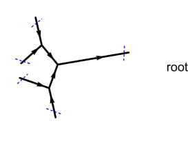
Figure 8. A tropical curve trough a boundary configuration of lines (shown by dashed intervals) and the order of binary operations determined by a choice of the root.

If the rotational momenta for the incoming edges are already defined then we define the rotational momentum for the outgoing edge as

(15) $$\rho(o)=(\rho(\iota_{1})\times\rho(\iota_{2}))\times(dh(o)),$$

i.e. the vector product of the rotational momenta of the incoming edges followed by the vector product with the image of a unit vector to the outgoing edge. The vector $\rho(o)$ is well-defined up to sign as we do not have a preferred order for the incoming edges, but so are the rotational momenta for the incoming edges.

Remark 6.3.

Presence of the triple vector product in (15) is related to our usage of a vector product which depends on the scalar product in $\mathbb{R}^{3}$ that is not canonical for our problem. However, thanks to the double appearance of the vector product operation, the result depends only on the volume form in $\mathbb{R}^{3}=\mathbb{Z}^{3}\otimes\mathbb{R}$ that is naturally associated with the tropical structure, cf. Remark 6.8. Namely, the image of the unit vector $dh(o)$ and the rotational momenta $\rho(\iota_{j})$ belong to dual vector spaces. More canonically, we may replace the vector product with the wedge product followed by the isomorphism to the dual space (cf. (18)), so that the image of $\rho(\iota_{1})\wedge\rho(\iota_{2})$ and $dh(o)$ belong to the same (dual) vector space. Taking their wedge product followed by the isomorphism back to the original space we obtain the rotational momentum $\rho(o)$ from the same vector space as $\rho(\iota_{j})$.

Starting from $\rho(e_{j})$, $j=1,\dots,\kappa-1$, and applying (15) at all vertices we obtain the rotational momentum $\rho(e_{\kappa})$.

Definition 6.4.

The mixed $h$-product

$$(\mathfrak{z}_{1},\dots,\mathfrak{z}_{\kappa})_{h}=\rho(e_{\kappa}).\rho_{\kappa}$$

of rotational momenta of $\mathcal{Z}$ along $h:\Gamma\to\mathbb{R}^{3}$ is the scalar product of $\rho_{\kappa}$ and $\rho(e_{\kappa})$. It is well-defined up to sign.

Example 6.5.

If $\Gamma$ is a tripod then $\kappa=3$ and

$$(\mathfrak{z}_{1},\mathfrak{z}_{2},\mathfrak{z}_{3})_{h}=\pm(\rho_{1},\rho_{2},\rho_{3})\in\mathbb{Z}^{3}$$

is the mixed product of the rotational momenta $\rho_{1},\rho_{2},\rho_{3}\in\mathbb{Z}^{3}$.

Lemma 6.6.

The $h$-product $(\mathfrak{z}_{1},\dots,\mathfrak{z}_{\kappa})_{h}$ does not depend on the choice of the root leaf $e_{\kappa}$ and thus on the order of $\mathfrak{z}_{1},\dots,\mathfrak{z}_{\kappa}$.

Proof.

It is convenient to allow a 3-valent vertex $v\in\Gamma$ to be a root as well. We have the binary operations for rotational momenta as before for edges with two input and one output vertices. At $v$ we have three input vertices and perform the mixed product.

By the property of the mixed product of three vectors in $\mathbb{R}^{3}$ the result (up to sign) is invariant under all permutations of these vectors. This implies that the mixed $h$-product stays invariant if we change the root from a leaf to its adjacent 3-valent vertex, or from a 3-valent vertex to an adjacent 3-valent vertex. ∎

Proposition 6.7.

The absolute value $|(\mathfrak{z}_{1},\dots,\mathfrak{z}_{\kappa})_{h}|$ coincides with the multiplicity $m(h,\mathfrak{L})$.

Proof.

The proposition amounts to computing the determinant of the map (13) in the case when $\Gamma$ is a trivalent tree, and the line $\mathfrak{l}_{j}$ intersects the leaf $e_{j}$ of $\Gamma$. We do it by induction on the number of vertices of $\Gamma$.

If $\Gamma$ has a single 3-valent vertex then $\operatorname{Def}(h)$ can be identified with translations in $\mathbb{R}^{3}$. The coordinates of $\operatorname{ev}_{\mathcal{E}}$ are given by the rotational momentum of the leaves $e_{j}$. Thus the proposition in this case follows from the interpretation of the (classical) triple mixed product as the determinant of the parallelepiped built on the vectors.

Let $\Gamma$ be a tree with at least two 3-valent vertices, and $p\in\Gamma$ be a point inside a bounded edge $e$ of $\Gamma$. The complement $\Gamma\smallsetminus\{p\}$ consists of two components. Extending their edges adjacent to $p$ indefinitely to rays $r_{j}$ we obtain two rational 3-valent tropical curves $h_{j}:\Gamma_{j}\to\mathbb{R}^{3}$, $j=1,2$, with the property that $h(r_{1})$ and $h(r_{2})$ are contained in the same line of $\mathbb{R}^{3}$. We get a linear inclusion map $\operatorname{Def}(h)\to\operatorname{Def}(h_{1})\times\operatorname{Def}(h_{2})$ with the image given as the pull-back of the diagonal in $(\mathbb{R}^{3}/dh(e))\times(\mathbb{R}^{3}/dh(e))$ under the map

$$\operatorname{ev}_{r_{1}}\times\operatorname{ev}_{r_{2}}:\operatorname{Def}(h_{1})\times\operatorname{Def}(h_{2})\to(\mathbb{R}^{3}/dh(e))\times(\mathbb{R}^{3}/dh(e))=E\times E.$$

The vector space $E=(\mathbb{R}^{3}/dh(e))\approx\mathbb{R}^{2}$ is by construction defined over integers. Denote the underlying integer lattice with $\Lambda_{E}\approx\mathbb{Z}^{2}$.

The generator $\Lambda_{h}\in\Lambda^{\kappa}(\operatorname{Def}(h))\approx\mathbb{R}$ of the top exterior power of the integer lattice in $\operatorname{Def}(h)$ is well-defined up to sign. It is given as the pull-back of the integer generator of the exterior square of the diagonal in $E\times E$ which in its turn is given as

(16) $$\delta^{0}_{1}\otimes\delta^{2}_{2}+\delta^{2}_{1}\otimes\delta^{0}_{2}+\delta^{a}_{1}\otimes\delta^{b}_{2}+\delta^{b}_{1}\otimes\delta^{a}_{2},$$

where $\delta^{i}_{j}\in\Lambda^{i}(\Lambda_{E_{j}})$, $i=0,2$, and $\delta^{a}_{j},\delta^{b}_{j}\in\Lambda^{1}(\Lambda_{E_{j}})$ are given by an integer basis $a,b\in\Lambda_{E_{j}}$, where $E_{1}$ (resp. $E_{2}$) is the first (resp. the second) copy of $E$ in the product $E\times E=E_{1}\times E_{2}$.

Note that the number of vertices of each tree $\Gamma_{j}$ is smaller than that of $\Gamma$. Let us choose $r_{1}$ as the root leaf of $\Gamma_{1}$ and compute the rotational momentum $\rho(r_{1})$ starting from all the other leaves of $\Gamma_{1}$. Let $\mathfrak{l}_{a}$ be the line parallel to $\rho(r_{1})$ and passing through $p$ and $\mathfrak{l}_{b}$ be the line parallel to $\rho(r_{1})\times(dh_{1}(r_{1}))$ and passing through $p$. Note that the projections of $\mathfrak{l}_{a}$ and $\mathfrak{l}_{b}$ to $E$ are two lines containing a basis of $\Lambda_{E}$.

We claim that

(17) $$m(h,\mathfrak{L})=m(h_{1},\mathfrak{L}_{1}\cup\mathfrak{l}_{a})m(h_{2},\mathfrak{L}_{2}\cup\mathfrak{l}_{b})/w(e),$$

where $\mathfrak{L}_{j}$ is the subconfiguration of $\mathfrak{L}$ consisting of lines adjacent to $h_{j}(\Gamma_{j})$, and $w(e)$ is the weight of the edge $e\in E_{\Gamma}$, i.e. the ratio of $dh(e)\in\mathbb{Z}^{3}$ and a primitive integer vector in the same direction.

To see this we use (16) and use a basis of $\Lambda^{1}(\Lambda_{E})$ given by the projection of the lines $\mathfrak{l}_{a}$ and $\mathfrak{l}_{b}$. The evaluation map (13) extends to the ambient space $\operatorname{Def}(h_{1})\times\operatorname{Def}(h_{2})$ that corresponds to disconnected graphs $\Gamma_{1}\cup\Gamma_{2}$. The pull-back of the integer volume form on $\mathbb{R}^{\kappa}$ vanishes on the first two summands of (16) by dimensional reasons. Furthermore, it vanishes on the last summand of (16) by the definition of $\rho(r_{1})$ and the induction hypothesis applied to $h_{1}$ as the scalar product of $\rho(r_{1})$ and $\rho(r_{1})\times(dh_{1}(r_{1}))$ is zero, and thus $m(h_{1},\mathfrak{L}_{1}\cup\mathfrak{l}_{b})=0$. The remaining term corresponds to $m(h_{1},\mathfrak{L}_{1}\cup\mathfrak{l}_{a})m(h_{2},\mathfrak{L}_{2}\cup\mathfrak{l}_{b})/w(e)$ as the factor $w(e)$ appears two times in $\operatorname{ev}_{r_{1}}\times\operatorname{ev}_{r_{2}}$. But the projection of $\rho(r_{1})$ to $E$ is $\pm m(h_{1},\mathfrak{L}_{1}\cup\mathfrak{l}_{a})a$ and the proposition follows from the induction hypothesis applied to $h_{2}$. ∎

Remark 6.8.

As we have already seen (cf. Remark 6.3), the vector product presentation of tropical multiplicity of Theorem 6.9 is based on the explicit isomorphism given between $\mathbb{R}^{3}\approx V=\Lambda\otimes\mathbb{R}$ and its dual vector space $\mathbb{R}^{3}\approx V^{*}=\Lambda^{*}\otimes\mathbb{R}$ provided by the scalar product. Alternatively, a vector product in $V$ can be replaced with the wedge product followed by the isomorphism between the wedge square of $V$ and $V^{*}$ provided by the volume form coming from the integer lattice $\Lambda\subset V$ (see (18)). Note that the latter isomorphism is canonical up to a sign. This viewpoint may be used for generalization to higher dimensions.

As the author has learned during the final stage of preparation of this paper, the vector product formula for tropical multiplicities from Proposition 6.7 is generalized to higher dimensions in the upcoming work of Travis Mandel and Helge Ruddat [12] to polyvector calculus replacing the vector product. Their generalization also allows working with curves of positive genus as well as with gravitational descendants.

Also an earlier work of Mandel and Ruddat [11] has announced appearance of tropical Lagrangian lens spaces $L(p,q)$ in the mirror dual quintic 3-folds associated to tropical lines of multiplicity $p$ which coincides with $\#(H_{1}(L(p,q)))$ in an upcoming work of Cheuk Yu Mak and Helge Ruddat [10]. Their work should be particularly relevant to Theorem 6.9 and Example 6.17.

6.2. Lagrangian rational homology spheres in toric 3-folds

Let $C$ be a compact even primitive tropical curve in a Delzant polyhedral domain $\Delta\subset\mathbb{R}^{3}$ which does not have boundary points of codimension 1 (i.e. such that all of its boundary points are bissectrice points). By Theorem 1 the curve $C$ is Lagrangian-realizable by immersions $\nu_{\epsilon}:L\to M_{\Delta}$ of oriented closed (compact without boundary) smooth 3-manifolds $L$. Suppose that $C$ has $\kappa$ bissectrice points $w_{j}$, $j=1,\kappa$. Each $w_{j}$ is is adjacent to an edge $e_{j}\subset C$. Extending edges $e_{j}$ to unbounded rays through the exterior of $\Delta$ gives us a tropical curve $h:\Gamma\to\mathbb{R}^{3}$ such that $C=h(\Gamma)\cap\Delta$. Also $w_{j}$ is contained in an edge of the 1-skeleton of $\partial\Delta$. Let $\mathfrak{l}_{j}\subset\mathbb{R}^{3}$ be the line containing this edge and $\mathfrak{L}=\{\mathfrak{l}_{j}\}_{j=1}^{\kappa}$. Choose $\mathfrak{z}_{j}\in\mathbb{Z}^{3}$ to be one of the two primitive vectors parallel to $\mathfrak{l}_{j}$. The the mixed $h$-product $(\mathfrak{z}_{1},\dots,\mathfrak{z}_{\kappa})_{h}$ is now given by Definition 6.4. Define the vertex multiplicity of $C$ as $\operatorname{mv}=\prod\limits_{v\in V_{C}}m(v),$ where $m(v)$ is defined by (4).

Theorem 6.9.

If $(\mathfrak{z}_{1},\dots,\mathfrak{z}_{\kappa})_{h}\neq 0$ then for small $\epsilon>0$ the $3$-manifold $L$ is an oriented rational homology sphere such that

$$\#(H_{1}(L))=\frac{m(h,\mathfrak{L})}{\operatorname{mv}}=\frac{|(\mathfrak{z}_{1},\dots,\mathfrak{z}_{\kappa})_{h}|}{\operatorname{mv}}.$$

Let $\Delta_{t}$, $t\in[0,1]$ be a small deformation of the polyhedral domain $\Delta$. This means that

$$\Delta(t)=\bigcap_{j=1}^{N}\{x\in\mathbb{R}^{3}\ |\ p_{j}x\geq a_{j}(t)\}\subset\mathbb{R}^{3},$$

$\Delta(0)=\Delta$, $p_{j}\in\mathbb{Z}^{3}$ and $a_{j}(t)\in\mathbb{R}$ is a slowly varying smooth function.

Corollary 6.10.

If $(\mathfrak{z}_{1},\dots,\mathfrak{z}_{\kappa})_{h}\neq 0$ then for small $\epsilon>0$ there exists a smooth deformation

$$\nu_{\epsilon}(t):L(t)\to M_{\Delta(t)},$$

$t\in[0,1]$.

More precisely, the symplectic quotient construction applied to the deformation $\Delta_{t}$ yields a topological space $M_{\tilde{\Delta}}$ that maps to $[0,1]$ with the fiber $M_{\Delta_{t}}$ over $t\in[0,1]$. Note that $M_{\tilde{\Delta}}$ is a smooth manifold outside of the points corresponding to the 2-skeleton of $\Delta(t)$. Smooth deformation $\nu_{\epsilon}(t):L(t)\to M_{\Delta(t)}$ means a smooth immersion

$$\tilde{\nu}_{\epsilon}:L\times[0,1]\subset M_{\tilde{\Delta}}$$

such that its restriction to $M_{\Delta(t)}$ gives $\nu_{\epsilon}(t)$.

Proof of Corollary 6.10.

By Proposition 6.7, the mixed $h$-product coincides up to sign with the determinant of the linear map (13). A small deformation of the 1-skeleton of $\Delta(t)$ results in a small deformation $\mathfrak{L}(t)$ of $\mathfrak{L}$. In its turn this deformation determines a point $q(t)\in\mathbb{R}^{l}$, $l=\kappa$, close to the origin and such that $h^{\prime}\in\operatorname{Def}(h)$ passes through $\mathfrak{L}(t)$ iff $\operatorname{ev}_{\mathcal{E}}(h^{\prime})=q(t)$. Since the determinant of (13) is not zero, we may find a deformation $C(t)\subset\Delta(t)$ in the class of rational even primitive tropical curves and lift them in the family as in the proof of Theorem 1. ∎

Example 6.11.

The conclusion of Corollary 6.10 may be false in the case if $(\mathfrak{z}_{1},\dots,\mathfrak{z}_{\kappa})_{h}=0$. For example, let

$$\Delta(t)=R(t)\times\mathbb{R}\subset\mathbb{R}^{3},$$

where $R(t)$ is the rectangle with vertices $(-1,-1)$, $(-1,1)$, $(1+t,1)$, $(1+t,-1)$, $t\geq 0$. We have

$$M_{R(t)}={\mathbb{C}}{\mathbb{P}}^{1}\times{\mathbb{C}}{\mathbb{P}}^{1}\times\mathbb{C},$$

where the symplectic area of the first ${\mathbb{C}}{\mathbb{P}}^{1}$ is $2\pi(2+t)$, while that of the second ${\mathbb{C}}{\mathbb{P}}^{1}$ is $4\pi$. The square $R(0)$ contains the interval $C=[(-1,1),(1,-1)]$ which is an even primitive $\Delta$-tropical curve that is Lagrangian-realizable by an embedded sphere of homology class $(-1,1)\in H_{2}({\mathbb{C}}{\mathbb{P}}^{1}\times{\mathbb{C}}{\mathbb{P}}^{1}\times\mathbb{C})=\mathbb{Z}^{2}$. However the symplectic area of this class for $t>0$ is non-zero and thus it cannot be realized as a Lagrangian.

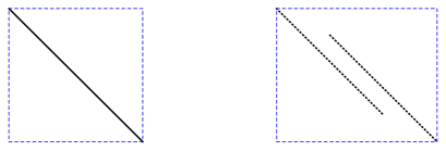
Figure 9. A deformation of $\Delta$ resulting in a disappearing tropical Lagrangian.

Note that in this example $\kappa=2$, $\mathfrak{z}_{1}=\mathfrak{z}_{2}=(1,0,0)$, so

$$(\mathfrak{z}_{1},\mathfrak{z}_{2})_{h}=(\mathfrak{z}_{1},\mathfrak{z}_{2},(dh)e)=0,$$

where $dh(e)=(1,-1,0)$ is the primitive integer vector parallel to the only edge of $C$.

Proof of Theorem 6.9.

Choose a bissectrice point $p\in C\cap\partial\Delta$ as the root of the tree $C$, and orient all edges of $C$ towards $p$. We adopt the notation $T_{e}$ from the proof of Lemma 2.3. We have $T_{e}=\{\iota(e)\}\times(y+\Theta_{e})$.

Let $L^{+}(e)\subset L$ be component of $L\smallsetminus T_{e}$ that is disjoint from $(\mu_{\Delta}\circ\nu_{\epsilon})^{-1}(p)$. We have $\partial L^{+}(e)=T_{e}\approx(S^{1})^{2}$ while

$$H_{1}(T_{e};\mathbb{R})\subset H_{1}((\mathbb{R}/2\pi\mathbb{Z})^{3};\mathbb{R})=\mathbb{R}^{3}$$

is a 2-plane conormal to the edge $e$. Denote $\operatorname{mv}(e)=\prod\limits_{v}m(v)$, where the product is taken over all vertices of $C$ that correspond to $L^{+}(e)$, i.e. all the vertices that precede $e$ in the order corresponding to the orientation given by the root vertex $p$.

Lemma 6.12.

If the rotational momentum $\rho(e)$ of an edge $e\in E_{C}$ is not zero then the torsion of $H_{1}(L^{+}(e))$ is a finite group of order $n(e)/\operatorname{mv}(e)$, where $n(e)$ is the GCD of the coordinates of $\rho(e)$, i.e. $\rho(e)=n(e)\rho^{\prime}(e)$ for a primitive vector $\rho^{\prime}(e)\in\mathbb{Z}^{3}$.

Furthermore, the bivector in $\Lambda^{2}(\mathbb{R}^{3})$ corresponding to $\rho(e)$ (see (18)) is conormal to the kernel of $H_{1}(T_{e};\mathbb{R})\to H_{1}(L^{+}(e);\mathbb{R})$.

Recall that the vector product of two vectors $u_{1},u_{2}\in\mathbb{R}^{3}$ may be defined (using the scalar product $(,)$ in $\mathbb{R}^{3}$) through the identity

(18) $$u_{1}\wedge u_{2}\wedge u=(u_{1}\times u_{2},u)\operatorname{vol}$$

that should hold for any vector $u\in\mathbb{R}^{3}$ for the volume 3-vector $\operatorname{vol}\in\Lambda^{3}(\mathbb{R}^{3})$ defined by the metric $(,)$. The vector product can be thought of just as a vector encoding of this bivector through (18) with the help of the scalar product in $\mathbb{R}^{3}$. Since by its definition the rotational momentum $\rho(e)$ is obtained as the vector product of a certain (inductively defined) vector and $u_{e}$, the vectors $\rho(e)$ and $u_{e}$ are not parallel unless $\rho(e)=0$.

Proof of Lemma 6.12.

Suppose that $e\subset C$ is a leaf not adjacent to the root vertex $p$. Then $e$ is adjacent to another bissectrice point $p_{e}\in C\cap\partial\Delta$. Let $\mathfrak{z}_{e}\in\mathbb{Z}^{3}$ be a primitive tangent vector to the edge of $\partial\Delta$ containing the point $p_{e}$. By the construction of $M_{\Delta}$, $L^{+}(e)\approx S^{1}\times D^{2}$ and the kernel of $H_{1}(T_{e};\mathbb{R})\to H_{1}(L^{+}(e);\mathbb{R})$ is cut by the conormal torus of $\mathfrak{z}_{e}$ (i.e. the torus conormal to the bivector encoded by $\rho(e)$ through (18)). In this case there is no torsion in $H_{1}(L^{+}(e);\mathbb{Z})\approx\mathbb{Z}$. Also $\rho(e)$ is primitive as $p_{e}$ is a bissectrice point.

Let $e$ be an oriented edge whose source is a 3-valent vertex $v\in V_{C}$. By the induction hypothesis we know that the lemma already holds for the two edges $\iota_{1},\iota_{2}$ that are incoming with respect to $v$. Suppose at first that $m(v)=1$. Then $\nu_{\epsilon}$ induces an isomorphism between $H_{1}(Q_{v})$ and $H_{1}(\mathbb{C}^{3})=H_{1}(\Theta)=\mathbb{Z}^{3}$ for the component $Q_{v}\approx P\times S^{1}$ of $L\smallsetminus T$ corresponding to $v$ (i.e. bounded by the tori $T_{\iota_{1}}$, $T_{\iota_{2}}$ and $T_{e}$). The kernel $K_{e}$ of $H_{1}(T_{e})\to H_{1}(L^{+}(e))$ is cut in $H_{1}(T_{e})\subset\mathbb{Z}^{3}$ by $K_{\iota_{1}}+K_{\iota_{2}}$ (which is two-dimensional by the induction hypothesis unless $\rho(e)=0$).

Let $\Lambda_{\iota}\subset\mathbb{Z}^{3}$ be the lattice formed by the integer vectors parallel to the elements of $K_{\iota_{1}}+K_{\iota_{2}}$. Consider the inclusion homomorphism

$$H_{1}(L^{+}(\iota_{1})\cup L^{+}(\iota_{2}))\to H_{1}(L^{+}(e))$$

from the exact sequence of the pair $(L^{+}(e),L^{+}(\iota_{1})\cup L^{+}(\iota_{2}))$. By the excision property, the homology groups to the left and to the right of this homomorphism in the long exact sequence are torsion-free. Thus the torsion of $H_{1}(L^{+}(e))$ decomposes into the sum of the torsions of $H_{1}(L^{+}(\iota_{j}))$, $j=1,2$, and the quotient $\Lambda_{\iota}/(K_{\iota_{1}}+K_{\iota_{2}})$. Thus $\#(H_{1}(L^{+}(e)))$ equals to $n(\iota_{1})n(\iota_{2})$ times the GCD of the coordinates of $\rho^{\prime}(\iota_{1})\times\rho^{\prime}(\iota_{2})$. The kernel $K_{e}\otimes\mathbb{R}$ is the intersection of $K_{\iota_{1}}\otimes\mathbb{R}+K_{\iota_{2}}\otimes\mathbb{R}$ with $H_{1}(T_{e};\mathbb{R})\subset H_{1}(\Theta;\mathbb{R})=\mathbb{R}^{3}$ and thus is conormal to the bivector corresponding to $\rho(\iota_{1})\times\rho(\iota_{2})$.

If $m(v)>1$ then the homomorphism $H_{1}(Q_{v})\to H_{1}(\mathbb{C}^{3})=\mathbb{Z}^{3}$ induced by $\nu_{\epsilon}$ is injective, but not surjective. Its image is a sublattice of index $m(v)$. Thus to get $\#(H_{1}(L^{+}(e)))$ we have to divide the product of $n(\iota_{1})n(\iota_{2})$ and the GCD of the coordinates of $\rho^{\prime}(\iota_{1})\times\rho^{\prime}(\iota_{2})$ by $m(v)$. The kernel of $H_{1}(T_{e};\mathbb{R})\to H_{1}(L^{+}(e);\mathbb{R})$ is defined over $\mathbb{R}$, thus its computation is the same as in the $m(v)=1$ case. ∎

To finish the proof of Theorem 6.9 we apply Lemma 6.12 to the leaf $e_{p}$ of $C$ adjacent to the bissectrice point $p$. The manifold $L$ is obtained by gluing of $L^{+}(e_{p})$ and $S^{1}\times D^{2}$ along their common boundary $T_{e}\approx(S^{1})^{2}$. The kernels of the maps from $H_{1}(T_{e})$ into these 3-folds are isomorphic to $\mathbb{Z}$ and described by the rotational momenta $\rho(e)$ and $\rho_{p}$. The cardinality $\#(H_{1}(L))$ equals to the product of the cardinality of the torsion subgroup of $H_{1}(L^{+}(e_{p}))$ and the GCD of the coordinates of $\rho^{\prime}(e)\times\rho_{p}$ (recall that $\rho_{p}$ is primitive as $p$ is a bissectrice point), i.e. to $(\mathfrak{z}_{1},\dots,\mathfrak{z}_{\kappa})_{h}$ in the case when the latter quantity is non-zero. If $(\mathfrak{z}_{1},\dots,\mathfrak{z}_{\kappa})_{h}=0$ then $H_{1}(L;\mathbb{R})\neq 0$. ∎

Remark 6.13.

Note that the topology of $L$ is determined by the tropical curve $C\subset L$ and the lines containing the edges of $\Delta$ incident to $C$. In other words, it is determined by the tropical curve $h:\Gamma\to\mathbb{R}^{3}$ and the lines $\mathfrak{L}$ forming a boundary configuration for $h$. Furthermore, we may construct the 3-manifold $L$ even in the case when no suitable Delzant domain for $(h,\mathfrak{L})$ exists.

Upgrading the tropical multiplicity $m(h,\mathfrak{L})$ to a torsion group $H_{1}(L)$ of order $m(h,\mathfrak{L})$ may be considered as a certain refinement of $m(h,\mathfrak{L})$. It might be interesting to attempt to extract finer invariants in tropical enumerative problems using $H_{1}(L)$, and perhaps even more interesting using other invariants of $\pi_{1}(L)$ or the graph 3-fold $L$ itself.

Definition 6.14.

Let $h:\Gamma\to\mathbb{R}^{3}$ be a primitive tropical immersion of a graph $\Gamma$ with $\kappa$ ends, and $\mathfrak{L}=(\mathfrak{l}_{1},\dots,\mathfrak{l}_{\kappa})$ be a generic boundary configuration of lines for $h$ parallel to $\mathcal{Z}=(\mathfrak{z}_{1},\dots,\mathfrak{z}_{\kappa})$. We say that a Delzant polyhedral domain $\Delta\subset\mathbb{R}^{3}$ is $(h,\mathfrak{L})$-suitable if for each $j=1,\dots,\kappa$ there exists an edge $e_{j}$ of $\Delta$ parallel to $\mathfrak{z}_{j}$ such that $e_{j}\supset h(\Gamma)\cap\mathfrak{l}_{j}$ and all points of $\partial\Delta\cap h(\Gamma)$ are bissectrice points.

Determining existence of a $(h,\mathfrak{L})$-suitable domain seems to be a non-trivial problem. Still it is easy to establish some necessary conditions. Let $\mathcal{D}=(d_{1},\dots,d_{\kappa})$ be the toric degree of $h$ and $p_{j}\in\mathfrak{l}_{j}$ be the points of intersection of the line $\mathfrak{l}_{j}$ and the leaf of $h(\Gamma)$ parallel to $d_{j}\in\mathbb{Z}^{3}$. Let $P$ be the convex hull of $\bigcup_{j=1}^{\kappa}\{p_{j}\}$.

Proposition 6.15.

If $\Delta\subset\mathbb{R}^{3}$ is an $(h,\mathfrak{L})$-suitable polyhedral domain for a generic configuration $\mathfrak{L}$ then $d_{j}\times\mathfrak{z}_{j}\in\mathbb{Z}^{3}$ is primitive and $p_{j}$ is a vertex of the polyhedron $P$ for every $j=1,\dots,\kappa$.

Proof.

Since an $(h,\mathfrak{L})$-suitable polyhedral domain $\Delta$ is convex and $p_{j}$ is contained in the 1-skeleton of $\partial\Delta$, the point $p_{j}$ must be contained in the 1-skeleton of $P$. If $p_{j}$ is not a vertex then it is contained in the interval between two other bissectrice points all sharing the same line from $\mathfrak{L}$. This contradicts to the assumption that $\mathfrak{L}$ is generic.

Since $p_{j}$ is a bissectrice point for an edge of the Delzant domain $\Delta$ parallel to $\mathfrak{z}_{j}$, the vector $d_{j}$ can be presented as the sum of two vectors $a_{j}$ and $b_{j}$ (parallel to the adjacent faces of $\Delta$) such that $a_{j},b_{j},\mathfrak{z}_{j}$ is a basis of $\mathbb{Z}^{3}$. Thus $d_{j}\times\mathfrak{z}_{j}$ is primitive. ∎

The first necessary condition given by Proposition 6.15 is also sufficient to present the compact 3-manifold $L$ corresponding to $h$ as a smooth Lagrangian manifold in a non-compact symplectic toric manifold corresponding to, perhaps, a non-convex domain $\Delta$ (but still convex and polyhedral near its boundary faces), cf. Remark 1.3.

Let $\mathfrak{L}$ be a generic boundary configuration for a primitive tropical curve $h:\Gamma\to\mathbb{R}^{3}$. Denote with $C\subset\mathbb{R}^{3}$ the closure of the the only bounded component of $h(\Gamma)\smallsetminus\bigcup\limits_{j=1}^{\kappa}(p_{j})$. Note that for any $(h,\mathfrak{L})$-suitable Delzant domain $\Delta$ we have $C=h(\Gamma)\cap\Delta$.

Proposition 6.16.

If $\mathfrak{L}$ is a generic boundary configuration for a primitive tropical immersion $h:\Gamma\to\mathbb{R}^{3}$, and $d_{j}\times\mathfrak{z}_{j}\in\mathbb{Z}^{3}$ is primitive for any $j=1,\dots,\kappa$ then there exists a set $\Delta\subset\mathbb{R}^{3}$ and its subset $\partial\Delta\subset\mathbb{R}^{3}$ such that the following conditions hold.

1. $\Delta\supset C$, $p_{j}\in\partial\Delta$, $j=1,\dots,\kappa$.

2. $\Delta$ is locally a Delzant polyhedral domain near any point of $\partial\Delta$ and $p_{j}$ is a bissectrice point so that $C$ is an even primitive tropical curve in $\Delta$.

3. The set $\Delta\smallsetminus\partial\Delta$ is open.

4. The curve $C\subset\Delta$ is Lagrangian-realizable in $M_{\Delta}$ in the sense of Definition 2.1.

Thus we may speak of a Lagrangian graph manifold $L$ for $(h,\mathfrak{L})$ even in the absence of an $(h,\mathfrak{L})$-suitable Delzant domain in $\mathbb{R}^{3}$.

Proof.

Since $d_{j}\times\mathfrak{z}_{j}$ is primitive, we may find $a_{j},b_{j}\in\mathbb{Z}^{3}$ such that $a_{j}+b_{j}=-d_{j}$, and $(a_{j},b_{j},\mathfrak{z}_{j})=1$, i.e. such that $a_{j},b_{j},\mathfrak{z}_{j}$ is a basis of $\mathbb{Z}^{3}$. Define $\Delta_{a_{j}}$ (resp. $\Delta_{b_{j}}$) to be the half-space passing through $p_{j}$ whose boundary is parallel to $\mathfrak{z}_{j}$ and $a_{j}$ (resp. $b_{j}$) and containing the edge of $C$ adjacent to $p_{j}$. The intersection $\Delta_{j}=\Delta_{a_{j}}\cap\Delta_{b_{j}}$ is a Delzant domain which has $\mathfrak{l}_{j}$ as its apex edge. We set

$$\Delta=U_{C}\cup\bigcup\limits_{j=1}^{\kappa}(U_{p_{j}}\cap\Delta_{j}),$$

where $U_{p_{j}}$ is a ball around $p_{j}$ of a small radius, and $U_{C}$ is a very small open neighborhood of $C$. The proof of Theorem 1 produces Lagrangian realizability of $C\subset\Delta$ in the (non-compact) symplectic manifold $M_{\Delta}$ in the same way as in the case when $\Delta$ is a global Delzant domain. ∎

The following two examples show that the topology of the Lagrangian 3-fold $L$ is not determined by the corresponding tropical multiplicity even in the case when the multiplicity is 1. In the first example we may find an $(h,\mathfrak{L})$-suitable Delzant domain $\Delta$. In the second example we do not claim existence of an $(h,\mathfrak{L})$-suitable Delzant domain, though we can still easily lift $L_{8}$ to a singular toric 3-fold $M_{\Delta}$ (for non-Delzant compact polyhedral domain $\Delta$) so that $L_{8}$ intersect the singular locus of $M_{\Delta}$. Also Proposition 6.16 provides a Lagrangian embedding of $L_{8}$ to a non-compact toric symplectic manifold.

Example 6.17 (Lens spaces).

Suppose that

$$C=[(0,0,0),(0,0,1)]\subset\mathbb{R}^{3}$$

is the interval , and $\Delta_{p,q}\supset C$ is a Delzant polyhedral domain such that it possesses edges contained in the line $\mathfrak{l}_{1}$ through $(0,0,0)$ parallel to the vector $\mathfrak{z}_{1}=(1,0,0)$ and in the line $\mathfrak{l}_{2}$ through $(0,0,1)$ parallel to the vector $\mathfrak{z}_{2}=(-q,p,0)$ for an integer $p>0$ and an integer $q$ relatively prime with $p$, and such that $(0,0,0)$ and $(0,0,1)$ are bissectrice points of $C$. Then Theorem 1 gives an embedded Lagrangian $L_{p,q}\subset M_{\Delta_{p,q}}$ diffeomorphic to the lens space $L(p,q)$. Note that the tropical multiplicity is $p$ while $L(p,q)$ and $L(p,q^{\prime})$ may be non-diffeomorphic.

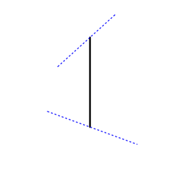
Figure 10. A Lagrangian lens space.

It is easy to see that such $\Delta_{p,q}$ exists for arbitrary $p,q$. Since $(0,0,1)\times\mathfrak{z}_{j}\in\mathbb{Z}^{3}$, $j=1,2$, is primitive, we may present $\mathfrak{l}_{j}$ as the apex edge of the intersection of two half-space such that $C$ has the boundary momentum 1 with respect to each of them. The intersection of the four half-space is a tetrahedron $\Delta^{\prime}_{p,q}$ which has rational slope, but is, perhaps, non-Delzant at some of its faces disjoint from $C$. To get $\Delta_{p,q}$ we truncate the tetrahedron $\Delta^{\prime}_{p,q}$ at such faces. Note that a truncation $\Delta_{p,q}\subset\Delta^{\prime}_{p,q}$ may be associated to a toric resolution $M_{\Delta_{p,q}}\to M_{\Delta^{\prime}_{p,q}}$ of the toric orbifold $M_{\Delta^{\prime}{p,q}}$.

Example 6.18 (The Poincaré sphere).

Let $e_{1}=[(-1,0,0),(0,0,0)]$, $e_{2}=[(0,-1,0),(0,0,0)]$, $e_{3}=[(0,0,0),(1,1,0)]$,

$$C=e_{1}\cup e_{2}\cup e_{3},$$

and $\mathfrak{l}_{j}$, $j=1,2,3$, be the lines passing through $p_{1}=(-1,0,0)$, $p_{2}=(0,-1,0)$, $p_{3}=(1,1,0)$, and parallel to $\mathfrak{z}_{1}=(0,1,2)$, $\mathfrak{z}_{2}=(1,0,3)$, $\mathfrak{z}_{3}=(0,1,5)$. The corresponding 3-manifold $L_{8}$ is obtained by gluing three solid tori to the product $P\times S^{1}$ of the pair-of-pants $P$ and the circle $S^{1}$ according to the rotational momenta of the leaves of $C$ which are $\rho_{1}=(0,2,-1)$, $\rho_{2}=(-3,0,1)$ and $\rho_{3}=(5,-5,1)$.

It is easy to see that $L_{8}$ is the Poincaré homology sphere, i.e. the Seifert-fibered homology sphere with three multiple fibers of Seifert invariant $(2,1)=(2,-1)$, $(3,1)$ and $(5,1)$, cf. [9].

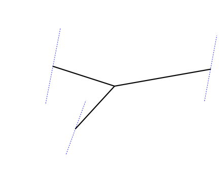
Figure 11. The Poincaré sphere from a tropical curve.

We may find a compact polyhedral domain $\Delta_{8}\supset C$ with edges parallel to $\mathfrak{z}_{j}$, containing $e_{j}$. A straightforward modification of Theorem 1 produces a Lagrangian mapping of $L_{8}$ to the orbifold $M_{\Delta_{8}}$.

To find $\Delta_{8}$ we define the convex domains $\Delta_{j}$, $j=1,2,3$, to be the convex hull of $\mathfrak{l}_{j}$ and the rays emanating from $p_{j}$ in the direction of $(1,1,0)$ and $(0,-1,0)$ for $j=1$; $(-1,0,0)$ and $(1,1,0)$ for $j=2$; $(0,-1,0)$ and $(-1,0,0)$ for $j=3$, see Figure 11. We set

$$\Delta_{8}=\{|x|\leq\epsilon\}\cup\bigcup_{j=1}^{3}\Delta_{j}$$

for a small $\epsilon>0$. It is a (non-Delzant) polyhedron with eight facets.

Perturbing $\Delta_{8}$ by introducing more faces to resolve singularities of $M_{\Delta_{8}}$ we may obtain a Delzant polyhedron $\tilde{\Delta}_{8}$ also containing $C$ in a way that the endpoints of $C$ sit on the edges of $\tilde{\Delta}_{8}$ parallel to $\mathfrak{l}_{j}$. This gives us a Lagrangian mapping of $L_{8}$ to the smooth symplectic toric manifold $M_{\tilde{\Delta}_{8}}$. Note, however, that this mapping is not an embedding unless the edges $e_{j}$ can be made bissectrices of the corresponding angles.

Question 6.19.

Does $L_{8}$ admit a Lagrangian embedding to a smooth symplectic toric manifold?

We have $m(h,\mathfrak{L})=1$ for the associated tropical problem both in Example 6.18 and in Example 6.17 for $p=1$. Nevertheless, topology of the corresponding Lagrangian manifolds is different: $L_{1,0}$ is the standard sphere $S^{3}$ while $L_{8}$ is the (non simply connected) Poincaré sphere.

Example 6.20.

Let $\Delta$ be the convex hull of $(0,0,0)$, $(1,0,0)$, $(0,1,0)$ and $(0,0,1)$. The baricenter of $\Delta$ is $p=(\frac{1}{4},\frac{1}{4},\frac{1}{4})$. Let

$$C_{12}=[(\frac{1}{4},0,0),p]\cup[(\frac{1}{2},\frac{1}{2},0),p]\cup[(0,\frac{1}{4},\frac{3}{4}),p].$$

It is easy to see that $C_{12}$ is a primitive tropical curve in $\Delta$ while the multiplicity of its only 3-valent vertex $p$ is 1. Thus there exists a Lagrangian embedding

$$L_{12}\subset M_{\Delta}={\mathbb{C}}{\mathbb{P}}^{3}$$

for a rational homology sphere $L_{12}$ with

$$\#(H_{1}(L_{12}))=|(\mathfrak{z}_{1},\mathfrak{z}_{2},\mathfrak{z}_{3})_{h}|=4,$$

where $\mathfrak{z}_{1}=(1,0,0)$, $\mathfrak{z}_{2}=(1,-1,0)$, $\mathfrak{z}_{3}=(0,1,-1)$ are primitive integer vectors in the directions parallel to the edges of $\Delta$ containing the endpoints of $C_{12}$.

It is interesting to compare the resulting $L_{12}$ against Chiang’s example of a nonstandard Lagrangian $L_{C}\subset{\mathbb{C}}{\mathbb{P}}^{3}$, see [4]. It is easy to see $\pi_{1}(L_{12})=\pi_{1}(L_{C})$ (in particular, that the fundamental group of $L_{12}$ has order 12).

Question 6.21.

Is $L_{12}$ Hamiltonian isotopic to Chiang’s Lagrangian submanifold $L_{C}\subset{\mathbb{C}}{\mathbb{P}}^{3}$?

Question 6.22.

Are there other rational homology 3-spheres (except for ${\mathbb{R}}{\mathbb{P}}^{3}$ and $L_{C}$) that admit Lagrangian embeddings to ${\mathbb{C}}{\mathbb{P}}^{3}$?

Note that according to Seidel’s theorem [19] we have $\#(H_{1}(L))\equiv 0\pmod{2}$ for any Lagrangian rational homology sphere $L\subset{\mathbb{C}}{\mathbb{P}}^{3}$.

Acknowledgment .

The author had benefited from many useful discussions with Tobias Ekholm, Yakov Eliashberg, Sergey Galkin, Alexander Givental, Ilia Itenberg, Conan Leung, Diego Matessi, Vivek Shende and Oleg Viro.

References

- [1] Ana Cannas da Silva. Lectures on symplectic geometry, volume 1764 of Lecture Notes in Mathematics. Springer-Verlag, Berlin, 2001.
- [2] Ana Cannas de Silva. A Chiang-type lagrangian in CP2. arXiv:1511.02041, to appear in Lett. Math. Phys.
- [3] Lucia Caporaso. Algebraic and tropical curves: comparing their moduli spaces. In Handbook of moduli. Vol. I, volume 24 of Adv. Lect. Math. (ALM), pages 119–160. Int. Press, Somerville, MA, 2013.
- [4] River Chiang. New Lagrangian submanifolds of . Int. Math. Res. Not., (45):2437–2441, 2004.
- [5] Thomas Delzant. Hamiltoniens périodiques et images convexes de l’application moment. Bull. Soc. Math. France, 116(3):315–339, 1988.
- [6] A. B. Givental′. Lagrangian imbeddings of surfaces and the open Whitney umbrella. Funktsional. Anal. i Prilozhen., 20(3):35–41, 96, 1986.
- [7] Nikita Kalinin and Grigory Mikhalkin. Tropical differential forms. In preparation.
- [8] Nikita Kalinin and Mikhail Shkolnikov. Tropical curves in sandpiles. C. R. Math. Acad. Sci. Paris, 354(2):125–130, 2016.
- [9] R. C. Kirby and M. G. Scharlemann. Eight faces of the Poincaré homology -sphere. Uspekhi Mat. Nauk, 37(5(227)):139–159, 1982. Translated from the English by S. N. Malygin.
- [10] Cheuk Yu Mak and Helge Ruddat. Tropically constructed lagrangians in mirror quintic threefolds. In preparation.
- [11] Travis Mandel and Helge Ruddat. Descendant log Gromov-Witten invariants for toric varieties and tropical curves. arXiv:1612.02402.
- [12] Travis Mandel and Helge Ruddat. Tropical quantum field theory, mirror polyvector fields, and multiplicities of tropical curves. In preparation.
- [13] Diego Matessi. Lagrangian pairs of pants. arXiv:1802.02993.
- [14] Grigory Mikhalkin. Enumerative tropical algebraic geometry in . J. Amer. Math. Soc., 18(2):313–377, 2005.
- [15] Grigory Mikhalkin. Tropical geometry and its applications. In International Congress of Mathematicians. Vol. II, pages 827–852. Eur. Math. Soc., Zürich, 2006.
- [16] Grigory Mikhalkin. Quantum indices and refined enumeration of real plane curves. Acta Math., 219:135–180, 2017.
- [17] Takeo Nishinou. Toric degenerations, tropical curve, and Gromov-Witten invariants of Fano manifolds. Canad. J. Math., 67(3):667–695, 2015.
- [18] Takeo Nishinou and Bernd Siebert. Toric degenerations of toric varieties and tropical curves. Duke Math. J., 135(1):1–51, 2006.
- [19] Paul Seidel. Graded Lagrangian submanifolds. Bull. Soc. Math. France, 128(1):103–149, 2000.
- [20] E. Shustin. A tropical approach to enumerative geometry. Algebra i Analiz, 17(2):170–214, 2005.
- [21] David E. Speyer. Parameterizing tropical curves I: Curves of genus zero and one. Algebra Number Theory, 8(4):963–998, 2014.
- [22] Ilya Tyomkin. Tropical geometry and correspondence theorems via toric stacks. Math. Ann., 353(3):945–995, 2012.
- [23] O. Ya. Viro. Real plane algebraic curves: constructions with controlled topology. Algebra i Analiz, 1(5):1–73, 1989.
- [24] Friedhelm Waldhausen. Eine Klasse von -dimensionalen Mannigfaltigkeiten. I, II. Invent. Math. 3 (1967), 308–333; ibid., 4:87–117, 1967.