Online convex optimization for cumulative constraints

Abstract

We propose the algorithms for online convex optimization which lead to cumulative squared constraint violations of the form $\sum\limits_{t=1}^{T}\big{(}[g(x_{t})]_{+}\big{)}^{2}=O(T^{1-\beta})$, where $\beta\in(0,1)$ . Previous literature has focused on long-term constraints of the form $\sum\limits_{t=1}^{T}g(x_{t})$. There, strictly feasible solutions can cancel out the effects of violated constraints. In contrast, the new form heavily penalizes large constraint violations and cancellation effects cannot occur. Furthermore, useful bounds on the single step constraint violation $[g(x_{t})]_{+}$ are derived. For convex objectives, our regret bounds generalize existing bounds, and for strongly convex objectives we give improved regret bounds. In numerical experiments, we show that our algorithm closely follows the constraint boundary leading to low cumulative violation.

1 Introduction

Online optimization is a popular framework for machine learning, with applications such as dictionary learning Mairal et al. (2009), auctions Blum et al. (2004), classification, and regression Crammer et al. (2006). It has also been influential in the development of algorithms in deep learning such as convolutional neural networks LeCun et al. (1998), deep Q-networks Mnih et al. (2015), and reinforcement learning Fazel et al. (2018); Yuan and Lamperski (2017).

The general formulation for online convex optimization (OCO) is as follows: At each time t, we choose a vector $x_{t}$ in convex set $S=\{x:g(x)\leq 0\}$. Then we receive a loss function $f_{t}:S\to R$ drawn from a family of convex functions and we obtain the loss $f_{t}(x_{t})$. In this general setting, there is no constraint on how the sequence of loss functions $f_{t}$ is generated. See Zinkevich (2003) for more details.

The goal is to generate a sequence of $x_{t}\in S$ for $t=1,2,..,T$ to minimize the cumulative regret which is defined by:

$$Regret_{T}(x^{*})=\sum\limits_{t=1}^{T}f_{t}(x_{t})-\sum\limits_{t=1}^{T}f_{t}(x^{*})$$ (1)

where $x^{*}$ is the optimal solution to the following problem: $\min\limits_{x\in S}\sum\limits_{t=1}^{T}f_{t}(x)$. According to Cesa-Bianchi and Lugosi (2006), the solution to Problem (1) is called Hannan consistent if $Regret_{T}(x^{*})$ is sublinear in $T$.

For online convex optimization with constraints, a projection operator is typically applied to the updated variables in order to make them feasible at each time step Zinkevich (2003); Duchi et al. (2008, 2010). However, when the constraints are complex, the computational burden of the projection may be too high for online computation. To circumvent this dilemma, Mahdavi et al. (2012) proposed an algorithm which approximates the true desired projection with a simpler closed-form projection. The algorithm gives a cumulative regret $Regret_{T}(x^{*})$ which is upper bounded by $O(\sqrt{T})$, but the constraint $g(x_{t})\leq 0$ may not be satisfied in every time step. Instead, the long-term constraint violation satisfies $\sum\limits_{t=1}^{T}g(x_{t})\leq O(T^{3/4})$, which is useful when we only require the constraint violation to be non-positive on average: $\lim_{T\to\infty}\sum\limits_{t=1}^{T}g(x_{t})/T\leq 0$.

More recently, Jenatton et al. (2016) proposed an adaptive stepsize version of this algorithm which can make $Regret_{T}(x^{*})\leq O(T^{\max\{\beta,1-\beta\}})$ and $\sum\limits_{t=1}^{T}g(x_{t})\leq O(T^{1-\beta/2})$. Here $\beta\in(0,1)$ is a user-determined trade-off parameter. In related work, Yu et al. (2017) provides another algorithm which achieves $O(\sqrt{T})$ regret and a bound of $O(\sqrt{T})$ on the long-term constraint violation.

In this paper, we propose two algorithms for the following two different cases:

Convex Case: The first algorithm is for the convex case, which also has the user-determined trade-off as in Jenatton et al. (2016), while the constraint violation is more strict. Specifically, we have $Regret_{T}(x^{*})\leq O(T^{\max\{\beta,1-\beta\}})$ and $\sum\limits_{t=1}^{T}\big{(}[g(x_{t})]_{+}\big{)}^{2}\leq O(T^{1-\beta})$ where $[g(x_{t})]_{+}=\max\{0,g(x_{t})\}$ and $\beta\in(0,1)$. Note the square term heavily penalizes large constraint violations and constraint violations from one step cannot be canceled out by strictly feasible steps. Additionally, we give a bound on the cumulative constraint violation $\sum\limits_{t=1}^{T}[g(x_{t})]_{+}\leq O(T^{1-\beta/2})$, which generalizes the bounds from Mahdavi et al. (2012); Jenatton et al. (2016).

In the case of $\beta=0.5$, which we call "balanced", both $Regret_{T}(x^{*})$ and $\sum\limits_{t=1}^{T}([g(x_{t})]_{+})^{2}$ have the same upper bound of $O(\sqrt{T})$. More importantly, our algorithm guarantees that at each time step, the clipped constraint term $[g(x_{t})]_{+}$ is upper bounded by $O(\frac{1}{T^{1/6}})$, which does not follow from the results of Mahdavi et al. (2012); Jenatton et al. (2016). However, our results currently cannot generalize those of Yu et al. (2017), which has $\sum\limits_{t=1}^{T}g(x_{t})\leq O(\sqrt{T})$. As discussed below, it is unclear how to extend the work of Yu et al. (2017) to the clipped constraints, $[g(x_{t})]_{+}$.

Strongly Convex Case: Our second algorithm for strongly convex function $f_{t}(x)$ gives us the improved upper bounds compared with the previous work in Jenatton et al. (2016). Specifically, we have $Regret_{T}(x^{*})\leq O(\log(T))$, and $\sum\limits_{t=1}^{T}[g(x_{t})]_{+}\leq O(\sqrt{\log(T)T})$. The improved bounds match the regret order of standard OCO from Hazan et al. (2007), while maintaining a constraint violation of reasonable order.

We show numerical experiments on three problems. A toy example is used to compare trajectories of our algorithm with those of Jenatton et al. (2016); Mahdavi et al. (2012), and we see that our algorithm tightly follows the constraints. The algorithms are also compared on a doubly-stochastic matrix approximation problem Jenatton et al. (2016) and an economic dispatch problem from power systems. In these, our algorithms lead to reasonable objective regret and low cumulative constraint violation.

2 Problem Formulation

The basic projected gradient algorithm for Problem (1) was defined in Zinkevich (2003). At each step, $t$, the algorithm takes a gradient step with respect to $f_{t}$ and then projects onto the feasible set. With some assumptions on $S$ and $f_{t}$, this algorithm achieves a regret of $O(\sqrt{T})$.

Although the algorithm is simple, it needs to solve a constrained optimization problem at every time step, which might be too time-consuming for online implementation when the constraints are complex. Specifically, in Zinkevich (2003), at each iteration $t$, the update rule is:

$$\begin{array}[]{lll}x_{t+1}&=\Pi_{S}(x_{t}-\eta\nabla f_{t}(x_{t}))&=\arg\min\limits_{y\in S}\left\|y-(x_{t}-\eta\nabla f_{t}(x_{t}))\right\|^{2}\end{array}$$ (2)

where $\Pi_{S}$ is the projection operation to the set $S$ and $\left\|\quad\right\|$ is the $\ell_{2}$ norm.

In order to lower the computational complexity and accelerate the online processing speed, the work of Mahdavi et al. (2012) avoids the convex optimization by projecting the variable to a fixed ball $S\subseteq\mathcal{B}$, which always has a closed-form solution. That paper gives an online solution for the following problem:

$$\begin{array}[]{llll}\underset{x_{1},\ldots,x_{T}\in\mathcal{B}}{\min}&\sum\limits_{t=1}^{T}f_{t}(x_{t})-\min\limits_{x\in S}\sum\limits_{t=1}^{T}f_{t}(x)&s.t.&\sum\limits_{t=1}^{T}g_{i}(x_{t})\leq 0,i=1,2,...,m\end{array}$$ (3)

where $S=\{x:g_{i}(x)\leq 0,i=1,2,...,m\}\subseteq\mathcal{B}$. It is assumed that there exist constants $R>0$ and $r<1$ such that $r\mathbb{K}\subseteq S\subseteq R\mathbb{K}$ with $\mathbb{K}$ being the unit $\ell_{2}$ ball centered at the origin and $\mathcal{B}=R\mathbb{K}$.

Compared to Problem (1), which requires that $x_{t}\in S$ for all $t$, (3) implies that only the sum of constraints is required. This sum of constraints is known as the long-term constraint.

To solve this new problem, Mahdavi et al. (2012) considers the following augmented Lagrangian function at each iteration $t$:

$$\mathcal{L}_{t}(x,\lambda)=f_{t}(x)+\sum\limits_{i=1}^{m}\Big{\{}\lambda_{i}g_{i}(x)-\frac{\sigma\eta}{2}\lambda_{i}^{2}\Big{\}}$$ (4)

The update rule is as follows:

$$\begin{array}[]{ll}x_{t+1}=\Pi_{\mathcal{B}}(x_{t}-\eta\nabla_{x}\mathcal{L}_{t}(x_{t},\lambda_{t})),&\lambda_{t+1}=\Pi_{[0,+\infty)^{m}}(\lambda_{t}+\eta\nabla_{\lambda}\mathcal{L}_{t}(x_{t},\lambda_{t}))\end{array}$$ (5)

where $\eta$ and $\sigma$ are the pre-determined stepsize and some constant, respectively.

More recently, an adaptive version was developed in Jenatton et al. (2016), which has a user-defined trade-off parameter. The algorithm proposed by Jenatton et al. (2016) utilizes two different stepsize sequences to update $x$ and $\lambda$, respectively, instead of using a single stepsize $\eta$.

In both algorithms of Mahdavi et al. (2012) and Jenatton et al. (2016), the bound for the violation of the long-term constraint is that $\forall i$, $\sum\limits_{t=1}^{T}g_{i}(x_{t})\leq O(T^{\gamma})$ for some $\gamma\in(0,1)$. However, as argued in the last section, this bound does not enforce that the violation of the constraint $x_{t}\in S$ gets small. A situation can arise in which strictly satisfied constraints at one time step can cancel out violations of the constraints at other time steps. This problem can be rectified by considering clipped constraint, $[g_{i}(x_{t})]_{+}$, in place of $g_{i}(x_{t})$.

For convex problems, our goal is to bound the term $\sum\limits_{t=1}^{T}\big{(}[g_{i}(x_{t})]_{+}\big{)}^{2}$, which, as discussed in the previous section, is more useful for enforcing small constraint violations, and also recovers the existing bounds for both $\sum\limits_{t=1}^{T}[g_{i}(x_{t})]_{+}$ and $\sum\limits_{t=1}^{T}g_{i}(x_{t})$. For strongly convex problems, we also show the improvement on the upper bounds compared to the results in Jenatton et al. (2016).

In sum, in this paper, we want to solve the following problem for the general convex condition:

$$\begin{array}[]{llll}\min\limits_{x_{1},x_{2},...,x_{T}\in\mathcal{B}}&\sum\limits_{t=1}^{T}f_{t}(x_{t})-\min\limits_{x\in S}\sum\limits_{t=1}^{T}f_{t}(x)&\quad\quad s.t.&\sum\limits_{t=1}^{T}\big{(}[g_{i}(x_{t})]_{+}\big{)}^{2}\leq O(T^{\gamma}),\forall i\end{array}$$ (6)

where $\gamma\in(0,1)$. The new constraint from (6) is called the square-clipped long-term constraint (since it is a square-clipped version of the long-term constraint) or square-cumulative constraint (since it encodes the square-cumulative violation of the constraints).

To solve Problem (6), we change the augmented Lagrangian function $\mathcal{L}_{t}$ as follows:

$$\mathcal{L}_{t}(x,\lambda)=f_{t}(x)+\sum\limits_{i=1}^{m}\Big{\{}\lambda_{i}[g_{i}(x)]_{+}-\frac{\theta_{t}}{2}\lambda_{i}^{2}\Big{\}}$$ (7)

In this paper, we will use the following assumptions as in Mahdavi et al. (2012): 1. The convex set $S$ is non-empty, closed, bounded, and can be described by $m$ convex functions as $S=\{x:g_{i}(x)\leq 0,i=1,2,...,m\}$. 2. Both the loss functions $f_{t}(x)$, $\forall t$ and constraint functions $g_{i}(x)$, $\forall i$ are Lipschitz continuous in the set $\mathcal{B}$. That is, $\left\|f_{t}(x)-f_{t}(y)\right\|\leq L_{f}\left\|x-y\right\|$, $\left\|g_{i}(x)-g_{i}(y)\right\|\leq L_{g}\left\|x-y\right\|$, $\forall x,y\in\mathcal{B}$ and $\forall t,i$. $G=\max\{L_{f},L_{g}\}$, and

$$\begin{array}[]{ll}F=\max\limits_{t=1,2,...,T}\max\limits_{x,y\in\mathcal{B}}f_{t}(x)-f_{t}(y)\leq 2L_{f}R,&D=\max\limits_{i=1,2,...,m}\max\limits_{x\in\mathcal{B}}g_{i}(x)\leq L_{g}R\end{array}$$

3 Algorithm

3.1 Convex Case:

Algorithm 1 Generalized Online Convex Optimization with Long-term Constraint

1:  Input: constraints $g_{i}(x)\leq 0,i=1,2,...,m$, stepsize $\eta$, time horizon T, and constant $\sigma>0$.

2:  Initialization: $x_{1}$ is in the center of the $\mathcal{B}$ .

3:  for $t=1$ to $T$ do

4:     Input the prediction result $x_{t}$.

5:     Obtain the convex loss function $f_{t}(x)$ and the loss value $f_{t}(x_{t})$.

6:     Calculate a subgradient $\partial_{x}\mathcal{L}_{t}(x_{t},\lambda_{t})$, where:

$$\begin{array}[]{ll}\partial_{x}\mathcal{L}_{t}(x_{t},\lambda_{t})=\partial_{x}f_{t}(x_{t})+\sum\limits_{i=1}^{m}\lambda_{t}^{i}\partial_{x}([g_{i}(x_{t})]_{+}),&\partial_{x}([g_{i}(x_{t})]_{+})=\begin{cases}0,\quad\mbox{$g_{i}(x_{t})\leq 0$}\\ \nabla_{x}g_{i}(x_{t}),\mbox{otherwise}\\ \end{cases}\end{array}$$

7:     Update $x_{t}$ and $\lambda_{t}$ as below:

$$\begin{array}[]{ll}x_{t+1}=\Pi_{\mathcal{B}}(x_{t}-\eta\partial_{x}\mathcal{L}_{t}(x_{t},\lambda_{t})),\lambda_{t+1}=\frac{[g(x_{t+1})]_{+}}{\sigma\eta}\end{array}$$

8:  end for

The main algorithm for this paper is shown in Algorithm 1. For simplicity, we abuse the subgradient notation, denoting a single element of the subgradient by $\partial_{x}\mathcal{L}_{t}(x_{t},\lambda_{t})$. Comparing our algorithm with Eq.(5), we can see that the gradient projection step for $x_{t+1}$ is similar, while the update rule for $\lambda_{t+1}$ is different. Instead of a projected gradient step, we explicitly maximize $\mathcal{L}_{t+1}(x_{t+1},\lambda)$ over $\lambda$. This explicit projection-free update for $\lambda_{t+1}$ is possible because the constraint clipping guarantees that the maximizer is non-negative. Furthermore, this constraint-violation-dependent update helps to enforce small cumulative and individual constraint violations. Specific bounds on constraint violation are given in Theorem 1 and Lemma 1 below.

Based on the update rule in Algorithm 1, the following theorem gives the upper bounds for both the regret on the loss and the squared-cumulative constraint violation, $\sum\limits_{t=1}^{T}\Big{(}[g_{i}(x_{t})]_{+}\Big{)}^{2}$ in Problem 6. For space purposes, all proofs are contained in the supplementary material.

Theorem 1.

Set $\sigma=\frac{(m+1)G^{2}}{2(1-\alpha)}$, $\eta=\frac{1}{G\sqrt{(m+1)RT}}$. If we follow the update rule in Algorithm 1 with $\alpha\in(0,1)$ and $x^{*}$ being the optimal solution for $\min\limits_{x\in S}\sum\limits_{t=1}^{T}f_{t}(x)$, we have

$$\begin{array}[]{ll}\sum\limits_{t=1}^{T}\Big{(}f_{t}(x_{t})-f_{t}(x^{*})\Big{)}\leq O(\sqrt{T}),&\sum\limits_{t=1}^{T}\Big{(}[g_{i}(x_{t})]_{+}\Big{)}^{2}\leq O(\sqrt{T}),\forall i\in\{1,2,...,m\}\end{array}$$

From Theorem 1, we can see that by setting appropriate stepsize, $\eta$, and constant, $\sigma$, we can obtain the upper bound for the regret of the loss function being less than or equal to $O(\sqrt{T})$, which is also shown in Mahdavi et al. (2012) Jenatton et al. (2016). The main difference of the Theorem 1 is that previous results of Mahdavi et al. (2012) Jenatton et al. (2016) all obtain the upper bound for the long-term constraint $\sum\limits_{t=1}^{T}g_{i}(x_{t})$, while here the upper bound for the constraint violation of the form $\sum\limits_{t=1}^{T}\Big{(}[g_{i}(x_{t})]_{+}\Big{)}^{2}$ is achieved. Also note that the stepsize depends on $T$, which may not be available. In this case, we can use the ’doubling trick’ described in the book Cesa-Bianchi and Lugosi (2006) to transfer our $T$-dependent algorithm into $T$-free one with a worsening factor of $\sqrt{2}/(\sqrt{2}-1)$.

The proposed algorithm and the resulting bound are useful for two reasons: 1. The square-cumulative constraint implies a bound on the cumulative constraint violation, $\sum\limits_{t=1}^{T}[g_{i}(x_{t})]_{+}$, while enforcing larger penalties for large violations. 2. The proposed algorithm can also upper bound the constraint violation for each single step $[g_{i}(x_{t})]_{+}$, which is not bounded in the previous literature.

The next results show how to bound constraint violations at each step.

Lemma 1.

If there is only one differentiable constraint function $g(x)$ with Lipschitz continuous gradient parameter $L$, and we run the Algorithm 1 with the parameters in Theorem 1 and large enough $T$, we have

$$\begin{array}[]{lll}[g(x_{t})]_{+}\leq O(\frac{1}{T^{1/6}}),&\forall t\in\{1,2,...,T\},&if\quad[g(x_{1})]_{+}\leq O(\frac{1}{T^{1/6}}).\end{array}$$

Lemma 1 only considers single constraint case. For case of multiple differentiable constraints, we have the following:

Proposition 1.

For multiple differentiable constraint functions $g_{i}(x)$, $i\in\{1,2,...,m\}$ with Lipschitz continuous gradient parameters $L_{i}$, if we use $\bar{g}(x)=\log\Big{(}\sum\limits_{i=1}^{m}\exp{g_{i}(x)}\Big{)}$ as the constraint function in Algorithm 1, then for large enough $T$, we have

$$\begin{array}[]{lll}[g_{i}(x_{t})]_{+}\leq O(\frac{1}{T^{1/6}}),&\forall i,t,&if\quad[\bar{g}(x_{1})]_{+}\leq O(\frac{1}{T^{1/6}}).\end{array}$$

Clearly, both Lemma 1 and Proposition 1 only deal with differentiable functions. For a non-differentiable function $g(x)$, we can first use a differentiable function $\bar{g}(x)$ to approximate the $g(x)$ with $\bar{g}(x)\geq g(x)$, and then apply the previous Lemma 1 and Proposition 1 to upper bound each individual $g_{i}(x_{t})$. Many non-smooth convex functions can be approximated in this way as shown in Nesterov (2005).

3.2 Strongly Convex Case:

For $f_{t}(x)$ to be strongly convex, the Algorithm 1 is still valid. But in order to have lower upper bounds for both objective regret and the clipped long-term constraint $\sum\limits_{t=1}^{T}[g_{i}(x_{t})]_{+}$ compared with Proposition 3 in next section, we need to use time-varying stepsize as the one used in Hazan et al. (2007). Thus, we modify the update rule of $x_{t}$, $\lambda_{t}$ to have time-varying stepsize as below:

$$\begin{array}[]{ll}x_{t+1}=\Pi_{\mathcal{B}}(x_{t}-\eta_{t}\partial_{x}\mathcal{L}_{t}(x_{t},\lambda_{t})),&\lambda_{t+1}=\frac{[g(x_{t+1})]_{+}}{\theta_{t+1}}.\end{array}$$ (8)

If we replace the update rule in Algorithm 1 with Eq.(8), we can obtain the following theorem:

Theorem 2.

Assume $f_{t}(x)$ has strongly convexity parameter $H_{1}$. If we set $\eta_{t}=\frac{1}{H_{1}(t+1)}$, $\theta_{t}=\eta_{t}(m+1)G^{2}$, follow the new update rule in Eq.(8), and $x^{*}$ being the optimal solution for $\min\limits_{x\in S}\sum\limits_{t=1}^{T}f_{t}(x)$, for $\forall i\in\{1,2,...,m\}$, we have

$$\begin{array}[]{ll}\sum\limits_{t=1}^{T}\Big{(}f_{t}(x_{t})-f_{t}(x^{*})\Big{)}\leq O(\log(T)),&\sum\limits_{t=1}^{T}g_{i}(x_{t})\leq\sum\limits_{t=1}^{T}[g_{i}(x_{t})]_{+}\leq O(\sqrt{\log(T)T}).\end{array}$$

The paper Jenatton et al. (2016) also has a discussion of strongly convex functions, but only provides a bound similar to the convex one. Theorem 2 shows the improved bounds for both objective regret and the constraint violation. On one hand the objective regret is consistent with the standard OCO result in Hazan et al. (2007), and on the other the constraint violation is further reduced compared with the result in Jenatton et al. (2016).

4 Relation with Previous Results

In this section, we extend Theorem 1 to enable direct comparison with the results from Mahdavi et al. (2012) Jenatton et al. (2016). In particular, it is shown how Algorithm 1 recovers the existing regret bounds, while the use of the new augmented Lagrangian (7) in the previous algorithms also provides regret bounds for the clipped constraint case.

The first result puts a bound on the clipped long-term constraint, rather than the sum-of-squares that appears in Theorem 1. This will allow more direct comparisons with the existing results.

Proposition 2.

If $\sigma=\frac{(m+1)G^{2}}{2(1-\alpha)}$, $\eta=O(\frac{1}{\sqrt{T}})$, $\alpha\in(0,1)$, and $x^{*}=\underset{x\in S}{\operatornamewithlimits{argmin}}\sum\limits_{t=1}^{T}f_{t}(x)$, then the result of Algorithm 1 satisfies

$$\begin{array}[]{ll}\sum\limits_{t=1}^{T}\Big{(}f_{t}(x_{t})-f_{t}(x^{*})\Big{)}\leq O(\sqrt{T}),&\sum\limits_{t=1}^{T}g_{i}(x_{t})\leq\sum\limits_{t=1}^{T}[g_{i}(x_{t})]_{+}\leq O(T^{3/4}),\forall i\in\{1,2,...,m\}\end{array}$$

This result shows that our algorithm generalizes the regret and long-term constraint bounds of Mahdavi et al. (2012).

The next result shows that by changing our constant stepsize accordingly, with the Algorithm 1, we can achieve the user-defined trade-off from Jenatton et al. (2016). Furthermore, we also include the squared version and clipped constraint violations.

Proposition 3.

If $\sigma=\frac{(m+1)G^{2}}{2(1-\alpha)}$, $\eta=O(\frac{1}{T^{\beta}})$, $\alpha\in(0,1)$, $\beta\in(0,1)$, and $x^{*}=\underset{x\in S}{\operatornamewithlimits{argmin}}\sum\limits_{t=1}^{T}f_{t}(x)$, then the result of Algorithm 1 satisfies

$$\begin{array}[]{lll}\sum\limits_{t=1}^{T}\Big{(}f_{t}(x_{t})-f_{t}(x^{*})\Big{)}\leq O(T^{max\{\beta,1-\beta\}}),\\ \sum\limits_{t=1}^{T}g_{i}(x_{t})\leq\sum\limits_{t=1}^{T}[g_{i}(x_{t})]_{+}\leq O(T^{1-\beta/2}),&\sum\limits_{t=1}^{T}([g_{i}(x_{t})]_{+})^{2}\leq O(T^{1-\beta}),\forall i\in\{1,2,...,m\}\end{array}$$

Proposition 3 provides a systematic way to balance the regret of the objective and the constraint violation. Next, we will show that previous algorithms can use our proposed augmented Lagrangian function to have their own clipped long-term constraint bound.

Proposition 4.

If we run Algorithm 1 in Mahdavi et al. (2012) with the augmented Lagrangian formula defined in Eq.(7), the result satisfies

$$\begin{array}[]{ll}\sum\limits_{t=1}^{T}\Big{(}f_{t}(x_{t})-f_{t}(x^{*})\Big{)}\leq O(\sqrt{T}),&\sum\limits_{t=1}^{T}g_{i}(x_{t})\leq\sum\limits_{t=1}^{T}[g_{i}(x_{t})]_{+}\leq O(T^{3/4}),\forall i\in\{1,2,...,m\}.\end{array}$$

For the update rule proposed in Jenatton et al. (2016), we need to change the $\mathcal{L}_{t}(x,\lambda)$ to the following one:

$$\mathcal{L}_{t}(x,\lambda)=f_{t}(x)+\lambda[g(x)]_{+}-\frac{\theta_{t}}{2}\lambda^{2}$$ (9)

where $g(x)=\max_{i\in\{1,\dots,m\}}g_{i}(x)$.

Proposition 5.

If we use the update rule and the parameter choices in Jenatton et al. (2016) with the augmented Lagrangian in Eq.(9), then $\forall i\in\{1,...,m\}$, we have

$$\begin{array}[]{ll}\sum\limits_{t=1}^{T}\Big{(}f_{t}(x_{t})-f_{t}(x^{*})\Big{)}\leq O(T^{max\{\beta,1-\beta\}}),&\sum\limits_{t=1}^{T}g_{i}(x_{t})\leq\sum\limits_{t=1}^{T}[g_{i}(x_{t})]_{+}\leq O(T^{1-\beta/2}).\end{array}$$

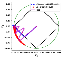
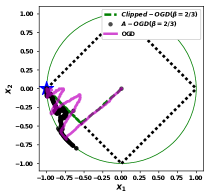
Figure 1: Toy Example Results: Trajectories generated by different algorithms. Note how trajectories generated by Clipped-OGD follow the desired constraints tightly. In contrast, OGD oscillates around the true constraints, and A-OGD closely follows the boundary of the outer ball.

Propositions 4 and 5 show that clipped long-term constraints can be bounded by combining the algorithms of Mahdavi et al. (2012); Jenatton et al. (2016) with our augmented Lagrangian. Although these results are similar in part to our Propositions 2 and 3, they do not imply the results in Theorems 1 and 2 as well as the new single step constraint violation bound in Lemma 1, which are our key contributions. Based on Propositions 4 and 5, it is natural to ask whether we could apply our new augmented Lagrangian formula (7) to the recent work in Yu et al. (2017) . Unfortunately, we have not found a way to do so.

Furthermore, since $\Big{(}[g_{i}(x_{t})]_{+}\Big{)}^{2}$ is also convex, we could define $\tilde{g}_{i}(x_{t})=\Big{(}[g_{i}(x_{t})]_{+}\Big{)}^{2}$ and apply the previous algorithms Mahdavi et al. (2012) Jenatton et al. (2016) and Yu et al. (2017). This will result in the upper bounds of $O(T^{3/4})$ Mahdavi et al. (2012) and $O(T^{1-\beta/2})$ Jenatton et al. (2016), which are worse than our upper bounds of $O(T^{1/2})$ (Theorem 1) and $O(T^{1-\beta})$ ( Proposition 3). Note that the algorithm in Yu et al. (2017) cannot be applied since the clipped constraints do not satisfy the required Slater condition.

5 Experiments

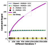
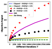
Figure 2: Doubly-Stochastic Matrices. Fig.2: Clipped Long-term Constraint Violation. Fig.2: Long-term Constraint Violation. Fig.2: Cumulative Regret of the Loss function

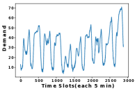
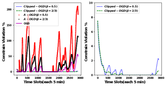
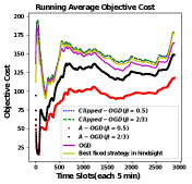
Figure 3: Economic Dispatch. Fig.3: Power Demand Trajectory. Fig.3: Constraint Violation for each time step. All of the previous algorithms incurred substantial constraint violations. The figure on the right shows the violations of our algorithm, which are significantly smaller. Fig.3: Running Average of the Objective Loss

In this section, we test the performance of the algorithms including OGD Mahdavi et al. (2012), A-OGD Jenatton et al. (2016), Clipped-OGD (this paper), and our proposed algorithm strongly convex case (Our-strong). Throughout the experiments, our algorithm has the following fixed parameters: $\alpha=0.5$, $\sigma=\frac{(m+1)G^{2}}{2(1-\alpha)}$, $\eta=\frac{1}{T^{\beta}G\sqrt{R(m+1)}}$. In order to better show the result of the constraint violation trajectories, we aggregate all the constraints as a single one by using $g(x_{t})=\max_{i\in\{1,...,m\}}g_{i}(x_{t})$ as done in Mahdavi et al. (2012).

5.1 A Toy Experiment

For illustration purposes, we solve the following 2-D toy experiment with $x=[x_{1},x_{2}]^{T}$:

$$\begin{array}[]{ll}\min\sum\limits_{t=1}^{T}c_{t}^{T}x,&s.t.\left|x_{1}\right|+\left|x_{2}\right|-1\leq 0.\end{array}$$ (10)

where the constraint is the $\ell_{1}$-norm constraint. The vector $c_{t}$ is generated from a uniform random vector over $[0,1.2]\times[0,1]$ which is rescaled to have norm $1$. This leads to slightly average cost on the on the first coordinate. The offline solutions for different $T$ are obtained by CVXPY Diamond and Boyd (2016).

All algorithms are run up to $T=20000$ and are averaged over 10 random sequences of $\{c_{t}\}_{t=1}^{T}$. Since the main goal here is to compare the variables’ trajectories generated by different algorithms, the results for different $T$ are in the supplementary material for space purposes. Fig.1 shows these trajectories for one realization with $T=8000$. The blue star is the optimal point’s position.

From Fig.1 we can see that the trajectories generated by Clipped-OGD follows the boundary very tightly until reaching the optimal point. This can be explained by the Lemma 1 which shows that the constraint violation for single step is also upper bounded. For the OGD, the trajectory oscillates widely around the boundary of the true constraint. For the A-OGD, its trajectory in Fig.1 violates the constraint most of the time, and this violation actually contributes to the lower objective regret shown in the supplementary material.

5.2 Doubly-Stochastic Matrices

We also test the algorithms for approximation by doubly-stochastic matrices, as in Jenatton et al. (2016):

$$\begin{array}[]{llll}\min\sum\limits_{t=1}^{T}\frac{1}{2}\left\|Y_{t}-X\right\|_{F}^{2}&s.t.\quad X\textbf{1}=\textbf{1},&X^{T}\textbf{1}=\textbf{1},&X_{ij}\geq 0.\end{array}$$ (11)

where $X\in\mathbb{R}^{d\times d}$ is the matrix variable, 1 is the vector whose elements are all 1, and matrix $Y_{t}$ is the permutation matrix which is randomly generated.

After changing the equality constraints into inequality ones (e.g.,$X\textbf{1}=\textbf{1}$ into $X\textbf{1}\geq\textbf{1}$ and $X\textbf{1}\leq\textbf{1}$), we run the algorithms with different T up to $T=20000$ for 10 different random sequences of $\{Y_{t}\}_{t=1}^{T}$. Since the objective function $f_{t}(x)$ is strongly convex with parameter $H_{1}=1$, we also include our designed strongly convex algorithm as another comparison. The offline optimal solutions are obtained by CVXPY Diamond and Boyd (2016).

The mean results for both constraint violation and objective regret are shown in Fig.2. From the result we can see that, for our designed strongly convex algorithm Our-Strong, its result is around the best ones in not only the clipped constraint violation, but the objective regret. For our most-balanced convex case algorithm Clipped-OGD with $\beta=0.5$, although its clipped constraint violation is relatively bigger than A-OGD, it also becomes quite flat quickly, which means the algorithm quickly converges to a feasible solution.

5.3 Economic Dispatch in Power Systems

This example is adapted from Li et al. (2018) and Senthil and Manikandan (2010), which considers the problem of power dispatch. That is, at each time step $t$, we try to minimize the power generation cost $c_{i}(x_{t,i})$ for each generator $i$ while maintaining the power balance $\sum\limits_{i=1}^{n}x_{t,i}=d_{t}$, where $d_{t}$ is the power demand at time $t$. Also, each power generator produces an emission level $E_{i}(x_{t,i})$. To bound the emissions, we impose the constraint $\sum\limits_{i=1}^{n}E_{i}(x_{t,i})\leq E_{max}$. In addition to requiring this constraint to be satisfied on average, we also require bounded constraint violations at each timestep. The problem is formally stated as:

$$\begin{array}[]{lll}\min\sum\limits_{t=1}^{T}\Big{(}\sum\limits_{i=1}^{n}c_{i}(x_{t,i})+\xi(\sum\limits_{i=1}^{n}x_{t,i}-d_{t})^{2}\Big{)},&s.t.\quad\sum\limits_{i=1}^{n}E_{i}(t,i)\leq E_{max},&0\leq x_{t,i}\leq x_{i,max}.\end{array}$$ (12)

where the second constraint is from the fact that each generator has the power generation limit.

In this example, we use three generators. We define the cost and emission functions according to Senthil and Manikandan (2010) and Li et al. (2018) as $c_{i}(x_{t,i})=0.5a_{i}x_{t,i}^{2}+b_{i}x_{t,i}$, and $E_{i}=d_{i}x_{t,i}^{2}+e_{i}x_{t,i}$, respectively. The parameters are: $a_{1}=0.2,a_{2}=0.12,a_{3}=0.14$, $b_{1}=1.5,b_{2}=1,b_{3}=0.6$, $d_{1}=0.26,d_{2}=0.38,d_{3}=0.37$, $E_{max}=100$, $\xi=0.5$, and $x_{1,max}=20,x_{2,max}=15,x_{3,max}=18$. The demand $d_{t}$ is adapted from real-world 5-minute interval demand data between 04/24/2018 and 05/03/2018 , which is shown in Fig.3. The offline optimal solution or best fixed strategy in hindsight is obtained by an implementation of SAGA Defazio et al. (2014). The constraint violation for each time step is shown in Fig.3, and the running average objective cost is shown in Fig.3. From these results we can see that our algorithm has very small constraint violation for each time step, which is desired by the requirement. Furthermore, our objective costs are very close to the best fixed strategy.

6 Conclusion

In this paper, we propose two algorithms for OCO with both convex and strongly convex objective functions. By applying different update strategies that utilize a modified augmented Lagrangian function, they can solve OCO with a squared/clipped long-term constraints requirement. The algorithm for general convex case provides the useful bounds for both the long-term constraint violation and the constraint violation at each timestep. Furthermore, the bounds for the strongly convex case is an improvement compared with the previous efforts in the literature. Experiments show that our algorithms can follow the constraint boundary tightly and have relatively smaller clipped long-term constraint violation with reasonably low objective regret. It would be useful if future work could explore the noisy versions of the constraints and obtain the similar upper bounds.

The supplemental material contains proofs of the main results of the paper along with supporting results.

Appendix A Toy Example Results

The results including different $T$ up to $20000$ are shown in Fig.4, whose results are averaged over 10 random sequences of $\{c_{t}\}_{t=1}^{T}$. Since the standard deviations are small, we only plot the mean results.

From Fig.1 we can see that the trajectories generated by $Clipped-OGD$ follows the boundary very tightly until reaching the optimal point. which is also reflected by the Fig.4 of the clipped long-term constraint violation. For the $OGD$, its trajectory oscillates a lot around the boundary of the actual constraint. And if we examine the clipped and non-clipped constraint violation in Fig.4, we find that although the clipped constraint violation is very high, its non-clipped one is very small. This verifies the statement we make in the beginning that the big constraint violation at one time step is canceled out by the strictly feasible constraint at the other time step. For the $A-OGD$, its trajectory in Fig.1 violates the constraint most of the time, and this violation actually contributes to the lower objective regret shown in Fig.4.

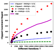
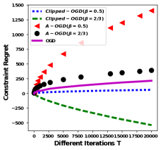
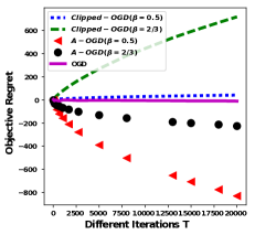
Figure 4: Toy Example Results: Fig.4: Clipped Long-term Constraint Violation. Fig.4: Long-term Constraint Violation. Fig.4: Cumulative Regret of the Loss function

Appendix B Proof of Theorem 1

Before proving Theorem 1, we need the following preliminary result.

Lemma 2.

For the sequence of $x_{t}$, $\lambda_{t}$ obtained from Algorithm 1 and $\forall x\in\mathcal{B}$, we can prove the following inequality:

$$\begin{array}[]{rl}\sum\limits_{t=1}^{T}[\mathcal{L}_{t}(x_{t},\lambda_{t})-\mathcal{L}_{t}(x,\lambda_{t})]&\leq\frac{R^{2}}{2\eta}+\frac{\eta T}{2}(m+1)G^{2}\\ &+\frac{\eta}{2}(m+1)G^{2}\sum\limits_{t=1}^{T}\left\|\lambda_{t}\right\|^{2}\end{array}$$ (13)

Proof.

First, $\mathcal{L}_{t}(x,\lambda)$ is convex in $x$. Then for any $x\in\mathcal{B}$, we have the following inequality:

$$\mathcal{L}_{t}(x_{t},\lambda_{t})-\mathcal{L}_{t}(x,\lambda_{t})\leq(x_{t}-x)^{T}\partial_{x}\mathcal{L}_{t}(x_{t},\lambda_{t})$$ (14)

Using the non-expansive property of the projection operator and the update rule for $x_{t+1}$ in Algorithm 1, we have

$$\begin{array}[]{ll}\left\|x-x_{t+1}\right\|^{2}&\leq\left\|x-(x_{t}-\eta\partial_{x}\mathcal{L}_{t}(x_{t},\lambda_{t}))\right\|^{2}\\ &=\left\|x-x_{t}\right\|^{2}-2\eta(x_{t}-x)^{T}\partial_{x}\mathcal{L}_{t}(x_{t},\lambda_{t})\\ &\quad+\eta^{2}\left\|\partial_{x}\mathcal{L}_{t}(x_{t},\lambda_{t})\right\|^{2}\end{array}$$ (15)

Then we have

$$\small\begin{array}[]{rl}\mathcal{L}_{t}(x_{t},\lambda_{t})-\mathcal{L}_{t}(x,\lambda_{t})&\leq\frac{1}{2\eta}\Big{(}\left\|x-x_{t}\right\|^{2}-\left\|x-x_{t+1}\right\|^{2}\Big{)}\\ &\quad+\frac{\eta}{2}\left\|\partial_{x}\mathcal{L}_{t}(x_{t},\lambda_{t})\right\|^{2}\end{array}$$ (16)

Furthermore, for $\left\|\partial_{x}\mathcal{L}_{t}(x_{t},\lambda_{t})\right\|^{2}$, we have

$$\begin{array}[]{rl}\left\|\partial_{x}\mathcal{L}_{t}(x_{t},\lambda_{t})\right\|^{2}&=\left\|\partial_{x}f_{t}(x_{t})+\sum\limits_{i=1}^{m}\lambda_{t}^{i}\partial_{x}([g_{i}(x_{t})]_{+})\right\|^{2}\\ &\leq(m+1)G^{2}(1+\left\|\lambda_{t}\right\|^{2})\par\end{array}$$ (17)

where the last inequality is from the inequality that $(y_{1}+y_{2}+...+y_{n})^{2}\leq n(y_{1}^{2}+y_{2}^{2}+...+y_{n}^{2})$, and both $\left\|\partial_{x}f_{t}(x_{t})\right|$ and $\left\|\partial_{x}([g_{i}(x_{t})]_{+})\right\|$ are less than or equal to $G$ by the definition.

Then we have

$$\small\begin{array}[]{rl}\mathcal{L}_{t}(x_{t},\lambda_{t})-\mathcal{L}_{t}(x,\lambda_{t})&\leq\frac{1}{2\eta}\Big{(}\left\|x-x_{t}\right\|^{2}-\left\|x-x_{t+1}\right\|^{2}\Big{)}\\ &\quad+\frac{\eta}{2}(m+1)G^{2}(1+\left\|\lambda_{t}\right\|^{2})\par\end{array}$$ (18)

Since $x_{1}$ is in the center of $\mathcal{B}$, we can assume $x_{1}=0$ without loss of generality. If we sum the $\mathcal{L}_{t}(x_{t},\lambda_{t})-\mathcal{L}_{t}(x,\lambda_{t})$ from 1 to $T$, we have

$$\scriptsize\begin{array}[]{ll}\sum\limits_{t=1}^{T}[\mathcal{L}_{t}(x_{t},\lambda_{t})-\mathcal{L}_{t}(x,\lambda_{t})]&\leq\frac{1}{2\eta}\Big{(}\left\|x-x_{1}\right\|^{2}-\left\|x-x_{T+1}\right\|^{2}\Big{)}\\ &\quad+\frac{\eta T}{2}(m+1)G^{2}\\ &\quad+\frac{\eta}{2}(m+1)G^{2}\sum\limits_{t=1}^{T}\left\|\lambda_{t}\right\|^{2}\\ &\leq\frac{R^{2}}{2\eta}+\frac{\eta T}{2}(m+1)G^{2}\\ &\quad+\frac{\eta}{2}(m+1)G^{2}\sum\limits_{t=1}^{T}\left\|\lambda_{t}\right\|^{2}\par\end{array}$$ (19)

where the last inequality follows from the fact that $x_{1}=0$ and $\left\|x\right\|^{2}\leq R^{2}$. ∎

Now we are ready to prove the main theorem.

Proof of Theorem 1.

From Lemma 2, we have

$$\begin{array}[]{rl}\sum\limits_{t=1}^{T}[\mathcal{L}_{t}(x_{t},\lambda_{t})-\mathcal{L}_{t}(x,\lambda_{t})]&\leq\frac{R^{2}}{2\eta}+\frac{\eta T}{2}(m+1)G^{2}\\ &+\frac{\eta}{2}(m+1)G^{2}\sum\limits_{t=1}^{T}\left\|\lambda_{t}\right\|^{2}\end{array}$$ (20)

If we expand the terms in the left-hand side and move the last term in right-hand side to the left, we have

$$\small\begin{array}[]{l}\sum\limits_{t=1}^{T}\Big{(}f_{t}(x_{t})-f_{t}(x)\Big{)}+\sum\limits_{t=1}^{T}\sum\limits_{i=1}^{m}\Big{(}\lambda_{t}^{i}[g_{i}(x_{t})]_{+}-\lambda_{t}^{i}[g_{i}(x)]_{+}\Big{)}\\ -\frac{\eta}{2}(m+1)G^{2}\sum\limits_{t=1}^{T}\left\|\lambda_{t}\right\|^{2}\leq\frac{R^{2}}{2\eta}+\frac{\eta T}{2}(m+1)G^{2}\end{array}$$ (21)

If we set $x=x^{*}$ to have $[g_{i}(x^{*})]_{+}=0$ and plug in the expression $\lambda_{t}=\frac{[g(x_{t})]_{+}}{\sigma\eta}$, we have

$$\small\begin{array}[]{rl}\sum\limits_{t=1}^{T}\Big{(}f_{t}(x_{t})-f_{t}(x^{*})\Big{)}&+\sum\limits_{i=1}^{m}\sum\limits_{t=1}^{T}\frac{([g_{i}(x_{t})]_{+})^{2}}{\sigma\eta}\Big{(}1-\frac{(m+1)G^{2}}{2\sigma}\Big{)}\\ &\leq\frac{R^{2}}{2\eta}+\frac{\eta T}{2}(m+1)G^{2}\par\end{array}$$ (22)

If we plug in the expression for $\sigma$ and $\eta$, we have

$$\small\begin{array}[]{rl}\sum\limits_{t=1}^{T}\Big{(}f_{t}(x_{t})-f_{t}(x^{*})\Big{)}&+\sum\limits_{i=1}^{m}\sum\limits_{t=1}^{T}\frac{([g_{i}(x_{t})]_{+})^{2}}{\sigma\eta}\alpha\\ &\leq O(\sqrt{T})\par\end{array}$$ (23)

Because $\frac{([g_{i}(x_{t})]_{+})^{2}}{\sigma\eta}\alpha\geq 0$, we have

$$\sum\limits_{t=1}^{T}\Big{(}f_{t}(x_{t})-f_{t}(x^{*})\Big{)}\leq O(\sqrt{T})$$ (24)

Furthermore, we have $\sum\limits_{t=1}^{T}\Big{(}f_{t}(x_{t})-f_{t}(x^{*})\Big{)}\geq-FT$ according to the assumption. Then we have

$$\begin{array}[]{l}\sum\limits_{i=1}^{m}\sum\limits_{t=1}^{T}\Big{(}[g_{i}(x_{t})]_{+}\Big{)}^{2}\leq\frac{\sigma\eta}{\alpha}(O(\sqrt{T})+FT)\\ =\frac{\sigma}{\alpha}(O(\sqrt{T})+FT)O(\frac{1}{\sqrt{T}})=O(\sqrt{T})\end{array}$$ (25)

Because $\Big{(}[g_{i}(x_{t})]_{+}\Big{)}^{2}\geq 0$, we have

$$\sum\limits_{t=1}^{T}\Big{(}[g_{i}(x_{t})]_{+}\Big{)}^{2}\leq O(\sqrt{T}),\forall i\in\{1,2,...,m\}$$ (26)

∎

Appendix C Proof of Lemma 1

Proof.

Recall that the update for $x_{t+1}$ is

$$x_{t+1}=\Pi_{\mathcal{B}}\Big{(}x_{t}-\eta\partial_{x}f_{t}(x_{t})-\frac{[g(x_{t})]_{+}}{\sigma}\partial_{x}([g(x_{t})]_{+})\Big{)}$$ (27)

Let $y_{t}=x_{t}-\eta\partial_{x}f_{t}(x_{t})-\frac{[g(x_{t})]_{+}}{\sigma}\partial_{x}([g(x_{t})]_{+})$.

We first need to show that $g(x_{t+1})\leq g(y_{t})$. Without loss of generality, let us assume that $y_{t}$ is not in the set $\mathcal{B}$. From convexity we have $g(y_{t})\geq g(x_{t+1})+\nabla_{x}g(x_{t+1})^{T}(y_{t}-x_{t+1})$. From non-expansiveness of the projection operator, we have that $(y_{t}-x_{t+1})^{T}(x-x_{t+1})\leq 0$ for $x\in\mathcal{B}$. Let $x=x_{t+1}-\epsilon_{0}\nabla_{x}g(x_{t+1})$ with $\epsilon_{0}$ small enough to make $x\in\mathcal{B}$. We have $-\epsilon_{0}(y_{t}-x_{t+1})^{T}\nabla_{x}g(x_{t+1})\leq 0$. Then we have $g(x_{t+1})\leq g(y_{t})$.

As a result, if $g(y_{t})$ is upper bounded, then so is $g(x_{t+1})$, where $x_{t+1}=\Pi_{\mathcal{B}}(y_{t})$. If $T$ is large enough, $\eta\left\|\partial_{x}f_{t}(x_{t})\right\|$ would be very small. Thus, we can use $0$-order Taylor expansion for differentiable $g(x)$ as below:

$$\begin{array}[]{ll}g(y_{t})=&g\Big{(}x_{t}-\eta\partial_{x}f_{t}(x_{t})-\frac{[g(x_{t})]_{+}}{\sigma}\partial_{x}([g(x_{t})]_{+})\Big{)}\\ &\leq g\Big{(}x_{t}-\frac{[g(x_{t})]_{+}}{\sigma}\partial_{x}([g(x_{t})]_{+})\Big{)}+C\eta\end{array}$$ (28)

where $C$ is a constant determined by the Taylor expansion remainder, as well as the bound $\|\partial_{x}[g(x_{t})]_{+}\|\|\partial_{X}f(x_{t})\|\leq G^{2}$.

Set $\epsilon=(2C\sigma R^{2}\eta)^{1/3}=O(\frac{1}{T^{1/6}})$. We will show that if $g(x_{t})<\epsilon$, then $g(x_{t+1})\leq\epsilon+O(1/\sqrt{T})=O(\frac{1}{T^{1/6}})$. We will also show that if $g(x_{t})\geq\epsilon$, then $g(x_{t+1})\leq g(x_{t})$. It follows then by induction that if $g(x_{1})<\epsilon$, then $g(x_{t})=O(\frac{1}{T^{1/6}})$ for all $t$. We prove these inequalities in three cases. Since $g(x_{t+1})\leq g(y_{t})$, it suffices to bound $g(y_{t})$.

Case 1: $g(x_{t})\leq 0$. In this case, the inequality for $g(y_{t})$, (28), becomes

$$g(y_{t})\leq g(x_{t})+C\eta\leq C\eta=O(\frac{1}{\sqrt{T}})$$ (29)

Case 2: $0<g(x_{t})<\epsilon$. Since $[g(x_{t})]_{+}=g(x_{t})$, the bound on $g(y_{t})$ becomes

$$g(y_{t})\leq g\Big{(}x_{t}-\frac{g(x_{t})}{\sigma}\nabla_{x}g(x_{t})\Big{)}+C\eta$$ (30)

We will bound the right using standard methods from gradient descent proofs. Since $g$ is convex and $\nabla_{x}g(x)$ has Lipschitz constant, $L$, we have the inequality:

$$g(y)\leq g(x)+\nabla_{x}g(x)^{T}(y-x)+\frac{L}{2}\|y-x\|^{2}$$ (31)

for all $x$ and $y$ Nesterov [2013].

Recall that $\epsilon=O(\frac{1}{T^{1/6}})$. Assume that $T$ is sufficiently large so that $\frac{Lg(x_{t})}{2\sigma}<\frac{L\epsilon}{2\sigma}<1$. Applying (31) with $x=x_{t}$ and $y=x_{t}-\frac{g(x_{t})}{\sigma}\nabla_{x}g(x_{t})$ gives

$$g(y_{t}) \leq g\Big{(}x_{t}-\frac{[g(x_{t})]_{+}}{\sigma}\partial_{x}(g(x_{t}))\Big{)}+C\eta$$ (32)

$$\leq g(x_{t})-\frac{g(x_{t})}{\sigma}(1-\frac{Lg(x_{t})}{2\sigma})\left\|\nabla_{x}g(x_{t})\right\|^{2}+C\eta$$ (33)

$$\leq g(x_{t})+C\eta=O(\frac{1}{T^{1/6}}).$$ (34)

where the third bound follows since $1-\frac{Lg(x_{t})}{2\sigma}>0$.

Case 3: $g(x_{t})\geq\epsilon$. A case can arise such that $g(x_{t-1})<\epsilon$ but an additive term of order $O(\frac{1}{T^{1/2}})$ leads to $\epsilon\leq g(x_{t})\leq\epsilon+C\eta=O(\frac{1}{T^{1/6}})$. We will now show that no further increases are possible by bounding the final two terms of (33) as

$$-\frac{g(x_{t})}{\sigma}(1-\frac{Lg(x_{t})}{2\sigma})\left\|\nabla_{x}g(x_{t})\right\|^{2}+C\eta\leq 0\iff C\eta\leq\frac{g(x_{t})}{\sigma}(1-\frac{Lg(x_{t})}{2\sigma})\left\|\nabla_{x}g(x_{t})\right\|^{2}.$$ (35)

Now, we lower-bound the terms on the right of (35). Since $\epsilon+C\eta=O(\frac{1}{T^{1/6}})$, we have that for sufficiently large $T$, $1-\frac{Lg(x_{t})}{2\sigma}\geq 1-\frac{L(\epsilon+C\eta)}{2\sigma}\geq\frac{1}{2}$. Further note that by convexity, $g(0)\geq g(x_{t})-\nabla_{x}g(x_{t})^{T}x_{t}$. Since we assume that $0$ is feasible, we have that

$$\epsilon\leq g(x_{t})\leq\nabla_{x}g(x_{t})^{T}x_{t}\leq\|\nabla_{x}g(x_{t})\|\|x_{t}\|\leq\|\nabla_{x}g(x_{t})\|R.$$

The final inequality follows since $x_{t}\in\mathcal{B}$. Thus, we have the following bound for the right of (35):

$$\frac{g(x_{t})}{\sigma}(1-\frac{Lg(x_{t})}{2\sigma})\left\|\nabla_{x}g(x_{t})\right\|^{2}\geq\frac{\epsilon^{3}}{2\sigma R^{2}}=C\eta.$$

The final equality follows by the definition of $\epsilon$. ∎

Appendix D Proof of Theorem 2

Proof.

For the strongly convex case of $f_{t}(x)$ with strong convexity parameter equal to $H_{1}$, we can also conclude that the modified augmented Lagrangian function in Eq.(8) is also strongly convex w.r.t. $x$ with the strong convexity parameter $H\geq H_{1}$. Then we have

$$\begin{array}[]{rl}\mathcal{L}_{t}(x^{*},\lambda_{t})-\mathcal{L}_{t}(x_{t},\lambda_{t})&\geq\partial_{x}\mathcal{L}_{t}(x_{t})^{T}(x^{*}-x_{t})\\ &+\frac{H_{1}}{2}\left\|x^{*}-x_{t}\right\|^{2}\end{array}$$ (36)

From concavity of $\mathcal{L}$ in terms of $\lambda$, we can have

$$\mathcal{L}_{t}(x_{t},\lambda)-\mathcal{L}_{t}(x_{t},\lambda_{t})\leq(\lambda-\lambda_{t})^{T}\nabla_{\lambda}\mathcal{L}_{t}(x_{t},\lambda_{t})$$ (37)

Since $\lambda_{t}$ maximizes the augmented Lagrangian, we can see that the right hand side is $0$.

From Eq.(15), we have

$$\begin{array}[]{rl}\partial_{x}\mathcal{L}_{t}(x_{t})^{T}(x_{t}-x^{*})\leq&\frac{1}{2\eta_{t}}\Big{(}\left\|x^{*}-x_{t}\right\|^{2}-\left\|x^{*}-x_{t+1}\right\|^{2}\Big{)}\\ &+\frac{\eta_{t}}{2}(m+1)G^{2}(1+\left\|\lambda_{t}\right\|^{2})\par\end{array}$$ (38)

Multiply Eq.(36) by $-1$ and add Eq.(37) together with Eq.(38) plugging in:

$$\begin{array}[]{l}\mathcal{L}_{t}(x_{t},\lambda)-\mathcal{L}_{t}(x^{*},\lambda_{t})\leq\frac{1}{2\eta_{t}}\Big{(}\left\|x^{*}-x_{t}\right\|^{2}-\left\|x^{*}-x_{t+1}\right\|^{2}\Big{)}\\ \quad+\frac{\eta_{t}}{2}(m+1)G^{2}(1+\left\|\lambda_{t}\right\|^{2})-\frac{H_{1}}{2}\left\|x^{*}-x_{t}\right\|^{2}\end{array}$$ (39)

Let $b_{t}=\left\|x^{*}-x_{t}\right\|^{2}$, and plug in the expression for $\mathcal{L}_{t}$, we can get:

$$\begin{array}[]{l}f_{t}(x_{t})-f_{t}(x^{*})+\lambda^{T}[g(x_{t})]_{+}-\frac{\theta_{t}}{2}\left\|\lambda\right\|^{2}\leq\frac{1}{2\eta_{t}}(b_{t}-b_{t+1})\\ \quad-\frac{H_{1}}{2}b_{t}+\frac{(m+1)G^{2}}{2}\eta_{t}+\frac{(m+1)G^{2}}{2}\left\|\lambda_{t}\right\|^{2}(\eta_{t}-\frac{\theta_{t}}{(m+1)G^{2}})\end{array}$$ (40)

Plug in the expressions $\eta_{t}=\frac{1}{H_{1}(t+1)}$, $\theta_{t}=(m+1)G^{2}\eta_{t}$, and sum over $t=1$ to $T$:

$$\begin{array}[]{l}\sum\limits_{t=1}^{T}\Big{(}f_{t}(x_{t})-f_{t}(x^{*})\Big{)}+\lambda^{T}\Big{(}\sum\limits_{t=1}^{T}[g(x_{t})]_{+}\Big{)}-\frac{\left\|\lambda\right\|^{2}}{2}\sum\limits_{t=1}^{T}\theta_{t}\\ \leq\underbrace{\frac{1}{2}\sum\limits_{t=1}^{T}\Big{(}\frac{b_{t}-b_{t+1}}{\eta_{t}}-\frac{H_{1}}{2}b_{t}\Big{)}}_{A}+\underbrace{\frac{(m+1)G^{2}}{2}\sum\limits_{t=1}^{T}\eta_{t}}_{B}\end{array}$$ (41)

For the expression of $A$, we have:

$$\begin{array}[]{l}A=\frac{1}{2}\Big{[}\frac{b_{1}}{\eta_{1}}+\sum\limits_{t=2}^{T}b_{t}(\frac{1}{\eta_{t}}-\frac{1}{\eta_{t-1}}-H_{1})-\frac{b_{T+1}}{\eta_{T}}-H_{1}b_{1}\Big{]}\\ \quad\leq b_{1}H_{1}\end{array}$$ (42)

For the expression of $B$, with the expression of $\eta_{t}$ and the inequality relation between sum and integral, we have:

$$B\leq\frac{(m+1)G^{2}}{2H_{1}}\log(T)$$ (43)

Thus, we have:

$$\begin{array}[]{l}\sum\limits_{t=1}^{T}\Big{(}f_{t}(x_{t})-f_{t}(x^{*})\Big{)}+\lambda^{T}\Big{(}\sum\limits_{t=1}^{T}[g(x_{t})]_{+}\Big{)}-\frac{\left\|\lambda\right\|^{2}}{2}\sum\limits_{t=1}^{T}\theta_{t}\\ \leq O(\log(T))\end{array}$$ (44)

If we set $\lambda=\frac{\sum\limits_{t=1}^{T}[g(x_{t})]_{+}}{\sum\limits_{t=1}^{T}\theta_{t}}$, and due to non-negativity of $\frac{\Big{\|}\sum\limits_{t=1}^{T}[g(x_{t})]_{+}\Big{\|}^{2}}{2\sum\limits_{t=1}^{T}\theta_{t}}$, we can have

$$\sum\limits_{t=1}^{T}\Big{(}f_{t}(x_{t})-f_{t}(x^{*})\Big{)}\leq O(\log(T))$$ (45)

Furthermore, we have $\sum\limits_{t=1}^{T}\Big{(}f_{t}(x_{t})-f_{t}(x^{*})\Big{)}\geq-FT$ according to the assumption. Then we have

$$\frac{\Big{\|}\sum\limits_{t=1}^{T}[g(x_{t})]_{+}\Big{\|}^{2}}{2\sum\limits_{t=1}^{T}\theta_{t}}\leq O(\log(T))+FT$$ (46)

Because $\sum\limits_{t=1}^{T}\theta_{t}\leq(m+1)G^{2}\log(T)/H_{1}$, we have:

$$\big{\|}\sum\limits_{t=1}^{T}[g(x_{t})]_{+}\big{\|}\leq O(\sqrt{\log(T)T})$$ (47)

∎

Appendix E Proof of the Propositions

Now we give the proofs for all the remaining Propositions.

Proof of the Proposition 1.

From the construction of $\bar{g}(x)$, we have the $\bar{g}(x)\geq\max\limits_{i}g_{i}(x)$. Thus, if we can upper bound the $\bar{g}(x)$, $g_{i}(x)$ will automatically be upper bounded. In order to use Lemma 1, we need to make sure the following conditions are satisfied:

• $\bar{g}(x)$ is convex and differentiable.

• $\left\|\nabla_{x}\bar{g}(x)\right\|$ is upper bounded.

• $\left\|\nabla_{x}^{\prime\prime}\bar{g}(x)\right\|_{2}$ is upper bounded.

The first condition is satisfied due to the formula of $\bar{g}(x)$. To examine the second one, we have

$$\nabla_{x}\bar{g}(x)=\frac{1}{\sum\limits_{i=1}^{m}\exp g_{i}(x)}\Bigg{[}\sum\limits_{i=1}^{m}\exp g_{i}(x)\nabla_{x}g_{i}(x)\Bigg{]}$$ (48)

$$\begin{array}[]{rl}\left\|\nabla_{x}\bar{g}(x)\right\|^{2}&=\frac{1}{\big{(}\sum\limits_{i=1}^{m}\exp g_{i}(x)\big{)}^{2}}\left\|\sum\limits_{i=1}^{m}\exp g_{i}(x)\nabla_{x}g_{i}(x)\right\|^{2}\\ &\leq\frac{m\sum\limits_{i=1}^{m}(\exp g_{i}(x))^{2}\left\|\nabla_{x}g_{i}(x)\right\|^{2}}{\big{(}\sum\limits_{i=1}^{m}\exp g_{i}(x)\big{)}^{2}}\\ &\leq mG^{2}\end{array}$$ (49)

Thus, $\left\|\nabla_{x}\bar{g}(x)\right\|\leq\sqrt{m}G$ and the second condition is satisfied.

For $\left\|\nabla_{x}^{\prime\prime}\bar{g}(x)\right\|_{2}$, we have

$$\begin{array}[]{ll}\nabla_{x}^{\prime\prime}\bar{g}(x)=&\underbrace{\frac{1}{\sum\limits_{i=1}^{m}\exp g_{i}(x)}\Bigg{[}\sum\limits_{i=1}^{m}\exp g_{i}(x)\nabla_{x}^{\prime\prime}g_{i}(x)+\exp g_{i}(x)\nabla_{x}g_{i}(x)\nabla_{x}g_{i}(x)^{T}\Bigg{]}}_{A}\\ &-\underbrace{\frac{1}{\sum\limits_{i=1}^{m}\exp g_{i}(x)}\Big{(}\sum\limits_{i=1}^{m}\exp g_{i}(x)\nabla_{x}g_{i}(x)\Big{)}\Big{(}\sum\limits_{i=1}^{m}\exp g_{i}(x)\nabla_{x}g_{i}(x)^{T}\Big{)}}_{B}\end{array}$$ (50)

To upper bound $\left\|\nabla_{x}^{\prime\prime}\bar{g}(x)\right\|_{2}$, which is

$$\max\limits_{u^{T}u=1}u^{T}\nabla_{x}^{\prime\prime}\bar{g}(x)u=\max\limits_{u^{T}u=1}u^{T}Au-u^{T}Bu\leq\max\limits_{u^{T}u=1}u^{T}Au$$ (51)

where the inequality is due to the fact that $B\succeq 0$.

Thus, we have $\left\|\nabla_{x}^{\prime\prime}\bar{g}(x)\right\|_{2}\leq\left\|A\right\|_{2}$. For the $\left\|A\right\|_{2}$, we have

$$\begin{array}[]{ll}\left\|A\right\|_{2}=&\max\limits_{u^{T}u=1}u^{T}Au\leq\frac{1}{\sum\limits_{i=1}^{m}\exp g_{i}(x)}\Big{(}\sum\limits_{i=1}^{m}\max\limits_{u^{T}u=1}\exp g_{i}(x)u^{T}\nabla_{x}^{\prime\prime}g_{i}(x)u\Big{)}\\ &+\frac{1}{\sum\limits_{i=1}^{m}\exp g_{i}(x)}\Big{(}\sum\limits_{i=1}^{m}\max\limits_{u^{T}u=1}\exp g_{i}(x)\left\|\nabla_{x}g_{i}(x)^{T}u\right\|^{2}\Big{)}\\ &\leq\frac{1}{\sum\limits_{i=1}^{m}\exp g_{i}(x)}\Big{(}\sum\limits_{i=1}^{m}\exp g_{i}(x)(L_{i}+\left\|\nabla_{x}g_{i}(x)\right\|^{2})\Big{)}\\ &\leq\frac{1}{\sum\limits_{i=1}^{m}\exp g_{i}(x)}\Big{(}\sum\limits_{i=1}^{m}\exp g_{i}(x)\Big{)}(\bar{L}+G^{2})=\bar{L}+G^{2}\end{array}$$ (52)

where the first inequality comes from the optimality definition, the second inequality comes from the upper bound for each $\left\|\nabla_{x}^{\prime\prime}g_{i}(x)\right\|_{2}$ and the Cauchy - Schwartz inequality, and the last inequality comes from the fact that $\bar{L}=\max L_{i}$ and $\left\|\nabla_{x}g_{i}(x)\right\|$ is upper bounded by $G$. Thus, the last condition is also satisfied. ∎

Proof of the Proposition 2.

From Theorem 1, we know that $\sum\limits_{t=1}^{T}\Big{(}[g_{i}(x_{t})]_{+}\Big{)}^{2}\leq O(\sqrt{T})$. By using the inequality $(y_{1}+y_{2}+...+y_{n})^{2}\leq n(y_{1}^{2}+y_{2}^{2}+...+y_{n}^{2})$, setting $y_{i}$ being equal to $[g_{i}(x_{t})]_{+}$, and $n=T$, we have $\Big{(}\sum\limits_{t=1}^{T}[g_{i}(x_{t})]_{+}\Big{)}^{2}\leq T\sum\limits_{t=1}^{T}\Big{(}[g_{i}(x_{t})]_{+}\Big{)}^{2}\leq O(T^{3/2})$. Then we obtain that $\sum\limits_{t=1}^{T}[g_{i}(x_{t})]_{+}\leq O(T^{3/4})$. Because $g_{i}(x_{t})\leq[g_{i}(x_{t})]_{+}$, we also have $g_{i}(x_{t})\leq O(T^{3/4})$. ∎

Proof of the Proposition 3.

Since we only change the stepsize for Algorithm 1, the previous result in Lemma 2 and part of the proof up to Eq.(22) in Theorem 1 can be used without any changes.

First, let us rewrite the Eq.(22):

$$\small\begin{array}[]{rl}\sum\limits_{t=1}^{T}\Big{(}f_{t}(x_{t})-f_{t}(x^{*})\Big{)}&+\sum\limits_{i=1}^{m}\sum\limits_{t=1}^{T}\frac{([g_{i}(x_{t})]_{+})^{2}}{\sigma\eta}\Big{(}1-\frac{(m+1)G^{2}}{2\sigma}\Big{)}\\ &\leq\frac{R^{2}}{2\eta}+\frac{\eta T}{2}(m+1)G^{2}\par\end{array}$$ (53)

By plugging in the definition of $\alpha$, $\eta$, and that $\frac{([g_{i}(x_{t})]_{+})^{2}}{\sigma\eta}\alpha\geq 0$, we have

$$\begin{array}[]{ll}\sum\limits_{t=1}^{T}\Big{(}f_{t}(x_{t})-f_{t}(x^{*})\Big{)}&\leq\frac{R^{2}}{2}T^{\beta}+\frac{(m+1)G^{2}}{2}T^{1-\beta}\\ &=O(T^{max\{\beta,1-\beta\}})\end{array}$$ (54)

As argued in the proof of Theorem 1, we have the following inequality with the help of $\sum\limits_{t=1}^{T}\Big{(}f_{t}(x_{t})-f_{t}(x^{*})\Big{)}\geq-FT$:

$$\begin{array}[]{l}\sum\limits_{i=1}^{m}\sum\limits_{t=1}^{T}\frac{([g_{i}(x_{t})]_{+})^{2}}{\sigma\eta}\alpha\leq\frac{R^{2}}{2}T^{\beta}+\frac{(m+1)G^{2}}{2}T^{1-\beta}+FT\\ \sum\limits_{t=1}^{T}([g_{i}(x_{t})]_{+})^{2}\leq\frac{\sigma}{\alpha}(\frac{R^{2}}{2}+\frac{(m+1)G^{2}}{2}T^{1-2\beta}+FT^{1-\beta})\par\end{array}$$ (55)

Then we have

$$\begin{array}[]{l}\sum\limits_{t=1}^{T}[g_{i}(x_{t})]_{+}\leq\sqrt{T\sum\limits_{t=1}^{T}\Big{(}[g_{i}(x_{t})]_{+}\Big{)}^{2}}\\ \leq\sqrt{\frac{T\sigma}{\alpha}\Big{(}\frac{R^{2}}{2}+\frac{(m+1)G^{2}}{2}T^{1-2\beta}+FT^{1-\beta}\Big{)}}\\ =O(T^{1-\beta/2})\end{array}$$ (56)

∎

It is also interesting to figure out why Mahdavi et al. [2012] cannot have this user-defined trade-off benefit. From Mahdavi et al. [2012], the key inequality in obtaining their conclusions is:

$$\begin{array}[]{l}\sum\limits_{t=1}^{T}\Big{(}f_{t}(x_{t})-f_{t}(x^{*})\Big{)}+\sum\limits_{i=1}^{m}\frac{\Big{[}\sum\limits_{t=1}^{T}g_{i}(x_{t})\Big{]}_{+}^{2}}{2(\sigma\eta T+m/\eta)}\\ \leq\frac{R^{2}}{2\eta}+\frac{\eta T}{2}\Big{(}(m+1)G^{2}+2mD^{2}\Big{)}\end{array}$$ (57)

The main difference between Eq.(57) and Eq.(53) is in the denominator of $\frac{\Big{[}\sum\limits_{t=1}^{T}g_{i}(x_{t})\Big{]}_{+}^{2}}{2(\sigma\eta T+m/\eta)}$. Eq.(57) has the form $(\sigma\eta T+m/\eta)$, while Eq.(53) has the form $(\sigma\eta)$. The coupled $\eta$ and $1/\eta$ prevents Eq.(57) from arriving this user-defined trade-off.

The next proofs of the Proposition 4 and 5 show how we can use our proposed Lagrangian function in Eq.(7) to make the algorithms in Mahdavi et al. [2012] and Jenatton et al. [2016] to have the clipped long-term constraint violation bounds.

Proof of the Proposition 4.

If we look into the proof of Lemma 2 and Proposition 3 in Mahdavi et al. [2012], the new Lagrangian formula does not lead to any difference, which means that the $\mathcal{L}_{t}(x,\lambda)$ defined in Eq.(7) is also valid for the drawn conclusions. Then in the proof of Theorem 4 in Mahdavi et al. [2012], we can change $g_{i}(x_{t})$ to $[g_{i}(x_{t})]_{+}$. The maximization for $\lambda$ over the range $[0,+\infty)$ is also valid, since $[g_{i}(x_{t})]_{+}$ automatically satisfies this requirement. Thus, the claimed bounds hold. ∎

Proof of the Proposition 5.

The previous augmented Lagrangian formula $\mathcal{L}_{t}(x,\lambda)$ used in Jenatton et al. [2016] is:

$$\mathcal{L}_{t}(x,\lambda)=f_{t}(x)+\lambda g(x)-\frac{\theta_{t}}{2}\lambda^{2}$$ (58)

The Lemma 1 in Jenatton et al. [2016] is the upper bound of $\mathcal{L}_{t}(x_{t},\lambda)-\mathcal{L}_{t}(x_{t},\lambda_{t})$. The proof does not make any difference between formula (58) and (9). So we can still have the same conclusion of Lemma 1. The Lemma 2 in Jenatton et al. [2016] is the lower bound of $\mathcal{L}_{t}(x_{t},\lambda)-\mathcal{L}_{t}(x^{*},\lambda_{t})$. Since it only uses the fact that $g(x^{*})\leq 0$, which is also true for $[g(x^{*})]_{+}$, we can have the same result with $g(x_{t})$ being replaced with $[g(x_{t})]_{+}$. The Lemma 3 in Jenatton et al. [2016] is free of $\mathcal{L}_{t}(x,\lambda)$ formula, so it is also true for the new formula. The Lemma 4 in Jenatton et al. [2016] is the result of Lemma 1-3, so it is also valid if we change $g(x_{t})$ to $[g(x_{t})]_{+}$. Then the conclusion of Theorem 1 in Jenatton et al. [2016] is valid for $[g(x_{t})]_{+}$ as well. ∎

References

- Blum et al. (2004) Avrim Blum, Vijay Kumar, Atri Rudra, and Felix Wu. Online learning in online auctions. Theoretical Computer Science, 324(2-3):137–146, 2004.
- Cesa-Bianchi and Lugosi (2006) Nicolo Cesa-Bianchi and Gábor Lugosi. Prediction, learning, and games. Cambridge university press, 2006.
- Crammer et al. (2006) Koby Crammer, Ofer Dekel, Joseph Keshet, Shai Shalev-Shwartz, and Yoram Singer. Online passive-aggressive algorithms. Journal of Machine Learning Research, 7(Mar):551–585, 2006.
- Defazio et al. (2014) Aaron Defazio, Francis Bach, and Simon Lacoste-Julien. Saga: A fast incremental gradient method with support for non-strongly convex composite objectives. In Advances in Neural Information Processing Systems, pages 1646–1654, 2014.
- Diamond and Boyd (2016) Steven Diamond and Stephen Boyd. CVXPY: A Python-embedded modeling language for convex optimization. Journal of Machine Learning Research, 17(83):1–5, 2016.
- Duchi et al. (2008) John Duchi, Shai Shalev-Shwartz, Yoram Singer, and Tushar Chandra. Efficient projections onto the l 1-ball for learning in high dimensions. In Proceedings of the 25th international conference on Machine learning, pages 272–279. ACM, 2008.
- Duchi et al. (2010) John C Duchi, Shai Shalev-Shwartz, Yoram Singer, and Ambuj Tewari. Composite objective mirror descent. In COLT, pages 14–26, 2010.
- Fazel et al. (2018) Maryam Fazel, Rong Ge, Sham M Kakade, and Mehran Mesbahi. Global convergence of policy gradient methods for linearized control problems. arXiv preprint arXiv:1801.05039, 2018.
- Hazan et al. (2007) Elad Hazan, Amit Agarwal, and Satyen Kale. Logarithmic regret algorithms for online convex optimization. Machine Learning, 69(2):169–192, 2007.
- Jenatton et al. (2016) Rodolphe Jenatton, Jim Huang, and Cédric Archambeau. Adaptive algorithms for online convex optimization with long-term constraints. In International Conference on Machine Learning, pages 402–411, 2016.
- LeCun et al. (1998) Yann LeCun, Léon Bottou, Yoshua Bengio, and Patrick Haffner. Gradient-based learning applied to document recognition. Proceedings of the IEEE, 86(11):2278–2324, 1998.
- Li et al. (2018) Yingying Li, Guannan Qu, and Na Li. Online optimization with predictions and switching costs: Fast algorithms and the fundamental limit. arXiv preprint arXiv:1801.07780, 2018.
- Mahdavi et al. (2012) Mehrdad Mahdavi, Rong Jin, and Tianbao Yang. Trading regret for efficiency: online convex optimization with long term constraints. Journal of Machine Learning Research, 13(Sep):2503–2528, 2012.
- Mairal et al. (2009) Julien Mairal, Francis Bach, Jean Ponce, and Guillermo Sapiro. Online dictionary learning for sparse coding. In Proceedings of the 26th annual international conference on machine learning, pages 689–696. ACM, 2009.
- Mnih et al. (2015) Volodymyr Mnih, Koray Kavukcuoglu, David Silver, Andrei A Rusu, Joel Veness, Marc G Bellemare, Alex Graves, Martin Riedmiller, Andreas K Fidjeland, Georg Ostrovski, et al. Human-level control through deep reinforcement learning. Nature, 518(7540):529–533, 2015.
- Nesterov (2005) Yu Nesterov. Smooth minimization of non-smooth functions. Mathematical programming, 103(1):127–152, 2005.
- Nesterov (2013) Yurii Nesterov. Introductory lectures on convex optimization: A basic course, volume 87. Springer Science & Business Media, 2013.
- Senthil and Manikandan (2010) K Senthil and K Manikandan. Economic thermal power dispatch with emission constraint and valve point effect loading using improved tabu search algorithm. International Journal of Computer Applications, 2010.
- Yu et al. (2017) Hao Yu, Michael Neely, and Xiaohan Wei. Online convex optimization with stochastic constraints. In Advances in Neural Information Processing Systems, pages 1427–1437, 2017.
- Yuan and Lamperski (2017) Jianjun Yuan and Andrew Lamperski. Online control basis selection by a regularized actor critic algorithm. In American Control Conference (ACC), 2017, pages 4448–4453. IEEE, 2017.
- Zinkevich (2003) Martin Zinkevich. Online convex programming and generalized infinitesimal gradient ascent. In Proceedings of the 20th International Conference on Machine Learning (ICML-03), pages 928–936, 2003.
Supplemental Materials