Multicritical edge statistics for the momenta of fermions in non-harmonic traps

Abstract

We compute the joint statistics of the momenta $p_{i}$ of $N$ non-interacting fermions in a trap, near the Fermi edge, with a particular focus on the largest one $p_{\max}$. For a $1d$ harmonic trap, momenta and positions play a symmetric role and hence, the joint statistics of momenta is identical to that of the positions. In particular, $p_{\max}$, as $x_{\max}$, is distributed according to the Tracy-Widom distribution. Here we show that novel “momentum edge statistics” emerge when the curvature of the potential vanishes, i.e. for ”flat traps” near their minimum, with $V(x)\sim x^{2n}$ and $n>1$. These are based on generalisations of the Airy kernel that we obtain explicitly. The fluctuations of $p_{\max}$ are governed by new universal distributions determined from the $n$-th member of the second Painlevé hierarchy of non-linear differential equations, with connections to multicritical random matrix models. Finite temperature extensions and possible experimental signatures in cold atoms are discussed.

Fermi gases in confining traps exhibit an edge in space, where the density vanishes GPS08 ; BDZ08 ; castin . As a result, the quantum and thermal fluctuations are greatly enhanced leading to interesting edge physics. The case of spinless non-interacting fermions is more tractable analytically: recently a number of theoretical predictions, at zero and finite temperature, were obtained Kohn ; Eis2013 ; us_finiteT ; DPMS:2015 ; fermions_review ; Dubail . These are ripe to be tested in cold atom experiments where the non-interacting limit can be reached Chin2010 ; 2DBoxGaz . Two complementary experiments are possible, either the quantum microscopes, which measure jointly the positions $x_{i}$ of the fermions Cheuk:2015 ; Haller:2015 ; Parsons:2015 ; Omran2015 , or the time of flight experiments which measure jointly their momenta $p_{i}$ TOF ; 2DBoxGaz .

Most of the recent predictions concern the positions $x_{i}$ of $N$ noninteracting fermions. At zero temperature, $T=0$, in one dimension, $d=1$, and for a harmonic trap, $V(x)=\frac{1}{2}m\omega^{2}x^{2}$, they are in one-to-one correspondence Eis2013 ; us_finiteT ; marino_prl ; CMV2011 ; CDM14 ; castillo with the eigenvalues of a complex Hermitian matrix with independent Gaussian entries, known as the Gaussian Unitary Ensemble (GUE) of random matrix theory mehta ; forrester . Their joint probability distribution function (PDF) is given by the Wigner-Dyson formula. The fermion density is thus the Wigner semi-circle which vanishes at the edge $x_{e}$ as $\rho(x)\sim|x-x_{e}|^{1/2}$. Consequently, the spatial quantum correlations at the edge of the trap are described by the fluctuations of the few largest eigenvalues of the GUE fermions_review . These form a determinantal point process johansson ; borodin_determinantal ; tracy_widom_determinantal , i.e all correlation functions can be written as determinants with entries called kernel.

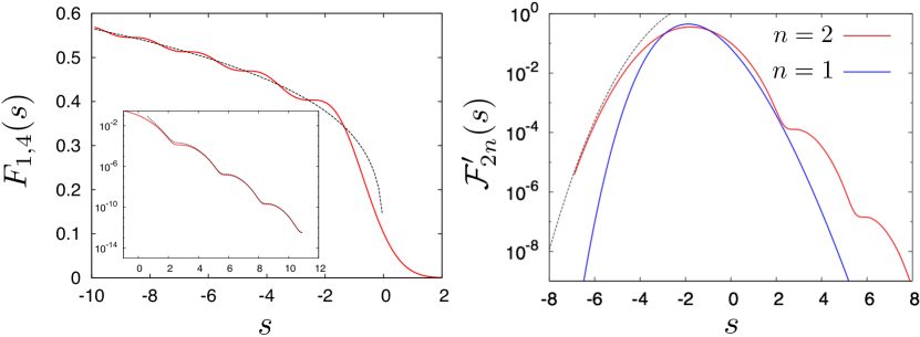
Figure 1: Left: Solid line: scaling function $F_{1,2n=4}(s)$, Eq. (4), of the density at the edge, for $V(x)\sim x^{4}$. Dotted line: $s\to-\infty$ asymptotics $F_{1,4}(s)\simeq\frac{|s|^{1/4}}{\pi}$, matching the bulk density, see above (4). Inset: same in log-linear scale showing the large $s>0$ oscillations. Dotted line: asymptotics in (6). Right: Scaling function ${\cal F}^{\prime}_{2n}(s)$ of the PDF of $p_{\max}$ in (8)-(10). Red: $n=2$. Blue: the TW distribution ($n=1$) for comparison. Dotted line: large $s<0$ behavior, ${\cal F}^{\prime}_{4}(s)\sim\exp(-\frac{\sqrt{8/3}}{15}|s|^{5/2})$.

In the case of GUE, this kernel is called the Airy kernel TracyWidomAiry , as it is related to the Green’s function of a single quantum particle in a linear potential. In particular the PDF of the (properly centered and scaled) position of the rightmost fermions $x_{\max}=\max_{i=1,\ldots,N}x_{i}$ is given us_finiteT by the celebrated GUE Tracy Widom (TW) distribution TracyWidomAiry , which also arises in many problems in mathematics and physics baik ; johann ; growth ; CLR10 ; DOT10 ; ACQ11 ; sequence ; MS_thirdorder and was measured in experiments takeuchi ; davidson ; lemarie in other contexts. These properties were shown to extend to finite temperature, in terms of a one-parameter deformation of the Airy kernel, indexed by the reduced temperature $b=\hbar\omega N^{1/3}/T$ (with a corresponding finite $T$ extension of the TW distribution) us_finiteT ; fermions_review ; LiechtyT . Remarkably, these spatial edge correlations were shown to be universal, independent of the details of the smooth confining potential Eis2013 ; fermions_review , which can be traced to the fact that the density at the edge still vanishes as $|x-x_{e}|^{1/2}$. Extensions to dimensions $d>1$  DPMS:2015 ; farthest_f ; torquato and non-smooth potentials, e. g. hard box FFGW03 ; Cunden1D ; UsHardBox , were also studied.

One can now ask about the statistics of the momenta $p_{i}$ of $N$ non interacting fermions, and their maximum $p_{\max}=\max_{i=1,\ldots,N}p_{i}$, in a (e.g. $1d$) trap described by a single particle Hamiltonian $H=\frac{p^{2}}{2m}+V(x)$. It is an important question to make predictions for time of flight experiments in traps of varying shapes, as can be currently designed BDZ08 ; Zwi2017 ; 2DBoxGaz . If the potential is bounded from below, there exists also an edge in momentum space $p_{e}$, beyond which the momentum density vanishes. Obviously, if the confining potential is harmonic, momenta and positions play a symmetric role and the two (dimensionless) random sets $\{p_{i}/\hbar\alpha\}_{i=1,\ldots,N}$ (momenta) and $\{\alpha x_{i}\}_{i=1,\ldots,N}$ (coordinates) are described by exactly the same joint PDF (here $\alpha=\sqrt{m\omega/\hbar}$ is the harmonic oscillator inverse length scale), at any temperature (and, in fact, in any $d$). The question of what happens for a more general, non harmonic trap, $V(x)\sim x^{2n}$ is however, non-trivial and open. Interestingly, as we find below, the density in momentum space vanishes as

$$\rho(p)\sim(p_{e}-p)^{\frac{1}{2n}}\;,$$ (1)

i.e, distinct from the standard Wigner semi-circle exponent $\frac{1}{2}$ (for $n=1$) which suggests a new universality class. In particular we expect that the fluctuations of $p_{\max}$ are given by a distribution different from the TW.

On the random matrix side, there exist generalizations of the GUE involving matrix potentials such that the density of eigenvalues vanishes at the edge with a rational exponent ${\sf q}/{\sf p}$ ReviewMatrixModels . In the so-called double scaling limit gross1990nonperturbative ; douglas1990strings ; brezin1990exactly ; BowickBrezin , these matrix models exhibit multicritical points indexed by two integers $({\sf p},{\sf q})$ with universal properties BrezinHouches ; KazakovDaul ; Eynard ; BrezinHikamiSource ; janik ; AkemanNew . Such models were introduced in the context of random surfaces and string theory BIPZ ; GrossWitten ; Periwal1 ; Douglas ; Mandal1 ; Mandal2 ; Douglas2 ; Klebanov ; marino . A special class of these models were recently studied in Claes1 ; Gernot_TW , leading to generalizations of the TW distribution. A natural question is whether there are experimentally relevant settings where the universal physics near these multicritical points can be accessed. Given the behavior of the density (1), the momentum statistics of fermions near the edge may be a natural candidate.

Indeed, in this paper we demonstrate that the momentum statistics at the edge of noninteracting fermions in some non-harmonic potentials (i) leads to universality classes different from the GUE-TW class (ii) appears to be in correspondence with a class of multicritical matrix models. We focus on $d=1$ and consider potentials which (with no loss of generality) attain their minimum at $x=0$, i.e. $V(0)=V_{\min}=\min_{x}V(x)=0$. Two edges in momentum space then exist at $\pm p_{e}$ with $p_{e}=\sqrt{2m\mu}$, $\mu$ being the Fermi energy. We show that the set of momenta $\{p_{i}\}_{i=1,\ldots,N}$ forms a determinantal point process, which, near the edges, is characterized by universal kernels. The universality classes however depend on the behavior of the potential near its minimum. If the curvature there is non-zero, the universality class is the one of the Airy kernel (e.g. leading to the TW distribution for properly centered and scaled $p_{\max}$). If the curvature vanishes, e.g. if $V(x)\sim x^{2n}$ with $n>1$, which is the case e.g. for the simplest pure power law confining potentials

$$H=\frac{p^{2}}{2m}+g\,x^{2n}\quad,\quad g>0$$ (2)

then we show that there exists one new universality class for each integer $n>1$.

Let us now describe our main results, specializing to the pure $x^{2n}$ potentials (2), generalizations are discussed later. We start with $T=0$. First, the momentum density $\rho(p)=\langle\sum_{i=1}^{N}\delta(p-p_{i})\rangle$ in the bulk is found to be SM $\rho(p)\simeq\frac{1}{\hbar\pi}[\frac{1}{g}(\mu-\frac{p^{2}}{2m})]^{\frac{1}{2n}}$ for $|p|<p_{e}=\sqrt{2m\mu}$ for large $N=\int dp\rho(p)$, which as discussed above vanishes as in (1). For large but finite $\mu$ and $N$ the density is smeared out near the edge $p\approx p_{e}$ over a layer of width footnote0

$$p_{N}=\hbar\left(\frac{mg}{\hbar p_{e}}\right)^{\frac{1}{2n+1}}\sim\mu^{-\frac{1}{4n+2}}$$ (3)

and takes the scaling form

$$\rho(p)\simeq\frac{1}{p_{N}}F_{1,2n}(\frac{p-p_{e}}{p_{N}})\,,\,F_{1,2n}(s)=\int_{s}^{\infty}du\operatorname{Ai}_{2n+1}(u)^{2},$$ (4)

where ${\rm Ai}_{2n+1}(x)$ is defined by its integral representation

$$\operatorname{Ai}_{2n+1}(x)=\int_{i\mathbb{R}+\epsilon}\frac{dz}{2i\pi}e^{(-1)^{n}xz+\frac{1}{(2n+1)}z^{2n+1}}$$ (5)

where $\epsilon=(-1)^{n+1}0^{+}$. This is the real solution of $\partial_{x}^{2n}{\rm Ai}_{2n+1}(x)=(-1)^{n+1}x{\rm Ai}_{2n+1}(x)$. For $n=1$ (harmonic potential), ${\rm Ai}_{3}(x)\equiv{\rm Ai}(x)$ is the standard Airy function. Eq. (5) then provides a generalisation for $n>1$. In Fig. (1) we show a plot of $F_{1,4}$ whose asymptotics read SM $F_{1,4}(s)\simeq\frac{1}{\pi}|s|^{1/4}$ for $s\to-\infty$, exactly matching the density in the bulk, and

$$F_{1,4}(s)\simeq\frac{1}{8\pi s}e^{-\frac{4}{5}\sqrt{2}s^{5/4}}\left(\sqrt{2}+\cos(\frac{4}{5}\sqrt{2}s^{5/4})\right)\,$$ (6)

for $s\to+\infty$, which exhibits, contrary to the standard harmonic oscillator $n=1$, non trivial oscillations (see Fig. 1). These can be understood from (3), which shows that the fluctuation scale $p_{N}$ increases with increasing $n$ at large $\mu$. In addition we show that the rescaled fermion momenta near the edge $k_{i}=\frac{p_{i}-p_{e}}{p_{N}}$ form a determinantal point process (see definition below) characterized by the kernel

$$K_{\operatorname{Ai},2n+1}(s,s^{\prime})=\int_{0}^{+\infty}du\operatorname{Ai}_{2n+1}(s+u)\operatorname{Ai}_{2n+1}(s^{\prime}+u)$$ (7)

which generalizes the Airy kernel (for $n=1$). This implies that the cumulative distribution function (CDF) of the largest momentum $p_{\rm max}$ takes the scaling form

$${\rm Prob}(p_{\rm max}<p)\simeq{\cal F}_{2n}\left(\frac{p-p_{e}}{p_{N}}\right)$$ (8)

where the universal scaling function is given by the Fredholm determinant (FD) fredholm

$${\cal F}_{2n}(s)=\operatorname{Det}[I-P_{s}K_{\operatorname{Ai},2n+1}P_{s}]$$ (9)

where $P_{s}$ is a projector onto the interval $[s,\infty[$. For $n=1$ (harmonic potential) it reduces to the celebrated GUE-TW distribution ${\cal F}_{2}(s)=F_{2}(s)$. In that case it is well known that this FD can be obtained from the solution of the Painlevé II equation TracyWidomAiry . Here we obtain a more general result, i.e. that ${\cal F}_{2n}(s)$ for any $n$ can be expressed as

$$\ln{\cal F}_{2n}(s)=-\int_{s}^{+\infty}du(u-s)q(u)^{2}$$ (10)

where $q(s)$ satisfies a non-linear differential equation known as the $n$-th member of the second Painlevé hierarchy (see e.g. Claes1 ), denoted as $P_{\rm II}^{(n)}$, for some specific values of the parameters, with boundary condition at $s\to+\infty$ given by $q(s)\sim_{s\to+\infty}\operatorname{Ai}_{2n+1}(s)$ SM . For $n=1$ it is the standard Painlevé II equation $q^{\prime\prime}=sq+2q^{3}$ and Eq. (10) leads to the well-known TW distribution. We give here the second (fourth order) nonlinear equation which holds for $n=2$

$$q^{\prime\prime\prime\prime}=q\left(10(q^{\prime})^{2}+10qq^{\prime\prime}-6q^{4}-s\right)$$ (11)

It allows to plot (see Fig. 1) the PDF, ${\cal F}^{\prime}_{4}(s)$, for the centered and scaled $p_{\max}$ footnotesigma . It also allows to extract the asymptotics ${\cal F}_{2n}(s)\sim\exp(-f_{n}(-s)^{2+\frac{1}{n}})$ for $s\to-\infty$, with $f_{n}=\frac{n^{2}}{4(2n+1)(n+1)}[\frac{\sqrt{\pi}\Gamma(n+1)}{\Gamma(n+\frac{1}{2})}]^{\frac{1}{n}}$. For large $s>0$, ${\cal F}_{2n}^{\prime}(s)\simeq F_{1,2n}(s)$ which, for $n=2$, is given in (6), exhibiting a striking oscillatory behavior. Interestingly, the same Painlevé hierarchy also appears in multicritical matrix models, as discussed below.

We then extend these results to finite temperature. We find that the temperature window to observe these anomalous edge behavior is $T\sim\mu^{\frac{n}{2n+1}}$. In this regime we obtain a modified kernel (24) and scaling function for the density near the edge, depending only on $n$ and on the scaled inverse temperature parameter $b$ defined in (23). Finally we discuss universality of our results with respect to the form of the kinetic energy and the potential.

To establish these results, we first study the single particle eigenstates. We denote $\epsilon_{k}$ the eigenenergies (in increasing order) of $H$ in (2), with $k\geq 1$ an integer label, and $\psi_{k}(x)$ the corresponding eigenfunctions in real space. The eigenfunctions in momentum space, $\hat{\psi}_{k}(p)=\int dxe^{-ipx/\hbar}\psi_{k}(x)$, obey the eigenvalue equation

$$\left(\frac{p^{2}}{2m}+g(\hbar i\partial_{p})^{2n}\right)\hat{\psi}_{k}(p)=\epsilon_{k}\hat{\psi}_{k}(p)$$ (12)

using the representation $x\equiv i\hbar\partial_{p}$ in the momentum basis. We now study how these momentum space wavefunctions behave near the edge at $p=p_{e}=\sqrt{2m\mu}$. We write $p=p_{e}+\tilde{p}$ and the linearized version of (12) reads

$$\left(\frac{p_{e}\tilde{p}}{m}+g(\hbar i\partial_{\tilde{p}})^{2n}\right)\hat{\phi}_{k}(\tilde{p})=(\epsilon_{k}-\mu)\hat{\phi}_{k}(\tilde{p})$$ (13)

where $\hat{\psi}_{k}(p)=\hat{\phi}_{k}(\tilde{p})=\int dxe^{-i\tilde{p}x/\hbar}\phi_{k}(x)$ and $\phi_{k}(x)=e^{-ip_{e}x/\hbar}\psi_{k}(x)$. We are discarding terms of $O(\tilde{p}^{2})$, which amounts to neglect $\tilde{p}\sim p_{N}\ll p_{e}$, where $p_{N}$ is given in (3). Eq. (14) can be solved by going back to real space

$$\left(-i\frac{\hbar p_{e}}{m}\partial_{x}+g\,x^{2n}\right)\phi_{k}(x)=(\epsilon_{k}-\mu)\phi_{k}(x)$$ (14)

whose solution is

$$\phi_{k}(x)\sim e^{i\frac{m(\epsilon_{k}-\mu)}{\hbar p_{e}}x-i\frac{mg}{(2n+1)\hbar p_{e}}x^{2n+1}}$$ (15)

Going back to momentum space, setting $x=(-1)^{n}iz(\frac{\hbar p_{e}}{mg})^{\frac{1}{2n+1}}$ and comparing with (5), we obtain that the eigenfunctions take the form near the edge

$$\hat{\psi}_{k}(p)\sim\operatorname{Ai}_{2n+1}\left(\frac{p-p_{e}}{p_{N}}+\frac{m(\mu-\epsilon_{k})}{p_{e}p_{N}}\right)\;.$$ (16)

We now consider $N$ noninteracting fermions with single particle Hamiltonian (2). The ground state wavefunction in momentum space, $\Psi_{0}(p_{1},\ldots,p_{N})$, is a Slater determinant constructed from the $N$ eigenfunctions $\hat{\psi}_{k}$, $k=1,\ldots,N$ with lowest energies. As a result, the quantum probability can be expressed as a determinant

$$|\Psi_{0}(p_{1},\ldots,p_{N})|^{2}=\frac{1}{N!}\det_{1\leq i,j\leq N}[K_{\mu}(p_{i},p_{j})]$$ (17)

involving the kernel $K_{\mu}(p,p^{\prime})=\sum_{k=1}^{N}\hat{\psi}_{k}^{*}(p)\hat{\psi}_{k}(p^{\prime})$,which is self reproducing footnoteSelf . This property implies mehta that the set of $\{p_{i}\}_{i=1,\ldots,N}$, distributed with the quantum probability (17), forms a determinantal point process. It implies that the $k$-point correlation functions at $T=0$

$$R_{k}(p_{1},\ldots,p_{k})=\frac{N!}{(N-k)!}\int\prod_{j=k+1}^{N}dp_{j}|\Psi_{0}(p_{1},\ldots,p_{N})|^{2}$$ (18)

can be written as determinants

$$R_{k}(p_{1},\ldots,p_{k})=\det_{1\leq i,j\leq k}[K_{\mu}(p_{i},p_{j})]\;.$$ (19)

In particular the density is $\rho(p):=R_{1}(p)=K_{\mu}(p,p)$. The full counting statistics for $N_{J}$, the number of fermions in any subset $J$, is obtained from its Laplace transform as $\langle e^{-rN_{J}}\rangle=\operatorname{Det}[I-(1-e^{-r})P_{J}K_{\mu}]$ where $P_{J}$ projects on $J$ johansson ; borodin_determinantal . Choosing $J=[p,+\infty[$ in the limit $r\to+\infty$, yields the CDF of the maximum momentum as (with $P_{p}:=P_{[p,+\infty[}$)

$${\rm Prob}(p_{\rm max}<p)=\operatorname{Det}[I-P_{p}K_{\mu}P_{p}]$$ (20)

To study the correlations, or counting statistics, near the edge (e.g. the statistics of the few highest values of $p_{i}$) we use the edge behavior of the eigenfunctions as discussed above in (16). We now insert (16) into the kernel $K_{\mu}$, and use the continuous basis orthonormality $\int_{-\infty}^{+\infty}dx{\rm Ai}_{2n+1}(x+s){\rm Ai}_{2n+1}(x+s^{\prime})=\delta(s-s^{\prime})$. We can then replace the discrete sum over $k$ in $K_{\mu}$ by an integral, using similar arguments as in Eis2013 . We obtain that the kernel $K_{\mu}$ takes the scaling form near the edge

$$K_{\mu}(p,p^{\prime})\simeq\frac{1}{p_{N}}K_{\operatorname{Ai},2n+1}\left(\frac{p-p_{e}}{p_{N}},\frac{p^{\prime}-p_{e}}{p_{N}}\right)$$ (21)

where $K_{\operatorname{Ai},2n+1}$ is defined in (7). For $n=2$ it reads

$$K_{{\rm Ai},5}(s,s^{\prime}) = \frac{1}{s-s^{\prime}}[\operatorname{Ai}^{\prime}_{5}(s)\operatorname{Ai}^{\prime\prime}_{5}(s^{\prime})-\operatorname{Ai}^{\prime\prime}_{5}(s)\operatorname{Ai}^{\prime}_{5}(s^{\prime})$$ (22)

$$-\operatorname{Ai}_{5}(s)\operatorname{Ai}^{\prime\prime\prime}_{5}(s^{\prime})+\operatorname{Ai}^{\prime\prime\prime}_{5}(s)\operatorname{Ai}_{5}(s^{\prime})]$$

with similar expressions (with $2n$ terms) for any $n$, generalizing the standard Airy kernel Pearcey . Explicit expressions in terms of hypergeometric functions and asymptotic expansions are given in SM . Since $\rho(p)=K_{\mu}(p,p)$, this establishes the result in (4) and its asymptotics. From (20), we find that the CDF of the maximum momentum, $p_{\max}$, also takes the scaling form (8) with the scaling function ${\cal F}_{2n}(s)$ given by the Fredholm determinant (9). We extended the method of calculation of TracyWidomAiry ; BrezinHikamiSource to show that these FD can be written as in (10) where $q$, together with a set of auxiliary functions, satisfy a system of non linear coupled first order differential equations. Remarkably, $q$ can be shown to satisfy a closed differential equation, of order $2n$, which, furthermore identifies with the $n$-th member of the Painlevé $P^{(n)}_{\rm II}$ hierarchy, as given e.g. in Claes1 , see SM . The case $n=1,2$ were discussed above.

Interestingly, the same Painlevé hierarchy $P^{(n)}_{\rm II}$ occurs in multicritical unitary random matrix models Periwal1 defined by the partition function $Z=\int dUe^{N{\rm Tr}\,V(U+U^{+})}$ where the integral is over the unitary group $U(N)$. Here $V(z)$ is a polynomial which by fine tuning leads to a sequence of multicritical points. For $V(z)=gz$, there is a phase transition at infinite $N$ for $g=g_{c}$, between strong and weak coupling phases GrossWitten . In the double scaling limit $g-g_{c}\sim N^{-2/3}$ one finds that the partition sum $Z$ is proportional to the GUE-TW distribution $F_{2}(s)$ with $s\sim N^{2/3}(g-g_{c})$ and thus relates to the standard Painlevé II equation. Interestingly, for appropriate polynomials $V(z)$ of degree $n$, one finds Periwal1 multicritical points in the double scaling limit $g-g_{c}\sim N^{-2n/(2n+1)}$, where $Z$ is now related to the $n$-th member of the $P_{\rm II}^{(n)}$ hierarchy. Similar multicritical behavior arise for Hermitian matrices Eynard ; Douglas2 ; Douglas and belong to the universality class $({\sf p},{\sf q})$ (e.g. $(2,4n)$ in Periwal1 ; Klebanov ) with a density vanishing at the edge with exponent $2n$. Remarkably, there is a duality between $({\sf p},{\sf q})\Leftrightarrow({\sf q},{\sf p})$ worked out in two-matrix models KazakovDaul ; ReviewMatrixModels (the two models share the same partition function). It is tempting to conjecture that the universality class found here is related to one of the $({\sf p},{\sf q})$ multicritical matrix models, with a density exponent $1/(2n)$ corresponding to a strong to weak coupling transition of order $2+\frac{1}{n}$, generalizing the third order transition for $n=1$ MS_thirdorder . Interestingly, simple realizations of multicritical Gaussian matrix models in presence of a source lead to a density that vanishes at the edge with an exponent $1/k$. The case $k=3$ BrezinHikamiSource yields the so-called Pearcey kernel Pearcey . We surmise that this class is related to the model of noninteracting fermions studied here, for potentials $V(x)\sim|x|^{k}$ for any integer $k$ (even or odd).

We now extend our study to finite temperature. In current experiments one can prepare $1d$ tubes of cold noninteracting fermions with $T/\mu\approx 0.3$ where $\mu$ is the $T=0$ Fermi energy. One defines the (dimensionless) reduced inverse temperature

$$b=T^{*}/T\quad,\quad T^{*}=g^{\frac{1}{2n+1}}(2\mu\hbar^{2}/m)^{\frac{n}{2n+1}}$$ (23)

and consider the temperature regime $T\sim\mu^{\frac{n}{2n+1}}$ such that $b=O(1)$. Using the equivalence, for local observables, of the canonical and grand canonical ensembles, we work in the latter, where the set of scaled and centered fermion momenta $k_{i}=\frac{p_{i}-p_{e}}{p_{N}}$ form a determinantal process with associated kernel SM

$$K_{2n+1,b}(s,s^{\prime})=\int_{-\infty}^{+\infty}du\frac{\operatorname{Ai}_{2n+1}(s+u)\operatorname{Ai}_{2n+1}(s^{\prime}+u)}{1+e^{-bu}}.$$ (24)

This leads to the density $\rho(p)=\frac{1}{p_{N}}F_{1,2n,b}(\frac{p-p_{e}}{p_{N}})$ near the edge with the scaling function $F_{1,2n,b}(s)=K_{2n+1,b}(s,s)$. It decays exponentially at large $s$, $F_{1,2n,b}(s)\simeq C_{b}e^{-bs}$, where $C_{b}=\int du\operatorname{Ai}_{2n+1}(u)^{2}e^{bu}$. Both the kernel (24) and the density depend continuously on the scaled inverse temperature $b$, and reduce to the $T=0$ results (4) and (7) in the limit $b\to+\infty$. The PDF of the scaled and centered maximum momentum at finite temperature, $k_{\rm max}(T)=(p_{\rm max}(T)-p_{e})/p_{N}$ is given by the Fredholm determinant (9) replacing $K_{\operatorname{Ai},2n+1}$ by $K_{2n+1,b}$. As $T$ is lowered, the PDF of $k_{\rm max}(T)$ exhibits a universal crossover from a Gumbel to ${\cal F}_{2n}$ distribution (of variance $\sigma_{2n}^{2}$). We propose to check in experiments the variance ${\rm Var}[k_{\rm max}(T)]=(\frac{T}{T^{*}})^{2}{\cal V}_{2n}(\frac{T^{*}}{T})$ with ${\cal V}_{2n}(z)$ a universal function, ${\cal V}_{2n}(0)=\frac{\pi^{2}}{6}$ and ${\cal V}_{2n}(z)\sim\sigma_{2n}^{2}z^{2}$ for large $z$.

Our main results, i.e. the scaling forms (4)-(8)-(24), are universal, with the same scaling functions, for (i) a larger class of potentials such that $V(x)\simeq gx^{2n}$ near its (single footnotePeriodic ) minimum (ii) a more general kinetic energy $E(p)$, with $p_{N}=\hbar(\frac{g}{\hbar E^{\prime}(p_{e})})^{\frac{1}{2n+1}}$. Hence only the behavior of $V(x)$ near its minimum determines the universality class, which does not even require a confining trap and an edge in real space. While for $n=1$ there is universality in the $(x,p)$ plane, as can be seen from the study of the Wigner function UsWigner , for $n>2$ the momentum and real space edge physics are unrelated.

It is also natural to ask about the imaginary time quantum dynamics of the Hamiltonian (2). The multi-time correlations of the centered and scaled momenta can be expressed as determinants involving an extended kernel, here given by Eq. (99) in UsPeriodic upon replacing the Airy functions by the $\operatorname{Ai}_{2n+1}$ functions in (5). Thereby, in the $T=0$ limit, we obtain a generalization (to $n>1$) of the celebrated Airy₂ process ($n=1$) PraSpo02 ; QR14 , as the imaginary time trajectory of the maximum momentum.

In conclusion we have unveiled new universality classes for edge statistics of the momenta of fermions in $d=1$ non-harmonic traps, which we hope can be measured in cold atom time of flight experiments. We found unexpected connections to multicritical matrix models. Given the ubiquity of the TW distribution, it would be of great interest to find other physical systems where its generalized (multicritical) version, ${\cal F}_{2n}$, appears. Another direction to be investigated is the case of higher dimensional anharmonic potentials, such as $V(x,y)=(x^{2}+y^{2})^{2}$ or $V(x,y)=x^{2}+y^{4}$ in $d=2$, for which we expect footnoteExpect anomalous momentum edge behavior.

Acknowledgments: We thank D. S. Dean for useful discussions and ongoing collaborations. We also thank D. Bernard, E. Brézin, T.  Claeys, B. Eynard, V. Kazakov and and A. Krajenbrink for enlightening discussions. This research was partially supported by ANR grant ANR-17-CE30-0027-01 RaMaTraF.

Supplementary Material for Multicritical edge statistics for the momenta of fermions in non-harmonic traps

We give the principal details of the calculations described in the main text of the Letter.

A. Density in momentum space

To compute the density in momentum space it is useful to start from the so-called Wigner function $W_{N}(x,p)$, which is the analogous of a joint density in phase space $(x,p)$. In particular by integrating over $x$ one obtains the momentum density (normalised to $N$) as $\rho(p)=\int dxW_{N}(x,p)$. In the large $N$ limit, and for an arbitrary potential $V(x)$ in $d=1$, the Wigner function reads castin ; UsWigner (see definitions there)

$$W_{N}(x,p)\simeq\frac{1}{2\pi\hbar}\theta\left(\mu-\frac{p^{2}}{2m}-V(x)\right)$$ (25)

where $\theta(x)$ is the Heaviside step function. For the pure power law potentials, $V(x)=gx^{2n}$ one finds

$$\rho(p)\simeq\frac{1}{\hbar\pi}\left[\frac{p_{e}}{mg}(p_{e}-p)\right]^{\frac{1}{2n}}$$ (26)

where $p_{e}=\sqrt{2m\mu}$. In that case one can relate $N$ to $\mu$ using $\int_{-p_{e}}^{p_{e}}dp\,\rho(p)=N$ which leads to

$$N\simeq\gamma_{n}\frac{p_{e}}{\hbar\pi}\left(\frac{p_{e}^{2}}{2mg}\right)^{\frac{1}{2n}}=\gamma_{n}\frac{\sqrt{2m}}{\hbar\pi}g^{-\frac{1}{2n}}\mu^{\frac{n+1}{2n}}=\frac{\gamma_{n}}{\pi}\left(\frac{\mu}{e_{0}}\right)^{\frac{n+1}{2n}}$$ (27)

which holds in the large $\mu$ limit. Here $\gamma_{n}:=\int_{-1}^{+1}dz(1-z^{2})^{\frac{1}{2n}}=\frac{\sqrt{\pi}\Gamma(1+\frac{1}{2n})}{\Gamma(\frac{3}{2}+\frac{1}{2n})}$. We have introduced the energy scale $e_{0}=\frac{\hbar^{2}}{2m}\alpha^{2}$ with $\alpha=(\frac{2mg}{\hbar^{2}})^{1/(2n+2)}$ the typical inverse length. For the harmonic oscillator $n=1$ one recovers $\mu\simeq N\hbar\omega$ and $e_{0}=\hbar\omega/2$.

For more general potentials, but which behave as $V(x)\simeq gx^{2n}$ near its minimum, the formula (26) is still valid, but only near the edge $p\approx p_{e}=\sqrt{2m\mu}$, leading to the same exponent $1/(2n)$ as in (1) for the behaviour of the density. For more general potentials (e.g. with several scales) the relation (27) between $N$ and $\mu$ may be modified. The control parameter in this work is large $\mu$ (which implies also large $N$).

B. Some properties of the $\operatorname{Ai}_{2n+1}$ functions

Let us establish some of the properties of the functions $\operatorname{Ai}_{2n+1}$. We recall the definition (5) in the text

$$\operatorname{Ai}_{2n+1}(x)=\int_{C}\frac{dz}{2i\pi}e^{(-1)^{n}xz+\frac{1}{(2n+1)}z^{2n+1}}$$ (28)

where for the contour $C$ we can use $i\mathbb{R}$ with the understanding that it can be slightly deformed for absolute convergence.

Differential equation. Taking the $2n$-th derivative of (5) we have

$$\partial_{x}^{2n}\operatorname{Ai}_{2n+1}(x)=\int_{-i\infty}^{+i\infty}\frac{dz}{2i\pi}z^{2n}e^{(-1)^{n}xz+\frac{1}{(2n+1)}z^{2n+1}}=\int_{-i\infty}^{+i\infty}\frac{dz}{2i\pi}e^{(-1)^{n}xz}[\partial_{z}e^{\frac{1}{(2n+1)}z^{2n+1}}]$$ (29)

$$=-\int_{-i\infty}^{+i\infty}\frac{dz}{2i\pi}[\partial_{z}e^{(-1)^{n}xz}]e^{\frac{1}{(2n+1)}z^{2n+1}}=(-1)^{n+1}x\operatorname{Ai}_{2n+1}(x)$$

using $(-1)^{2n^{2}}=1$ in the first line. Hence we obtain the result given in text above Eq. (5)

$$\partial_{x}^{2n}\operatorname{Ai}_{2n+1}(x)=(-1)^{n+1}x\operatorname{Ai}_{2n+1}(x)$$ (30)

consistent with $\operatorname{Ai}^{\prime\prime}(x)=x\operatorname{Ai}(x)$ for $n=1$.

Orthonormality. Next, let us show the continuous basis orthonormality and calculate the scalar product using the definition in (5) as

$$\int dx\operatorname{Ai}_{2n+1}(x+s)\operatorname{Ai}_{2n+1}(x+s^{\prime})=\int dx\int_{-\infty}^{+\infty}\frac{dy_{1}}{2\pi}\int_{-\infty}^{+\infty}\frac{dy_{2}}{2\pi}e^{i(-1)^{n}((x+s)y_{1}+\frac{1}{(2n+1)}y_{1}^{2n+1}+(x+s^{\prime})y_{2}+\frac{1}{(2n+1)}y_{2}^{2n+1})}$$

$$=\int_{-\infty}^{+\infty}\frac{dy_{1}}{2\pi}e^{i(-1)^{n}(s-s^{\prime})y_{1}}=\delta(s-s^{\prime})$$ (31)

since the integration over $x$ produces $2\pi\delta(y_{1}+y_{2})$ and after integration over $y_{2}$ almost all terms in the exponential cancel (i.e. for $y_{2}=-y_{1}$).

Explicit expressions. Similar functions were defined in Penson as Green functions of higher order diffusion equations, and some of their properties were studied there. It was shown that they admit explicit expressions in terms of hypergeometric functions. Here we give only the case $n=2$, where it reads (correcting for some misprints in Penson )

$$\operatorname{Ai}_{5}(x)=\sum_{k=0}^{3}c_{k}x^{k}\,_{0}F_{3}(;\alpha_{k};-\frac{x^{5}}{625})$$ (32)

where the $\alpha_{k}=(\frac{a_{k+1}}{5},\frac{a_{k+2}}{5},\frac{a_{k+3}}{5})$, with the coefficients $(a_{1},..a_{6})=(2,3,4,6,7,8)$ and the coefficients $c_{0}=\frac{2^{3/5}\sqrt{\pi}}{5^{4/5}\Gamma\left(\frac{3}{5}\right)\Gamma\left(\frac{7}{10}\right)}$, $c_{1}=\frac{2\sqrt[5]{2}\sqrt{\pi}}{5^{3/5}\Gamma\left(-\frac{1}{10}\right)\Gamma\left(\frac{6}{5}\right)}$, $c_{2}=\frac{\left(\sqrt{5}-1\right)\Gamma\left(-\frac{2}{5}\right)}{2\ 5^{9/10}\sqrt{10-2\sqrt{5}}\pi}$, $c_{3}=\frac{5^{3/10}\Gamma\left(\frac{4}{5}\right)}{6\sqrt{10-2\sqrt{5}}\pi}$. These formula were used to plot the density $F_{1,4}$ in Fig. 1 in the text, and to calculate the Fredholm determinant giving the CDF of $p_{\rm max}$, ${\cal F}_{4}$.

Large $|x|$ asymptotics. As for the standard Airy function the large argument asymptotics can be obtained by a saddle point calculation. We will perform it here only for $n=2$

$$Ai_{5}(x)=\int_{-i\infty}^{+i\infty}\frac{dz}{2i\pi}e^{-|x|z+\frac{1}{5}z^{5}}$$ (33)

Let us start with $x>0$. The saddle points are solutions of

$$z_{s}^{4}=-x$$ (34)

and they read

$$z_{s}=\pm(1\pm i)\frac{1}{\sqrt{2}}x^{1/4}$$ (35)

This leads to

$$\operatorname{Ai}_{5}(x)\simeq e^{-(1+i)\frac{2\sqrt{2}}{5}x^{5/4}}\int_{-\infty}^{+\infty}\frac{dy}{2\pi}e^{-(1-i)\sqrt{2}x^{3/4}y^{2}}+e^{-(1-i)\frac{2\sqrt{2}}{5}x^{5/4}}\int_{-\infty}^{+\infty}\frac{dy}{2\pi}e^{-(1+i)\sqrt{2}x^{3/4}y^{2}}$$ (36)

$$=\frac{1}{2\sqrt[4]{2}\sqrt{\pi}\sqrt{(1-i)x^{3/4}}}e^{-(1+i)\frac{2\sqrt{2}}{5}x^{5/4}}+c.c$$ (37)

where we have retained only the saddle point which lead to a decaying contribution. This leads to, for $x\to+\infty$

$$\operatorname{Ai}_{5}(x)\simeq\frac{1}{\sqrt{2\pi}}x^{-3/8}e^{-\frac{2\sqrt{2}}{5}x^{5/4}}\cos(\frac{\pi}{8}-\frac{2\sqrt{2}}{5}x^{5/4})$$ (38)

This formula allows to obtain the large $x>0$ asymptotics for the scaling function $F_{1,4}$ given in (6).

Let us study now $x<0$. The 4 saddle points are

$$z_{s}^{4}=|x|\Rightarrow z_{s}=\pm|x|^{1/4}\quad\text{and}\quad z_{s}=\pm i|x|^{1/4}$$ (39)

Only the last two are relevant and they give for $x\to-\infty$

$$\operatorname{Ai}_{5}(x)\simeq e^{-i\frac{4}{5}|x|^{5/4}}\int_{-\infty}^{+\infty}\frac{dy}{2\pi}e^{2i|x|^{3/4}y^{2}}+cc$$ (40)

$$=\frac{1}{2\sqrt{2\pi}\sqrt{-i|x|^{3/4}}}e^{-i\frac{4}{5}|x|^{5/4}}+c.c.=2\sqrt{2}\frac{\cos\left(\frac{4|x|^{5/4}}{5}-\frac{\pi}{4}\right)}{4\sqrt{\pi}|x|^{3/8}}$$ (41)

This form will now be used to show the matching of the edge density $F_{1,2}(s)$ with the density in the bulk.

Matching the density near the edge. Using $F^{\prime}_{1,4}(s)=-\operatorname{Ai}_{5}(s)^{2}$ one obtains for $s\to-\infty$, using (40)

$$F^{\prime}_{1,4}(s)\simeq-\frac{\cos^{2}\left(\frac{4|s|^{5/4}}{5}-\frac{\pi}{4}\right)}{2\pi|s|^{3/4}}=-\frac{1+\sin\left(\frac{8|s|^{5/4}}{5}\right)}{4\pi|s|^{3/4}}$$ (42)

Integrating one finds

$$F_{1,4}(s)\simeq\frac{1}{\pi}|s|^{1/4}-\frac{\cos\left(\frac{8|s|^{5/4}}{5}\right)}{8\pi|s|}$$ (43)

which, up to subleading oscillations, shows the result given in text below (5).

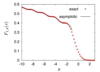
Figure 2: Plot of the exact edge density $F_{1,4}(s)$ as given in Eq. (4) (square symbols). The solid line corresponds to the asymptotic behaviour for $s\to-\infty$ given in Eq. (43).

It establishes the smooth matching for the density between the negative $s$ side of the edge scaling regime and the bulk regime. In Fig. (2) we show that this asymptotic behaviour (43) describes very accurately the oscillating behaviour of $F_{1,4}(s)$ for large negative $s$. Note finally that a similar matching with the bulk density is expected for all $n$ with

$$F_{1,2n}(s)\simeq\frac{1}{\pi}|s|^{\frac{1}{2n}}\;.$$ (44)

Of course, for arbitrary $n$, one also expects a (subleading) oscillating behaviour, as in Eq. (43).

C. Derivation of the scaling form of the kernel near the edge

Let us give a simple argument to establish the scaling form of the kernel near the edge (21). The energy eigenfunctions near the edge can be written more precisely as (16)

$$\hat{\psi}_{k}(p)\simeq c_{k}\operatorname{Ai}_{2n+1}\left(\frac{p-p_{e}}{p_{N}}+\frac{m(\mu-\epsilon_{k})}{p_{e}p_{N}}\right)\;.$$ (45)

where $c_{k}$ is an unknown coefficient which can be fixed e.g. using WKB approximation Eis2013 . Alternatively one can proceed as follows using the self-reproducibility property of the kernel. Inserting (45) into the kernel $K_{\mu}$, one finds that it takes the following form for $p,p^{\prime}$ near the edge

$$K_{\mu}(p,p^{\prime})\simeq\sum_{k}|c_{k}|^{2}\operatorname{Ai}_{2n+1}\left(\frac{p-p_{e}}{p_{N}}+\frac{m(\mu-\epsilon_{k})}{p_{e}p_{N}}\right)\operatorname{Ai}_{2n+1}\left(\frac{p^{\prime}-p_{e}}{p_{N}}+\frac{m(\mu-\epsilon_{k})}{p_{e}p_{N}}\right)\;.$$ (46)

which can be checked to decay rapidly to zero if $|p-p^{\prime}|\gg p_{N}$. In the large $\mu$ limit one can replace the sums over the eigenstates by an integral and defining $u=\frac{m(\mu-\epsilon_{k})}{p_{e}p_{N}}$, (46) takes the form

$$K_{\mu}(p,p^{\prime})\simeq\int du\,c(u)\operatorname{Ai}_{2n+1}(\frac{p-p_{e}}{p_{N}}+u)\operatorname{Ai}_{2n+1}(\frac{p^{\prime}-p_{e}}{p_{N}}+u)$$ (47)

where $\sum_{k}|c_{k}|^{2}$ has been replaced by $\int duc(u)$ with an unknown positive function $c(u)$ related to the coefficients $c_{k}$. Since $K_{\mu}(p,p^{\prime})$ is self-reproducing one has

$$\int dp^{\prime\prime}K_{\mu}(p,p^{\prime\prime})K_{\mu}(p^{\prime\prime},p^{\prime})=K_{\mu}(p,p^{\prime})$$ (48)

When $p,p^{\prime}$ are both near the edge, the integral over $p^{\prime\prime}$ is dominated by $p^{\prime\prime}$ close to the edge and one can thus use the scaling form (47). Using the orthonormality of the functions $\operatorname{Ai}_{2n+1}$, see (31), we see that it implies $p_{N}c(u)^{2}=c(u)$, hence $c(u)=1/p_{N}$ which demonstrates (21).

D. Some properties of the kernel $K_{\operatorname{Ai},2n+1}$

Here we derive some useful properties of the kernel mentioned in the text.

Self-reproducing property. As a consequence of the orthonormality of the $\operatorname{Ai}_{2n+1}$ functions, see (31), the kernel

$$K_{\operatorname{Ai},2n+1}(s,s^{\prime})=\int_{0}^{+\infty}du\operatorname{Ai}_{2n+1}(s+u)\operatorname{Ai}_{2n+1}(s^{\prime}+u)$$ (49)

is self-reproducing, since

$$\int_{-\infty}^{+\infty}ds^{\prime\prime}K_{\operatorname{Ai},2n+1}(s,s^{\prime\prime})K_{\operatorname{Ai},2n+1}(s^{\prime\prime},s^{\prime})$$ (50)

$$=\int_{0}^{+\infty}du_{1}\int_{0}^{+\infty}du_{2}\int_{-\infty}^{+\infty}ds^{\prime\prime}\operatorname{Ai}_{2n+1}(s+u_{1})\operatorname{Ai}_{2n+1}(s^{\prime\prime}+u_{1})\operatorname{Ai}_{2n+1}(s^{\prime\prime}+u_{2})\operatorname{Ai}_{2n+1}(s^{\prime}+u_{2})=K_{\operatorname{Ai},2n+1}(s,s^{\prime})$$

where we have used the orthonormality property (31) of the $\operatorname{Ai}_{2n+1}$ functions.

Differential equation for the kernel. From the definition of the kernel of sees that it satisfies the following differential equation

$$(\partial_{s}+\partial_{s^{\prime}})K_{\operatorname{Ai},2n+1}(s,s^{\prime})=\int_{0}^{+\infty}du\partial_{u}[\operatorname{Ai}_{2n+1}(s+u)\operatorname{Ai}_{2n+1}(s^{\prime}+u)]=-\operatorname{Ai}_{2n+1}(s)\operatorname{Ai}_{2n+1}(s^{\prime})$$ (51)

after integration since the function $\lim_{x\to+\infty}\operatorname{Ai}_{2n+1}(x)=0$. This generalises the identity for the Airy kernel $n=1$.

Christoffel-Darboux type formula. It is possible to express, for arbitrary $n$, the kernel directly in terms of the functions $\operatorname{Ai}_{2n+1}$. Let us first note the following identity, for any smooth function $f$ and integer $n\geq 1$

$$\partial_{u}\sum_{p=0}^{n-1}(-1)^{p}\left(f^{(p)}(s+u)f^{(2n-1-p)}(s^{\prime}+u)-f^{(p)}(s^{\prime}+u)f^{(2n-1-p)}(s+u)\right)=f(s+u)f^{(q)}(s^{\prime}+u)-f(s^{\prime}+u)f^{(q)}(s+u)$$ (52)

Hence we have, using this identity,

$$(s-s^{\prime})K_{\operatorname{Ai},2n+1}(s,s^{\prime})=\int_{0}^{+\infty}du(s+u-(s^{\prime}+u))\operatorname{Ai}_{2n+1}(s+u)\operatorname{Ai}_{2n+1}(s^{\prime}+u)$$ (53)

$$=(-1)^{n+1}\int_{0}^{+\infty}du\,\left[\operatorname{Ai}_{2n+1}^{(2n)}(s+u)\operatorname{Ai}_{2n+1}(s^{\prime}+u)-\operatorname{Ai}_{2n+1}(s+u)\operatorname{Ai}_{2n+1}^{(2n)}(s^{\prime}+u)\right]$$

$$=(-1)^{n}\int_{0}^{+\infty}du\partial_{u}\sum_{p=0}^{n-1}(-1)^{p}\left(\operatorname{Ai}_{2n+1}^{(p)}(s+u)\operatorname{Ai}_{2n+1}^{(2n-1-p)}(s^{\prime}+u)-\operatorname{Ai}_{2n+1}^{(p)}(s^{\prime}+u)\operatorname{Ai}_{2n+1}^{(2n-1-p)}(s+u)\right)$$

$$=(-1)^{n-1}\sum_{p=0}^{n-1}(-1)^{p}(\operatorname{Ai}_{2n+1}^{(p)}(s)\operatorname{Ai}_{2n+1}^{(2n-1-p)}(s^{\prime})-\operatorname{Ai}_{2n+1}^{(p)}(s^{\prime})\operatorname{Ai}_{2n+1}^{(2n-1-p)}(s))$$

Finally we obtain

$$K_{\operatorname{Ai},2n+1}(s,s^{\prime})=\frac{(-1)^{n-1}\sum_{p=0}^{n-1}(-1)^{p}(\operatorname{Ai}_{2n+1}^{(p)}(s)\operatorname{Ai}_{2n+1}^{(2n-1-p)}(s^{\prime})-\operatorname{Ai}_{2n+1}^{(p)}(s^{\prime})\operatorname{Ai}_{2n+1}^{(2n-1-p)}(s))}{s-s^{\prime}}$$ (54)

For $n=1$ we recover the standard formula for the Airy kernel

$$K_{\operatorname{Ai}}(s,s^{\prime})=\frac{1}{s-s^{\prime}}[\operatorname{Ai}(s)\operatorname{Ai}^{\prime}(s^{\prime})-\operatorname{Ai}^{\prime}(s)\operatorname{Ai}(s^{\prime})]$$ (55)

and for $n=2$ one obtains the formula (22) given in the text.

E. Finite temperature kernel

We give a short derivation of the finite $T$ form of the kernel given in the text, using the general method introduced in fermions_review which relates the finite $T$ kernel to the $T=0$ one. For simplicity we set here $m=\hbar=1$ and restore the units at the end. We consider the kernel in the grand canonical ensemble in momentum space, denoted $K_{\tilde{\mu},2n+1}$, at chemical potential $\tilde{\mu}$ (see fermions_review for definitions and details). We are interested in its form near the edge $p_{e}$. It can be obtained by inserting the zero temperature scaling form (21) into Eq. 240 of fermions_review , leading to

$$K_{\tilde{\mu},2n+1}(p,p^{\prime})\simeq\int d\mu^{\prime}\frac{1}{1+e^{\beta(\mu^{\prime}-\tilde{\mu})}}\partial_{\mu^{\prime}}\frac{1}{p_{N}(\mu^{\prime})}K_{\operatorname{Ai},2n+1}(\frac{p-p_{e}(\mu^{\prime})}{p_{N}(\mu^{\prime})},\frac{p^{\prime}-p_{e}(\mu^{\prime})}{p_{N}(\mu^{\prime})})$$ (56)

where $p,p^{\prime}$ are near the edge, $p_{e}(\mu^{\prime})=\sqrt{2\mu^{\prime}}$ and $p_{N}(\mu^{\prime})=(g/p_{e}(\mu^{\prime}))^{1/(2n+1)}$. We recall that near the edge $\tilde{\mu}\approx\mu$ fermions_review . Note that one can neglect the action of $\partial_{\mu}$ on the factor $1/p_{N}(\mu)$. One has

$$\frac{p-p_{e}(\mu^{\prime})}{p_{N}(\mu^{\prime})}=\frac{p-p_{e}(\mu)}{w_{N}(\mu)}-\beta_{\mu}(\mu^{\prime}-\mu)+O((\mu^{\prime}-\mu)^{2})$$ (57)

$$\beta_{\mu}=\frac{1}{p_{N}(\mu)}\partial_{\mu}p_{e}(\mu)=g^{-1/(2n+1)}p_{e}^{1/(2n+1)}\partial_{\mu}p_{e}(\mu)=g^{-1/(2n+1)}2^{-\frac{n}{2n+1}}\mu^{-\frac{n}{1+2n}}$$ (58)

the first term is subdominant. We define $\beta(\mu^{\prime}-\mu)=-bu$, hence

$$\frac{p-p_{e}(\mu^{\prime})}{p_{N}(\mu^{\prime})}=\frac{p-p_{e}(\mu)}{p_{N}(\mu)}+b\frac{\beta_{\mu}}{\beta}u+O((\mu^{\prime}-\mu)^{2})$$ (59)

This leads to the definition of the scaled inverse temperature $b$ as given in the text, Eq. (23) (restoring units), so that $b\frac{\beta_{\mu}}{\beta}=1$. Hence we find that the kernel takes the scaling form

$$K_{\mu,2n+1}(p,p^{\prime})\simeq-\frac{1}{p_{N}(\mu)}\int du\frac{1}{1+e^{-bu}}\partial_{u}K_{{\rm Ai},2n+1}(\frac{p-p_{e}(\mu)}{p_{N}(\mu)}+u,\frac{p^{\prime}-p_{e}(\mu)}{p_{N}(\mu)+u})$$ (60)

$$=\frac{1}{p_{N}(\mu)}\int_{-\infty}^{+\infty}du\frac{1}{1+e^{-bu}}{\rm Ai}_{2n+1}(\frac{p-p_{e}(\mu)}{p_{N}(\mu)}+u){\rm Ai}_{2n+1}(\frac{p^{\prime}-p_{e}(\mu)}{p_{N}(\mu)}+u)$$ (61)

$$=\frac{1}{p_{N}(\mu)}K_{2n+1,b}(\frac{p-p_{e}(\mu)}{p_{N}(\mu)},\frac{p^{\prime}-p_{e}(\mu)}{p_{N}(\mu)})$$ (62)

where $K_{2n+1,b}$ is given in the text in (24).

High temperature limit. Let us examine the high temperature limit of the edge regime, i.e. small $b=T^{*}/T\ll 1$. The following property is shown in AlexST . Consider any determinantal process $k_{i}\in\mathbb{R}$ characterised by a kernel $K(k,k^{\prime})$ of the form

$$K(k,k^{\prime})=\int du\frac{1}{1+e^{-bu}}f(k+u)f(k^{\prime}+u)$$ (63)

with a density $\rho_{K}(k)=K(k,k)$ which behaves at large negative $k$ as $\rho_{K}(k)\simeq_{k\to-\infty}A|k|^{\alpha}$. Then, it is shown in AlexST that, in the limit of small $b$, the CDF of the variable $\xi=bk$ takes the large deviation form

$${\rm Prob}(\xi<r)\sim\exp(-b^{-\frac{1+\alpha}{\alpha}}\Psi(e^{-r}))\quad,\quad\Psi(z):=A\int_{-\infty}^{0}da|a|^{\alpha}\ln(1+ze^{a})$$ (64)

For the present application we will set $\alpha=1/(2n)$, $A=1/\pi$ and $K=K_{\operatorname{Ai},2n+1}$, $f=\operatorname{Ai}_{2n+1}$, and consider the determinantal process $k_{i}=\frac{p_{i}(T)-p_{e}}{p_{N}}$, where the $p_{i}$ are the momenta of the fermions in the grand canonical ensemble at temperature $T$. Introducing the scaled variable

$$\xi=bk=b\frac{p_{i}(T)-p_{e}}{p_{N}}$$ (65)

we find, from the above result, that for small $b\ll 1$

$${\rm Prob}(\xi<r)=\exp(-b^{-\frac{2n+1}{2n}}\Psi_{2n}(e^{-r}))\quad,\quad\Psi_{2n}(z)=-\frac{1}{\pi}\Gamma(1+\frac{1}{2n}){\rm Li}_{2+\frac{1}{2n}}(-z)$$ (66)

This is a generalisation, for arbitrary $n$, of the result of UsShortTime for $n=1$. Hence in the regime of typical fluctuations, expanding $\Psi_{2n}(z)$ to $O(z)$, we find that

$${\rm Prob}(\xi<r)=\exp(-b^{-\frac{2n+1}{2n}}\frac{1}{\pi}\Gamma(1+\frac{1}{2n})e^{-r})$$ (67)

Hence the typical value of $\xi$ is $\xi_{typ}=\ln(b^{-\frac{2n+1}{2n}}\frac{1}{\pi}\Gamma(1+\frac{1}{2n}))$, and the typical fluctuations are of Gumbel type, i.e. one has $\xi=\xi_{typ}+G$ where $G$ is a unit Gumbel random variable. In particular the variance is

$${\rm Var}[b\frac{p_{\rm max}(T)-p_{e}}{p_{N}}]=\frac{\pi^{2}}{6}$$ (68)

as given in the text, below Eq. (24).

F. Painlevé II hierarchy and asymptotics of the Fredholm determinant ${\cal F}_{2n}$

Painlevé II hierarchy. Let us recall here the definition of the Painlevé II hierarchy of non linear differential equations. We follow e.g. Eqs. (1.31-1.32) of Ref. Claes1 (and see references therein). The $n$-th member of the Painlevé II hierarchy is a differential equation for the function $g(x)$, which reads (for the special case $\tau_{i}=\alpha_{i}=0$ which is relevant here)

$$(\partial_{x}+2g)L_{n}[g^{\prime}-g^{2}]=xg$$ (69)

where the $L_{j}$ are operators which transform a function into a function and are defined recursively as

$$\partial_{x}L_{j+1}f=(\partial_{x}^{3}+4f\partial_{x}+2f^{\prime})L_{j}f\quad,\quad L_{0}f=\frac{1}{2}$$ (70)

For $n=1$, one finds $L_{1}f=f$ and the standard Painlevé II equation

$$g^{\prime\prime}(x)=xg(x)+2g(x)^{3}$$ (71)

given in the text for the function denoted there $q(s)=g(s)$. Next, for $n=2$ one finds $L_{2}f=f^{\prime\prime}+3f^{2}$ and

$$g^{\prime\prime\prime\prime}(x)=xg(x)+10g(x)g^{\prime}(x)^{2}+10g(x)^{2}g^{\prime\prime}(x)-6g(x)^{5}$$ (72)

which leads to (11) in the text, for the function $q(s)=g(-s)$. More generally the function $q(s)$ defined in the text for arbitrary $n$ is given by $q(s)=g((-1)^{n+1}s)$.

Asymptotics of the Fredholm determinant ${\cal F}_{2n}$. Let us study the behaviour of $q(s)=g((-1)^{n+1}s)$ for $s\to-\infty$. Examination shows that in the equations (71) and (72) one can neglect all derivatives, to leading order for large negative $s$ (with $x=(-1)^{n+1}s$). Going back to the recursion relation of the PII hierarchy (69) these simplified equations can be obtained more systematically by performing the same approximation, leading to the simplified recursion

$$2gL_{n}[-g^{2}]=xg\quad,\quad\partial_{x}L_{j+1}f=(4f\partial_{x}+2f^{\prime})L_{j}f\quad,\quad L_{0}f=\frac{1}{2}$$ (73)

The second equation is solved by writing $L_{j}f=a_{j}f^{j}$ and leads to the recursion relation $(j+1)a_{j+1}=4(j+\frac{1}{2})a_{j}$ with $a_{0}=\frac{1}{2}$, hence

$$a_{j}=2^{2j-1}\frac{\Gamma(j+\frac{1}{2})}{\sqrt{\pi}\Gamma(j+1)}$$ (74)

with $a_{0}=1/2$, $a_{1}=1$, $a_{2}=3$. It finally leads to

$$q(s)\simeq\kappa_{n}(-s)^{\frac{1}{2n}}\quad,\quad\kappa_{n}=\frac{1}{2}[\frac{\sqrt{\pi}\Gamma(n+1)}{\Gamma(n+\frac{1}{2})}]^{\frac{1}{2n}}$$ (75)

We now recall that the Fredholm determinant (9) is obtained from the function $q(s)$, solution of the Painlevé equation $P_{\rm II}^{(n)}$ with the boundary condition $q(s)\sim_{s\to+\infty}\operatorname{Ai}_{2n+1}(s)$, through the formula (10) (see derivation in Section G)

$$\ln{\cal F}_{2}(s)=-\int_{s}^{+\infty}du(u-s)q(u)^{2}$$ (76)

Plugging in (75), this leads to the result given in the text below Eq. (11) for $s\to-\infty$

$$\ln{\cal F}_{2n}(s)\simeq-f_{n}(-s)^{2+\frac{1}{n}}\quad,\quad f_{n}=\frac{n^{2}}{4(2n+1)(n+1)}[\frac{\sqrt{\pi}\Gamma(n+1)}{\Gamma(n+\frac{1}{2})}]^{\frac{1}{n}}$$ (77)

For $n=2$ we find, explicitly

$$q(s)\simeq\frac{1}{6^{1/4}}|s|^{1/4}-\frac{5}{16\ 6^{3/4}|s|^{9/4}}-\frac{99\ 3^{3/4}}{512\sqrt[4]{2}|s|^{19/4}}+..\quad,\quad\ln{\cal F}_{4}(s)\simeq-\frac{2\sqrt{2}}{15\sqrt{3}}(-s)^{5/2}+O(s)$$ (78)

This asymptotics for ${\cal F}_{4}(s)$ is plotted in Fig. 1.

G. Differential equation for the Fredholm determinant ${\cal F}_{2n}$ and the connection to the second Painlevé hierarchy

In this section we obtain the differential equation satisfied by the Fredholm determinant ${\cal F}_{2n}$ in Eq. (9) of the text. To this aim we first define the problem in a more general framework. We consider the following Fredholm determinant

$$F(s):={\rm Det}(I-\hat{K})\quad,\quad\hat{K}=KP_{s}\Leftrightarrow\hat{K}(x,y)=K(x,y)\theta(y-s)$$ (79)

where $K$ is a kernel which satisfies the following three properties:

• property 1: The kernel can be constructed from a function $\phi(x)$ and its derivatives as

  $$K(x,y)=\langle x|K|y\rangle=\frac{1}{x-y}\left((-1)^{n-1}\sum_{p=0}^{n-1}(-1)^{p}(\langle x|\phi^{(p)}\rangle\langle\phi^{(2n-1-p)}|y\rangle-\langle x|\phi^{(2n-1-p)}\rangle\langle\phi^{(p)}|y\rangle\right)$$ (80)

  in quantum mechanical notations, where $|\phi\rangle=|\phi^{(0)}\rangle$ is the ket (vector) associated to the function $\langle x|\phi\rangle=\phi(x)$ and $|\phi^{(p)}\rangle$ denote the kets associated to the derivatives $\langle x|\phi^{(p)}\rangle=\phi^{(p)}(x)$.

• property 2: The kernel satisfies

  $$(\partial_{x}+\partial_{y})K(x,y)=-\phi(x)\phi(y)$$ (81)

• property 3: The function $\phi(x)$ obeys the differential equation

  $$\phi^{(2n)}(x)=(-1)^{n+1}\phi(x)$$ (82)

One recognises that $\phi(x)=\operatorname{Ai}_{2n+1}(x)$ and $K=K_{\operatorname{Ai},2n+1}$ defined in the text satisfy these three properties, with $F(s)={\cal F}_{2n}(s)$. The first is the Christoffel-Darboux property (54), the second is (51) and the third is (30). Whenever these three properties hold, a closed system of differential equations can be derived for the Fredholm determinant. Here we follow and extend the derivation of Tracy and Widom in TracyWidomAiry who treated the case $n=1$ (Airy kernel). A similar, but somewhat different, extension was obtained by Brézin and Hikami in BrezinHikamiSource , to which we also refer. We first derive the equations, and in a second part we analyse them and relate them to the second Painlevé hierarchy.

Derivation of the differential equations. We start by applying $\partial_{s}$ to the logarithm of (79) which leads to

$$\partial_{s}\ln F(s)=\partial_{s}{\rm Tr}\ln(I-\hat{K})=-{\rm Tr}(1-\hat{K})^{-1}\partial_{s}\hat{K}={\rm Tr}(1-\hat{K})^{-1}K|s\rangle\langle s|=\tilde{K}(s,s)\quad,\quad\tilde{K}=\frac{\hat{K}}{1-\hat{K}}$$ (83)

which is simply the diagonal element of the operator $\tilde{K}$. We have used the expression for the derivative

$$\partial_{s}\hat{K}(x,y)=-K(x,y)\delta(y-s)\Leftrightarrow\partial_{s}\hat{K}=-K|s\rangle\langle s|$$ (84)

where we recall that $\langle x|y\rangle=\delta(x-y)$. We now derive a differential equation satisfied by $\tilde{K}(s,s)$. The route is an extension of TracyWidomAiry and requires introducing two sets of $2n$ auxiliary functions. Before doing so, let us define the two operators, the position $X$, and the derivative $D$, as follows. For any $x,y$ and ket vector $|f\rangle$

$$\langle x|D|f\rangle=f^{\prime}(x)=-\langle f|D|x\rangle\quad,\quad\langle x|X=x\langle x|\quad,\quad X|y\rangle=y|y\rangle$$ (85)

where $\langle x|f\rangle=f(x)$. To manipulate them, we need to recall the operator commutator and derivation identities TracyWidomAiry

$$[L,(1-\hat{K})^{-1}]=(1-\hat{K})^{-1}[L,\hat{K}](1-\hat{K})^{-1}\quad,\quad\partial(1-\hat{K})^{-1}=(1-\hat{K})^{-1}\partial\hat{K}(1-\hat{K})^{-1}$$ (86)

which we will use repeatedly for $L=D$ or $L=X$.

Let us now use property 1, i.e. Eq. (80). Since $\langle x[X,K]|y\rangle=(x-y)K(x,y)$ we obtain, upon further right multiplication by $P_{s}$ (using that $X$ and $P_{s}$ commute)

$$[X,\hat{K}]=(-1)^{n-1}\sum_{p=0}^{n-1}(-1)^{p}(|\phi^{(p)}\rangle\langle\phi^{(2n-1-p)}|-|\phi^{(2n-1-p)}\rangle\langle\phi^{(p)}|)P_{s}$$ (87)

Hence, using that $\tilde{K}=(I-\hat{K})^{-1}-I$,

$$(x-y)\tilde{K}(x,y)=\langle x|[X,\tilde{K}]|y\rangle=\langle x|(1-\hat{K})^{-1}[X,\hat{K}](1-\hat{K})^{-1}|y\rangle$$ (88)

$$=(-1)^{n-1}\sum_{p=0}^{n-1}(-1)^{p}\langle x|(1-\hat{K})^{-1}(|\phi^{(p)}\rangle\langle\phi^{(2n-1-p)}|-|\phi^{(2n-1-p)}\rangle\langle\phi^{(p)}|)P_{s}(1-\hat{K})^{-1}|y\rangle$$ (89)

$$=(-1)^{n-1}\sum_{p=0}^{n-1}(-1)^{p}[q_{p}(s;x)\tilde{q}_{2n-1-p}(s;y)-q_{2n-1-p}(s;x)\tilde{q}_{p}(s;y)]$$ (90)

where we have defined the $2n$ auxiliary functions, for $p=0,..2n-1$

$$q_{p}(s;x):=\langle x|(1-\hat{K})^{-1}|\phi^{(p)}\rangle=\phi^{(p)}(x)+\int_{y>s}K(x,y)\phi^{(p)}(y)+\int_{y_{1}>s,y_{2}>s}K(x,y_{1})K(y_{1},y_{2})\phi^{(p)}(y_{2})+\cdots$$ (91)

$$\tilde{q}_{p}(s;x):=\langle\phi^{(p)}|P_{s}(1-\hat{K})^{-1}|x\rangle=\theta(y-s)[\phi^{(p)}(y)+\int_{x>s}\phi^{(p)}(x)K(x,y)+\int_{x_{1}>s,x_{2}>s}\phi^{(p)}(x_{1})K(x_{1},x_{2})K(x_{2},y)+\cdots]$$

Note that $q_{p}(s;x)$ is smooth, while $\tilde{q}_{p}(s;x)$ is not smooth (it vanishes for $x<s$), and in fact one has $\tilde{q}_{p}(s;y)=q_{p}(s;y)\theta(y-s)$. Hence in the following we only need $n$ auxiliary functions $q_{p}$. This leads to (for $y\to s^{+}$, the same limit procedure as in TracyWidomAiry )

$$\tilde{K}(s,s)=(-1)^{n-1}\sum_{p=0}^{n-1}(-1)^{p}[\partial_{x}q_{p}(s;x)|_{x=s}q_{2n-1-p}(s;s)-\partial_{x}q_{2n-1-p}(s;x)|_{x=s}q_{p}(s;s)]$$ (92)

We now establish a set of differential equations for the functions $q_{p}(s;x)$. It then leads to establishing two closed sets of $2n$ differential equations (each) for $q_{p}(s)$ and $u_{p}(s)$, respectively, $p=0,\cdots 2n-1$, defined as

$$q_{p}(s):=q_{p}(s;s)=\langle x|(1-\hat{K})^{-1}|\phi^{(p)}\rangle\quad,\quad u_{p}(s):=\langle\phi|P_{s}(1-\hat{K})^{-1}|\phi^{(p)}\rangle$$ (93)

The first set of differential equations reads (in two parts)

$$\partial_{x}q_{p}(s;x)=q_{p+1}(s;x)-q_{0}(s;x)u_{p}(s)+\tilde{K}(x,s)q_{p}(s)\quad,\quad\partial_{s}q_{p}(s)=q_{p+1}(s)-q_{0}(s)u_{p}(s)$$ (94)

To obtain it we use property 2, i.e. Eq. (81). It allows to establish that

$$[D,\hat{K}]=-|\phi\rangle\langle\phi|P_{s}+K|s\rangle\langle s|$$ (95)

Indeed one has

$$\langle x|[D,\hat{K}]|y\rangle=\partial_{x}(K(x,y)\theta(y-s))+\partial_{y}(K(x,y)\theta(y-s))=[(\partial_{x}+\partial_{y})K(x,y)]\theta(y-s)+\langle x|K|s\rangle\langle s|y\rangle$$ (96)

Using property 2, i.e. Eq. (81), this leads to (95).

Using (86) and (95) we now calculate the derivative

$$\partial_{x}q_{p}(s;x)=\langle x|D(1-\hat{K})^{-1}|\phi^{(p)}\rangle=q_{p+1}(s;x)+\langle x|[D,(1-\hat{K})^{-1}]|\phi^{(p)}\rangle$$ (97)

$$=q_{p+1}(s;x)+\langle x|(1-\hat{K})^{-1}[D,\hat{K}](1-\hat{K})^{-1}|\phi^{(p)}\rangle=q_{p+1}(s;x)+\langle x|(1-\hat{K})^{-1}[-|\phi\rangle\langle\phi|P_{s}+K|s\rangle\langle s|](1-\hat{K})^{-1}|\phi^{(p)}\rangle$$

$$=q_{p+1}(s;x)-q_{0}(s;x)\langle\phi|P_{s}(1-\hat{K})^{-1}|\phi^{(p)}\rangle+\tilde{K}(x,s)q_{p}(s;s)$$

which establishes, using the definition (93), the first part of (94). We have used that $P_{s}|s\rangle=|s\rangle$ which implies that $\tilde{K}(x,s)=\langle x|(1-\hat{K})^{-1}K|s\rangle=\langle x|(1-\hat{K})^{-1}\hat{K}|s\rangle$. The second part of (94) is established in the same way. We calculate the total derivative with respect to $s$

$$\partial_{s}q_{p}(s;s)=\langle s|D(1-\hat{K})^{-1}|\phi^{(p)}\rangle+\langle s|(1-\hat{K})^{-1}\partial_{s}\hat{K}(1-\hat{K})^{-1}|\phi^{(p)}\rangle$$ (98)

Hence it is similar to (97) except that there is an additional term

$$\langle s|(1-\hat{K})^{-1}\partial_{s}\hat{K}(1-\hat{K})^{-1}|\phi^{(p)}\rangle=-\langle s|(1-\hat{K})^{-1}K|s\rangle\langle s|(1-\hat{K})^{-1}|\phi^{(p)}\rangle=-\tilde{K}(s,s)q_{p}(s;s)$$ (99)

which simply cancels the term $\tilde{K}(s,s)q_{p}(s)$ in the first part of (94) and leads to the second part of (94).

We now establish the differential equations for the second set of auxiliary functions, $u_{p}(s)$. We first calculate

$$\partial_{s}[P_{s}(1-\hat{K})^{-1}]=-(|s\rangle+P_{s}(1-\hat{K})^{-1}K|s\rangle)\langle s|(1-\hat{K})^{-1}$$ (100)

$$=-(P_{s}+P_{s}(1-\hat{K})^{-1}\hat{K}|s\rangle)\langle s|(1-\hat{K})^{-1}=-P_{s}(1-\hat{K})^{-1}|s\rangle\langle s|(1-\hat{K})^{-1}$$ (101)

where we used again that $P_{s}|s\rangle=|s\rangle$. Hence

$$\partial_{s}u_{p}(s)=\langle\phi|(\partial_{s}[P_{s}(1-\hat{K})^{-1}])|\phi^{(p)}\rangle=-\langle\phi|P_{s}(1-\hat{K})^{-1}|s\rangle\langle s|(1-\hat{K})^{-1}|\phi^{(p)}\rangle$$ (102)

$$=-\tilde{q}_{0}(s,s)q_{p}(s)=-q_{0}(s)q_{p}(s)$$ (103)

since $\tilde{q}_{0}(s,s)=\tilde{q}_{0}(s^{+},s)=q_{0}(s)$.

Since (94) relates $q_{p}$ and $q_{p+1}$ we still need to close the equations. Fortunately one can now use the property 3, i.e. Eq. (82), which can also be written as $|\phi^{(2n)}\rangle=(-1)^{n+1}X|\phi\rangle$. It allows to express $q_{2n}$ in terms of the $q_{p}$, and $u_{p}$, for $p=0,..2n-1$, hence it closes the equations. One has

$$q_{2n}(s;x)=\langle x|(1-\hat{K})^{-1}|\phi^{(2n)}\rangle=(-1)^{n+1}\langle x|(1-\hat{K})^{-1}X|\phi\rangle=(-1)^{n+1}(xq_{0}(s;x)+\langle x|[(1-\hat{K})^{-1},X]|\phi\rangle)$$ (104)

$$=(-1)^{n+1}(xq_{0}(s;x)-\langle x|(1-\hat{K})^{-1}[X,\hat{K}](1-\hat{K})^{-1}|\phi\rangle)$$ (105)

$$=(-1)^{n+1}xq_{0}(s;x)-\big{(}\langle x|(1-\hat{K})^{-1}[\sum_{p=0}^{n-1}(-1)^{p}(|\phi^{(p)}\rangle\langle\phi^{(2n-1-p)}|-|\phi^{(2n-1-p)}\rangle\langle\phi^{(p)}|)]P_{s}(1-\hat{K})^{-1}|\phi\rangle\big{)}$$ (106)

$$=(-1)^{n+1}xq_{0}(s;x)-\sum_{p=0}^{n-1}(-1)^{p}(q_{p}(s;x)u_{2n-1-p}(s)-q_{2n-1-p}(s;x)u_{p}(s))$$ (107)

We use this equation for $x=s$. We have used that $P_{s}(1-\hat{K})^{-1}=P_{s}+P_{s}KP_{s}+P_{s}KP_{s}KP_{s}+\cdots$ is a symmetric operator, hence $\langle\phi^{(p)}|P_{s}(1-\hat{K})^{-1}|\phi\rangle=\langle\phi|P_{s}(1-\hat{K})^{-1}|\phi^{(p)}\rangle=u_{p}(s)$.

Finally, we can go back to the equation (92) and perform the derivatives using the equations (94). It leads to

$$\tilde{K}(s,s)=(-1)^{n-1}\sum_{p=0}^{n-1}(-1)^{p}[q^{\prime}_{p}(s)q_{q-1-p}(s)-q^{\prime}_{q-1-p}(s)q_{p}(s)]$$ (108)

Summary of the equations. Let us now recapitulate the system of equations obtained above for any fixed integer $n$. The $4n$ functions $\{q_{p}(s),u_{p}(s)\}_{0\leq p\leq 2n-1}$ satisfy the closed system

$$q_{p}^{\prime}=q_{p+1}-q_{0}u_{p}\quad,\quad u_{p}^{\prime}=-q_{0}q_{p}\quad,\quad 0\leq p\leq 2n-1$$ (109)

where, in addition

$$q_{2n}=(-1)^{n+1}sq_{0}-\sum_{p=0}^{n-1}(-1)^{p}(q_{p}u_{2n-1-p}-q_{2n-1-p}u_{p})$$ (110)

From their definitions $\{q_{p}(s),u_{p}(s)\}_{0\leq p\leq 2n-1}$ in (93), they vanish for $s\to+\infty$. This system allows to calculate $\tilde{K}(s,s)$ from

$$\tilde{K}(s,s)=(-1)^{n-1}\sum_{p=0}^{n-1}(-1)^{p}[q^{\prime}_{p}(s)q_{q-1-p}(s)-q^{\prime}_{q-1-p}(s)q_{p}(s)]$$ (111)

Remarkably, using the above equations one can check that

$$\partial_{s}\tilde{K}(s,s)=-q_{0}(s)^{2}$$ (112)

Hence, to summarise, the Fredholm determinant satisfies

$$\partial_{s}^{2}\ln F(s)=-q_{0}(s)^{2}$$ (113)

where $q_{0}(s)$ is determined from the system (109), (110). Note that this equation (113) corresponds to (10) in the text, where we denote $q_{0}(s)=q(s)$.

For $n=1$ it is interesting to compare with the results of Tracy and Widom. One recovers the equations (1.6-1.9) of TracyWidomAiry : one must consider $j=1$ there, i.e. remove the index $j$ everywhere and discard the terms $\sum_{k\neq j}$, with $a_{j}=a=s$, $u_{0}=u$, $u_{1}=v$, $q_{0}=q$ and $q_{1}=p$. Eq. (110) here is then the same as (1.10) there, and Eq. (111) the same as (2.8-2.10) there. Finally (113) is (1.14) there.

Analysis of the equations: Painlevé II hierarchy. We now analyse the equations (109), (110), (113) and establish the connection to the Painlevé II hierarchy, as discussed in the text. We find that the function $q_{0}(s)$, which is denoted $q(s)$ in the text, satisfies a closed differential equation, which coincides with the $n$-th member of the Painlevé II hierarchy. The latter is recalled in section F.

To analyse the flow, it is useful to identify invariants. We find that there are $n$ quadratic invariants $I_{p}$, $1\leq p\leq n$,

$$I_{p}=u_{2p-1}+\frac{1}{2}\sum_{k=0}^{2p-2}(-1)^{k+1}(u_{k}u_{2p-2-k}-q_{k}q_{2p-2-k})=0$$ (114)

Note that they do not depend explicitly on $n$, i.e. the invariants for $n^{\prime}<n$ are a subset of those for $n$. It is immediate to check that

$$\partial_{s}I_{p}=-q_{0}q_{2p-1}-\frac{1}{2}\sum_{k=0}^{2p-2}(-1)^{k+1}(q_{k+1}q_{2p-2-k}+q_{k}q_{2p-1-k})=0$$ (115)

using that the sum is telescopic of the form $\sum_{k=0}^{2p-2}(-1)^{k+1}(Q_{k}+Q_{k+1})=-Q_{0}-Q_{2p-1}$ with $Q_{k}=q_{k}q_{2p-1-k}$. Furthermore since all the functions vanish at $s\to+\infty$ along the flow the invariants exactly vanish $I_{p}(s)=0$.

Remarkably, using these invariants, it is possible to eliminate all functions apart from $q_{0}$, and write a closed equation for $q_{0}$. Using the condition that the invariants vanish, $I_{p}=0$, $p=1,..n$, we express the odd $u_{2k+1}(s)$ as a function of all other functions. Then it is possible to obtain recursively all $q_{p}$ for $1\leq p\leq 2n-2$ only in terms of $q_{0}$ and its derivatives and of the even $u_{2k}(s)$ (not their derivatives). Finally one calculates the $2n$-th derivative of $q_{0}$, $q_{0}^{(2n)}$, using (109) and (110) as well as these substitutions. All dependence in the $u_{2k}(s)$ then cancels.

For $n=1$, from (109) we have $q^{\prime\prime}_{0}=q_{1}^{\prime}-(q_{0}u_{0})^{\prime}=q_{1}^{\prime}-q_{0}^{\prime}u_{0}+q_{0}^{3}$, and using $q_{1}^{\prime}=q_{2}-q_{0}u_{1}=sq_{0}+q_{1}u_{0}-2q_{0}u_{1}$ from (110), we obtain $q_{0}^{\prime\prime}=sq_{0}+q_{1}u_{0}-2q_{0}u_{1}-q_{0}^{\prime}u_{0}+q_{0}^{3}$. Using that $q_{1}=q_{0}^{\prime}+q_{0}u_{0}$ and replacing $u_{1}$ using the invariant $I_{1}=u_{1}+\frac{1}{2}(u_{0}^{2}-q_{0}^{2})=0$ we see that $u_{0}$ cancels and we are left with $q_{0}^{\prime\prime}=sq_{0}+2q_{0}^{3}$, the usual Painlevé II equation.

For $n=2$ the same procedure yields, after a tedious calculation, the following equation for $q_{0}$ (as given in the text, Eq. (11) with $q_{0}=q$)

$$q_{0}^{\prime\prime\prime\prime}=q_{0}\left(10(q_{0}^{\prime})^{2}+10q_{0}q_{0}^{\prime\prime}-6q_{0}^{4}-s\right)$$ (116)

which is exactly (up to a change of sign of the argument) $P_{\rm II}^{(2)}$ a particular case of the second member of the second Painlevé hierarchy, as discussed in Section F.

We now conjecture, as announced in the text, that this property, i.e. $q_{0}(s)=g((-1)^{n+1}s)$ where $g(x)$ is the solution of the $n$-th member of the second Painlevé hierarchy, recalled in Section F, hold for arbitrary $n$. We have checked this conjecture with Mathematica, using the above differential system, up to large values of $n$.

Hamiltonian structure of the differential system. It is interesting to point out another remarkable property of the above system of differential equations (109), (110). Indeed, for $n=1$ it is known that there is a Hamiltonian structure underlying the Painlevé II equation, see TracyWidomAiry and references therein. Here also, we find a Hamiltonian structure, which is quite simple. The Hamiltonian reads

$$H[q,u]=(-1)^{n}\frac{1}{2}sq_{0}^{2}+\frac{1}{2}\sum_{p=1}^{2n-1}(-1)^{p+1}q_{p}q_{2n-p}+q_{0}\sum_{p=0}^{2n-1}(-1)^{p+1}u_{p}q_{2n-1-p}$$ (117)

Then one can check that the equations (109), (110) can be written as

$$q^{\prime}_{p}=(-1)^{p}\frac{\partial H[q,u]}{\partial q_{2n-1-p}}\quad,\quad u^{\prime}_{p}=(-1)^{p+1}\frac{\partial H[q,u]}{\partial u_{2n-1-p}}\quad,\quad p=0,\cdots,2n-1$$ (118)

Note that

$$\frac{dH}{ds}=\frac{\partial H}{\partial s}=\frac{1}{2}q_{0}^{2}=-\frac{1}{2}u_{0}^{\prime}$$ (119)

Hence $\tilde{H}=H+\frac{u_{0}}{2}$ is an additional invariant of motion, which is cubic. Comparing with (112) we see that

$$-H[q(s),u(s)]=\tilde{K}(s,s)$$ (120)

since both vanish for $s\to+\infty$, related to the derivative of the logarithm of the Fredholm determinant ${\cal F}_{2n}$ through Eq. (83). Finally we note that for the Painlevé II hierarchy there exists a Hamiltonian formulation Mo-Hamiltonian , which however looks much more complicated. A route to prove our conjecture would be to establish the equivalence between the two Hamiltonian dynamics. It is worth pointing out that, as a byproduct of our work, we have found a simple Hamiltonian structure for arbitrary $n$.

References

(1)
S. Giorgini, L. P. Pitaevski, S. Stringari, Rev. Mod. Phys. 80, 1215 (2008).
(2)
I. Bloch, J. Dalibard, W. Zwerger, Rev. Mod. Phys. 80, 885 (2008).
(3)Y. Castin, in Ultra-cold Fermi Gases, ed. by
M. Inguscio, W. Ketterle, and C. Salomon, (2006), see also arXiv:0612613.
(4)
W. Kohn, A. E. Mattsson, Phys. Rev. Lett. 81 3487 (1998).
(5)
V. Eisler, Phys. Rev. Lett. 111, 080402 (2013).
(6)
D. S. Dean, P. Le Doussal, S. N. Majumdar, G. Schehr, Phys. Rev. Lett. 114, 110402 (2015).
(7)
D. S. Dean, P. Le Doussal, S. N. Majumdar, G. Schehr, Europhys. Lett. 112, 60001 (2015)
(8)
D. S. Dean, P. Le Doussal, S. N. Majumdar, G. Schehr, Phys. Rev. A 94, 063622 (2016).
(9)
N. Allegra, J. Dubail, J.-M. Stéphan, J. Viti,
J. Stat. Mech. (2016) 053108
(10)
C. Chin et al.,
Rev. Mod. Phys., 82, 1225 (2010).
(11)
K. Hueck et al., Phys. Rev. Lett. 120, 060402 (2018).
(12)
L. W. Cheuk, M. A. Nichols, M. Okan, T. Gersdorf, R.Vinay, W. Bakr, T. Lompe, M. Zwierlein, Phys. Rev. Lett. 114, 193001, (2015).
(13)
E. Haller, J. Hudson, A. Kelly, D. A. Cotta, B. Peaudecerf, G. D. Bruce, S. Kuhr, Nature Physics 11, 738 (2015).
(14)
M. F. Parsons, F. Huber, A. Mazurenko, C. S. Chiu, W. Setiawan, K. Wooley-Brown, S. Blatt, M. Greiner, Phys. Rev. Lett. 114, 213002 (2015).
(15)
A. Omran et al.,
Phys. Rev. Lett. 115, 263001 (2015).
(16)
see e.g. Proc. of International School of Physics ”Enrico Fermi”, Ultracold Fermi gases, Course CLXIV, Varenna, IT, M. Inguscio, W. Ketterle, and C. Salomon eds. IOS, June (2008).
(17)
R. Marino, S. N. Majumdar, G. Schehr, P. Vivo, Phys. Rev. Lett. 112, 254101 (2014).
(18) P. Calabrese, P. Le Doussal, S. N. Majumdar, Phys. Rev. A
91, 012303 (2015).
(19)
P. Calabrese, M. Mintchev, E. Vicari, Phys. Rev. Lett. 107, 020601 (2011).
(20)
I. Pérez-Castillo, Phys. Rev. E 90, 040102(R) (2014).
(21)
M. L. Mehta, ”Random Matrices 2nd edn (New York: Academic).” (1991).
(22) P. J. Forrester,
Log-Gases and Random Matrices
(London Mathematical Society monographs, 2010).
(23)
See e.g. K. Johansson, Random matrices and determinantal processes, in Lecture Notes of the Les
Houches Summer School 2005 (A. Bovier, F. Dunlop, A. van Enter,
F. den Hollander, and J. Dalibard, eds.), Elsevier Science, (2006); arXiv:math-ph/0510038.
(24)
A. Borodin, Determinantal point processes, in The Oxford Handbook of Random Matrix Theory,
G. Akemann, J. Baik, P. Di Francesco (Eds.), Oxford University Press, Oxford (2011).
(25)
C. A. Tracy, H. Widom, J. Stat. Phys. 92, 809 (1998).
(26)
C. A. Tracy, H. Widom, Commun. Math. Phys. 159, 151 (1994).
(27) J. Baik, P. Deift, K. Johansson, J. Am. Math. Soc. 12, 1119 (1999).
(28) K. Johansson, Commun. Math. Phys. 209, 437 (2000).
(29) M. Prähofer, H. Spohn, Phys. Rev. Lett. 84, 4882
(2000); J. Gravner, C. A. Tracy, H. Widom, J. Stat. Phys. 102,
1085 (2001); S. N. Majumdar, S. Nechaev, Phys. Rev. E 69, 011103 (2004);
(30) P. Calabrese, P. Le Doussal, A. Rosso, Europhys. Lett. 90, 20002 (2010).
(31) V. Dotsenko, Europhys. Lett. 90, 20003 (2010).
(32) G. Amir, I. Corwin, J. Quastel, Comm. Pure and Appl. Math.
64, 466 (2011).
(33) S. N. Majumdar, S. K. Nechaev, Phys. Rev. E 72, 020901(R) (2005).
(34)
For a short review see, S. N. Majumdar, G. Schehr, J. Stat. Mech. P01012 (2014) .
(35)
K. A. Takeuchi, M. Sano, Phys. Rev. Lett. 104, 230601 (2010); K. A. Takeuchi, M. Sano, T. Sasamoto, H. Spohn, Sci. Rep. (Nature) 1, 34 (2011); K. A. Takeuchi, M. Sano, J. Stat. Phys. 147, 853 (2012).
(36) M. Fridman, R. Pugatch, M. Nixon, A. A. Friesem, N. Davidson, Phys. Rev. E 85, R020101 (2012).
(37)
G. Lemarié, A. Kamlapure, D. Bucheli, L. Benfatto, J. Lorenzana, G. Seibold, S. C. Ganguli, P. Raychaudhuri, C. Castellani, Phys. Rev. B 87, 184509 (2013).
(38)
K. Liechty, D. Wang, arXiv:1706.06653.
(39)
D. S. Dean, P. Le Doussal, S. N. Majumdar, G. Schehr, J. Stat. Mech., 063301 (2017).
(40)
A. Scardicchio, C. E. Zachary, S. Torquato, Phys. Rev. E 79, 041108 (2009).
(41)
P. J. Forrester, N. E. Frankel, T. M. Garoni, N. S. Witte, Commun. Math. Phys. 238(1), 257-285 (2003).
(42)
F. D. Cunden, F. Mezzadri and N. O’ Connell, arXiv: 1705.05932.
(43)
B. Lacroix-A-Chez-Toine, P. Le Doussal, S. N. Majumdar, G. Schehr, EPL 120, 10006 (2017).
(44)
B. Mukherjee, Z. Yan, P. B. Patel, Z. Hadzibabic, T. Yefsah, J. Struck, M. W. Zwierlein,
Phys. Rev. Lett. 118, 123401 (2017).
(45)
P. Di Francesco, P. Ginsparg, J. Zinn-Justin,
Phys. Rep. 254, 1 (1995).
(46)
M. J. Bowick, E. Brézin, Phys. Lett. B, 268 21 (1991).
(47)
D. J. Gross, A. A. Migdal,
Nucl. Phys. B, 340, 333 (1990).
(48)
M. R. Douglas, S. H. Shenker,
Nucl. Phys. B, 335, 635 (1990).
(49)
E. Brézin, V. Kazakov,
Phys. Lett. B, 236, 144 (1990).
(50)
B. Eynard, J. Stat. Mech., P07005 (2006);
P. Bleher, B. Eynard, J. Phys. A: Math. Gen. 36, 3085 (2003);
M. Bergère, B. Eynard, J. Phys. A: Math. Gen. 39, 15091 (2006).
(51)
J.-M. Daul, V.A. Kazakov, I. K. Kostov, Nucl. Phys. B409, 311 (1993).
(52)
E. Brézin, Matrix models of two dimensional quantum gravity
in Les Houches lecture notes, Ed. B.Julia, J. Zinn Justin, North Holland (1992).
(53)
E. Brézin, S. Hikami, Phys. Rev. E 58, 7176 (1998); Random Matrix Theory with an External Source Springer, (2016).
(54)
R. A. Janik, Nucl. Phys. B 635, 492 (2002).
(55)
G. Akemann, G. Vernizzi, Nucl. Phys. B 631, 471 (2002).
(56)
E. Brézin, C. Itzykson, G. Parisi, J. B. Zuber, Commun. Math. Phys. 59, 35 (1978).
(57)
D. J. Gross, E. Witten, Phys. Rev. D 21, 446 (1980); S. R. Wadia, Phys. Lett. 93B, 403 (1980).
(58)
G. Bhanot, G. Mandal, O. Narayan, Phys. Lett. B 251, 388 (1990).
(59)
G. Mandal,
Mod. Phys. Lett. A 5 1147 (1990).
(60)
M. Douglas, Phys. Lett. B. 238, 176 (1990); ibid. 213 (1990).
(61)
V. Periwal, D. Shevitz, Phys. Rev. Lett. 64, 1326 (1990);
Nucl. Phys. B 344 731 (1990).
(62)
C. Crnkovic, M. Douglas, G. Moore,
Nucl. Phys. B 360, 507 (1991).
(63)
I. R. Klebanov, J. Maldacena, N. Seiberg, Commun. Math.
Phys. 252, 275 (2004).
(64)
M. Mariño, Matrix models and topological strings, in Applications of random matrices in physics, pp. 319-378, Springer (Dordrecht), (2006).
(65)
T. Claeys, A. Its, I. Krasovsky, Commun. Pur. Appl. Math., 63, 362 (2010).
(66)
G. Akemann, M. R. Atkin, J. Phys. A: Math. Theor. 46, 015202 (2012).
(67) See supplementary material.
(68) We denote this width for convenience, not to be confused
with .
(69) for one has indeed , being
the width near the edge in real space, see fermions_review .
(70)
We recall that, for a trace-class operator such that is well defined,
, where . The effect of the projector in (9) is simply to restrict the integrals over to the interval .
(71)
The mean of is evaluated as and
its variance as .
(72)
i.e. it obeys .
(73)
It can be seen as a higher multicritical generalization of the so-called Pearcey kernel
BrezinHikamiSource ; TW-Pearcey which would correspond to a density exponent
, see also MoerbekeGeneralAiry .
(74)
C. A. Tracy, H. Widom, Commun. Math. Phys. 263, 381 (2006).
(75)
M. Adler, M. Cafasso, P. Van Moerbeke, Physica D 241, 2265 (2012).
(76)
For a potential with several (nearly) degenerate minima, one
expects a superposition of (shifted) independent determinantal
processes.
(77)
D. S. Dean, P. Le Doussal, S. N. Majumdar, G. Schehr,
arXiv:1801.02680.
(78)
P. Le Doussal, S. N. Majumdar, G. Schehr,
Ann. Phys. 383, 312 (2017).
(79)
M. Prähofer, H. Spohn, J. Stat. Phys., 108, 1071 (2002).
(80)
J. Quastel, D. Remenik, Airy processes and variational problems. In
Topics in Percolative and Disordered Systems Springer Proc. Math. Stat. 69 121, Springer (New York) (2014).
(82)
K. Gorska, A. Horzela, K. A. Penson, G. Dattoli,
J. Phys. A: Math. Theor. 46, 425001 (2013).
(83)
M. Mazzocco, M.Y. Mo,
Nonlinearity 20, 2845 (2007).
(84)
A. Krajenbrink, P. Le Doussal, in preparation.
(85)
P. Le Doussal, S. N. Majumdar, A. Rosso, G. Schehr, Phys. Rev. Lett. 117, 070403 (2016).