introReferences \newcitessymptopReferences \newcitesrefFHReferences \newcitesrefCGReferences \newcitesrefRFReferences
Topological Methods in the
Quest for Periodic Orbits
Lecture Notes 111
February 18, 2018. Revised version of
the CBM-08
Lecture
Notes.
Notable modifications and extensions occured,
in increasing order, in Sections 2.3.1, 3.2.4,
and 3.3.4. There are the new
Appendices A and B.
MM613 2016-2
To the cycles of life
unimaginable in variety
stunning surprises
Preface
The present text originates from lecture notes written during the graduate course “MM613 Métodos Topológicos da Mecânica Hamiltoniana” held from august to november 2016 at UNICAMP. The manuscript has then been extended in order to serve as accompanying text for an advanced mini-course during the Colóquio Brasileiro de Matemática, IMPA, Rio de Janeiro, in august 2017.
Scope
We aim to present some steps in the history of the problem of detecting closed orbits in Hamiltonian dynamics. This not only relates to symplectic geometry, but also to an odd cousin, called contact geometry and leading to Reeb dynamics. Ultimately we’d like to introduce the reader to Rabinowitz-Floer homology, an active area of contemporary research.
When we started to write these lecture notes we aimed in the introduction “The following text is meant to provide an introductory overview, throwing in some details occasionally, preferably such which are usually omitted.” Obviously we failed: In the end our text contains quite a lot of details and, as it turned out, basically all of them can be found somewhere in the literature..
Content
There are two parts, Hamiltonian dynamics on a symplectic manifold and Reeb dynamics on a contact manifold, each one coming with, maybe largely motivated by, a famous conjecture: The Arnol′d conjecture on existence of -periodic Hamiltonian trajectories and the Weinstein conjecture concerning existence of closed characteristics (embedded circles whose tangent spaces are lines of the characteristic line bundle) on certain closed energy hypersurfaces of a symplectic manifold, namely, those of contact type. While in general closed characteristics integrate the Hamiltonian vector field, it is a consequence of the contact condition that they simultaneously integrate a Reeb vector field. Closed characteristics are images of periodic Hamiltonian trajectories – whatever period but on a given energy level.
Part one recalls basics of symplectic geometry, in particular, we review the Conley-Zehnder index from various angles. Then we present the construction of Floer homology, rather detailed, as analogous steps are used in the construction of Rabinowitz-Floer homology. Floer homology was deviced to prove the Arnol′d conjecture. Part two recalls basics of contact geometry and reviews the construction of Rabinowitz-Floer homology. The Weinstein conjecture is reconfirmed for certain classes of hypersurfaces in exact symplectic manifolds.
It goes without saying that the references simply reflect the knowledge, not to say ignorance, of the author. They are not meant to be exhaustive. Certainly many more people contributed to the many research fields, and all their facets, touched upon in these notes.
Audience
The intended audience are graduate students. Necessary background includes basic knowledge of manifolds, differential geometry, and functional analysis.
Acknowledgements
It is a pleasure to thank brazilian tax payers for the excellent research and teaching opportunities at UNICAMP and for generous financial support: “O presente trabalho foi realizado com apoio do CNPq, Conselho Nacional de Desenvolvimento Científico e Tecnológico - Brasil, e da FAPESP, Fundação de Amparo à Pesquisa do Estado de São Paulo - Brasil.”
I’d like to thank Leonardo Soriani Alves for interest in and many pleasant conversations throughout the lecture course “MM613 Métodos Topológicos da Mecânica Hamiltoniana” held in the second semester of 2016 at UNICAMP.
Campinas, Joa Weber
February 2018
Chapter 1 Introduction
The quest for periodic orbits of dynamical systems - for instance periodic geodesics or periodic trajectories of particles in a magnetic field - dates back to the foundational work by Hamilton \citeintroHamilton:1835a and Jacobi \citeintroJacobi:2009a around 1840 and by Poincaré \citeintroPoincare:1895a around 1900, followed by work, among many others, by Lusternik-Schnirelmann \citeintrolusternik:1930a in the 1920s, Kolmogorov-Arnol′d-Moser \citeintroKolmogorov:1954a,Arnold:1963a,Moser:1962a around the 1960s, and Rabinowitz \citeintroRabinowitz:1979a,rabinowitz:1986a and Conley-Zehnder\citeintroConley:1983a around the early 1980s. Floer’s approach \citeintrofloer:1989a to infinite dimensional Morse theory in the second half of the 1980s, combining the Conley-Zehnder approach with Gromov’s -holomorphic curves introduced in his 1985 landmark paper \citeintrogromov:1985a, marked a breakthrough in the efforts to prove the Arnold conjecture: The number of 1-periodic orbits of a Hamiltonian vector field on a closed symplectic manifold is bounded below by the Lusternik-Schnirelmann category of or, in the non-degenerate case, by the sum of the Betti numbers of . At about the same time Hofer entered the stage and together with Wysocki, Zehnder, Eliashberg, among others, contactized the symplectic world, eventually leading to the (occasionally so-called) theory of everything \citeintroEliashberg:2000a: Symplectic Field Theory – SFT.
Departing from Poincaré’s last geometric theorem
We briefly sketch how Poincaré’s last geometric theorem inspired the Arnol′d conjecture. For many more facets and further related results along these developments see the excellent presentations [HZ11, Ch. 6] and [Arn78, App. 9]. The following result was announced by Poincaré \citeintroPoincare:1912a shortly before his death in 1912 and proved by Birkhoff \citeintroBirkhoff:1913a shortly thereafter. Let be the closed unit disk and the unit sphere.
Theorem 1.0.1 (Poincaré-Birkhoff).
Every area and orientation preserving homeomorphism of an annulus rotating the two boundaries in opposite directions111 This so-called twist condition excludes rotations (they have no fixed points in general). possesses at least 2 fixed points in the interior.
Exercise 1.0.2.
Show that in the Poincaré-Birkhoff Theorem 1.0.1 is homotopic to the identity. [Hint: Identify each of the two boundary components of the annulus to a point to obtain a space homeomorphic to equipped with an induced homeomorphism . Apply the Hopf degree theorem.222 Hopf degree theorem: Two maps of a closed connected oriented -dimensional manifold into are homotopic if and only if they have the same degree. See e.g. [GP74, Ch.3 §6] or [Hir76, Ch.5 Thm. 1.10]. ]
Lefschetz fixed point theory, introduced in 1926 \citeintroLefschetz:1926a, cf. [Hir76, Ch.5 §2 Excs.] or [GP74, Ch.3 §4], guarantees existence of a fixed point for a continuous map on a compact topological space whenever a certain integer , called the Lefschetz number, is non-zero. Key properties concerning applications are, firstly, that is a homotopy invariant and, secondly, if is a closed manifold then is the Euler characteristic .
For the Poincaré-Birkhoff Theorem 1.0.1 Lefschetz theory fails, as . A direct proof of the existence of one fixed point of is given in the beautyful presentation [MS98, §8.2] where, furthermore, existence of infinitely many periodic points333 A periodic point of is a fixed point of one of the iterates of , that is for some . of is proved whenever the boundary twist is ’sufficiently strong’.
Exercise 1.0.3.
Show that any continuous map homotopic to the identity, in symbols , has at least one fixed point. This result is sharp even for homeomorphisms: Find a homeomorphism of with exactly one fixed point. [Hint: Consider the Riemann sphere and translations on .]
Remark 1.0.4.
By \citeintroNikishin:1974a,Simon:1974a one gets back to at least two guaranteed fixed points, if one requires a homeomorphism on to preserve, in addition, a regular measure. So any diffeomorphism of leaving an area form invariant, that is , admits at least two444 Note that and apply the Hopf degree theorem. fixed points; cf. Section 5.4.3.
In dimension two, but not in higher dimension, the diffeomorphisms of a surface that preserve an area form are the symplectomorphisms of the form.
Arriving at the Arnol′d conjecture
In [Arn78, App. 9] Arnol′d suggested to glue together two copies of the annulus in the Poincaré-Birkhoff Theorem 1.0.1 along their boundaries each of which equipped with the same area and orientation preserving map which, in addition, is now assumed to be a diffeomorphism and not too far -away from the identity. This results in the -torus equipped with an area and orientation preserving diffeomorphism, say , which is -close to and by the twist condition satisfies a condition illustratively called “preservation of center of mass”. Note that Lefschetz theory does not predict any fixed point for since . However, due to the additional -close-to- condition, the fixed points of correspond precisely to the critical points of a function on called the generating function of . The number of critical points of is bounded below by the Lusternik-Schnirelmann category
more modestly, by the cuplength plus one,
or via Morse theory by the sum of the Betti numbers
in the non-degenerate case, that is
in case all fixed points of , equivalently all critical points of
, are non-degenerate.
See e.g. [Web] for
basics on Lusternik-Schnirelmann and Morse theory.
So the number of fixed points of is at least three.
But this number is even by symmetry of the construction
(the fixed points come in pairs). Consequently has at least four
fixed points. So has at least two and this reconfirms the
Poincaré-Birkhoff Theorem 1.0.1 for diffeomorphisms
and under the additional
assumption of being -close to .
Hence one might conjecture,
as Arnol′d did in \citeintroArnold:1976a,
that the torus result should remain true without the
-close-to- condition and, furthermore, not only for
“doublings” of . It is important to observe that
leads to the fact that is a Hamiltonian
diffeomorphism555
Some authors use the terminology
is homologous to the identity.
for the area form, that is it is the time-1-map of the flow generated
by the Hamiltonian vector field for some function
. Fixed points of are then
in bijection with 1-periodic orbits of .
Arnol′d conjecture. Suppose is a closed symplectic manifold and is a smooth time- periodic function , denoted . Consider the time-dependent Hamiltonian equation
and the set of all contractible666 Multiplying by a small constant implies that all 1-periodic solutions are very short, hence contractible; see Proposition 2.3.16. Firstly, this inspires the conjecture that it is the contractible solutions which are related to the topology of . Secondly, this has the consequence that any Floer complex on a component of the free loop space that consists of non-contractible loops is chain homotopy equivalent to the trivial (no generators) complex. and 1-periodic777 Which non-zero period one picks does not matter by Remark 2.3.14, so choose . solutions. The Arnol′d conjecture states that the number of contractible -periodic solutions is bounded below by the least number of critical points that a function on must have, that is by the infimum over all functions of the number of critical points. The commonly addressed weaker forms of the Arnol′d conjecture are suggested by Lusternik-Schnirelmann and Morse theory, respectively. They state that
| (1.0.1) |
in general and that
| (1.0.2) |
in case all contractible 1-periodic solutions are non-degenerate.
As we tried to stress, the Arnol′d conjecture for is the differentiable generalization of the Poincaré-Birkhoff Theorem 1.0.1. Are there topological generalizations, that is topological analogues of the Arnol′d conjecture, as well? There are – in dimension two – and these are extremely far reaching indeed; see discussion towards the end of in [HZ11]. For instance, they led to the affirmative solution \citeintroFranks:1992a,Bangert:1993a of the longstanding open question if all Riemannian 2-spheres carry infinitely many geometrically distinct periodic geodesics.888 Or, equivalently and shorter, if they carry infinitely many closed geodesics. In our terminology periodic indicates maps (parametrizations) defined on (or on to emphasize a period ), hence analysis, whereas closed refers to closed (compact and without boundary) 1-dimensional submanifolds or, more general, immersed circles, hence geometry. But one and the same immersed circle can be parametrized, even insisting on constant speed, by choosing any of its points as initial value at time zero or, giving up on injectivity, by running at -fold speed. All of these different maps are geometrically equal, meaning same image.
Floer homology – period one
Cornerstones in the confirmation of the Arnol′d conjecture were the solution by Conley and Zehnder \citeintroConley:1983a for Hamiltonians on the standard torus and the solution by Floer \citeintrofloer:1988a,floer:1989a for -aspherical (and other) closed symplectic manifolds ; see e.g. \citerefFHsalamon:1999a or [HZ11] for detailed accounts of further contributions. Floer’s seminal contribution was to develop a meaningful Morse (homology) theory for the symplectic action functional
| (1.0.3) |
on the component of the free loop space that consists of contractible smooth -periodic loops , where is any smooth extension of . Floer mastered the obstructions presented by
-
•
infinite Morse index of the critical points 999 For time-dependent vector fields take the analytic view point of periodic solution maps. (Looking at images in is useless without recording for each point simultaneously time.) (which by definition are the generators of the Floer chain groups), cf. Ex. 3.2.15;
-
•
the fact that the formal downward gradient equation for the -gradient
does not generate a flow on loop space, not even a semi-flow; see Remark 3.2.8. Here is a family of -compatible almost complex structures.
By definition and for generic the Floer chain group is the free abelian group generated by and graded by the canonical Conley-Zehnder index assuming that the first Chern class vanishes. Roughly speaking, the Floer boundary operator counts downward flow lines and the Floer isomorphism
to singular homology of proves the Arnol′d conjecture (1.0.2) for closed symplectic manifolds that are -aspherical; see Definition 3.0.2. Floer homology of the closed manifold of dimension is restricted to degrees in .
Floer homology of cotangent bundles. Floer homology of non-compact symplectic manifolds can be highly different, if it can be defined. For instance, given a closed orientable Riemannian manifold consider the cotangent bundle equipped with the canonical symplectic structure . It is convenient to identify via and abbreviate by . Now consider a mechanical Hamiltonian
| (1.0.4) |
of the form kinetic plus potential energy where the potential is a smooth function on . The action functional (1.0.3) takes on the form
| (1.0.5) |
being defined on arbitrary loops, not just contractible ones; cf. (1.0.14). Its critical points are of the form where is a perturbed 1-periodic geodesic, that is an element of the set
| (1.0.6) |
By the Morse index theorem the Morse index of a periodic geodesic is finite; still true after perturbation by a zero order term. In \citerefFHweber:2002a it is shown that for generic the canonical Conley-Zehnder index is well defined and equal to
| (1.0.7) |
the Morse index; cf. (1.0.16): The number of negative eigenvalues, counted with multiplicities, of the Hessian at a critical point of the classical action functional given by for . The upshot is that the Floer homology of the cotangent bundle, graded by , is naturally isomorphic to singular integral homology of the free loop space: That is
at least if the orientable manifold carries a spin structure or, equivalently, if the first and second Stiefel-Whitney classes of are both trivial; cf. Section 3.5. If is not simply connected, there is a separate isomorphism for each component of the free loop space. If is not orientable, choose coefficients.
Weinstein conjecture
Given a symplectic manifold , consider an autonomous101010 In case of a time-independent vector field the skinnier geometric view point makes sense and one is looking for closed characteristics, namely, closed 1-dimensional submanifolds that integrate , that is along which is a non-vanishing section of the tangent bundle . Hamiltonian , also called an energy function. For such the Hamiltonian flow generated by the Hamiltonian vector field on is energy preserving: Energy level sets are invariant under . It is a natural question if there exists a Hamiltonian flow trajectory that closes up in finite time on a given, say closed, regular level set . Observe that by regularity there are no zeroes of or, equivalently, no constant flow trajectories. Restricting the non-degenerate -form to the odd-dimensional submanifold yields the so-called characteristic line bundle
which even comes with a non-vanishing section, namely . Therefore flow lines of are integral curves of the distribution and those that close up are called the closed characteristics of the energy surface, in symbols .
On equipped with the canonical symplectic form existence of a closed characteristic was confirmed on convex and star-shaped by, respectively, Weinstein \citerefCGWeinstein:1978a and Rabinowitz \citerefCGRabinowitz:1978a. Weinstein then isolated key geometric features of these hypersurfaces, and of the slightly more general class treated by Rabinowitz in \citeintroRabinowitz:1979a, thereby coining the notion of contact type hypersurfaces in \citeintroWeinstein:1979a and formulating the influential111111 For more background and context we recommend the fine survey in \citerefCGHutchings:2010a.
Weinstein conjecture. A closed hypersurface of contact type with trivial first real cohomology carries a closed characteristic.
Rabinowitz-Floer homology – free period fixed energy
For about three decades the potential of the variational setup used by Rabinowitz in his breakthrough result \citerefCGRabinowitz:1978a, cf. \citeintroRabinowitz:1979a, went widely unnoticed. Given an autonomous Hamiltonian system , his idea was to incorporate a Lagrange multiplier into the standard action functional (1.0.3) whose presence causes that the critical points are periodic Hamiltonian trajectories of whatever period and constrained to a fixed energy level surface, namely . Only around 2007 the Rabinowitz action functional
on certain exact symplectic manifolds , namely convex ones, was brought to new, if not spectacular, honours by Cieliebak and Frauenfelder in their landmark construction \citeintroCieliebak:2009a of a Floer type homology theory: Rabinowitz-Floer homology associated to certain closed hypersurfaces , for instance such of restricted contact type that bound a closed submanifold-with-boundary , written as a regular level.
The power of their theory is shown by the fact that Rabinowitz-Floer homology of the archetype example of the unit bundle in the cotangent bundle over a closed Riemannian manifold , not only represents the homology of the loop space of , but simultaneously its cohomology.
Symplectic and contact topology
For an overview of the development of symplectic and contact topology, starting with Lagrange’s 1808 formulation of classical mechanics and culminating in the moduli space techniques initiated by Gromov \citeintrogromov:1985a and Floer \citeintroFloer:1986a,floer:1989a in the mid 1980’s we recommend the article \citeintro2016arXiv161102676N. The article also explains the origin of the adjective symplectic as the greek version of the originally advocated latin adjective complex. The latter was abandoned as it was already used in the prominent notion of complex number; see also the wiktionary entry ’symplectic’.
Notation and conventions
| Symbol | Terminology | Remark |
| , | positive integers, including | , |
| , | non-zero reals, integers | , |
| manifold (mf) | modeled on | |
| manifold-with-boundary | modeled on | |
| closed manifold | compact, no boundary, | |
| symplectic mf/mf-w-bdy | ||
| exact symplectic mf/mf-w-bdy | , | |
| contact mf/mf-w-bdy | ||
| , | autonomous Ham. and flow | , |
| generates -param. group: | ||
| orbit, integral curve | inj. imm. submf. of dim. | |
| of auton. vector field | or s.t. is tangent to | |
| closed orbit | or | |
| constant or point orbit | ||
| closed characteristic on | , Rmk. 4.3.3 | |
| path (Def. 2.3.1) | smooth map | |
| curve | image of a path, subset of | |
| finite path | smooth map | |
| that closes up | with all derivatives | |
| , | -periodic loop () | , Def. 2.3.4 |
| point path (domain) | ||
| trajectory (domain ) | s.t. | |
| flow line | image of solution | |
| periodic orbit (circle domain) | , , | |
| constant periodic orbit | ||
| , | non-auton. Hamiltonian, flow | , |
| is not a -param. group: | ; see (2.3.19) | |
| Hamiltonian path/loop | Remark 2.3.13 | |
| -periodic orbits of | , non-constant ones |
Notation 1.0.5.
Unless mentioned otherwise, the following conventions apply throughout. All quantities, including homotopies and paths, smooth, that is of class . The empty set generates the trivial group . It is often convenient to set . Vector spaces are real. Neighborhoods are open. To help readability we sometimes omit parentheses of arguments of maps, usually for linear maps, but also for flows we usually write instead of .
Given a differentiable map between Banach spaces, we denote by the (Fréchet) differential of at ; see e.g. [AP93]. A Banach manifold is a Hausdorff 121212 Points are separated by open sets: any two points admit open disjoint neighborhoods. topological space which is locally modeled on a Banach space ;131313 is covered by the open domains of a collection , called atlas, of homeomorphisms , called local coordinate charts, such that all transition maps are diffeomorphisms. In a manifold they are all of class . see e.g. [AR67, Lan01]. In the finite dimensional case we speak of a manifold and add the requirement of being second countable.141414 There is a countable base of the topology. A base is a collection of open sets that generates the topology: Any open set of the topology is a union of members of . For manifolds we choose the model space and we denote them by roman font letters such as . A finite dimensional manifold is metrizable, hence admits a countable atlas; cf. Remark 3.3.28 c). To define a manifold-with-boundary replace by its closed upper half space. The boundary might be empty though. A closed manifold, here usually denoted by , is a compact manifold (hence no boundary by definition of manifold).
For a map , a path, denote time shift and uniform speed change by
whereas subindex , , denotes a divisor part, see (2.3.11), and simultaneously the induced loop , but subindex also denotes the operation of freezing a variable.
Given a map between sets, a pre-image is a subset of of the form where is a subset of . Often we simply write . The pre-image of a point is denoted by .
Linear space. On there are two natural structures, the euclidean metric and the standard almost complex structure
The matrizes represent multiplication by under the natural isomorphism
We shall use this isomorphism freely whenever convenient, even writing as real vector spaces and . Furthermore, given the coordinates it is natural to combine them in the form
called the standard symplectic form. While the 2-form is exact for several choices of primitives,151515 A differential form is called a primitive of if its exterior derivative is . such as for instance , the natural radial vector field is compatible with the -primitive
| (1.0.8) |
in the sense that .161616 We define the wedge product by as in [GP74]. Hence . These identities play a crucial role in the history of the Weinstein Conjecture 4.1.9 and the development of the notion of contact type hypersurfaces.
On the other hand, on cotangent bundles, say , there is a canonical globally defined -form, the Liouville form , see (2.4.27), the canonical symplectic form , and the canonical fiberwise radial vector field , see (4.5.13). In natural cotangent bundle coordinates these structures are of the form and
Note that where is the canonical Liouville vector field. Of course, these definitions make sense on . For better readability we often use the notation .
The two natural symplectic structures and on are compatible with and , respectively, in the sense that the two compositions
| (1.0.9) |
both reproduce the euclidean metric.
Remark 1.0.6 (Canonical normalization of Conley-Zehnder index).
In Hamiltonian dynamics of classical physical Hamiltonians on cotangent bundles, e.g. on , the second choice in (1.0.9) is natural since the dynamics is governed by Hamilton’s equations \citeintro[Eq. (A.)]Hamilton:1835a given by
| (1.0.10) |
and exhibiting most prominently . For the most basic physical system, the harmonic oscillator on , which is also most basic mathematically in the sense that in place of one has the identity , the system is linear and given by
Hence it is natural to favorize and the finite path concerning sign conventions and normalize the index function by associating the value to the distinct symplectic path in , as we do in (1.0.11).171717 As a rotation is mathematically negatively oriented (counter-clockwise is positive). However, probably since is also rather distinct in the sense that it represents the mathematically positive sense of rotation (counter-clockwise), just like , basically all of the original papers on the Conley-Zehnder index use the normalization
This is the standard normalization or the counter-clockwise normalization and the (standard) Conley-Zehnder index. For compatibility with the literature our review in Section 2.1 of the various variants of Maslov-type indices and the various constructions of each of them uses the standard normalization.
A simple method to deal with the need, when dealing with , for a Conley-Zehnder index normalized clockwise is to introduce a new name and notation. We call the Conley-Zehnder index based on the canonical normalization
| (1.0.11) |
the canonical Conley-Zehnder index, denoted by for distinction. It is just the negative of the standard Conley-Zehnder index.
By we denote the vector space equipped with the almost complex structure and the symplectic form .
Manifolds. Suppose is a manifold. Let be the unit circle which we usually identify with through the map , . We slightly abuse notation to express periodicity in time . We usually write
to denote a function with where . Given a symplectic form on , the identities of 1-forms
| (1.0.12) |
one for each , determine the family of Hamiltonian vector fields .181818 In our previous papers \citerefFHweber:2002a,salamon:2006a we used twice opposite signs, firstly for and secondly in (1.0.9). Hence the Hamiltonian vector field there and here is the same. The set of contractible -periodic Hamiltonian trajectories is precisely the set of critical points of the perturbed symplectic action functional
Here denotes an extension191919 To avoid that depends on the extension , suppose that vanishes over . of the contractible loop and the two signs arise as follows. The sign is due to the requirement that on cotangent bundles (convention ) the first integral should reduce to . Since the critical points of should be orbits of , as opposed to , the sign choice in (1.0.12) dictates the second sign in .
Suppose is a family of almost complex structures on , that is each is a section of the endomorphism bundle with . Assume, in addition, that each is -compatible 202020 In the euclidean case the convention leads to the euclidean metric, so the opposite convention is negative definite and therefore not an inner product. in the sense that
defines a Riemannian metric on , one for each . Such a triple is called a compatible triple and for such there is the identity
| (1.0.13) |
one for each . Two compatible triples in are shown in (1.0.9).
Exercise 1.0.7.
Suppose is an -compatible almost complex structure. Show that both, the associated Riemannian metric and itself, are -invariant, that is and .
Cotangent bundles. Consider a cotangent bundle over a closed Riemannian manifold of dimension . By exactness of there is no need to restrict to contractible loops. Just define212121 Here all signs are dictated: By physics (integrand should be ) as well as by mathematics (the cousin of , given by (3.5.58), is bounded below which suggests that the downward gradient flow encodes homology and the upward flow cohomology).
| (1.0.14) |
It is convenient to use to identify with via the inverse of the isomorphism , again denoted by . For Hamiltonians of the form kinetic plus potential energy for some potential , see (1.0.4), the critical points of on are precisely of the form with . Hence is a (perturbed) 1-periodic geodesic in the Riemannian manifold and as such admits a Morse index and a nullity .
Suppose the nullity of is zero and the vector bundle is trivial; pick an orthonormal trivialization. Then the linearized Hamiltonian flow along provides a finite path of symplectic matrices that starts at and whose endpoint does not admit in its spectrum (by the nullity assumption). Thus has a well defined canonical Conley-Zehnder index . Recall from (1.0.11) that is based on the canonical (clockwise) normalization and equal to . In other words, compared to our previous papers \citerefFHweber:2002a,salamon:2006a we use the opposite (signature) axiom:
-
If is a symmetric matrix of norm , then
(1.0.15)
Since does not depend on the choice of trivialization, one defines . The relation to the Morse index is
| (1.0.16) |
as shown in \citerefFHweber:2002a.222222 The identity in \citerefFHweber:2002a uses the anti-clockwise normalization of . If is not orientable a correction term enters.
Remark 1.0.8 (Homology or cohomology?).
As the energy functional given by (3.5.58) is bounded below, the downward gradient direction is the right choice to construct Morse homology, whereas counting upwards naturally suits cohomology. The functional is Morse for generic and the critical points are given by . For each of them there is a finite Morse index and the index function decreases along isolated connecting downward gradient flow lines under the Morse-Smale condition. Thus is a natural grading of Morse homology .
Because the critical points of coincide with those of under the correspondence and there is the identity (1.0.16) of indices and the identity of functionals, it is natural to use the canonical Conley-Zehnder index and the downward gradient of to construct Floer homology of cotangent bundles.
alpha
Part I Hamiltonian dynamics
Chapter 2 Symplectic geometry
Consider a manifold of finite dimension. A Riemannian metric on is a family of symmetric non-degenerate bilinear forms on varying smoothly in . To define a symplectic form on replace symmetric by skew-symmetric111 Such non-degenerate skew-symmetric is called a symplectic bilinear form on . – consequently the dimension is necessarily even, say – and impose, in addition, the global condition that the non-degenerate differential 2-form is closed (). Symplectic manifolds are orientable since the -form nowhere vanishes by non-degeneracy of , in other words is a volume form. Thus, if the manifold is closed, then the differential form cannot be exact by Stoke’s theorem. Thus the global condition implies that . Hence the second real cohomology of a closed symplectic manifold is necessarily non-trivial. For existence of symplectic structures see e.g. \citesymptopGompf:2001a,Salamon:2013a.
In contrast to Riemannian geometry there are no local invariants in symplectic geometry: By Darboux’s Theorem a symplectic manifold looks locally like the prototype symplectic vector space . In contrast to Riemannian geometry222 The space of Riemannian metrics is convex, hence contractible, thus topologically trivial. the global theory is rich, already for the space of linear symplectic transformations of . In Chapter 2 we follow mainly [MS98].
Exercise 2.0.1.
Show that only one of the unit spheres , , carries a symplectic form. Which of the tori carry a symplectic form? How about the real projective plane ? And, in contrast, the ’s?
Exercise 2.0.2 (The unit -sphere ).
Show that
defines a symplectic form on and that the unit tangent bundle is diffeomorphic to . [Hint: The three columns of any matrix are of the form where are unit vectors.]
Exercise 2.0.3.
Show that on defined above is in cylindrical coordinates given by , for , and in spherical coordinates by , for .
2.1 Linear theory
The symplectic linear group consists of all real matrices that preserve the standard symplectic structure , that is
| (2.1.1) |
Observe that this identity implies that .
Exercise 2.1.1.
Show that (2.1.1) is equivalent to
where is the transposed matrix. [Hint: Compatibility with euclidean metric.]
Consider the group of invertible real matrices. The orthogonal group is the subgroup of those matrices that preserve the euclidean metric. The linear map , , is an isomorphism of vector spaces that identifies and the imaginary unit . Under this identification corresponds to
Similarly the unitary group is a subgroup of , in fact of .
Exercise 2.1.2.
Show that the identities of real matrices
are precisely the condition that .
Exercise 2.1.3.
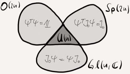
Prove that the intersection of any two of , , and is precisely as indicated by Figure 2.1.
The eigenvalues of a symplectic matrix occur either as pairs or or as complex quadruples
In particular, both and occur with even multiplicity.
2.1.1 Topology of
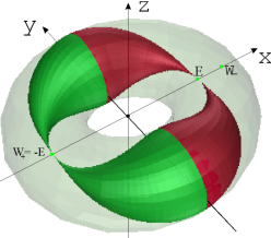
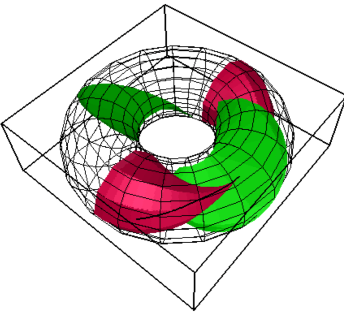
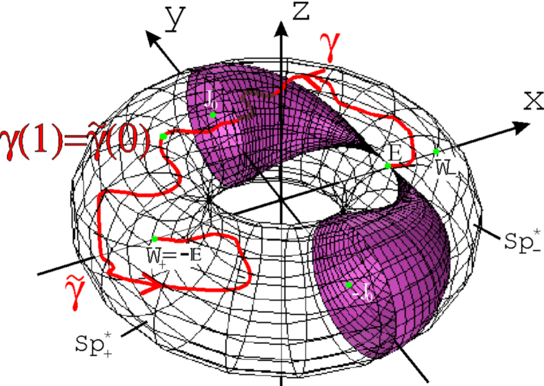
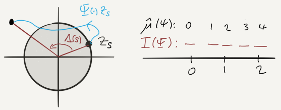
Major topological properties of , such as the fundamental group being or the existence of certain cycles, can nicely be visualized using the Gel′fand-Lidskiĭ \citesymptopGelfand:1958a homeomorphism between and the open solid 2-torus in . It is a diffeomorphism away from the center circle ; for details see also \citesymptop[App. D]weber:1999a. Consider the sets of all symplectic matrices which have in their spectrum.
| The set is called the Maslov cycle of . |
It consists of disjoint subsets which are submanifolds, called strata. For there are only two strata one of which contains only one element, namely the identity matrix ; see Figure 2.2 which shows in the Gel′fand-Lidskiĭ parametrization of , namely, as the open solid -torus in .
For the spectrum of the elements of there are three possibilities:
-
(pos. hyp.)
real positive pairs ; those with are ;
-
(neg. hyp.)
real negative pairs ; those with are ;
-
(elliptic)
complex pairs ; those enclosed by .
Exercise 2.1.4 (Eigenvalues of first and second kind).
Note that the set enclosed by has two connected components. What distinguishes them?333 Those whose eigenvalue of the first kind lies in the upper half plane, e.g. , lie in the same component, those where this location is the lower half plane lie in the other component. Suppose are eigenvalues of . Thus and the eigenvectors are linearly independent. Show that . If the imaginary part of this quantity is positive, then is called of the first kind, otherwise of the second kind. Show that one of is of the first kind and the other one of the second kind.
For , , where the eigenvalues can be quadruples the notion of eigenvalues of the first and second kind becomes important concerning stability properties of Hamiltonian trajectories: Two pairs of eigenvalues on can meet and leave , if and only if, eigenvalues of different kind meet.
2.1.2 Maslov index
Loops are continuous throughout Section 2.1.2. The map
| (2.1.2) |
is a strong deformation retraction of onto ; cf. Figure 2.1. So the quotient space is contractible. It is well known that the determinant map induces an isomorphism of fundamental groups. Consequently the fundamental group of is given by the integers. Define a map by
| (2.1.3) |
Maslov index – degree
An explicit isomorphism is realized by the Maslov index which assigns to every loop of symplectic matrices the integer
Exercise 2.1.5.
Show that the Maslov index satisfies the following axioms:
-
(homotopy)
Two loops in are homotopic iff they have the same Maslov index.
-
(product)
For any two loops we have
Consequently , hence where .
-
(direct sum)
If , then .
-
(normalization)
The loop , , has Maslov index .
Show that these axioms determine uniquely. [Hints: The problem reduces to loops in by (2.1.2). On diagonal matrizes and products of matrizes behaves nicely. A complex matrix is triangularizable via conjugation by a unitary matrix, continuously in . Diagonal elements are loops .]
Maslov index – intersection number with Maslov cycle
Looking at the Maslov cycle in Figure 2.4, alternatively at the Robbin-Salamon cycle ,444 Write in the form of a block matrix with four matrices and consider the function , . By definition the Robbin-Salamon cycle is the pre-image , i.e. consists of all with =0. Actually is partitioned by the submanifolds of codimension which consist of those with and is the complement of the codimension zero stratum . suggests that the Maslov index should be half the intersection number with either cycle of generic, that is transverse, loops .555 This is indeed the case: The Robbin-Salamon index of a generic loop is the intersection number with ; see definition in \citesymptop[§4]Robbin:1993a. The equality follows either by the formula in \citesymptop[Rmk. 5.3]Robbin:1993a or by the fact that satisfies, by \citesymptop[Thm. 4.1]Robbin:1993a, the first three axioms for in Exercise 2.1.5. To confirm (normalization) calculate . Hint: , intersection form above \citesymptop[Thm. 4.1]Robbin:1993a.]
2.1.3 Conley-Zehnder index of symplectic path
Paths and loops are continuous throughout Section 2.1.3. Consider the map
| (2.1.4) |
and note that the pre-image of is precisely the Maslov cycle . Let , , and be the subsets of on which this map is, respectively, different from zero, positive, and negative. Thus we obtain the partitions
Geometrically the Conley-Zehnder index of admissible paths , namely
can be defined as intersection number with the Maslov cycle of generic paths in starting at the identity and ending away from the Maslov cycle. Here generic not only means transverse to the codimension one stratum, but also in the sense that the paths depart from immediately into . The need for the latter condition can be read off from Figure 2.4 easily.
Exercise 2.1.6.
Following the original definition by Conley and Zehnder \citesymptop[§1]conley:1984a, pick a path . Then its endpoint lies in one of the two connected open sets or . Show that these sets contain, respectively, the matrices
Extend from its endpoint to the corresponding matrix inside the component of the endpoint. Consider the extended path . Define
and show that and that
Clearly taking the square of yields in either case. Hence the path closes up at time and therefore taking the degree makes sense.
The Conley-Zehnder index satisfies certain axioms, similar to those of the Maslov index in Exercise 2.1.5.
Theorem 2.1.7 (Conley-Zehnder index).
For the following holds.
-
(homotopy*)
The Conley-Zehnder index is constant on the components of .
-
(loop*)
for any loop .
-
(signature*)
If is a symmetric matrix of norm , then
where is the signature of and is the number of positive/negative eigenvalues of .
-
(direct sum)
If , then .
-
(naturality)
for any path .
-
(determinant)
.
-
(inverse)
.
The (signature) axiom normalizes . The -axioms determine uniquely; see e.g. \citerefFH[§2.4]salamon:1999a.
Remark 2.1.8 (Canonical Maslov and Conley-Zehnder indices).
Clockwise rotation appears naturally in Hamiltonian dynamics, cf. (1.0.10), since is compatible with , not . Thus it is natural and convenient to introduce versions of the Maslov and Conley-Zehnder indices normalized clockwise and denoted by and , respectively, namely
-
(2.1.5)
These indices are just the negatives of the standard anti-clockwise normalized indices, that is and . They satisfy corresponding versions of the previously stated axioms, e.g. (loop) becomes and is displayed in (1.0.15).
In the present text we use for Floer, and also Rabinowitz-Floer, homology the canonical (clockwise) version of the Conley-Zehnder index, because on cotangent bundles (see Section 3.5) these theories relate canonically to the classical action functional which requires no choices at all to establish Morse homology; see Remark 1.0.8.
The reason why we introduced here in great detail the standard (counter-clockwise) version is better comparability with the literature. It spares the reader continuously translating between the normalizations. So while we explain , the reader can conveniently consult the literature for details of proofs, and once everything is established for we simply note that .
Symmetric matrizes are rather intimately tied to symplectic geometry:
Exercise 2.1.9.
Show that for symmetric the matrizes and are elements of whenever .
Exercise 2.1.10 (Symmetric matrizes).
More generally, given a path of symmetric matrizes, show that the path of matrizes determined by the initial value problem
| (2.1.6) |
takes values in . Note that iff . Vice versa, given a symplectic path , then the family of matrizes defined by
| (2.1.7) |
is symmetric.
Exercise 2.1.11.
a) The map (2.1.4) provides a natural co-orientation666
A co-orientation is an orientation of the normal
bundle (to the top-diml. stratum).
of the Maslov cycle .
Does this co-orientation serve to define the Maslov index
as intersection number with ?
(For simplicity suppose .)
[Hint: Given this co-orientation, calculate for any generic loop
winding around ‘the hole’ once.]
b) Is the situation better for the Robbin-Salamon cycle
? Suppose and co-orient
by the increasing direction of the function in an earlier footnote.
Show that the intersection number with of the loop
is at and at .
c) For consider the parity of
defined in \citesymptop[Rmk. 4.5]Robbin:1993a. Check that for
the parity is at and at
. Check that the intersection number of loops
with co-oriented by -co-orientation times parity
recovers the Maslov index .
By now several alternative descriptions of the Conley-Zehnder index have been found, for instance, the interpretation as intersection number with the Maslov cycle of a symplectic path, even with arbitrary endpoints, has been defined by Robbin and Salamon \citesymptopRobbin:1993a; see Section 2.1.5. In case there is a description of in terms of winding numbers which we discuss right below.
For further details concerning Maslov, Conley-Zehnder, and other indices see e.g. \citesymptopArnold:1967a,conley:1984a,Robbin:1993a, Gutt:2014a-arXiv-link and\citerefFHsalamon:1999a.
Winding number descriptions of in the case
For the following geometric and analytic construction we recommend the presentations in \citesymptop[§8]Hofer:2003a and \citesymptop[§2]Hryniewicz:2015a. It is convenient to naturally identify with and with .
Geometric description (winding intervals \citesymptop[§3]Hofer:1999a). A path with uniquely determines via the identity
two continuous functions and . Note that and . Define the winding number of the point under the symplectic path , i.e. the change in argument of , see Figure 2.5,
by
The winding interval of the symplectic path is the union
of the winding numbers under of the elements of . The interval is compact, its boundary is disjoint from the integers iff , that is iff , and most importantly its length is less then . Thus, for , the winding interval either lies between two consecutive integers or contains precisely one of them in its interior. Thus one can define
for some integer . One verifies the -axioms in Theorem 2.1.7 to get that is the Conley-Zehnder index itself.
Observe that the winding number is an integer iff is a positive multiple of . But the latter means that is a positive eigenvalue of . Thus which shows that positive hyperbolic paths are of even Conley-Zehnder index. Similar considerations show that negative hyperbolic and elliptic paths both have odd Conley-Zehnder indices.
Analytic description (eigenvalue winding numbers, \citesymptop[§3]Hofer:1995b). The integer can be characterized in terms of the spectral properties of the unbounded self-adjoint differential operator on with dense domain , namely
where the family of symmetric matrices corresponds to via (2.1.7). Here we assume that the symplectic path is defined on and satisfies . This extra condition corresponds to periodicity .
The spectrum of the operator consists,
by compactness of the resolvent, of countably many
isolated real eigenvalues of finite multiplicity
accumulating precisely at .
Suppose that is eigenfunction
associated to an eigenvalue .
Note that cannot have any zero.
Thus we can write
and define its winding number by
.
This integer only depends on the eigenvalue ,
but not on the choice of eigenvector. So it is denoted by
and called the winding number of the
eigenvalue .
For each integer there are precisely two eigenvalues (counted
with mulitplicities) whose winding number is .
If there is only one such eigenvalue, its multiplicity is 2.
Moreover, if , then
.
Let be the largest negative eigenvalue
and the next larger one.
Define the maximal winding number among the negative eigenvalues
of the operator and its parity by
Theorem 2.1.12.
If , then .
2.1.4 Lagrangian subspaces
A symplectic vector space is a real vector space with a non-degenerate skew-symmetric bilinear form. So is necessarily even.
Exercise 2.1.13.
Show that, firstly, each symplectic vector space admits a symplectic basis, that is vectors such that
and, secondly, there is a linear symplectomorphism – a vector space isomorphism preserving the symplectic forms – to .
The symplectic complement of a vector subspace is defined by
In contrast to the orthogonal complement, the symplectic complement is not necessarily disjoint to , but and are still of complementary dimension (as non-degeneracy is imposed in both worlds) and . Thus the maximal dimension of is . Such , that is those with , are called Lagrangian subspaces. Equivalently these are characterized as the dimensional subspaces restricted to which vanishes identically.
A subspace is called isotropic if , in other words, if vanishes on , and coisotropic if .
Exercise 2.1.14 (Graphs of symmetric matrizes are Lagrangian).
Show that
is a Lagrangian subspace of if and only if is symmetric.
Exercise 2.1.15 (Natural structures on ).
Let be a real vector space and its dual space.777 Here is the dual space of the real vector space . Show that on a symplectic form is naturally given by . Show that both summands of are Lagrangian. Now pick, in addition, an inner product on , that is a non-degenerate symmetric bilinear form on . This provides a natural isomorphism , , again denoted by , which naturally leads to the inner product on . Moreover, on one obtains an inner product and an almost complex structure ; cf. (2.4.28). Show their compatibility in the sense that .
Exercise 2.1.16.
Show that the graph of a linear symplectomorphism is a Lagrangian subspace of the cartesian product equipped with the symplectic form that sends to . Note that the diagonal subspace is Lagrangian.
2.1.5 Robbin-Salamon index – degenerate endpoints
A symplectic path gives rise to the family of symmetric matrizes given by (2.1.7) for which, in turn, it is a solution to the ODE (2.1.6). A number is called a crossing if or, equivalently, if is eigenvalue of . In other words, if hits the Maslov cycle : The eigenspace must be non-trivial.
At a crossing the quadradic form given by
is called the crossing form. A crossing is called regular if the crossing form is non-degenerate. Regular crossings are isolated. If all crossings are regular the Robbin-Salamon index was introduced in \citesymptopRobbin:1993a, although here we repeat the presentation given in \citerefFH[§ 2.4]salamon:1999a, as the sum over all crossings of the signatures of the crossing forms where crossings at the boundary points are counted with the factor only. For the particular paths the Robbin-Salamon index
reproduces the Conley-Zehnder index.
Exercise 2.1.17.
a) Check the identity in the definition of . b) The factor at the endpoints is introduced in order to make invariant under homotopies with fixed endpoints. To see what happens homotop the path in Figure 2.4 to and calculate the crossing forms at in both cases.
In \citesymptopRobbin:1993a an index for a rather more general class of paths is constructed: A relative index for pairs of paths of Lagrangian subspaces of a symplectic vector space ; cf. Exercise 2.1.14. Here crossings are non-trivial intersections . The Conley-Zehnder index on is recovered by choosing the symplectic vector space and the Lagrangian path given by the graphs of relative to the constant path given by the diagonal . Indeed by \citesymptop[Rmk. 5.4]Robbin:1993a. Note that .
2.2 Symplectic vector bundles
Suppose is a vector bundle of real rank over a manifold-with-boundary of dimension ; where is not excluded. A symplectic vector bundle is a pair where is a family of symplectic bilinear forms , one on each fiber . Similarly a complex vector bundle is a pair where is a family of complex structures on the fibers , that is . Existence of a deformation retraction, such as in (2.1.2), of onto has the consequence that any symplectic vector bundle is fiberwise homotopic, thus isomorphic as a vector bundle,888 A vector bundle isomorphism is a diffeomorphism between the total spaces whose fiber restrictions are vector space isomorphisms. to a complex vector bundle called the underlying complex vector bundle.999 The complex structure , but not its isomorphism class, depends on . A Hermitian vector bundle is a symplectic and complex vector bundle such that is -compatible, that is is a Riemannian bundle metric on .
Proposition 2.2.1.
Two symplectic vector bundles and are isomorphic if and only if their underlying complex bundles are isomorphic.
Two proofs are given in [MS98, §2.6], one based on the deformation retraction (2.1.2), the other on constructing a homotopy equivalence between , the space of -compatible complex structures on a symplectic vector space, and the convex, thus contractible, non-empty space of all inner products on .
A trivialization of a bundle is an isomorphism to the trivial bundle which preserves the structure under consideration. A unitary trivialization of a Hermitian vector bundle is a smooth map
| (2.2.8) |
which maps fibers linearly isomorphic to fibers, that is is a vector bundle isomorphism to the trivial bundle, and simultaneously identifies the compatible triple on with the standard compatible triple on .
Proposition 2.2.2.
A Hermitian vector bundle over a compact Riemann surface with non-empty boundary admits a unitary trivialization.
The idea is to prove in a first step that for any path the pull-back bundle can be unitarily trivialized even if one fixes in advance unitary isomorphisms and over the two endpoints of . To see this construct unitary frames over small subintervalls of starting with a unitary basis of at some , extend to a small intervall via parallel transport, say with respect to some Riemannian connection on , and then exposed to the Gram-Schmidt process over . The coupling of the resulting unitary trivializations over the subintervals is based on the fact that the Lie group is connected. In the second step one uses a parametrized version of step one to deal with the case that is diffeomorphic to the unit disk . 101010 Trivialize along rays starting at the origin: Extend a chosen frame sitting at the origin simultaneously along all rays, say by parallel transport, along an interval . Now apply Gram-Schmidt to the family of frames and repeat the process on , and so on. Step three is to prove the general case by an induction that starts at step two and whose induction step is again by a parametrized version of step one, this time for the disk with two open disks removed from its interior (called a pair of pants).
2.2.1 Compatible almost complex structures
Given a symplectic manifold , consider an endomorphism of with . Such is called an almost complex structure on .111111 Such is called a complex structure or an integrable complex structure on , if it arises from an atlas of consisting of complex differentiable coordinate charts to . If, in addition, the expression
defines a Riemannian metric on , then is called an -compatible almost complex structure on . The space of all such is non-empty and contractible by [MS98, Prop. 2.63].
Exercise 2.2.3.
Pick and let be the Levi-Civita connection associated to . Suppose is a smooth vector field on , show (i) and (ii):121212 Part (iii) is less trivial; see [MS04, Le. C.7.1].
-
(i)
preserves and ;
-
(ii)
and are anti-symmetric with respect to ;
-
(iii)
.
2.2.2 First Chern class
Up to isomorphism, symplectic131313 equivalently, complex vector bundles, by Proposition 2.2.1 vector bundles over manifolds are classified by a family of integral cohomology classes of called Chern classes. If is a closed orientable Riemannian surface, the first Chern class is uniquely determined by the first Chern number which is the integer obtained by evaluating the first Chern class on the fundamental cycle . Thus, slightly abusing notation, in case we shall denote the first Chern number by . We cite again from [MS98].
Theorem 2.2.4.
There exists a unique functor , called the first Chern number, which assigns an integer to every symplectic vector bundle over a closed oriented Riemann surface and satisfies the following axioms.
-
(naturality)
Two symplectic vector bundles and over are isomorphic iff they have the same rank and the same Chern number.
-
(functoriality)
For any smooth map of oriented Riemann surfaces and any symplectic vector bundle it holds .
-
(additivity)
For any two symplectic vector bundles and
-
(normalization)
The Chern number of is where is the genus.
The proof is constructive, based on the Maslov index for symplectic loops: Pick a splitting such that as oriented manifolds. So the union of, say , embedded 1-spheres is oriented as the boundary of , say by the outward-normal-first convention. Given a symplectic vector bundle over , pick unitary141414 a symplectic trivialization (just required to identify with ) is already fine trivializations
| (2.2.9) |
and consider the overlap map defined by .
Exercise 2.2.5 (First Chern number).
Prove uniqueness in Theorem 2.2.4. Show that the first Chern number of is the degree of the composition
by verifying for the four axioms for the first
Chern number.
(The second identity for the Maslov index is obvious:
Just pick an orientation preserving parametrization
for each connected component of .)
[Hint: Show, or even just assume, first that
is independent of the choice of,
firstly, trivialization and, secondly, splitting.
Use these two facts, whose proofs rely heavily on
Lemma 2.2.6 below, to verify the four axioms.]
Lemma 2.2.6.
Let be a compact oriented Riemann surface with non-empty boundary. A smooth map extends to iff .
Exercise 2.2.7 (Obstruction to triviality).
Use the axioms to show that the first Chern number vanishes iff the symplectic vector bundle is trivial, that is isomorphic to the trivial Hermitian bundle .
Exercise 2.2.8 (First Chern class).
Suppose is a symplectic vector bundle over any manifold . Observe that the first Chern number assigns an integer to every smooth map defined on a given closed oriented Riemannian surface. Use the axioms to show that this integer depends only on the homology class of and so the first Chern number generalizes to an integral cohomology class called the first Chern class of .
The first Chern class of a symplectic manifold, denoted by or just by , is the first Chern class of the tangent bundle .
Exercise 2.2.9 (Splitting Lemma151515 There is a far more general theory behind called splitting principle; see e.g. [BT82, §21]. ).
Every symplectic vector bundle over a closed oriented Riemannian
surface decomposes as a direct sum of rank-2
symplectic vector bundles.
[Hint: View as complex vector bundle with -dual ,
so ;
cf. [GH78, p.414]. Remember (naturality).]
Exercise 2.2.10 (Lagrangian subbundle).
Suppose is a symplectic vector bundle over a
closed oriented Riemannian surface. If admits a Lagrangian
subbundle , then the first Chern number vanishes.
(Consequently the vector bundle is unitarily trivial by
Exercise 2.2.7.)
[Hint: The unitary trivializations (2.2.9)
identify Lagrangian subspaces.
Modify them so that each Lagrangian in
gets identified with the horizontal Lagrangian .
Then the overlap map will be of the form (2.1.3)
with , so the determinant is real
and the degree therefore zero.]
2.3 Hamiltonian trajectories
In the following we shall distinguish the analytic point of view (maps) from the topological, often geometrical, point of view (subsets, often submanifolds). We use the following terminology to indicate
Sometimes it is convenient to use one and the same term in both worlds and employ two adjectives to indicate the analysis or the geometry point of view: Since periodicity is a property of maps, whereas closedness (compact and no boundary) is a property of submanifolds, our convention is that
Closed geodesics are immersed circles and so are non-point closed orbits.
2.3.1 Paths, periods, and loops
Suppose is a manifold.
Definition 2.3.1 (Paths and curves, closed, simple, constant).
A path is a smooth map of the form
, whereas a finite path
is a smooth map that is defined on a compact
interval where .
The images and
are connected subsets of ,
called curves in .
In case we call , ,
alternatively , , a
point path and its image curve
a point.
Note: Point paths are automatically embeddings and points
embedded submanifolds.
A path , finite or not, is called simple if it is injective along the interior of the domain or, equivalently, if it does not admit self-intersections at times in the interior of the domain. The image of a simple path is called a simple curve. At the other extreme are paths, finite or not, whose images consist of a single point only. These are called constant paths. Note: A constant path is simple iff it is a point path.
We say that a finite path closes up with order if initial and end point coincide, together with all derivatives up to order . In case all derivatives close up () we speak of a finite path that closes up smoothly, if in addition we speak of a loop of period . (For we already assigned the name point path. A loop can be constant though.)
There are corresponding notions in other categories, e.g. the elements of are called paths, there are e.g. loops and so on.
Definition 2.3.2 (Paths, periodic and non-periodic).
Consider a path . If there is a real such that , then is called a periodic path and a period of . One also says that the path is -periodic. If there is no such , then is called non-periodic. By definition is considered a period of any path, called the trivial period. Let be the set of all periods of , including the trivial period .
Observe that iff is a non-periodic path and iff is a constant path. Do not confuse finite path that closes up with periodic path – the domains and are different. However, a finite path closing up with all derivatives comes with an associated -periodic path
Note that if is a point path, then is a constant path. Vice versa, a non-constant -periodic path is the infinite concatenation of the closed finite paths , .
Exercise 2.3.3.
Given a path , show that is a closed subgroup of . With the convention define the minimal or prime period
Show that the period group of a path comes in three flavors, namely
| (2.3.10) |
[Hint: Consult [PP09, Prop. 1.3.1] if you get stuck.] If the period groups of two paths that have the same image curve are equal, will they in general become equal after suitable time shift?
Definition 2.3.4 (Prime and divisor parts, loops).
A divisor part of a periodic path is a finite path of the form
| (2.3.11) |
one for each period . For the map on the quotient161616 By we also denote “freezing the variable ”, but application context should be different.
| (2.3.12) |
is the loop associated to the non-zero period of the non-constant path . To the trivial period we associate the point path
which we do not call a loop. A loop is a map of the form (2.3.12). In case the minimal period is positive and finite we denote the associated divisor part and loop by
| (2.3.13) |
called the prime part and the prime loop of a (non-constant) periodic path. It is useful to call the loop also the prime loop of any of the loops associated to a positive period of . A simple loop is an injective prime loop , equivalently, the finite path must be simple. Observe that is a -fold cover of .
Exercise 2.3.5.
Find a path whose prime part is not simple. Show that a simple loop which is an immersion is an embedding (an injective immersion that is a homeomorphism onto its image) of the unit circle.
Do not confuse the prime period of a path with the time of first return, often called time of first continuous return or of order zero and denoted by , namely but at earlier times .171717 Similarly define the time of first return of order by the condition , together with all derivatives up to order , and this is not the case at any earlier time . To see the difference consider a figure eight with being the crossing point. For trajectories of smooth autonomous vector fields both notions coincide, prime parts are automatically simple, and prime loops are circle embeddings; cf. Exercise 2.3.19! For a periodic immersion , thus non-constant, an associated loop is simple iff it is an embedding iff it is the prime loop.
Remark 2.3.6 (Negative periods).
Definition 2.3.7 (Concatenation of finite paths and loops).
(i) Consider two consecutive finite paths, that is and such that ends at the point at which begins, together with all derivatives.181818 If the domains are and replace by . The concatenation of two consecutive finite paths is the finite path defined by following first and then , notation
Finite paths closing up with all derivatives are self-concatenable: For consider the -fold concatenation ; it is traversed backwards in case , see (2.3.11). In case denote by
| (2.3.14) |
the associated -periodic loop; mind convention (2.3.12) if . To associate the point path with domain .
Definition 2.3.8 (Time shift and uniform change of speed).
Certainly if a path is -periodic, then so is any time shifted path
The operation uniform change of speed applied to a loop , namely
| (2.3.15) |
produces the new prime period , if , and .
Remark 2.3.9 (In/compatibilities).
The operation of -fold self-concatenation of a -periodic loop is compatible with ODEs and also preserves periods in the sense that is still a period after the operation. Period preservation also holds true for uniform integer speed changes , but for these do in general not map ODE solutions to solutions. Examples are integral trajectories of a vector field ( order ODE). However, there are important cases where solutions are mapped to solutions, e.g. periodic geodesics ( order ODE).
Exercise 2.3.10 (Loops and periods – immersed case).
An immersion is a smooth map whose differential is injective at every point. Starting from Definition 2.3.1 redo all definitions and constructions replacing path by immersed path and investigate if and how things change.
Exercise 2.3.11 (Loops and periods – embedded case).
Consider only immersed paths . Then a loop is an embedding iff it is simple, in which case it is prime (but prime is not sufficient). Investigate if and how the previous constructions change on the space of embedded loops. A crucial observation is that, given a non-constant periodic trajectory of an autonomous smooth vector field on , an associated loop is embedded iff it is prime.
2.3.2 Hamiltonian flows
Throughout is a symplectic manifold and, as usual, everything is smooth.
Autonomous Hamiltonians
Given a function , by non-degeneracy of the identity of -forms
| (2.3.16) |
determines a vector field on , called the Hamiltonian vector field associated to or the symplectic gradient of . The function is called the Hamiltonian of the dynamical system and it is called autonomous since it does not depend on time. For -compatible almost complex structures the Hamiltonian vector field is given by
| (2.3.17) |
where the gradient is taken with respect to the induced Riemannian metric, that is is determined by . We denote the flow generated by the Hamiltonian vector field of an autonomous Hamiltonian by , alternatively by , as opposed to the greek letter used in case of non-autonomous Hamiltonians which are usually denoted by .
An energy level is a pre-image set where is an autonomous Hamiltonian. It is called an energy surface if is a regular value of , notation . Hence energy surfaces contain no singularities (zeroes) of , equivalently, no stationary points191919 This means that for all times or, in other words, for the members of the whole family . For distinction we use the term fixed point in the context of an individual map: If , then is called a fixed point (of the map ). of the flow, and by the regular value theorem is a smooth codimension one submanifold of . Most importantly, the Hamiltonian flow preserves its energy levels:
| (2.3.18) |
for every initial condition .
Exercise 2.3.12.
Remark 2.3.13 (Periodic vs closed and autonomous vs time-dependent).
a) Suppose the flow of is complete, that is . The solution , , of with is called a Hamiltonian path or a flow trajectory – note the domain . A solution is either a line immersion (embedded or with self-tangencies , but not self-transverse) or it is constant . The image of a flow trajectory is called a flow line or an integral curve of the Hamiltonian vector field. If the solution path forms a loop (possibly constant but by definition of loop) we call it a Hamiltonian loop or a periodic orbit of period (note the circle domain) and its image a closed orbit.
b) Autonomous (time-independent) vector fields on a manifold : Their closed orbits are closed submanifolds of dimension, either one (an embedded circle), or zero (a point). For a non-constant periodic trajectory of the prime period coincides with the time of first continuous return.
c) Non-autonomous vector fields on : Here any geometric property of the image of a non-constant trajectory is lost, in general.202020 Unless one looks at the corresponding trajectory in . This is due to the possibility that could be zero for a time interval of positive length during which the trajectory will rest at a point, say . Switching on again a suitable vector field one can leave in any desired direction. Compared to the autonomous case , not only the immersion property is lost, but there can be arbitrary self-intersections. So is in general nothing but a subset of . The same argument shows that the notion of time of first return, even with infinite order, is meaningless, it would not imply periodicity of a non-constant trajectory . For these reasons, in case of a non-autonomous vector field, we do not call the image of a periodic trajectory a closed orbit, it will be called just an image. However, periodic solutions may exist and these will still be called periodic orbits.
d) Concerning solutions of autonomous order ODE’s see Exercise 2.3.19.
Remark 2.3.14.
Given , note that is a -periodic trajectory of iff is a -periodic trajectory of . More generally, that is a -periodic trajectory of a -periodic vector field is equivalent to being a -periodic trajectory of the -periodic vector field .
Remark 2.3.15 (Multiple cover problem – variable period).
This doesn’t refer to change of speed, but to path concatenation: Given a -periodic trajectory of , consider that same map instead of on on the larger domain , , to get a periodic trajectory times covering – same speed but -fold time.
Proposition 2.3.16 ( and small Hamiltonians, [HZ11, §6.1]).
Suppose is a closed symplectic manifold. Sufficiently small Hamiltonians do not admit non-contractible -periodic orbits. Sufficiently small autonomous Hamiltonians do not admit -periodic orbits at all – except the constant ones sitting at the critical points.
Idea of proof.
Pick an -compatible almost complex structure to conclude that the length of a periodic orbit of period one is small if the Hamiltonian is small, autonomous or not. Indeed
But a short loop in a compact manifold is contractible and its image is covered by a Darboux chart. For autonomous the argument on page 185 in [HZ11] shows that whenever the Hessian of is sufficiently small. ∎
Non-autonomous Hamiltonians
A time dependent Hamiltonian , notation , generates a time dependent Hamiltonian vector field by considering (2.3.16) for each time . One obtains a family of symplectomorphisms212121 A symplectomorphism is a diffeomorphism preserving the symplectic form: . on , called the Hamiltonian flow generated by , via
| (2.3.19) |
The family222222 If depends on time, it is wise to keep track of the initial time . As indicated in (2.3.19) we shall always use . The notation helps to remember that is in general not a composition of and . To obtain the composition law one would have to allow for variable initial times, not just . For simplicity . is called a complete flow if it exists for all . Important examples are autonomous Hamiltonians and periodic in time Hamiltonians , both on closed manifolds. A Hamiltonian trajectory, is a path of the form with . In case is a loop we call it a Hamiltonian loop. In either case satisfies the Hamiltonian equation
Hamiltonian flows, autonomous or not, preserve the symplectic form. By definition232323 Alternatively, defining axiomatically, our definition becomes Thm. 2.2.24 in [AM78]. of the Lie derivative and Cartan’s formula one gets
| (2.3.20) |
This shows that the family of diffeomorphisms generated by the family of vector fields preserves , that is , if and only if the -form is closed.242424 Such vector fields are called symplectic, generalizing the Hamiltonian ones. This holds, for instance, if is Hamiltonian ().
Periodic orbits and their loop types
Remark 2.3.17 (Loops, periodic orbits, closed characteristics).
Topology (Subsets). A loop is a simple, thus prime, loop if it admits no self-intersections, in symbols . Given two non-constant loops and , if for some integer , one says that is -fold covered by , or a multiply covered loop in case , in symbols . Two loops and are called geometrically distinct if their image sets are not equal. Otherwise, they are geometrically equivalent, in symbols
Geometrically equivalent loops, although having the same image set, certainly can be very different as maps. For instance, subloops of a figure-eight can be traversed a different number of times or in a different order.252525 While we require loops to be smooth, they do not need to be immersions. To go smoothly around a corner, just slow down to speed zero and accelerate again afterwards.
Analysis (Maps). Whereas any loop in a manifold is a periodic orbit of some periodic vector field , only the rather restricted class of embedded loops arises as (prime) periodic orbits of autonomous vector fields; see Exercise 2.3.18. By (2.3.10) the prime loop of a non-constant periodic trajectory of an autonomous vector field is a circle embedding. Moreover, still in the autonomous case, two periodic orbits are geometrically distinct iff their images are disjoint and, in the non-constant case, geometrically equivalent iff one -fold covers the other one.
Geometry (Submanifolds). Suppose is an autonomous vector field on a manifold . Let be the set of loop trajectories , in other words, periodic orbits, all periods , constant solutions not excluded. Let be the subset of the non-constant ones. The sets of equivalence classes
| (2.3.21) |
correspond to the set of closed orbits of , respectively the non-point ones. The latter are disjoint embedded circles tangent to , disjoint to each other. Representatives and of the same element of are multiple covers of a common simple periodic orbit . In other words, the elements of the set are in bijection with those embedded circles whose tangent bundle is spanned by the vector field along . Technically one says that such are integral submanifolds of the (in general, singular) distribution of lines (and possibly points) along . We call these the integral circles of the vector field . The set corresponds to the integral circles of , whereas includes, in addition, the 0-dimensional integral submanifolds, namely, the zeroes, also called singularities, of the vector field .
In Chapters 4 and 5 we will deal with the following special case: The manifold is a closed regular level set of an autonomous Hamiltonian on a symplectic manifold and is the Hamiltonian vector field. Note that in this case there are no zeroes of , hence no constant solutions, on by regularity of the value . In fact, the vector field spans what is called the characteristic line bundle and this is true for whenever is a regular level set of a Hamiltonian ; see (4.1.3). Thus
| (2.3.22) |
denotes the set of integral circles of the characteristic distribution of real lines along . In this context the elements of are called the closed characteristics of the regular level set .
Exercise 2.3.18 (Loops are generated by vector fields).
a) A loop in is the trajectory of some periodic vector field
.
b) An embedded loop in is a trajectory
of some autonomous vector field .
[Hints: First case , graph of in , cutoff functions.]
Exercise 2.3.19 (Prime periodic geodesics are self-transverse, not self-tangent).
Let be a Riemannian manifold with Levi-Civita connection . Suppose the path satisfies the order ODE . The equation implies that the speed of a solution is constant in time . Hence all non-constant solutions are immersions, called geodesics. If a geodesic admits a positive period it is called a periodic geodesic often denoted by or to indicate the period in question. Its image is an immersed circle, called a closed geodesic. There are precisely two options. Such is
-
-
either self-transverse, then is the prime loop of , called a prime periodic geodesic, or
-
-
a -fold cover, where , of an underlying prime periodic geodesic.
Self-transverse means that whenever two arcs of meet in they intersect transversely. In this case there is just a finite number of intersection points by compactness of the domain.
a) Show that the two options are characterized by the two possibilities whether the set of times such that has more than one pre-image262626 In symbols . Such is called a multiple or a double () point. under is a finite set or an infinite set (thus equal to the circle domain itself).
b) Why are there no non-self-tangent self-intersections of trajectories of autonomous vector fields, but for geodesics they can appear?
2.3.3 Conley-Zehnder index of periodic orbits
Given a symplectic manifold , consider a -periodic family of Hamiltonians with Hamiltonian flow . Let be the set of -periodic orbits.
Exercise 2.3.20.
Check that , , provides a bijection between the set of -periodic orbits and the set of fixed points of the time-1-map corresponding to initial time zero. [Hint: Recall that abbreviates .]
A -periodic orbit is called non-degenerate if is not an eigenvalue of the linearized time--map, that is
| (2.3.23) |
Exercise 2.3.21.
Exercise 2.3.22 (Finite set).
If the manifold is closed and all -periodic orbits are non-degenerate, then the set , hence , is a finite set.
In addition to non-degeneracy, suppose the loop trajectory is contractible. Fix an extension of , namely a smooth map that coincides with on . Moreover, pick an auxiliary -compatible almost complex structure , so the Hermitian vector bundle with admits a unitary trivialization by Proposition 2.2.2, that is identifies the compatible triples and where rotates counter-clockwise and corresponds to . Restriction to the boundary provides a unitary trivialization, say , of the pull-back bundle . These choices provide a symplectic path defined by
| (2.3.24) |
The standard and the canonical Conley-Zehnder indices of the non-degenerate -periodic orbit are defined and related by
| (2.3.25) |
In general these indices depend on the spanning disk , unless . Sometimes it is useful to denote by or even by .
Exercise 2.3.23.
Show that and that . Show that does not depend on the particular unitary trivialization . Show that is independent of the choice of if vanishes on .
Exercise 2.3.24 (Critical points are periodic orbits).
Suppose is a non-degenerate critical point of a time independent function . Then the constant -periodic orbit is non-degenerate and the canonical Conley-Zehnder index and the Morse index of , see Section 3.1.1, are related by
| (2.3.26) |
whenever and where . To obtain the first displayed formula, pick an -compatible almost complex structure , the induced metric , and an orthonormal basis of eigenvectors of the Hessian of at and denote the corresponding Hessian matrix by .272727 One has for , but for . Apply the axiom .
2.4 Cotangent bundles
Cotangent bundles are the phase spaces in the Hamiltonian formulation of classical mechanics. Given the tremendous success of the theory in physics, not to mention daily life, one wouldn’t risk much predicting that these bundles should have a distinct position in the mathematical world as well. Indeed
| Cotangent bundles over a manifold |
-
(S1)
admit a canonical symplectic form and a canonical -form given by282828 Local coordinates on induce the diffeomorphism taking to and identifying with .
The Liouville form is characterized by the property that
(2.4.27) for every -form , so one calls the tautological 1-form;
-
(S2)
admit a canonical Lagrangian subbundle of the tangent bundle, namely292929 The previous coordinates identify each symplectically with the Lagrangian .
-
(S3)
admit along the zero section a natural Lagrangian splitting303030 is a direct sum: Linearize the composition of injection and surjection to get . So since ranks add up.
The isomorphisms313131 It suffices to show either surjectivity or injectivity (equal dimension of domain/codomain). As is injective it is an isomorphism onto its image with inverse . Assuming with means . So , as is Lagrangian: The restriction is zero as is the zero section. and are determined in terms of the inclusion , , by
and where
-
(S4)
have trivial first Chern class in the sense that for every oriented closed323232 The argument involves Poincaré duality. Closedness: Push the obstruction to infinity. submanifold . If , then .333333 If use Exercise 2.2.10. In general, let be the -dual of the vector bundle . Then by [GH78, p.414] and as the restriction of to is a non-vanishing section; cf. \citesymptop[App. B.1.7]weber:1999a.
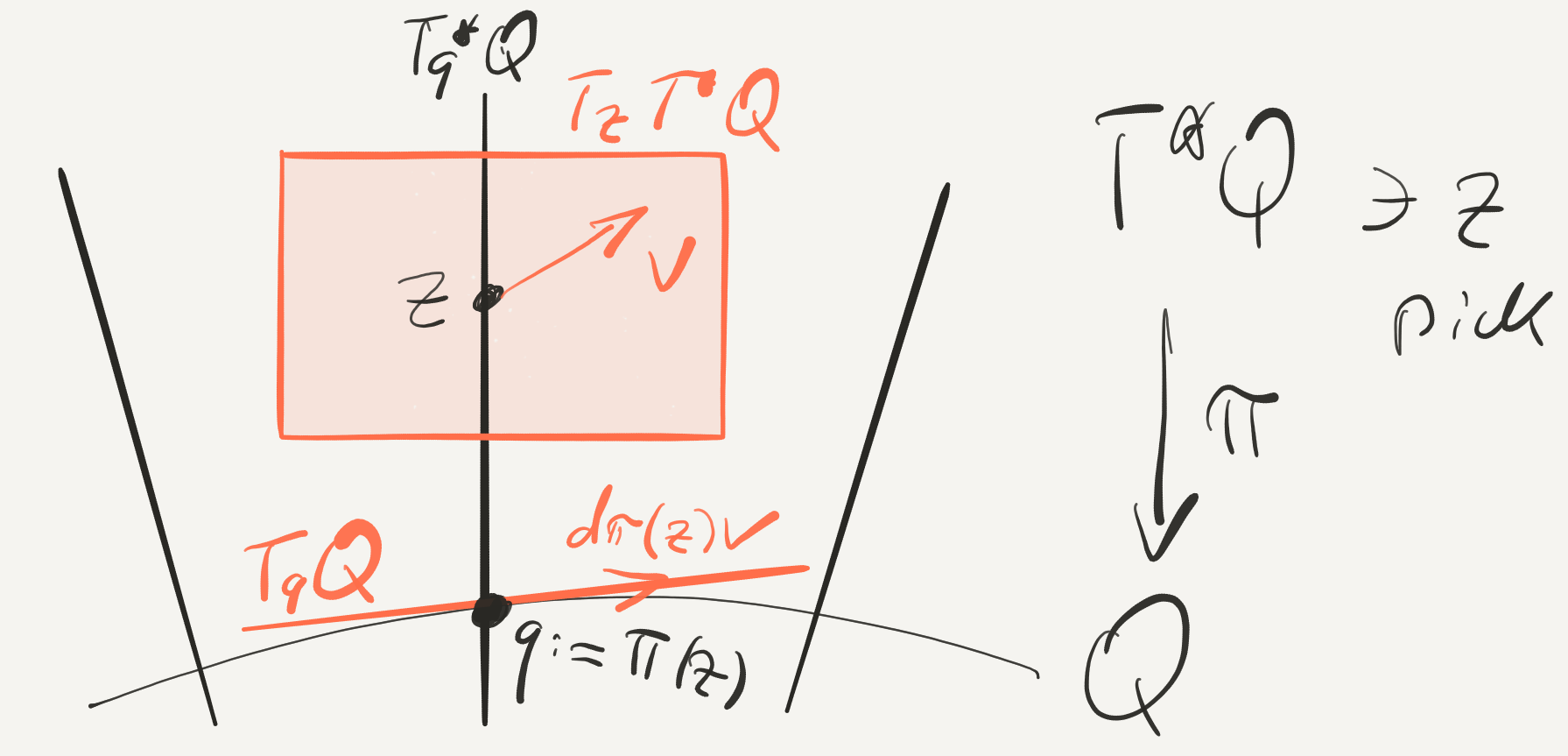
To get in all the other structures introduced in earlier sections is rather simple:
| Pick a Riemannian metric on to obtain |
-
(H1)
a global Lagrangian splitting defined pointwise by the isomorphism which takes the derivative of a curve in to the pair of derivatives, namely
The isomorphism takes to extending the one in (S3);
-
(H2)
a canonical Hermitian structure on defined pointwise for on by
(2.4.28) Concerning notation see Exercise 2.1.15. Throughout we denote by not only the Riemannian metric on , but also the induced isomorphism
Exercise 2.4.1.
Prove properties (S1–S4) and (H1–H2).343434 For details of the proof of (H1–H2) see e.g. \citesymptop[App. B.1.2–B.1.4]weber:1999a.
Exercise 2.4.2.
Any diffeomorphism of a manifold lifts to a symplectomorphism of the cotangent bundle
defined by . Prove that . What can one say if is a Riemannian manifold and is an isometry ()?
Exercise 2.4.3.
Suppose the vector field generates a -parameter group of diffeomorphisms . Consider the corresponding group of symplectomorphisms of and denote by the generating vector field, that is
Show that is the Hamiltonian vector
field of the function .
[Hint: Observe that
by the previous exercise and Cartan’s formula and
that .]
2.4.1 Electromagnetic flows – twisted cotangent bundles
Classical mechanics describes the motion of a particle of unit mass and unit charge located at time at position in a configuration space, a manifold . The electromagnetic system353535 Maxwell’s equations for a magnetic field and an electric field in are Here is the magnetic vector potential and the electric scalar potential. The Lorentz force law of a particle of mass and charge at position is (cf. \citesymptop[§1.1.2]arnold:2006a) is described by the following three structures on : A Riemannian metric (providing kinetic energy), a smooth one form (the magnetic potential), and a smooth function (the electric potential).
Exercise 2.4.4 (Reformulating Maxwell’s equations).
Let us reformulate (some of) Maxwell’s equations on in terms of quantities which are at home on manifolds – differential forms (see e.g. [BT82, War83]). Consider with its natural orientation and the euclidean metric . One-forms are in bijection with vector fields , just identify components:
Let us indicate the isomorphism by writing . Consider the isomorphism which relates the degree of the differential forms by and is determined on the elements of the natural bases by
and cyclic permutations. Note that .363636 More generally, on odd dimensional space , but on even dimensional space on forms of even/odd degree. With check373737 To corresponds .
| Remark | |||||
|---|---|---|---|---|---|
| magnetic potential | |||||
| exact magnetic field | |||||
| magnetic field, requires | |||||
| () | |||||
| velocity | |||||
| explicit calculation | |||||
| Lorentz force | |||||
This shows that the Lorentz force experienced by a particle of unit mass and unit charge is determined in terms of the closed 2-form encoding the magnetic field by the identity
| (2.4.29) |
Concerning differential forms in electrodynamics see e.g. \citesymptopDeschamps:1981a,Bott:1985a,Warnick:2014a.
Exercise 2.4.5 (Twisted symplectic structures ).
Suppose is a closed 2-form on the closed manifold .
Denote by the bundle
projection.
Show that is a symplectic form on .
Now fix a Riemannian metric on and check that the
identity
pointwise at and determines a fiber preserving anti-symmetric vector bundle map , i.e. fiberwise the map is linear and anti-symmetric. The map is the Lorentz force associated to the magnetic field ; see e.g. \citesymptopContreras:2004a. We chose the minus sign in order to match the classical scenario (2.4.29) in ; cf. \citesymptopBarros:2005a.
Exercise 2.4.6 (Twisted geodesic flow).
A curve solves the Euler-Lagrange equations (2.4.30) associated to the Lagrangian given by
where is called kinetic energy, if and only if (cf. \citesymptop[§2]Ginzburg:1996a) the pair is an integral curve of the Hamiltonian vector field associated to the Hamiltonian and the twisted symplectic structure on given by
The flow of is called twisted geodesic flow, its flow lines twisted geodesics. Note: In the Hamiltonian formulation there is no need that the magnetic field is exact, any closed 2-form on will do by Exercise 2.4.5.
Concerning existence of periodic electromagnetic trajectories we recommend the (older) survey \citesymptopGinzburg:1996a and the comments \citesymptopGinzburg:2001b. For more recent results see e.g. \citerefRFMerry:2011a and references therein.
Lagrangian and Hamiltonian formalism
The Lagrangian formulation of the dynamics is as follows. Given two points , the motion of the particle is a curve with extremizing the classical action functional
Here the electromagnetic Lagrangian of the system is given by
The extremals (critical points) are the solutions of the Euler-Lagrange equations which in local coordinates can be written as
| (2.4.30) |
For the physics behind we recommend \citesymptopFeynman:1964a. For the variational theory in the more general setting of Tonelli Lagrangians383838 A Lagrangian is Tonelli if it is fiberwise uniformly convex and superlinear. see e.g. \citesymptopmazzucchelli:2012a or \citerefRFAbbondandolo:2013c.
The Hamiltonian description of the system replaces the Lagrangian by its Legendre transform called the electromagnetic Hamiltonian of the system and given by
where we substituted according to . The dynamics of the particle on is then determined by the Hamiltonian vector field .
Alternatively, the dynamics of the same particle is described by the Hamiltonian vector field associated to the standard non-magnetic Hamiltonian
and a magnetically twisted symplectic structure. This alternative description works not only for exact magnetic fields , but for any closed 2-form on ; cf. \citesymptop[Thm. 2.1 (ii)]Ginzburg:1996a.
Exercise 2.4.7.
Hamiltonian dynamics of and coincides.
For further details of the relation of symplectic geometry and classical mechanics see e.g. [Arn78] or \citesymptop[Ch. 3]Arnold:2001b or \citesymptop[§1, §4]arnold:2006a.
alpha
Chapter 3 Fixed period – Floer homology
Towards Floer homology
Consider a symplectic manifold . Given an autonomous Hamiltonian , it is an interesting but rather challenging problem to investigate the set “of geometrically distinct closed orbits” of the Hamiltonian vector field on a given regular energy level . A little thought reveals that this cannot be a set of Hamiltonian loops , but rather it should be a set of equivalence classes of such or, in geometric terms, of their images – embedded circles tangent to the Hamiltonian vector field . These circles form the set of closed characteristics of on ; cf. (2.3.22).
Back to Hamiltonian loops (circle-parametrized closed orbits). Let us simplify the problem, firstly, by searching for loop trajectories of without taking any equivalence classes at all, and secondly, by just focussing on the plain existence problem. Let us break this further down into smaller pieces.
Period one. The problem reduces to detect Hamiltonian loops of period one: A -periodic trajectory of on the level set corresponds to the -periodic trajectory of on the level set (); indeed . So there is a little price to pay: One looses the freedom to fix an energy value . (The notion of energy value/level is lost anyway as soon as one allows time-dependent Hamiltonians.) So let us then investigate the set of -periodic loop trajectories of . Two loops and are geometrically distinct if their images are disjoint subsets of , otherwise they are equivalent ; cf. Remark 2.3.17.
There are two problems with autonomous Hamiltonians concerning non-constant Hamiltonian loops . Suppose you found such of period .
-
(multiple covers)
How can you find out a Hamiltonian loop does not multiply cover another one ? In other words, is the prime period of ?
-
(degeneracy)
A non-constant Hamiltonian loop provides an family via time-shift
The multiple cover problem makes it difficult to decide if a newly detected periodic orbit, say in the form of a critical point of a functional on loop space, is geometrically different from known ones. The fact that the elements of are never isolated obstructs reformulating the problem in terms of Morse theory, a powerful tool to analyze sets of critical points in terms of topology.
Non-autonomous -periodic Hamiltonians and their -periodic orbits. Both problems can be avoided by allowing time-dependent Hamiltonians and directing attention to the set of -periodic Hamiltonian loops with respect to ; see (2.3.19). Is there a lower bound for the cardinality uniformly in ? in fact, this problem reduces to study , the set of contractible 1-periodic Hamiltonian loops:
Contractible -periodic Hamiltonian loops and closedness of . For the special case of small autonomous Hamiltonians all -periodic orbits are constant by Proposition 2.3.16, so there are no non-contractible ones. But a small Hamiltonian is obtained by multiplying any given by a small constant . Really? Correct, at least, if is closed. So from now on we assume closedness of – conveniently guaranteeing completeness of flows – and aim for a lower bound for the cardinality of the set , uniformly in .
Assumption 3.0.1.
Arriving at Floer’s ideas. It was well known before Floer that the contractible -periodic Hamiltonian loops are precisely the critical points of a (possibly multi-valued) functional , but at the time it seemed that this functional was “certainly not suitable for an existence proof.” \citerefFH[(1.5)]Moser:1976a. However, this changed with the success of Rabinowitz \citerefCGRabinowitz:1978a in applying minimax methods to detect critical values of – and with Floer’ s rather different idea \citeintrofloer:1988a to overcome the obstruction presented by infinite Morse index and coindex, namely, by looking at a relative index between critical points – which is finite! Thereby Floer discovered relative Morse theory and successfully reformulated the problem. Floer’s insights also included departing from looking at the gradient equation as a formal ODE on the loop space, but instead noticing that it represents a well posed PDE Fredholm problem for maps from the cylinder into the manifold itself (whenever suitably compactified by imposing non-degenerate Hamiltonian loops to sit at ). Assuming transversality, the dimension of the associated moduli space is finite, as it is the Fredholm index which itself is given by the spectral flow, the relative Morse index, along a flow cylinder. Non-degeneracy amounts to being a Morse functional, this holds true for generic , and in good cases (say ) the relative index becomes the difference of an absolute index associated to the non-degenerate Hamiltonian loops – the Conley-Zehnder index of Section 2.1.3. The fundamental results of Floer’s construction are the lower bounds (1.0.1) and (1.0.2) proving the Arnol′d conjecture \citeintrofloer:1989a in many cases; in general see \citerefFHFukaya:1999a,Liu:1998a.
Back to autonomous Hamiltonians: Closed characteristics. Given an autonomous Hamiltonian , a natural approach to analyze the set of closed integral manifolds of , see (2.3.21), would certainly be – in view of Floer’s estimate – to focus on in a first step: Approximate in an appropriate topology by non-degenerate, in general time--periodic, Hamiltonians . By Floer’s estimate every set is non-empty, so picking one element for every provides a sequence of Hamiltonian loops. Now one can try to extract a convergent subsequence using the Arzelà-Ascoli Theorem 3.2.10 and show that the limit loop, say , satisfies the equation of the limit Hamiltonian. There are two problems.
I. Firstly, the Hamiltonian limit loop , in fact already some or all of the , could be constant. This is excluded if the energy hypersurface of is known to be regular, that is if is a regular value of . Action filtered Floer homology may help sometimes; see Section 3.4.5 and e.g. \citerefFHweber:2006a.
II. The second problem are multiplicities. If you get two, or more, limit
solutions this way and suppose you even already know that they
are different and non-constant elements of , say by having information
about the action values and .
Even then, how would one decide whether
and are geometrically distinct or whether
one multiply covers the other one?
It helps looking at the particular Hamiltonian loops on a cotangent
bundle over a closed Riemannian manifold which correspond to
geodesics in the base manifold and remembering
Bott’s analysis \citerefFHBott:1956a of how the Morse index changes
under iterations .
For Hamiltonian loops the corresponding
index formulae have been pioneered by Long \citerefFHLong:2002a.
For recent tremendous success of studying iterations,
in a slightly different direction though,
see Ginzburg’s proof\citerefFHGinzburg:2010b of the
Conley conjecture.
See \citerefFHGinzburg:2015b for a recent survey about
existence of infinitely many simple periodic orbits.
Cotangent bundles and loop spaces. If one gives up the compactness requirement and looks at the class of symplectic manifolds given by cotangent bundles over closed Riemannian manifolds , say spin (thus orientable), equipped with physical Hamiltonians of the form kinetic plus potential energy and a natural almost complex structure , then Floer homology is totally different: It does not represent singular homology of , but it is naturally isomorphic to singular homology of the free loop space ; cf. Section 3.5. If is not simply connected, then there is one isomorphisms for each component of , so here Floer homology even detects non-contractible periodic orbits.
Outline of Chapter 3
Consider a Hamiltonian . Motivated by the Morse complex Floer’s program, see \citeintrofloer:1989a, is to use the symplectic action functional
cf. (3.2.11), as a Morse function to construct a Morse type chain complex.
In Section 3.1 we briefly recall the usual construction of the Morse complex associated to a Morse function on a closed Riemannian manifold of dimension by using the critical points as generators, the Morse index as grading, and counting downward gradient flow lines to define a boundary operator. We also recall the geometric realization of the Morse cochain complex using the same generators and grading, but counting upward flow lines.
Section 3.2 is devoted to a detailed study of the action functional starting with a list of serious deficiency and explaining sign conventions. Then we calculate the differential and, with the help of a family of -compatible almost complex structures, also the gradient of . This shows that the critical points are precisely given by the set
of -periodic contractible Hamiltonian loops.
We calculate the Hessian operator
of at a critical point
to define non-degeneracy of critical points.
Next we insert an excursion to Baire’s category theorem
trying to separate the surrounding and easily confusable notions of
“residual” and “second category” subsets.
The purpose is to detail the informal notion of genericity
in theorems like the one asserting that is Morse for generic
(“transversality on loops”).
Given Section 3.2,
we define, for generic , the Floer chain group
as the vector space generated by the finite set of
contractible -periodic orbits and graded by the canonical
Conley-Zehnder index in (2.3.25):
Section 3.3 introduces the substitute for the non-existent downward gradient flow of on , namely, solutions to Floer’s elliptic PDE111 Gromov’s \citeintrogromov:1985a -holomorphic curve equation is , now add a lower order perturbation . Here we have a -holomorphic curve equation where . Alternatively, time reflection relates the solutions of the displayed equation to solutions of the perturbed -holomorphic curve equation .
called Floer cylinders or Floer trajectories. A Floer trajectory defines what we informally call a “flow line” or “integral curve” in the loop space, namely, the image set . Any two trajectories producing the same flow line differ by composition with time-shift . It is useful to switch view points using the correspondence “cylinder in ” “path in ”, namely
Back to Floer cylinders .
Imposing as asymptotic boundary conditions
at Hamiltonian loops
we call a connecting trajectory from to .
Let be the space of
all of them. At this point we insert Section 3.3.2
on relevant elements of Fredholm theory needed to analyze under which
conditions the spaces are manifolds and to calculate
their dimensions. Since is Morse all asymptotic boundary
conditions are non-degenerate. This causes
the operators defined by linearizing Floer’s
equation at any connecting trajectory
to be Fredholm. For the manifold property of
and the dimension formula
one needs to make sure that is onto, often referred to as
“transversality on cylinders”.
But this can be achieved for generic again.
The necessary perturbation not only preserves the Morse property, but
even the set of critical points.
The machinery to deal with transversality issues,
be it non-degeneracy of the critical points of
or surjectivity of the Fredholm operators,
goes under the name Thom-Smale transversality theory
and will be discussed in detail guided by the
presentation \citerefFH[App. B.4]salamon:1999b in finite dimensions.
In Section 3.3, also in 3.4,
we essentially follow \citerefFHsalamon:1999a.
Given Section 3.3, we define, for generic ,
Floer’s boundary operator as the mod two count of flow
lines connecting Hamiltonian loops of index difference :
On basis elements of canonical Conley-Zehnder index , set
where is the number modulo two of flow lines connecting and .
Section 3.4 is the heart of Chapter 3. First the property is shown. The resulting chain complex is denoted by . Its homology is a graded vector space denoted by and called Floer homology. Next continuation isomorphisms are constructed which naturally identify Floer homology under change of Hamiltonian. Then we discuss two methods of constructing a natural isomorphisms to singular homology of the manifold itself, namely by choosing for a small Morse function or, alternatively, by studying “spiked disks”. Section 3.4 concludes with a brief account of action filtered Floer homology.
In Section 3.5 we have a glimpse at Floer homology for cotangent bundles, as opposed to compact symplectic manifolds.
Preliminaries
As a line in is a cylinder in , the formal gradient equation for on corresponds to a PDE in . Thus carrying out the program of constructing a Morse complex relies heavily on non-linear functional analysis. So it is useful to impose in a first step conditions in order to “facilitate” the analysis and look for generalizations subsequently. Closedness of we already mentioned.
-
(C1)
The symplectic manifold is closed.
-
(C2)
Evaluating and on , cf. (3.0.2), is identically zero
(3.0.1)
Under these conditions we sketch the construction of the Floer complex in Sections 3.2–3.4; for details, including history, see \citerefFHsalamon:1999a, or [MS04].
In Section 3.5 the closedness condition (C1) gets dropped and we consider cotangent bundles equipped with the canonical symplectic form over closed base manifolds . Here both conditions in (C2) are satisfied automatically, the lack of compactness (C1) will be compensated by restricting to a class of Hamiltonians that grow fiberwise sufficiently fast, such as physical Hamiltonians of the form kinetic plus potential energy.
Definition 3.0.2.
A symplectic manifold is called symplectically aspherical, or -aspherical for short, if the homomorphism
| (3.0.2) |
vanishes for every class and each smooth representative . We denote by the corresponding evaluation homomorphism for the first Chern class of the (homotopic) complex vector bundles associated to any family of -compatible almost complex structures.
Exercise 3.0.3.
Show that is well defined and a homomorphism of groups.
Example 3.0.4 (Symplectically aspherical manifolds – Condition (C2)).
Examples of closed symplectically aspherical manifolds are constructed in \citerefFHGompf:1998a. It is shown that the conditions and are independent; see also the survey \citerefFHKedra:2008a. Since is closed is non-trivial, indeed . Thus causes via the Hurewicz homomorphism; see [HZ11, p.228].
-
(tori)
Since any torus is aspherical, in fact for , any symplectic form on satisfies (C2). Tori were treated in \citeintroConley:1983a.
3.1 Toy model
The Morse complex goes back to the work of Thom, Smale, and Milnor in the 40s, 50s, and 60s, respectively, and was rediscovered in an influential paper of Witten in 1982. It has been studied since by many people. The standard reference is the 1993 monograph \citerefFHschwarz:1993a by Schwarz. For more on the history and references after 1993 see also our recent lecture notes manuscript [Web] which covers in detail the dynamical systems approach from \citerefFHweber:1993a; cf. \citerefFHweber:2006b.
3.1.1 Morse homology
Given a closed manifold of dimension , one can utilize gradient dynamical systems to recover the integral singular homology . Among all smooth functions on there is an open and dense subset consisting of Morse functions , that is all critical points are non-degenerate in the sense that all eigenvalues of the Hessian symmetric bilinear form on are non-zero. The number of negative eigenvalues, counted with multiplicities, is called the Morse index of denoted by . The negative space associated to the critical point is the subspace spanned by all eigenvectors associated to negative eigenvalues. Non-degenerate critical points are isolated, so by compactness of they form a finite set .
An oriented critical point , also called an orientation of a critical point and alternatively denoted by , is a critical point together with a choice of orientation of its negative space . For each , let the Morse chain group be the abelian group generated by the oriented critical points of Morse index and subject to the relations where is the opposite orientation of .222 By convention the empty set generates the trivial group ; see Notation 1.0.5. Let us denote by the equivalence class of an oriented critical point under the relation .333 A choice of an orientation for all critical points of index is a basis of .
To define a boundary operator on pick a Riemannian metric on and consider the corresponding downward gradient flow on , i.e. the 1-parameter group of diffeomorphisms determined by
| (3.1.3) |
By non-degeneracy of the un/stable manifolds are embedded submanifolds of of dimension/codimension ; see e.g. \citerefFHWeber:2015c. Slightly perturbing the Morse function outside a small neighborhood of its critical points leads to a function with the same critical points, still Morse and still denoted by , but whose flow satisfies in addition the Morse-Smale condition:444 If the Morse-Smale condition (3.1.4) holds true, we call a Morse-Smale pair. Namely, any intersection
| (3.1.4) |
of an unstable and a stable manifold is cut out transversely, hence a manifold – the connecting manifold of and . The spaces of connecting flow lines
where is any choice of a regular value of , are not only manifolds, but are what is called compact up to broken flow lines; cf. Figure 3.1. Consequently in case of index difference one the are finite sets whose elements represent isolated flow lines running from to . Given such and an orientation of , one can define a push-forward orientation of that respects orientation reversal, that is . Thus is well defined on the generators of the quotient group . The Morse boundary operator is then defined on the generators by
and extended to the whole group by linearity. That boils down to the fact that is a sum over all 1-fold broken flow lines where is a flow line from to some and is one from that same to some as indicated by Figure 3.1. As also indicated by the figure such broken flow lines correspond precisely to the ends of a 1-dimensional manifold-with-boundary. In other words, these broken flow lines appear in pairs and, moreover, one partner provides the opposite coefficient in front of as the other one. So in sum each partner pair contributes zero, but is precisely a sum of partner pair contributions. For details of the facts above/below see e.g. [Web].
The corresponding homology groups are actually independent of the Morse-Smale pair as one shows, for instance,555 Alternatively, use Poźniak cones; see [Web]. by choosing a generic homotopy between two Morse functions and and similarly among the Riemannian metrics. Counting flow lines of the time-dependent gradient equation – just replace in (3.1.3) by the time-dependent pair – provides a chain complex homomorphism . The induced maps on homology are called continuation maps. They do not depend on the choice of homotopy . On the chain level the continuation maps have the trivial, but important, property that the constant homotopy, denoted by , induces the identity map, that is . Looking at homotopies of homotopies not only shows that the are independent of , but also provides the crucial relations
A rather nice way to construct a natural isomorphism
| (3.1.5) |
to singular homology of is via the Abbondandolo-Majer filtration \citerefFHabbondandolo:2006a.666 If for , then leads to such filtration; cf. [Mil65, Thm. 7.4].
Remark 3.1.1 ( coefficients).
The Morse chain group with coefficients is the vector space whose canonical basis are the critical points of Morse index . The Morse boundary operator is defined by
| (3.1.6) |
on the basis elements ; here denotes ’number of elements mod 2’.
Exercise 3.1.2 (Closed orientable surfaces).
Calculate the Morse homology of your favorite closed orientable surface. [Hint: Embedd in ; height function.]
Exercise 3.1.3 (Real projective plane ).
Find a Morse function on with exactly
three critical points. Find the
Morse complex and homology.
[Hint: Think of as unit disk ,
opposite boundary points identified.]
3.1.2 Morse cohomology
By definition cohomology arises from homology by dualization: Any chain complex comes naturally with a cochain complex , the dual complex of : It consists of the dual spaces and transposed maps . The cohomology of the cochain complex is called the cohomology of and denoted by .
Morse cohomology
For a Morse-Smale pair the Morse cochain groups are defined by
for any and the associated Morse coboundary operators by
The transposed map acts by , of course. The quotient space
is called the Morse cohomology of with coefficients.
From now on we restrict to coefficients for simplicity of the presentation. Since is a field the Kronecker duality theorem implies that the homomorphism induced on cohomology by the transpose is the transpose of the homology continuation isomorphism . Consequently the transposes
are isomorphisms and satisfy the identities
| (3.1.7) |
Geometric realization
Restricting to coefficients there are no orientations involved, so is a canonical basis of . By compactness of the dimension of , thus of its dual space , is finite. Hence the dual set of , the set that consists of the Dirac -functionals777 Dirac -functionals are denoted by for distinction from the coboundary operator . associated to the elements of , is a basis of called the dual basis of . By definition each functional is determined by its values
| (3.1.8) |
on the basis elements . Since is of finite dimension any element can indeed be written as a linear combination of the ’s, that is
| (3.1.9) |
The dual basis, thus , inherits the Morse index grading of , i.e. To geometrically identify the action of the coboundary operator on a cochain observe that
for every . Here we used definition (3.1.6) of . Thus by (3.1.9)
for every cochain . In particular, we obtain that
| (3.1.10) |
for every basis element . But this means the following.
3.2 Symplectic action – period one
Suppose is a closed symplectic manifold. The through a Hamiltonian perturbed symplectic action functional on the space of contractible smooth loops is defined by
| (3.2.11) |
where is a spanning disk, i.e. a smooth extension of . Some remarks are in order. The symplectic action functional
-
•
is not well defined, unless is -aspherical ( makes sense though);
-
•
is not bounded below, neither above.888 Figure out how term one behaves under replacing loops by und by . Unfortunately, common variational techniques build on at least semi-boundedness, say from below.
One circumvents this problem by restricting attention to those (not ) gradient trajectories along which the action remains bounded; see Remark 3.3.3. It is the set of these – called the set of finite energy trajectories of the gradient – that carries the complete homology information of whenever is Morse. This brings in, through the back door, another common assumption in variational theory: Although in general is not Palais-Smale with respect to the gradient (cf.\citerefFH[VI.1]Hofer:1985a and [HZ11, § 3.3]), it is sufficient that the Palais-Smale condition holds on ;
-
•
has critical points of infinite Morse index; cf. Example 3.2.15 (). Unfortunately, therefore the symplectic action functional will not admit fundamental Morse theoretical tools such as the cell attachment theorem: The unit sphere in an infinite dimensional Hilbert space is contractible!999 See Kakutani \citerefFHKakutani:1943a or apply Kuiper’s theorem \citerefFHKuiper:1965a.
One circumvents this problem by only looking at those eigenvalues that change sign along the path of Hessians associated to a flow trajectory connecting two critical points. Generically the sum of signed sign changes is well defined and finite, called relative Morse index or spectral flow.
Remark 3.2.1 (Signs in – see Notation 1.0.5 for a detailed discussion).
Closed manifolds. At the level of closed symplectic manifolds
the sign choices in (3.2.11) are not relevant.
Changing the sign of is equivalent by (1.0.12)
to changing the sign of .
But changing the sign of , more precisely replacing
by , results in
induced by natural identification
of the two chain complexes.
Together with continuation
and the natural isomorphisms to singular (co)homology
such change of sign induces nothing but the
Poincaré duality isomorphisms
of the closed symplectic, so orientable, manifold .
Cotangent bundles. Motivated by classical mechanics
one would like to have as integrand ; this is the case for
convention (3.2.11) with
.
Remark 3.2.2 (Palais-Smale condition).
Suppose is a function on a Banach manifold equipped with a Riemannian metric, see \citerefFHPalais:1966b, and denotes the gradient. A sequence along which is bounded and converges to zero is called a Palais-Smale sequence. One says that the Palais-Smale condition holds on a subset if every Palais-Smale sequence in admits a subsequence converging to a critical point. For a detailed account of the Palais-Smale condition and its history see the survey \citerefFHMawhin:2010a.
Remark 3.2.3 (Non-exact cases).
Exactness of facilitates the definition of action functionals on loops, but it can be dropped on the cost of either
-
•
restricting to contractible loops and spanning in disks, cf. (3.2.11), or
-
•
fixing one reference loop in each component of loop space and spanning in cylinders.
The thereby potentially arising multi-valuedness of the action can then
-
•
either be ruled out by requiring to be symplectically aspherical (case of spanning disks) or symplectically atoroidal (case of spanning cylinders),101010 Symplectically or -atoroidal means that for every smooth map ; see \citerefRF[§2.3]Merry:2011a for sufficient conditions in the cotangent bundle case .
-
•
or be accepted and dealt with by constructing chain complexes with coefficients in Novikov rings; cf. \citerefFHHofer:1995a.
3.2.1 Critical points and gradient
The critical points of the action functional are the -periodic orbits of by formula (3.2.12) for the differential of at any111111 The differential is well defined at any loop, contractible or not. loop .
Remark 3.2.4 (Paying dynamics to get compactness).
To turn the differential into a gradient one needs to pick a Riemannian metric on the loop space. Looking at the differential suggests the topology (absolutely continuous loops with square integrable derivatives), but for this choice desirable compactness properties fail, as mentioned above. It was Floer’s insight that taking gradient instead provides sufficient compactness on relevant parts of loop space; see Section 3.4.1. The price to pay will be that the gradient does not generate a flow on the whole loop space – but it does on relevant parts. The relevant part actually consists of the loops represented by the space of finite energy trajectories; cf. (3.3.27). It is this space that carries the homology of .
Pick a -periodic family of -compatible almost complex structures and let be the associated family of Riemannian metrics on . Define the inner product on the loop space at any loop , contractible or not, by
where and are smooth vector fields along the loop .
Exercise 3.2.5.
a) Show that is well defined, if . Recall that the identity determines the vector field . Prove that
| (3.2.12) |
for every smooth vector field along a contractible loop in
; see also the hint to Exercise 3.3.2.121212 Hint: To see identity one, pick an auxiliary Riemannian metric on with corresponding Levi-Civita connection and exponential map . Given and , pick the families of loops and spanning disks in Figure 3.2. (In the figure we have identified the closed unit disk in minus the origin with the cylinder which we denote by ! This abuses notation, but might facilitate reading.) In the calculation use that the integral is additive under the domain decomposition to obtain a sum of three terms: One of them vanishes, as is constant in , and one of them leads easily to . The third one is for and for denoting the covariant partial derivatives of the exponential map ( as shown e.g. in the section Analytic setup near hyperbolic singularities in [Web, App.]).
b) For general show that, although is not well defined, its linearization does not depend on the choice of spanning disk. Think about spanning disks as cylinders connecting the periodic orbit with some fixed constant loop . Extend the definition of to components of the free loop space other than that of the contractible loops.
Lemma 3.2.6 (Critical set and action spectrum – closed manifold ).
-
a)
The set of critical points , in fact, the set
is compact in the topology. This builds on compactness of .131313 Without compactness of one sometimes still gets compactness of the part of the critical set below level ; cf. Section 3.5 where and \citerefFH[App. A]weber:2002a.
-
b)
The set of critical values , called the action spectrum, is a compact 141414 In situations where is compact one still gets closedness of , easily. and measure-zero, thus nowhere dense, subset of the real line . The complement is open and dense; cf. Section 3.2.4.
Proof.
a) Pick a sequence and consider the
sequence in the tangent bundle .
Pick a Riemannian metric on .
As ,
the sequence lives in a compact subset of .
Thus there is a subsequence, still denoted by ,
converging to an element .
But the are fixed points of the time-1-map
of the Hamiltonian flow (2.3.19) and so is the
limit by continuity of .151515
Indeed .
Similarly since is of class .
Hence the -periodic orbits converge in
to the -periodic orbit .
b) Compactness holds by a) and continuity of .
Concerning nowhere dense the main step is to represent
as a subset of the critical point set
of a smooth function on a finite dimensional manifold.
Then , hence , is of (Lebesgue) measure zero by
Sard’s Theorem \citerefFHSard:1942a and therefore cannot
contain intervals.
But in this case is nowhere dense:
Any non-empty open set in admits a non-empty
open subset disjoint from .
To see this pick an open interval .
As does not contain intervals, our
admits a point . Since is closed admits an open
neighborhood disjoint from .
Note. Closed and nowhere dense does not imply measure zero:
There are closed subsets of , called Cantor-like, which do not
contain intervals, but are of positive measure;
see e.g. [SS05, Ch. 1 §6 Exc. 4].
To carry out the reduction to Sard’s Theorem
one can either apply the method of finite dimensional
approximation (), see [Mil63]
or e.g. \citerefFH[Le. 3.3]weber:2002a in a similar
situation, or adapt Sikorav’s method described
in [HZ11, § 5.2].
∎
The gradient as section of a Hilbert space bundle
Concerning analysis one prefers to work in Banach or even Hilbert spaces. As the gradient (3.2.12) of involves one derivative of the loop, the most natural space to consider is the space
of contractible absolutely continuous loops with square integrable derivative.161616 An absolutely continuous map admits a derivative almost everywhere. Although not a linear space, it is a Hilbert manifold, modeled locally at a loop on the Hilbert space
of absolutely continuous vector fields along with square integrable derivative. A standard reference for the geometry of manifolds of maps is \citerefFHEluiasson:1967a. If , then is an integrable vector field along , that is
Remark 3.2.8 (No flow).
To put it differently, the gradient of the action functional is not a tangent vector field to the Hilbert manifold , nor to any , due to the loss of a derivative.171717 Given , then lies in . So is not a vector field on , i.e. a section of , so the formal equation isn’t an ODE. The initial value problem is not well posed and does not generate a flow. The reason is that, by regularity, the loops of which a solution cylinder is composed are smooth, so the flow cannot pass any of the many non-smooth elements .
The union of all the Hilbert spaces forms a Hilbert space bundle over . A section is given by the gradient . Figure 3.3 illustrates the gradient section and indicates the natural splitting
of the tangent bundle along the zero section of , denoted again by .
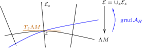
Lemma 3.2.9 (Regularity).
Suppose for some integer . Then any zero of is of class .
Proof.
By the Sobolev embedding theorem we get . By assumption admits a weak derivative of class , say , and almost everywhere. But the RHS, hence , is of class since corresponds to under . Thus the weak derivative is actually the ordinary derivative , hence . More generally, assume for some . Then , hence . Thus the iteration terminates at and shows that . ∎
3.2.2 Arzelà-Ascoli – convergent subsequences
Theorem 3.2.10 (Arzelà-Ascoli Theorem).
Suppose is a compact metric space and is the Banach space of continuous functions on equipped with the sup norm. Then the following is true. A subset of is pre-compact if and only if the family is equicontinuous181818 such that whenever and . and pointwise bounded191919 for every . .
For a proof see e.g. [Rud91, Thm. A.5]. The theorem generalizes to functions taking values in a metric space.
Exercise 3.2.11.
Suppose is a metric space
and is a constant.
a) Show that any family of Lipschitz continuous
functions on with Lipschitz constant
is equicontinuous.
b) Show that any family of differentiable
functions on a closed manifold
whose derivative is bounded by
is equicontinuous.
Further examples of equicontinuous families are provided by -Hölder continuous functions. In practice one often encounters families of weakly differentiable functions on a compact manifold that are uniformly bounded in some Sobolev space . If where then these functions are -Hölder continuous by the Sobolev embedding theorem which applies by compactness of .
3.2.3 Hessian
A Hessian is usually the second derivative of a function or, more generally, of a section of a vector bundle at a point in the domain. However, this is in general only well defined at a critical point, respectively a zero. To extend the concept to general points one chooses a connection or, equivalently, a family of horizontal subspaces. Furthermore, it is often convenient to express the Hessian bilinear form via an inner product as a linear operator, the Hessian operator.
Our setting is the following. Given a symplectic manifold and a Hamiltonian , pick a family of -compatible almost complex structures and denote by the associated family of Riemannian metrics on . At each time consider the corresponding Levi-Civita connection with exponential map and parallel transport along the curve .202020 To easy notation we write and and so on. But we keep indicating time dependence of quantities which involve perturbation at some stage, such as and . Given a vector field along an arbitrary loop ,212121 We assume tacitly that is smaller than the injectivity radius of at . set
to obtain a loop in homotopic to through .
Now consider the map between Banach spaces defined near the origin by
| (3.2.13) |
Since a vector field is in particular of class , there is the natural inclusion which suggests to view this linearization as an unbounded operator with dense domain. The derivative at the origin defines the covariant Hessian operator of , namely
| (3.2.14) |
at any loop .
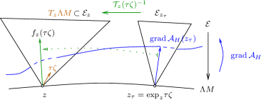
Exercise 3.2.12.
Check that is indeed given by (3.2.14).
Show that is symmetric and even self-adjoint with
compact resolvent. Conclude that the eigenvalues of are
real, accumulate only at , and the eigenspaces
are of finite dimension. Show that .
[Hints: For symmetry see Exercise 2.2.3.
Self-adjointness is a regularity problem.
For compact resolvent see \citerefFH[§2.3]weber:2002a.
To estimate see (3.2.15).
]
The eigenvalues of are real by self-adjointness. Let be a critical point of the symplectic action . Observe that represents the Hessian of at the zero of the gradient. The critical point is called non-degenerate if zero is not an eigenvalue of the Hessian . By self-adjointness of a critical point is non-degenerate iff is surjective. Below after having picked a trivialization we shall say more about the spectrum. A Morse function is a function all of whose critical points are non-degenerate. A Hamiltonian is a regular Hamiltonian if is Morse.
Exercise 3.2.13.
Given , then z is non-degenerate as a critical point iff is surjective iff is non-degenerate as a -periodic trajectory; see (2.3.23).
Lemma 3.2.14.
A non-degenerate critical point of is isolated.
Proof v1..
The critical points of near are in bijection with the zeroes near the origin of the map given by (3.2.13) and corresponds to the origin. But no point other than the origin gets mapped to zero, because is a local diffeomorphism near the origin by the inverse function theorem. The latter applies since the linearization is a bijection: It is injective by the non-degeneracy assumption, hence surjective by self-adjointness. ∎
Proof v2..
Recall the bijection from Exercise 2.3.20. Note that already lies in the ’kernel’ of the differential equation (3.2.14) for any . But must close up at time one in order to lie in the kernel of . This happens precisely if is eigenvector of associated to the eigenvalue . Thus there is an isomorphism
| (3.2.15) |
Now recall Exercise 2.3.21. ∎
The Hessian with respect to a unitary trivialization
Given a loop , pick a unitary trivialization (2.2.8) of the symplectic vector bundle , namely a smooth family of vector space isomorphisms intertwining the Hermitian triples and ; cf. (1.0.9). Conjugation transforms the Hessian into the unbounded linear operator on with dense domain given by
| (3.2.16) |
where is a -periodic family of symmetric matrizes (Exercise 3.2.12), namely
| (3.2.17) |
Example 3.2.15 (Infinite Morse index).
The operator on has eigenvectors and eigenvalues , , .
3.2.4 Baire’s category theorem – genericity
Since the notions surrounding Baire’s category theorem are easily confused, we enlist them for definiteness in more detail than needed here. However, all you should take with you in Section 3.2.4 is Baire’s category Theorem 3.2.18 part (C) and its first application Theorem 3.2.22 ( Morse for generic ).
A topological space consists of a set
together with a collection222222
It is often useful to call a set alternatively a
collection or a family.
Indeed isn’t a “collection of sets” so much easier to absorb than
a “set of sets”?
of subsets
subject to certain axioms.232323
Axioms: The collection , firstly, must contain the empty set
and itself and, secondly, it must be closed under
finite intersections and, thirdly, under arbitrary unions.
Such collection
is called a topology on
.
The
elements are called the open subsets
of the topology, their
complements the
closed subsets.
We often denote a topological space by the shorter symbol
with the understanding that denotes the collection
of open sets – the set being given implicitly as
the largest one of them, the union of all open sets.
A subset of a topological space
is called dense
if it meets (intersects) every non-empty open set or, equivalently,
if its closure contains every point.
A subset of a topological space
is called nowhere dense
if its closure has empty interior, that is
if there is no open set in which is dense:
For each non-empty open set
there is a non-empty open subset
disjoint from .242424
Equivalently, the closure of a nowhere dense set
has a dense complement. Equivalently, the complement
of a nowhere dense set is a set with dense interior.
(Not every dense set has a nowhere dense complement.)
Any countable union of nowhere dense subsets is called
a
meager subset 252525
A meager subset, although a union of nowhere dense sets,
can be dense: Consider .
(alternatively, a subset of the first category in the sense of Baire).
All other subsets, that is all non-meager subsets, are said to be
of the second category in the sense of Baire.
These are somewhere dense.
As first readings we recommend the Wikipedia article
Meagre set,
the online handout
The Baire category theorem and its consequences,
the Blog
The Baire category theorem and its Banach space consequences,
and of [Oxt80].
Exercise 3.2.16.
The subcollection of meager subsets is a -ideal of subsets: Subsets of a meager set are meager, countable unions of meager sets are meager. [Hint: Countable unions of countable unions are countable.]
How about the complements of meager subsets ? These are called residual subsets or co-meager subsets. Let’s call them residuals. Let be the set of residuals. Can the complement of a meager set be meager? Or is it always non-meager, i.e. of the second category?
Exercise 3.2.17.
Suppose and are subsets of a topological space , show:
-
(i)
open and dense complement closed and nowhere dense;
-
(ii)
residual meager countable intersect. of dense open sets;
-
(iii)
Countable intersections of residuals are residuals.
[Hint: (i) Interior . (ii) ’’ Families de Morgan [Kel55, Thm. 0.3]. ’’ Suffices to show: Complement is contained in a meager set.]
Complete metric spaces
A metric space comes with a natural topology , called the metric topology, where the collection of open sets consists of the family of open balls about the points of and arbitrary unions of such. A subset of a metric space is dense if and only if every point of is the limit of a sequence in .
Theorem 3.2.18 (Baire category theorem).
In a complete metric space
-
(A)
meager sets (countable unions of nowhere dense sets) have empty interior;
-
(B)
the complement of any meager set is dense, that is residual sets are dense;
-
(C)
countable intersections of dense open sets, therefore residuals, are dense.
Exercise 3.2.19.
Show that the three assertions (A), (B), (C) are equivalent.
[Hint: Take complements.]
By the exercise it suffices to prove part (C) of the theorem.262626 For a proof see e.g. [Rud91, Thm. 2.2] or [Kel55, Thm. 6.34] or [Oxt80, Thm. 9.1]. See also [KN76, §9] and for references to the original papers see [RS80, Notes to Ch. III]. Concerning a slightly different direction see Remark 3.2.25. In applications one often gets away with a weaker form of the Baire theorem (replace ’dense’ by ’non-empty’):
Corollary 3.2.20 (Baire category theorem – weak form).
For a non-empty complete metric space the following is true.
-
(b)
One cannot write as a countable union of nowhere dense sets.
(A non-empty complete metric space is non-meager in itself.) -
()
If is written as a countable union of closed sets, then at least one of them has non-empty interior.
-
(c)
Countable intersections of dense open sets are non-empty.
So in a non-empty complete metric space, any set with non-empty interior is of the second category (non-meager) by (A). Moreover, the complement of a meager set cannot be meager: Otherwise contradicting (b). Thus which answers the introductory questions and is illustrated by Figure 3.5.
Note that the properties nowhere dense, dense, and somewhere dense do not correspond to the sets , , and . While all elements of are dense subsets of and all nowhere dense subsets are located in , it is possible that even dense subsets are elements of , e.g. .
Remark 3.2.21 (Warning).
Obviously, not all subsets of the second category are dense. For example, the non-dense subset is of the second category: It is not meager since its complement is not dense. In view of this, the in the literature not uncommon wording “every set of the second category is dense by Baire’s category theorem” is rather misleading, often based on defining the sets of the second category as those that contain countable intersections of dense open sets, that is on confusing second category and residual.
Genericity
It is common to call a property P generic if it is ’achievable by small perturbation’. More precisely, in our context a generic property is one that is true for the elements of the set of residual subsets of a complete metric space . In this case the property is shared by the elements of a dense set. In other words, by a small perturbation of an arbitrary pick one can get the desired property.272727 Saying “pick a generic element of ” actually means that one chooses .
Non-degeneracy is a generic property
Theorem 3.2.22 ( Morse for generic ).
Let be a closed symplectic manifold. Then there is a dense open subset of the complete metric space such that the symplectic action functional is Morse whenever .
The proof, given in Example 3.3.32 below, will serve to illustrate abstract Thom-Smale transversality theory (Section 3.3.4) in a simple setting.
Definition 3.2.23 (Non-degenerate case, Morse-regular Hamiltonians).
The terminology non-degenerate case refers to the situation , that is all -periodic orbits are non-degenerate, that is is Morse. Call the elements of Morse-regular or M-regular Hamiltonians.
Proposition 3.2.24 (Finite set).
Given a closed symplectic manifold and an M-regular Hamiltonian , then is a finite set.
Variant: Metrizable complete topological vector spaces
A pair is called a topological vector space if it consists of a vector space together with a Hausdorff 282828 Hausdorff means that any two distinct points are separable by open sets (there are two disjoint open sets such that each of them contains precisely one of the two points). topology for which the vector space operations are continuous. Examples are normed vector spaces. A sequence is called a Cauchy sequence if each open neighborhood of contains the difference for all sufficiently large. If every Cauchy sequence converges to an element , then is called a complete topological vector space. We recommend the concise presentation [Zim90, §1.1].
A topological space is called a Baire space, or simply Baire, if countable intersections of dense open sets, hence residuals, are dense. Examples are complete metric spaces, for instance Banach spaces, hence Banach manifolds.
Remark 3.2.25.
Complete topological vector spaces which are metrizable292929 A topological space is called metrizable if it admits a metric whose open balls generate the given topology, that is every open set is a union of such balls. are Baire spaces; for details of the proof see e.g. [Inf16, Prop. 1.1.8 (B’)]. Theorem 3.2.18 part (C) holds for metrizable complete topological vector spaces.
3.3 Downward gradient equation
Throughout is a closed symplectic manifold. To emphasize time dependence we denote time -periodic Hamiltonians by . Let
| (3.3.19) |
be a -periodic family of -compatible almost complex structures with associated -periodic families of Riemannian metrics and Levi-Civita connections . Let be the space of free contractible loops in and the set of -periodic contractible trajectories of the Hamiltonian flow given by (2.3.19).
As we indicated in Remark 3.2.8 the initial value problem of the gradient is ill-posed on the loop space, no matter which Hilbert or Banach completion one takes into consideration; see also Remark 3.2.4. The way out is to interpret a curve in the loop space asymptotic to critical points as a cylinder in and the formal downward gradient equation on as a PDE for the cylinder in the manifold with asymptotic boundary conditions given by the two -periodic orbits . The key property that makes the analysis work is non-degeneracy of the critical points : This assumption leads to a Fredholm problem, hence to solution spaces of finite dimension. In Section 3.3 we follow mainly \citerefFHsalamon:1999a,Floer:1995a and [HZ11, §6.5].
3.3.1 Connecting trajectories
Fix as in (3.3.19). Pick , that is the functional is Morse, so its critical points are isolated. A smooth map , , is called a trajectory or a Floer cylinder if it satisfies the perturbed non-linear Cauchy-Riemann type elliptic PDE, also called Floer’s equation, given by
| (3.3.20) |
Here denotes the loop , for the gradient see (3.2.12). Floer’s equation generalizes three theories, as indicated in Figure 3.6.
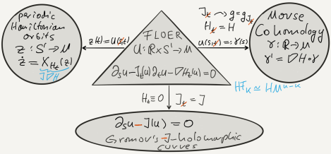
For and the set of connecting trajectories or the connecting manifold303030 Although at this stage is not yet a manifold. or the moduli space of connecting solutions
| (3.3.21) |
consists of all Floer cylinders with asymptotic limits
| (3.3.22) |
where the convergence is uniform in , in other words in .
Remark 3.3.1 (Asymptotic convergence: versus ).
Only asking convergence in the boundary condition of a connecting trajectory may come as a surprise, given that the natural domain of the symplectic action functional is the Banach manifold of loops in . For instance, one would expect that the energy of a connecting trajectory is the difference of the action values of the two asymptotic boundary conditions whenever the asymptotic convergence happens with respect to the functional’s natural topology, in this case . However, Lemma 3.3.2 below shows that asymptotic convergence (3.3.22) is already sufficient to enforce finite energy of . But is this really that surprising? 313131 As the gradient does not generate a flow, the cylinder substitutes are already special to start with. Secondly, being solutions to a PDE, as opposed to an ODE, they are rather exotic, hence rare, creatures. But from exceptional objects one may expect exceptional behavior. Indeed, together with non-degeneracy of the boundary conditions , Theorem 3.3.5 below guarantees even exponential convergence – based on just a convergence assumption, but not to forget that solves an elliptic PDE..
Energy
A useful notion concerning gradient type equations is the energy of arbitrary paths, that is arbitrary cylinders in in our case. It is defined by
| (3.3.23) |
for any smooth cylinder and where the integrand is evaluated at , of course. Note the following.
-
•
The energy vanishes precisely on the periodic orbits viewed as constant trajectories .
-
•
The energy of a trajectory is the square of the norm, namely
(3.3.24) - •
Lemma 3.3.2 (Connecting trajectories are of finite energy).
Given a connecting trajectory , non-degeneracy of is actually not needed, then323232 By definition , mind that the order of in must be the same as of when inserted into .
| (3.3.25) |
Proof.
By (3.3.24) and the gradient nature of the Floer equation we obtain that
To obtain the final step we fixed an extension of
. Then we chose the extensions of the loops
and required by the definition of
by simply connecting these loops along the cylinder to and
its spanning disk .
In the difference each of the integrals
and
appears twice, but with opposite signs.
Because the difference is uniformly bounded from above,
the limit as exists and
is given by the RHS of the first identity
in (3.3.25);
here convergence (3.3.22) enters.
The second identity in (3.3.25)
holds by the earlier argument: Given an extension of the loop choose the natural extension of .
∎
Remark 3.3.3 (Circumventing non-boundedness of – finite energy).
To construct a Morse complex one needs that the trajectories used to define the boundary operator have precisely one critical point sitting asymptotically at each of the two ends. In our case, suppose is a trajectory, how can we guarantee existence of asymptotic limits ? Well, if they exist, the energy identity (3.3.26) shows that is of finite energy. Indeed it turns out, see Theorem 3.3.5, that finite energy of a trajectory is sufficient to enforce existence of asymptotic limits – under the assumption that our functional is Morse. This is why we pick in Section 3.3.
Exercise 3.3.4.
Any smooth cylinder subject to the asymptotic boundary conditions (3.3.22), whether are non-degenerate or not, satisfies the identity
| (3.3.26) |
[Hint: Start at the integral term in (3.3.26). Permute the integrals, so the integral over becomes the inner product of with itself. Use the gradient nature of the Floer equation to end up with which is equal to , as shown in the proof of Lemma 3.3.2.]
Finite energy trajectories
Consider the set of finite energy trajectories
If is Morse, then by Theorem 3.3.5 below every finite energy trajectory is connecting and this non-trivial fact contributes the inclusion in the identity
| (3.3.27) |
The other inclusion already holds without the Morse assumption by (3.3.25). In the non-degenerate case, still assuming that and vanish over , counting with appropriate signs the 1-dimensional components appearing on the RHS of (3.3.27) defines the Floer boundary operator. In the special case of an autonomous small Morse function , see Proposition 2.3.16, and autonomous , the count defines the Morse boundary operator and the RHS of (3.3.27) is naturally homeomorphic to itself. Consequently Floer homology represents the singular integral co/homology of .333333 As is closed and automatically orientable, Poincaré duality identifies . These remarks show the significance of
Theorem 3.3.5.
Let be a Floer cylinder in the non-degenerate case,343434 That is satisfies the Floer equation (3.3.20) on the closed manifold and . then the following are equivalent.
-
(finite energy)
.
-
(asymp.limits)
There are periodic orbits which are the limits of the family of loops ; see (3.3.22). Moreover, the derivative decays, as , again uniformly in .
-
(exp.decay)
There exist constants such that
at every point of the cylinder .
Outline of proof..
The proof is non-trivial, for details we recommend \citerefFHsalamon:1999a. Roughly speaking, (finite energy), namely by (3.3.24) finiteness of the integral over the whole cylinder , enforces via additivity of the integral with respect to disjoint union of the domain that the integrals over annuli must converge to zero, as . But a mean value inequality for based on a differential inequality of the form provides a pointwise estimate of in terms if the norm over some annulus which does not depend on . Thus converges to zero, as , uniformly in . From this one already concludes existence of a sequence such that converges uniformly to some periodic orbit . But by non-degeneracy all periodic orbits are isolated which implies that any sequence diverging to leads to the same limit; similarly for . One has confirmed (asymptotic limits). But (asymptotic limits) implies (finite energy) by Lemma 3.3.2.
Obviously (exponential decay) immediately leads to (finite energy) by (3.3.24) and explicit integration. Conversely, how (finite energy) leads to (exponential decay) is hard to illustrate, have a look at \citerefFH[§2.7]salamon:1999a. A key observation is that lies in the kernel of the trivialization of the linearized operator , see (3.3.31) and (3.3.35), and that for kernel elements the function satisfies a differential inequality for sufficiently large; this is based on invertibility of the Hessian operators at , hence near . It is here where non-degeneracy of the asymptotic boundary conditions enters. This way one arrives at an version of the desired estimate, namely . Application of the operator to leads to a differential inequality , thus to a mean value inequality for which together with the formerly obtained estimate establishes (exponential decay). ∎
3.3.2 Fredholm theory
For convenience of the reader we enlist some basic notions and tools of Fredholm theory. Concerning details we highly recommend [MS04].
Suppose throughout that are Banach spaces. Denote by the Banach space of bounded linear operators equipped with the operator norm . A bounded linear operator is a Fredholm operator if it has a closed range and finite dimensional kernel and cokernel. The latter is the quotient space . It inherits a Banach space structure from since is closed. The map defined on the space of Fredholm operators by
is called the Fredholm index of .
Theorem 3.3.6 (semi-Fredholm estimate).
Given and a compact operator , suppose there is a constant such that
| (3.3.28) |
for every . Then has closed range and finite dimensional kernel.
Exercise 3.3.7.
Prove the previous theorem. Use it to show openness . [Hint: Concerning finite dimensionality it suffices to show that the unit ball in is compact. Use finite dimension together with the Hahn-Banach theorem to reduce the proof of closed range to the case in which is injective; choose a complement of and replace by . Concerning openness use again finiteness of to define an augmentation of which is injective and has closed range . Apply the open mapping theorem, cf. proof of Lemma 3.3.9, to conclude that the inverse of the bounded linear bijection is continuous.]
Exercise 3.3.8 (Stability properties).
a) Show that the subset is open with respect to the operator norm and the index is locally constant, that is constant on each component. Show that353535 [Hint: Use constant index and the fact that the kernel dimension at most decreases locally, see e.g. \citerefFH[Le. 3.7]weber:2002a, to conclude that if is small.] surjectivity of is an open property with respect to the operator norm as well.
b) A compact operator is a (bounded) linear operator which takes bounded sets to pre-compact sets, that is sets of compact closure. Show that the sum of a Fredholm operator and a compact operator is Fredholm and of the same index.
Lemma 3.3.9.
For a bounded linear operator are equivalent:
-
•
is an injection with closed range.
-
•
There is a constant such that
(3.3.29) for every .
Proof.
’’ By the open mapping theorem363636 The open mapping theorem. A bounded linear surjection between Banach spaces is open. A map is called open if it maps open sets to open sets. the inverse of a bounded linear bijection between Banach spaces is continuous. Now pick where , . ’’ By contradiction the inequality itself shows that . By Theorem 3.3.6 the range of is closed. ∎
Definition 3.3.10.
A complement, often called topological complement, of a closed linear subspace is a closed linear subspace such that .373737 Here denotes the internal direct sum of two closed subspaces which by definition means and . If admits a complement it is a complemented subspace.
Examples of complemented subspaces are finite dimensional subspaces and closed subspaces of finite codimension. In a Hilbert space every closed subspace is complemented. We recommend the book by Brezis [Bre83, II.4].
Definition 3.3.11.
A right inverse of a surjective bounded linear operator is a bounded linear operator such that .
Exercise 3.3.12.
Given a surjective bounded linear operator , then
[Hint: ’’ A natural try is . Use to derive the injectivity estimate (3.3.29) for , so is closed, and to conclude . Writing shows that . ’’ Note that the restriction to the complement is a bounded bijection.]
The previous exercise shows that any surjective Fredholm operator admits a right inverse. This generalizes, see part ii), as follows; for details see e.g. \citerefFHweber:2002a.
Exercise 3.3.13.
Let be Fredholm and . It holds that:
-
i)
The range of the bounded operator
is closed with finite dimensional complement. How about ? Give an example in which is infinite dimensional.
-
ii)
If is surjective, then admits a complement, thus a right inverse. Moreover, the projection , , to the second component is a Fredholm operator with
thus .
Remark 3.3.14 (Non-linear Fredholm theory).
A continuously differentiable map
is a Fredholm map
if the linearization is a Fredholm operator
for every . In this
case
is the
Fredholm index of the Fredholm map .
If is not onto one calls a critical point
of
the
Fredholm map .
For a map of class with ,
Fredholm or not, an element is called a
regular value of if for each pre-image
the linear operator is onto
and admits a right inverse.383838
Any outside the image of , i.e. with empty pre-image
, is a regular value.
Then by the implicit function theorem,
see e.g. [MS04, Thm. A.3.3],
the regular level set
| (3.3.30) |
is a Banach manifold whose tangent spaces are given by the kernels, that is
This result is called the regular value theorem. If is even a Fredholm map, then is finite dimensional and .
Exercise 3.3.15.
a) The Fredholm index of a Fredholm map is well defined.
b) The set of critical points of a Fredholm map is closed.
[Hint: b) Exercise 3.3.8 a).]
3.3.3 Connecting manifolds
Consider a connecting manifold as defined by (3.3.21). Recall that is Morse-regular. In this section we show that it is a smooth manifold for generic Hamiltonian and its dimension is the difference of the canonical Conley-Zehnder indices of .
To start with denote the left hand side of Floer’s equation (3.3.20) by , often denoted by to emphasize its Cauchy-Riemann type nature. Let
denote linearization at a zero . Here is a constant; see Remark 3.3.21. As outlined below, see (3.3.32), the linearized operator is of the form
| (3.3.31) |
for every smooth compactly supported vector field along . Here denotes the covariant Hessian operator (3.2.14) of based at a loop . Actually formula (3.3.31) not only makes sense for , let us allow . The Sobolev spaces and are the closures of the vector space of smooth compactly supported vector fields along with respect to the Sobolev norms
Definition 3.3.16.
Abbreviate . The elements of the set
are called MS-regular Hamiltonians or Morse-Smale Hamiltonians.
Exercise 3.3.17 (Constant connecting trajectories, MS-regular M-regular).
Suppose . Show that every
Hamiltonian loop is non-degenerate,
hence is Morse. This shows that .
[Hint: Consider the constant trajectory .]
Exercise 3.3.18 (Morse-Smale condition).
As indicated in Figure 3.6, if are independent of , then the Floer equation recovers the gradient flow of on the closed Riemannian manifold . Show that in this case the elements of are precisely those Morse functions on which satisfy the Morse-Smale condition, i.e. all stable and unstable manifolds intersect transversely.
The significance of MS-regular Hamiltonians lies in the fact that their connecting manifolds are smooth manifolds, even of finite dimension, as a consequence of the regular value theorem; cf. Remark 3.3.14. However, to apply that theorem, two assumptions need to be verified: Firstly, for zero to be a regular value, the kernel of needs to be complemented; cf. Exercise 3.3.12. Secondly, to get to finite dimension of the kernel has to be finite dimensional. Fredholm operators satisfy both criteria.
Thus, modulo proving that is a Fredholm operator and calculating its Fredholm index, the regular value theorem provides part (ii) of
Theorem 3.3.19 (Connecting manifolds).
Given a closed symplectic manifold and a family of -compatible almost complex structures , then
-
(i)
the set of regular Hamiltonians is a residual of ;
-
(ii)
for any any is a smooth manifold. The dimension of the component of is given by 393939 Do not miss our standing assumptions .
where is the canonical Conley-Zehnder index normalized by (2.1.5).
For the proof of part (i) we refer to \citerefFH[§5]Floer:1995a. It utilizes a tool called Thom-Smale transversality theory, see Section 3.3.4 below. It is crucial that the linearized operator is already Fredholm to start with, but this holds true precisely for Morse-regular Hamiltonians. This explains one reason for our standing assumption . Concerning part (ii) we shall sketch below the proof of the Fredholm property of and the calculation of its Fredholm index denoted by .
Remark 3.3.20 (Critical points unaffected by MS-perturbation).
By \citerefFH[Thm. 5.1 (ii)]Floer:1995a one can approximate a given Morse-regular by MS-regular Hamiltonians which agree with along its (finitely many) -periodic orbits. Thus . In \citerefFH[Rmk. 5.2 (ii)]Floer:1995a it is pointed out that it is an open problem whether it is sufficient to perturb outside some open neighborhood of the images of the -periodic orbits of . This would guarantee equality for large . However, the authors point out that it is possible to perturb the family outside such neighborhood to achieve MS-regularity for the given M-regular Hamiltonian itself, just with respect to a perturbed -periodic family of -compatible structures.
Linearization at general cylinders
When it comes to gluing, in Section 3.4.2, it is necessary to linearize given by (3.3.20) not only at zeroes of , but at more general smooth cylinders . The procedure is completely analogous to the definition of the covariant Hessian (3.2.14), just replace the map in (3.2.13) by the map
| (3.3.32) |
given any cylinder . Here denotes the Banach manifold which, roughly speaking, consists of all continuous cylinders which are locally of Sobolev class404040 Here it is crucial to choose , because in this case implies continuity, so one can work with local coordinate charts on to analyze . and converge asymptotically in a suitable way to the given periodic orbits . Convergence of the elements of must be such that the tangent space coincides with the space of vector fields along ; see \citerefFH[Thm. 5.1]Floer:1995a for details. Note that is a vector field along of class . All these spaces fit together in the form of a Banach space bundle whose fiber over is ; see Figure 3.3 for a similar case. Now is a section of whose regularity depends on the regularity of the function ; which is smooth here. To show that
| (3.3.33) |
is equal to the operator displayed in (3.3.31) one can either utilize local coordinates on or work with global notions.414141 We use the notation of a Fréchet derivative, but define it by Gâteaux derivative . See e.g. [LV03, § 3.1] for these notions and when they coincide. Details of both possibilities can be found in \citesymptop[App. A]weber:1999a in the slightly different context of Section 3.5.
Remark 3.3.21 (The condition ).
Roughly speaking, maps on a -dimensional domain of
Sobolev class are continuous, so one can localize,
and well behaved with respect to relevant compositions and products
whenever ; for details see in [MS04]
the paragraphs prior to Prop. 3.1.9 and App. B,
see also the Blog
or not , that is the question.
For instance, the non-linear Fredholm theory,
see Remark 3.3.14,
requires to equip the domain
of the section in (3.3.20)
with the structure of a differentiable Banach manifold.
Choosing with ,
as we did in the previous remark, does the job
(and is the usually selected option), but
leads into the realm of estimates
which are much harder to obtain than estimates.
Another option would be to choose
and ,
of course , and view as a section of the Hilbert
space bundle .
Unfortunately, this choice brings in higher derivatives.
The Fredholm operator
Consider two (non-degenerate) critical points and suppose that is a connecting trajectory.
Theorem 3.3.22 (Fredholm operator).
By non-degeneracy of the linear operator given by (3.3.31) is Fredholm for and
| (3.3.34) |
To prove the theorem it is convenient to represent by an operator acting on vector fields that take values in .
Trivialization
The connecting trajectory extends continuously from the open cylinder to its compactification , because there are the two periodic orbits sitting at the ends by the asymptotic limit condition (3.3.22). Thus we have in fact a hermitian vector bundle over the compact cylinder-with-boundary . Pick a canonical unitary trivialization according to Proposition 2.2.2. In fact, for ease of notation, let us right away agree to omit any ’bars’ from now on completely. Proceed as in (3.2.16) to represent by the operator
given by
| (3.3.35) |
Here the family of symmetric matrizes is given by replacing in (3.2.17) the loop by the family of loops and by . The only new element is the matrix family which converges to zero, as , uniformly in , because actually stands for and vanishes asymptotically by (asymptotic limits).424242 In fact, for any cylinder asymptotic convergence holds. The bad news is that in general is not symmetric, thereby destroying self-adjointness of . The good news is that only amounts to a compact perturbation of (cf.\citerefFH[Le. 3.18]robbin:1995a), so Fredholm property and index, if any, will not change by Exercise 3.3.8 if we simply ignore (while investigating these two properties).
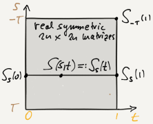
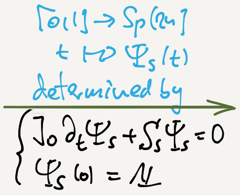
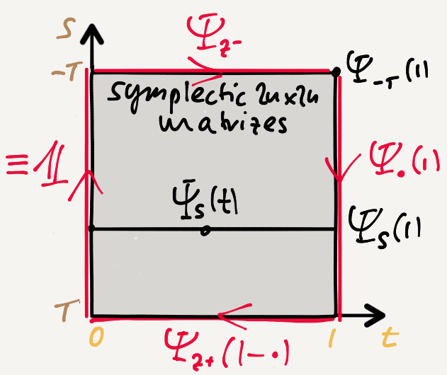
From now on we set . For fixed the path of symmetric matrizes , , determines a symplectic path by
see Figure 3.7 and Exercise 2.1.10. The asymptotic limit matrizes are given by (3.2.17) with and their corresponding symplectic paths lie in : Indeed the paths coincide with the paths in (2.3.24), because they satisfy the same ODE and initial condition, but the latter lie in by non-degeneracy of ; cf. Exercises 2.3.23 and 3.2.13. Thus do admit Conley-Zehnder indices for which we shall choose the canonical normalization (2.1.5), of course. By the uniform limit condition (3.3.22) these indices are actually already shared by the paths whenever is sufficiently large. For simplicity we set
| (3.3.36) |
Fredholm property
We aim to show that the bounded linear operator
in (3.3.35) is Fredholm whenever . To ease notation we shall omit domain and target space in our notation, in general. Pick .
The first step is to establish for the semi-Fredholm estimate (3.3.28) with some suitable compact operator, say the operator
given by composing restriction (continuous) with inclusion (compact for large by \citerefFH[Le. 3.8]robbin:1995a). Details are non-trivial, see \citerefFH[§ 2.3]salamon:1999a. One gets that
for all . The constant depends on the choice of .434343 Here we do linear Fredholm theory. The need for only arises later when we use non-linear Fredholm theory, cf. Remark 3.3.21, to show the manifold property of the spaces of connecting flow lines. The non-linear application is based on the present linear findings. Thus has finite dimensional kernel and closed range by Theorem 3.3.6. Now consider the formal adjoint operator
given by Proposition B.1.3 whose construction is detailed in Appendix B.1.2.444444 The idea is to view as an unbounded operator on with dense domain and construct the unbounded functional analytic adjoint on the dual space with suitably defined domain. Calculate the representative of under the duality isomorphism, notation on . It turns out that ; the inclusion ’’ relies on elliptic regularity. Forget the ambient space of the unbounded operator and interpret . The semi-Fredholm estimate for is equally valid for , just carry out the variable transformation in the integral appearing in the term . Hence has finite dimensional kernel and closed range, as well. The cokernel of is analyzed in Appendix B.1.1 where we introduce the annihilator and show that there are two isometric isomorphisms of Banach spaces, namely
| (3.3.37) |
The first isomorphism is due to the identity (B.1.6) that characterizes , together with restricting the duality isomorphism , to , see (B.1.7), and the second isomorphism is defined by (B.1.2). So
hence . Thus the operator is Fredholm.
Analogously the corresponding two isometric Banach space isomorphisms
| (3.3.38) |
show that . Thus is Fredholm, too.
Fredholm index
Let’s get back to the rectangle worth of symplectic matrizes introduced prior to (3.3.36) and illustrated by Figure 3.7. Let denote the loop of symplectic matrizes obtained by cycling along the rectangle’s boundary once. In \citesymptopRobbin:1993a Robbin and Salamon introduced a Conley-Zehnder type index for rather general symplectic paths in the sense that there are no restrictions on initial and endpoint; see Section 2.1.5. Among the most useful features of the Robbin-Salamon index is that it is additive under concatenations of paths. Furthermore, constant paths have index zero and paths homotopic with fixed endpoints share the same index. Moreover, the Robbin-Salamon index coincides with the Conley Zehnder index () on the set of admissible paths; see Section 2.1.3. Thus
| (3.3.39) |
So to conclude the proof of the index formula (3.3.34) it remains to identify the yet anonymous term in the sum with the Fredholm index of . We relate the unkown term in an intermediate step to another quantity called spectral flow.
The Robbin-Salamon index counts with multiplicities the intersections (called crossings) of a symplectic path with the Maslov cycle in the symplectic linear group . Let us repeat the definition given in \citerefFH[§ 2.4]salamon:1999a that starts from . Slightly perturbing the path, if necessary, leads to finitely many regular crossings , that is crossings at which the following quadratic form is non-degenerate. Suppose that has only regular crossings. The multiplicity at a regular crossing is measured by the signature of the quadratic form
called the crossing form of the symplectic path at . The Robbin-Salamon index, in case there are no crossings at the endpoints, is the sum of signatures
over all crossings. As long as endpoints are fixed, the definition does not depend on perturbations, if any, required to obtain regular crossings.
Recall that by (3.2.15) the domain of the crossing form is isomorphic to the kernel of the unbounded self-adjoint operator on the Hilbert space . Thus in the present context a crossing corresponds to having non-trivial kernel. The quadratic form
is called the crossing form of the family of selfadjoint operators . One can show, see \citerefFH[Le. 2.6]salamon:1999a, that the two crossing forms are isomorphic under the natural isomorphism (3.2.15). Thus the integer
called the spectral flow of the operator family , fits in (3.3.39).
Exercise 3.3.23.
a) Check that the signature of the crossing form
at a regular crossing measures the number of
eigenvalues of , with multiplicities, that change from
negative to positive minus those changing from positive
to negative. So the total change
is a relative Morse index.
b) Suppose the asymptotic operators
have finitely many negative eigenvalues – the number of
which, including multiplicities, is called the
Morse index of and denoted by
. Check that .
To conclude the proof of the index formula (3.3.34) we cite the result in \citerefFH[Thm. 4.21]robbin:1995a that the spectral flow of the family is equal to the Fredholm index of the operator given by (3.3.35).454545 The sign conventions in \citerefFHrobbin:1995a differ from ours in two locations neutralizing each other.
This concludes the (sketch of the) proof of Theorem 3.3.22.
3.3.4 Thom-Smale transversality theory
It happens frequently that one is interested in the set, say , of solutions to some differential equation which depends on some parameter, say a function . Bringing all terms of the differential equation to the same, say left hand, side the problem takes on the form . So we have reformulated as the zero set of a map between suitable spaces. Ideally one hopes that a) zero is a regular value of and b) the linearization of is a Fredholm operator, so that a) the zero set inherits the structure of a manifold whose dimension b) is given by the Fredholm index.
In Section 3.3.4 we will detail the standard technique to achieve this, called Thom-Smale transversality theory.464646 Wassermann \citerefFHWasserman:1969a established equivariant transversality theory in finite dimensions. Example: genericity of Morse-Bott functions; cf. Theorem 5.1.10 in infinite dimensions. We illustrate the theory in Example 3.3.32 by working out the proof of Theorem 3.2.22 which, roughly speaking, asserts that the symplectic action functional is Morse for generic Hamiltonian . In the example we will utilize certain Banach spaces and manifolds whose lengthy constructions we postpone to an appendix at the end of the present Section 3.3.4.
Thom-Smale transversality – abstract theory
From now on and throughout this section suppose is an integer and and are Banach manifolds of class each of which admits a countable atlas and is modeled on a separable474747 A topological space, e.g. a metric space, is called separable if it admits a dense sequence. While non-open subspaces (subsets with induced structure) of separable topological spaces need not be separable (counter-example Sorgenfrey plane), separability of general subspaces holds if either is open or is a separable metric space. Banach space.484848 Such topological spaces and are second countable (topology has countable base), cf. Remark 3.3.28, a property stronger than separable and also called completely separable. Moreover, suppose that
is a Banach space bundle with a section , both of class . Let denote the fiber over . It is convenient to introduce the notation
Recall that the tangent bundle of a vector bundle splits naturally along the zero section. In what follows we use the notation to denote the linearization of a section at a point of the zero section: The (Fréchet) differential composed with projection onto the fiber. For instance, at a zero the linearization is denoted by
and defined by composing the differential
with projection onto the second component . Note that restriction of to yields a bundle of which is a section and with fibers ; similarly with section .494949 To make this precise, consider the inclusion , , and denote the pull-back bundle by ; analogously for . Note also that
| (3.3.40) |
at every zero of .
Theorem 3.3.24 (Thom-Smale transversality).
Let be a section of with
-
(F)
is Fredholm and for each and every .
-
(S)
is surjective, .
Then the subset of the parameter manifold given by
is residual, hence dense, in .
Remark 3.3.25.
In practice, instead of verifying the conditions (F) & (S) for a given section , it is often more convenient to verify the Fredholm condition (F) and the trivial-annihilator condition (A), cf. Appendix B.1.1, namely:
-
(A)
At every zero of the section the annihilator
of the image of the linearization is trivial.
Lemma 3.3.26.
If satisfies (F) & (A), then it satisfies (F) & (S).
Proof.
Suppose . It is a consequence of the geometric form of the Hahn-Banach theorem, see e.g. [Bre11, Thm. 1.7 and Cor. 1.8], that triviality of the annihilator implies density of the image of . (Reversely, density implies triviality by the extension by continuity principle, Exercise B.1.1.) But the image is also closed by Exercise 3.3.13 i). ∎
The proof of Theorem 3.3.24 rests on two pillars. Firstly, the slightly miraculous equality of the set of parameters for which the Fredholm operator is surjective for all and the set of regular values of the projection onto the second component. Secondly, the generalization of Sard’s theorem to infinite dimensions, due to Smale \citerefFHsmale:1965a. Applied locally to , Sard-Smale yields the assertion of Theorem 3.3.24.
Theorem 3.3.27 (Sard-Smale).
Suppose is a separable Banach space and an open connected 505050 If is not connected, simply impose one condition for each component. subset. Let be a Banach space. If is a Fredholm map of class with ,515151 Recall that being a Fredholm map already requires . then the set
of regular values is a residual subset of , thus dense, hence non-empty.525252 However, note that contains any element with empty pre-image .
Remark 3.3.28.
a) The Fredholm condition is necessary; cf. \citerefFHsmale:1965a.
b) Sometimes separability of the target Banach space is added to the assumptions, see e.g. \citerefFHsmale:1965a and [MS04], although seemingly it is not used in the proofs. References without that assumption include [AR67, Cha05].
c) Separability of the domain Banach space
is essential, because the proof uses that separable metric spaces
are Lindelöf
(every open cover admits a countable subcover;
see e.g. [MS04, Prop. A.5.2]).535353
In metric spaces second-countable, separable, and Lindelöf
are three equivalent properties.
To prove the theorem one shows that for every point there is
a closed neighborhood which provides a dense open subset
. One uses Lindelöf to extract a countable
subcover of the collection of all ’s. Then one shows
that ; well explained in [AR67].
By countability of the intersection the Baire Theorem 3.2.18 applies.
d) Banach manifolds: Theorem 3.3.27 extends to Banach manifolds and by applying the Banach space version to local coordinate representations of . Here one adds the assumptions that is modeled on a separable Banach space and that both and can be covered by countably many coordinate charts. In this case can be written as a countable intersection of the dense open sets obtained from the coordinate representations; cf. Step III below.
Proof of Theorem 3.3.24 (Thom-Smale transversality). Suppose is a section with of the Banach space bundle and it satisfies conditions (F) & (S). Let us call a universal section, just to emphasize that and are its restrictions. The proof takes four steps I–IV.
Step I. Suppose and recall the notation from (3.3.40) where is Fredholm from to by assumption (F) and is bounded from to due to . As is surjective by assumption (S), Exercise 3.3.13 ii) asserts that
-
a)
admits a complement, thus a right inverse;
-
b)
projection onto the second component
is a Fredhom operator with .
Step II. Zero is a regular value of by a). Thus by the regular value theorem, see Remark 3.3.14, the universal moduli space, namely the zero set
of the universal section , is a Banach manifold that admits a countable atlas. Moreover, each component of is modeled on a separable Banach space,545454 A finite sum, say , of separable Banach spaces is a separable Banach space and so is any subspace, say . say , and the tangent spaces are given by
Since is a manifold, projection to the second component
| (3.3.41) |
is a map of class . But the linearization of this map at is precisely the Fredholm operator . Thus is a Fredholm map whose Fredholm index along the component of is equal to the index of .
Step III. For each of the countably many local coordinate charts of and of the coordinate representative555555 Here and are the separable Banach spaces on which and are modeled.
of the Fredholm map satisfies the assumptions of the Sard-Smale Theorem 3.3.27. Therefore the set of regular values of is residual in . Hence is residual in the open subset since is a homeomorphism onto its image. Thus the union with the complement of is residual in and represents the regular values of the map . (Recall that elements outside an image are regular values automatically.) The regular values of are those elements of which are regular for all of these maps, that is . But a countable intersection of residuals is residual by Exercise 3.2.17. Thus is residual in the Banach manifold which – being locally modeled on a Banach space – is a Baire space. Hence is dense in .
Step IV. Theorem 3.3.24 is now reduced to the following Wonder-Lemma:
Lemma 3.3.29.
For as in Theorem 3.3.24 the map is defined and
Proof.
Suppose . As the linearization is Fredholm, surjectivity implies existence of a right inverse. Thus it suffices to show
Let us use the notation with ;
see (3.3.40).
’’
Pick , then
for some tangent vector
by the surjectivity assumption (S).
Given , then
by surjectivity of for some element
, that is
. Hence .
’’
Pick , then for some
by surjectivity of .
Thus the pair lies in .
It gets mapped to under .
∎
Thom-Smale transversality – proper implies open
Theorem 3.3.30.
Consider a section satisfying the assumptions of Theorem 3.3.24. Suppose, in addition, that the restriction of the projection , see (3.3.41), to some open subset is a proper map.565656 Proper map: Pre-images of compact sets are compact. Actually the proof only uses that pre-images under of convergent sequences in , limit included, are compact. Then the set of regular parameters
is not only dense but also open in the Banach manifold of all parameters.
Proof.
The set is dense in , as by Theorem 3.3.24 already its subset is.
To prove openness pick and
assume by contradiction that there is no open neighborhood
of in contained in .
Then there is a sequence converging to
and a sequence such that every pair lies in
and the corresponding Fredholm operator
is not surjective.
Consider the compact set that consists of
the convergent sequence together with its limit. The pre-image
is compact by assumption
and it contains the sequence .
Thus there is a convergent subsequence, still denoted by ,
with limit for some . By continuity of the section
the limit of the zeroes also lies in the
zero set .
So the operator is Fredholm by assumption (F)
and it is surjective by our choice .
Recall from Exercise 3.3.8 a) that
surjectivity of is an open property with respect to the
operator norm. On the other hand, the assumption
implies that the partial derivatives
converge to in the operator norm; use local
coordinates about . None of the is surjective. Contradiction.
∎
Given the nice assertion of the theorem, the proof is elementary. This indicates that the hypothesis might be non-trivial to verify in applications.
Morse functions on a closed manifold form an open and dense set
Exercise 3.3.31.
Given a closed manifold , show that the set
of Morse functions on is open and dense in the Banach
space .
[Hint: How about the manifold that consists of constant
maps , for some , and the
map
taking values in ?
Here is the gradient of with respect to any fixed
auxiliary Riemannian metric on .]
Sharpen the exercise by showing that, given a -function and an open neighborhood of in , then is Morse for some -small function supported in .
Symplectic action is Morse for generic Hamiltonian
Example 3.3.32 (Proof of Theorem 3.2.22).
Let be a closed symplectic manifold. Pick a compatible almost complex structure , not depending on time , and let be the associated Riemannian metric and the Levi-Civita connection. Recall that smooth means smooth. Let be the set of all smooth Hamiltonians for which the symplectic action functional , given by (3.2.11) on the space of smooth contractible loops , is Morse. Our goal is to show that is a dense open subset of the complete metric space
| (3.3.42) |
Here the metric is given by (3.2.18) and it is complete.575757 To see that is a metric carry over the arguments in [Inf16, §1.1]. Completeness of follows from the fact that convergence with respect to means convergence with respect to every sup-norm which includes partial derivatives up to order . But is complete since the domain is, firstly, compact by assumption and, secondly, Hausdorff by definition of a manifold; see e.g. Examples 1.1.6 and 1.1.10 in [Zim90]. Now apply Lemma 1.1.14 in [Zim90].
Thom-Smale transversality requires Banach manifolds, so the category is not suitable. As pick the completion of the space with respect to the Sobolev norm; cf. Proposition A.1.4.585858 is the Hilbert manifold of absolutely continuous contractible maps with square integrable derivative . The tangent space consists of absolutely continuous vector fields along with square integrable derivative . As parameter manifold of Hamiltonians we choose the separable Banach space595959 Cf. Proposition A.1.1; compactness of is crucial for completeness of .
| (3.3.43) |
and as section the gradient . Let be the subset whose elements make Morse.
Observe that coincides with the set of regular values of the section that appears in the Thom-Smale transversality Theorem 3.3.24. To see this note that since and since the zeros of , although apriori only of class , automatically inherit -smoothness from by Lemma 3.2.9. Recall that, by Exercise 3.2.13, non-degeneracy of as a critical point of is equivalent to surjectivity of the linear operator that represents the Hessian of at . But since .
To summarize and both definitions
agree. Theorem 3.3.24 will ultimately prove, see Step III, that
| the set is dense and open in for . | (3.3.44) |
Suppose that (3.3.44) has already been established. Then we can approach the smooth scenario through the back door, namely, by approximation:
Density of in . Given a smooth Hamiltonian , viewed as being of class , let us exploit density, in order to -approximate by some as illustrated by Figure 3.8.
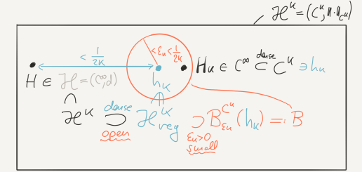
By openness contains a whole open -ball about . Now -approximate by a smooth Hamiltonian using the standard fact that -functions are dense in the Banach space of -functions, see e.g. [Hir76, Thm. 2.6], hence in the open subset . Choosing in each of the two approximation steps a -distance less than we get that for every ; set . At first sight somewhat amazingly, this is already enough to obtain convergence , despite not having any control whatsoever on the higher -norms of that appear in the infinite sum . However, a second look reveals that the weights take care of the higher -norms:
Given , choose the integer sufficiently large such that , then for every integer it holds that . Since each lies in this proves density in of the set of smooth regular Hamiltonians.
Openness of in . Pick . Then by openness (3.3.44) for there is a small radius such that the whole open ball about lies in . Set and pick with
But this inequality implies that and therefore
Thus the whole open ball is contained in . So is open.
I. Setup and Fredholm condition (F). Pick an integer . We apply Thom-Smale transversality theory to these choices: The Banach manifolds
each admits a countable atlas and is modeled on a separable Banach space, see Appendix A.1, and the section given by the gradient
of the symplectic action functional defined by (3.2.11). Here
is the Hilbert bundle whose fiber over consists of the square integrable vector fields along the loop in ; fibers do not depend on . Bundle setup and the calculation of the gradient have been carried out in Section 3.2.1.
Observe that is linear, so together with our previous calculation in Section 3.2.3 of the Hessian of at a critical point , see (3.2.14), we observe that the linearization of at a zero
is given by
| (3.3.45) |
where is given by (3.2.14) and where
Note that
so . By Exercise 3.2.12, as an unbounded operator on with dense domain , the Hessian has a finite dimensional kernel which, by self-adjointness, coincides with the cokernel. As an operator from to the Hessian is bounded, notation , thus a Fredholm operator with .
Hence assumption (F) in Theorem 3.3.24 is satisfied once is of class . But this is readily verified by estimating, based on and after choosing suitable trivializations, firstly, the norm of the difference of and in terms of and, secondly, the norm of the difference of and applied to . The second estimate should be in terms of . Continuity of the two partial derivatives then implies that the derivative of exists at each point and varies continuously itself (in [AP93, Ch. 1] combine Thm. 4.3 with Prop. 4.2).
II. Transversality condition (S). By Lemma 3.3.26 it suffices to verify condition (A): At every zero of the annihilator of the image of is the trivial vector space. In other words, given , we have to show that the two assumptions
together imply that . As usual, the assumption involving the Fredholm operator will improve the regularity of which one then exploits to invalidate the other assumption whenever is not the trivial vector field.
As , assumption one means that , thus by self-adjointness . Hence the vector field is in fact continuous by the Sobolev embedding theorem, see e.g. [MS04, Thm. B.1.11]. From now on suppose by contradiction that
Below we are going to construct an element which has the property that . Contradiction.
The construction of will be local. Let be the injectivity radius of . We utilize coordinates about the point provided by the exponential map and modeled on the radius ball . The tangent space comes with the inner product denoted by . The piece of the loop inside the coordinate patch determines a curve in via the identity .
-
•
As and is continuous, there is a time interval about with
-
•
As and is continuous,606060 Let be the derivative of at . As is invertible, also remains invertible for all near the origin. there is a time interval about with
-
•
With pick a cutoff function as in Figure 3.10. Denote the -periodic extension of to again by .616161 Viewing as a map on such that we may suppose that .
-
•
Pick a cutoff function as in Figure 3.10.
-
•
Define a smooth function with for all by
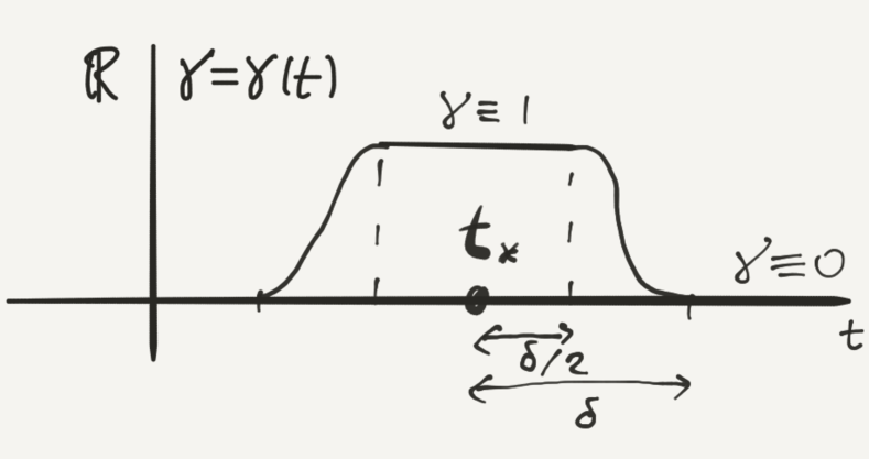
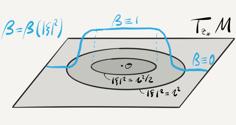
Straightforward calculation shows that
But this is the desired contradiction to assumption two. The second equality holds since for values outside the function is identically zero by definition. Equality three holds since is supported in . Observe that is defined by the overbraced identity; set to get that and apply to both sides to get that .
III. Density and openness in the category. To conclude the proof of Theorem 3.2.22 we show (3.3.44), that is density and openness of in .
Proof of Theorem 3.2.22.
Density: By Steps I and II the Thom-Smale transversality
Theorem 3.3.24 applies to
with .
Openness: By Theorem 3.3.30
it remains to show that the projection in (3.3.41)
is a proper map. The Banach manifold is given by
Properness: Given a compact subset and a sequence in
we need to extract a convergent subsequence (the limit of which then
lies automatically in the zero set by continuity of ).
Observe that the sequence lives in .
Compactness of allows to extract a convergent
subsequence, still denoted by , and a limit .
This has the consequence that the right hand sides of the sequence
of differential equations ,
each being by Lemma 3.2.9,
are well behaved in the sense that they have a continuous limit
if the sequence has one.
By compactness of the sup norm over of the vector field is finite. Hence the families and are pointwise bounded. Since with both families are equicontinuous by Exercise 3.2.11 b). Now apply the Arzelà-Ascoli Theorem 3.2.10 to extract subsequences, without changing the notation, and continuous loops and such that and in . In this case , see e.g. [Zim90, Le. 1.1.14], hence . On the other hand, using the equations, the sequence converges in to the vector field .626262 Set , then , as ; cf. (3.2.13).
Thus we found a subsequence of which admits a limit . The latter inclusion holds since . ∎
This concludes Example 3.3.32.
Classical action is Morse for generic potential
Example 3.3.33.
Given a closed Riemannian manifold , the classical action functional defined by (3.5.58) is Morse for generic smooth potential functions ; for details see \citerefFHweber:2002a. Here the critical sets are not necessarily compact, but there parts in sublevel sets are for each regular value of . Hence Step III above will require refined arguments.
3.4 Floer chain complex and homology
In this section we define the Floer complex associated to a regular pair on a closed symplectic manifold . We only consider the simplest case in which and vanish over ; cf. (3.0.1). The corresponding homology, called Floer homology, transforms by isomorphisms when changing regular pairs and in the end of the day represents, again naturally, the singular homology of . For simplicity we take coefficients in all homology theories in Section 3.4.
Definition 3.4.1.
A regular pair consists of a Hamiltonian , that is a periodic family of functions of functions on , and a periodic family of -compatible almost complex structures such that the following is true: The action functional given by (3.2.11) is Morse and the linearized operators given by (3.3.31) are surjective for all connecting trajectories and all Hamiltonian loops .
Earlier we showed how to obtain a regular pair: To satisfy the Morse condition, pick an element of the residual subset provided by Theorem 3.2.22. Now pick a family of -compatible almost complex structures on . Then, either perturb away from its critical points, see Theorem 3.3.19, or stay with and perturb the family , see \citerefFH[Thm. 5.1]Floer:1995a, to obtain a regular pair denoted by .
Definition 3.4.2.
Pick a regular pair . Then the vector spaces
graded by the canonical, that is clockwise normalized, Conley-Zehnder index,
see (2.1.5) and (2.3.25),
are called the Floer chain groups
associated to the Hamiltonian .
By convention the empty set generates the trivial vector space.
The set of all contractible -periodic
Hamiltonian orbits is finite by Proposition 3.2.24.
The subset of those of index is a basis of
, called the canonical basis (over ).
The Floer boundary operator is given on a basis element by
| (3.4.46) |
where is the number (mod 2) of connecting flow lines.636363 A connecting flow line is an unparametrized solution curve, the image of a flow trajectory , , between two critical points . Connecting flow lines are in bijection with the set of those with . This is a finite set by Exercise 3.4.12. Let be the number of elements modulo 2.
Proposition 3.4.3 (Boundary operator).
It holds that .
Exercise 3.4.4.
Given , show that is equal to the sum over all where the coefficient of each is the number (mod 2) of 1-fold broken flow lines that start at , end at , and pass an intermediate critical point of index at which and meet; cf. footnote.
So to prove it suffices to show that the number of such 1-fold broken flow lines between and is even. To see this one shows that for each there exists precisely one partner pair which is determined by the property that there is a 1-dimensional connected non-compact manifold, i.e. an open interval, of trajectories running straight from to and whose two ends correspond to the two partner pairs; see Figure 3.1. The sense in which the two ends correspond to partner pairs is introduced and detailed in Section 3.4.1 on compactness up to broken flow lines. The gluing procedure developed in Section 3.4.2 excludes that two families converge to the same broken flow line . To summarize, the set of 1-fold broken flow lines from to is in bijection with the ends of finitely many open intervals, so the number of them is even.
Definition 3.4.5.
The chain complex
is called the Floer complex associated to a regular pair . The corresponding homology groups, called Floer homology groups, are graded vector spaces. They are denoted by
Theorem 3.4.6 (Continuation).
For any two regular pairs and there is a natural 646464 Here natural isomorphism means that there are no (further) choices involved. isomorphism
Furthermore, given a third regular pair , then
Theorem 3.4.7 (Calculation).
Suppose is a closed symplectic manifold such that and vanish over . Then for any regular pair there is an isomorphism of degree denoted by
and these isomorphisms are natural in the sense that
Corollary 3.4.8.
The weak non-degenerate Arnol ′d conjecture (1.0.2) is true.
3.4.1 Compactness – bubbling off analysis
Throughout is Morse. Let be the space , see (3.3.21), of connecting trajectories between contractible -periodic orbits .
Definition 3.4.9 (Convergence to broken trajectory).
We say that a sequence of connecting trajectories converges to a -fold broken trajectory656565 or, alternatively, converges to a broken trajectory with components if the following holds true. There are
-
-
pairwise different periodic orbits ,
-
-
(non-constant) connecting trajectories for ,
-
-
sequences of reals for ,
such that the sequence of maps , converges to in , as , i.e. uniformly with all derivatives on compact sets. By
we henceforth denote convergence to a broken trajectory; see Figure 3.11.
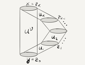
Exercise 3.4.10 (Strictly decreasing index in case of a regular pair).
Show that the index ,
strictly decreases
along the members of a broken trajectory
whenever is a regular pair.
[Hint: By non-constancy each comes in a family
of dimension at least . But this dimension
is a Fredholm index. Now recall (3.3.34).]
Proposition 3.4.11 (Compactness up to broken trajectories).
Suppose is Morse. Then any sequence of connecting trajectories admits a subsequence which converges to a broken trajectory , as .
It is interesting to observe that by, and in the sense of, the proposition the space of finite energy trajectories, see (3.3.27), is compact for a regular pair.
Exercise 3.4.12 (Finite set in case of a regular pair ).
Show that in case of index difference one, that is , the set of those connecting trajectores whose initial loop lies on a fixed intermediate action level, say , is a finite set.666666 The set parametrizes the flow lines from to , in other words, the set of connecting trajectores modulo time shift. As maps and are different, but their image curve in the loop space, i.e. their flow line, is the same.
Proof of Proposition 3.4.11 (Compactness up to broken trajectories)
The proof has four steps the first of which is highly trivial, at least in the present case of a compact manifold . We only sketch the main ideas. Actually the first three steps do not require that is Morse, not even that are non-degenerate. The Morse requirement enters in Step IV through Theorem 3.3.5.
Step I. (Uniform bound for )
Obvious by compactness of .
Step II. (Uniform bound for – bubbling off analysis)
In fact, to carry out Step III below a uniform bound, for some constant , for the sequence of connecting trajectories would be sufficient. Note that we get a uniform bound for free due to the energy identity (3.3.25). But this is not good enough to get uniform bounds; cf. also Remark 3.3.21.
On the positive side, investing some work even leads to a uniform bound, that is
To prove this, assume by contradiction there was a sequence of points along which the derivative explodes, as . It is convenient to view maps defined on likewise as maps on which are 1-periodic in the imaginary part . Exploiting the invariance of under shifts in the variable in order to replace by the shifted sequence and then by compactness of picking a subsequence, we assume without loss of generality that , as . Now there appears yet another Wonder-Lemma, called the Hofer-Lemma [HZ11, §6.4 Le. 5]. When applied for each to the continuous non-negative function on the complete metric space , the point , and the constant , the Hofer-Lemma yields a sequence of points and constants such that
-
•
-
•
-
•
-
•
Note that , so the derivative explodes as well along the new sequence of points which also converges to , but for which we have more information than we had for . The key step is then to consider the sequence of rescaled smooth maps
These maps have the property that they are non-constant and uniformly bounded on balls whose radius tends to infinity. More precisely,
-
•
-
•
on , see Figure 3.12
-
•
Now one shows that there is a smooth map and a subsequence, still denoted by , such that in , that is uniformly with all derivatives on . In view of the Arzelà-Ascoli Theorem 3.2.10 it suffices to establish uniform in bounds on compact sets for and each of its derivatives. In view of the Sobolev embedding theorem, see e.g. [MS04, Thm. B.1.11], it suffices to establish uniform bounds for , that is for each and each compact set find a bound for the restriction to such that serves for all . The key input is the Calderón-Zygmund inequality (3.4.48) for the Cauchy-Riemann operator . The desired bounds are established by induction on . For details see e.g. \citerefFH[Le. 5.2]salamon:1990a, using elliptic bootstraping techniques, or [HZ11, §6.4 Le. 6], using the Gromov trick to first get rid off the Hamiltonian term followed by a proof by contradiction.
The limit map satisfies the equation
| (3.4.47) |
where . The solutions of this elliptic PDE are called -holomorphic planes or pseudo-holomorphic planes. They have been introduced in Gromov’s 1985 landmark paper \citeintrogromov:1985a. Since
we arrive at a contradiction as soon as we can show that extends continuously from to the Riemann sphere, that is to a continuous map . Indeed in this case the proof of Proposition 3.4.11 is complete since
Here the first identity uses that by our standing assumption (C2) the evaluation map of over vanishes, see (3.0.2), and the second identity holds since a point has measure zero.
So it remains to construct the continuous extension . For each radius the map gives rise to a loop in by restriction to the radius- sphere in centered at the origin; notation ; indicated red in Figure 3.12. In \citerefFH[Pf. of Prop. 4.2]salamon:1990a it is shown, see also [HZ11, paragraph before (6.94)], that the lengths of the image circles in of the maps tends to zero, as .
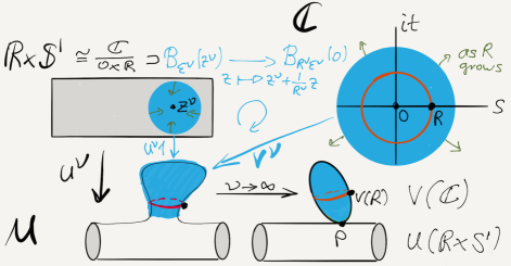
While along any sequence the family of points admits a convergent subsequence by compactness of , continuity of together with the length shrinking property imply uniqueness of the limit and independence of the choice of the sequence . Clearly completes the image to be a 2-sphere and we are done.676767 As lies in the closure of the image of , it lies in the closure of the union of all images . So the bubble is attached at to whatever is the limit, see Step IV, of the ’s.
Step III. (Uniform bound for – elliptic bootstrapping)
First of all, in view of the uniform bound
for our sequence of connecting trajectories ,
obtained in Steps I and II,
the Arzelà-Ascoli Theorem 3.2.10
provides a continuous map
to which some subsequence, still denoted by ,
converges uniformly on compact sets. This allows
to analyze the problem in local coordinates on ,
hence for maps taking values in .
To derive uniform estimates for the sequence
on compact sets is, surely without surprise, an iterative procedure.
To illustrate the basic mechanism behind,
let us incorrectly oversimplify things by assuming
that (i) each is a map ,
, supported in a compact set
– which it clearly isn’t, given the non-linear target
and the asymptotic boundary conditions and –
and that (ii) each satisfies the much simpler PDE
The iteration rests on the Calderón-Zygmund type inequality
| (3.4.48) |
and its immediate consequence (replace by derivatives of )
These hold true for any compactly supported map whenever and and where the constant only depends on ; see e.g. \citerefFH[III §1 Prop. 4]Stein:1970a or \citerefCG[Thm. 2.6.1]Wendl:2015a. By continuity the estimates continue to hold for in the closure of with respect to the norm.
Application to our oversimplified maps shows that
where the constant does not depend on . More precisely, starting with we get a uniform bound on which then leads to a uniform bound and so on for every . The Sobolev embedding theorem, see e.g. [MS04, Thm. B.1.11], then provides uniform bounds on for every . Now apply the Arzelà-Ascoli Theorem 3.2.10 to each derivative of .
However, the general case is much harder, of course, mainly due to the non-linearity in front of the highest order term . The fact that the maps are not of compact support at all, requires the use of cutoff functions leading to additional terms as well. For details see e.g. [HZ11, §6.4 Le. 6] or \citerefFH[Le. 5.2]salamon:1990a.
Step IV. (The limit broken trajectory)
Pick and consider the restrictions of to . By Step III there are uniform bounds for on , thus there is a subsequence, still denoted by converging uniformly with all derivatives to some smooth map which solves the Floer equation (3.6) as well. Replacing by and choosing subsequences if necessary one concludes that restricted to converges to a smooth solution which coincides with on . Iteration leads to a smooth limit solution again denoted by . If we knew that was of finite energy we would apply Theorem 3.3.5 to obtain existence of periodic orbits sitting at the ends of , that is . With this understood apply the finite686868 The downward procedure can only end at and it ends after at most many steps: The action strictly decreases from to iff iff , but there are only finitely many periodic orbits by Proposition 3.2.24. iteration detailed in \citerefFH[Pf. of Prop. 4.2]salamon:1990a to get the desired limit broken trajectory .
Let us check that the energy of the limit solution is indeed finite. By the energy identity (3.3.25) for connecting trajectories we get
where and the last identity is true since is the downward gradient of . By uniform convergence we can take the limit over to get the estimate
| (3.4.49) |
for every , in particular, for . Thus .696969 The case for every is not excluded: Given , consider the upward shifts . So and . Then and both converge to , as . Indeed on compact sets converges uniformly with all derivatives to the constant trajectory .
This concludes the proof of Step IV and Proposition 3.4.11.
3.4.2 Gluing
Suppose is a regular pair and pick periodic orbits of -indices , respectively. To conclude the proof of Proposition 3.4.3 () let us construct a continuous map707070 Warning. Here denotes the true zero, in \citerefFH[§3.4]salamon:1999a the approximate zero .
called the gluing map, whose image lies in one component of the 1-dimensional manifold of which it covers one ’end’ in the sense that , as . In other words, the broken trajectory represents the boundary point of that end. Furthermore, and most importantly, as it concludes the proof of , no sequence in , that is no sequence away from the image of the glued family , converges to ; see Figure 3.13.
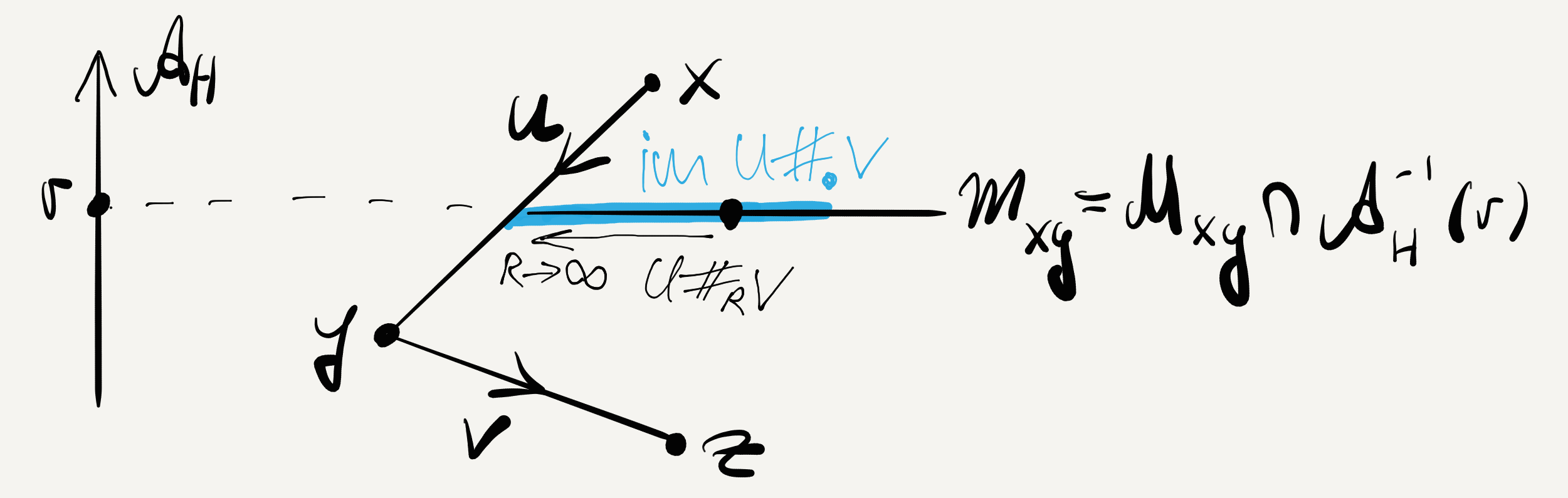
The construction is by the Newton method to find a zero of a map near a given approximate zero : Roughly speaking, one needs that is ’small’, the derivative at is ’steep’,717171 More precisely, in our context needs to admit a uniformly bounded right inverse . and does not vary ’too much’ near the approximate zero; see Figure 3.14.
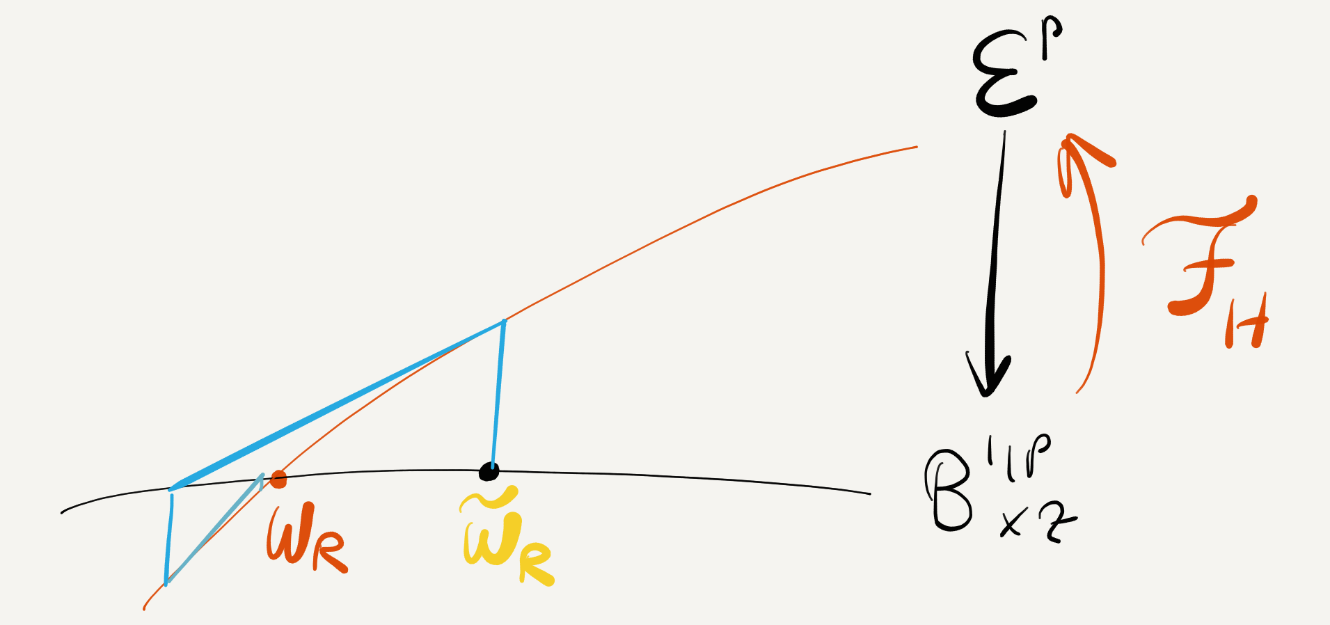
We only outline the construction and refer to \citerefFH[§3.3]salamon:1999a for details. Obviously is the Floer section (3.3.20) of the Banach bundle ; cf. (3.3.32). To start with pick and and consider the approximate zero used in \citerefFHsalamon:1999a and illustrated by Figure 3.15. Next, as we wish to use the implicit function theorem, we need to move from Banach bundles to Banach spaces. So, we replace by the map
where denotes parallel transport; cf. (3.2.13) and (3.3.32).
Exercise 3.4.13.
a) The map is
a bijection between the zeroes of and those of .
b) The linearization
is .
[Hint: Compare \citesymptop[Pf. of Thm. A.3.1]weber:1999a.]
So the tasks at hand are to
-
(a)
show that admits a unique zero whenever is sufficiently large;
-
(b)
show that , as ;
-
(c)
define .
Obviously we start with task (c). Next, concerning task (b), let us argue geometrically by looking at Figure 3.15 where is a cutoff function that equals zero for and one for . Observe that the curve follows more and more, the larger , all of and all of . Thus restricted to a fixed compact subdomain, say of the form , runs into the constant in solution , unless it is shifted appropriately backward or forward in in which case it runs towards a piece of or , respectively.
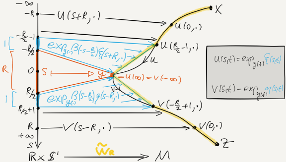
Concerning task (a) let us discuss informally the three ingredients needed to carry out Newton’s method.
I. Approximate zero. The norm of , hence of since parallel transport is an isometry, is equal to the norm of applied to the parts of along the length 1 domain and an analogous length 1 domain in the positive half cylinder. Let us pick the -piece of to illustrate what happens.727272 Concerning the other piece of , check how applied to approaches , as . The derivative is a sum of two terms: Term one approaches zero, as , since approaches uniformly in and term two approaches zero, as , since does. By (exp. decay) in Theorem 3.3.5 both terms converge to exponentially, as . So the integral over the length 1 interval – which moves to with – becomes as small as desired by picking large.
II. Right inverse. By assumption both Fredholm operators and , see (3.3.31), are surjective. Salamon proves in \citerefFH[Prop. 3.9]salamon:1999a that there are constants and such that for any the Fredholm operator based on the approximate zero is surjective as well and, moreover, there is an injectivity estimate for on the range of , namely
for every . It is, of course, crucial that the estimate is uniform in .
Exercise 3.4.14.
Suppose . (i) Show that is a bijection and admits a continuous inverse. (ii) Show that
is a right inverse of and calculate its operator norm. [Hint: Recall (3.3.38).]
III. Quadratic estimates. To see what is meant by quadratic estimates have a look at \citerefFH[Prop. 4.5]salamon:2006a.
With all three preparations I-III in place, apply to the implicit function theorem in the form of \citerefFH[Prop. A.3.4]salamon:2006a with to obtain a unique such that , equivalently, such that where
This concludes the construction of the gluing map and thereby the proof of Proposition 3.4.3 ().
3.4.3 Continuation
Suppose throughout that is fixed and that , , and are regular pairs.737373 E.g. pick three elements of the set provided by Theorem 3.3.19. By or we denote a homotopy between Hamiltonians, that is a smooth map such that
The key idea is to replace the -independent Hamiltonians in the Floer equation (3.3.20) by -dependent homotopies, thereby destroying the occasionally disturbing symmetry under -shifts; see footnote to (3.4.49). Consider the PDE
| (3.4.50) |
for smooth cylinders . It is called the homotopy Floer equation and its solutions homotopy trajectories. Impose the usual asymptotic boundary conditions (3.3.22) for two periodic orbits and of different Hamiltonians and denote the set of such by
Just as before, for a generic, called regular, homotopy this moduli space is a smooth manifold for any choice of and the dimension is the index difference . There are also analogous compactness and gluing properties. The difference is that due to the missing invariance under shifts in the -variable one uses the index difference zero moduli spaces (compact, thus finite, sets) to define maps which are given on by
| (3.4.51) |
The index difference one moduli spaces lead to the chain map property
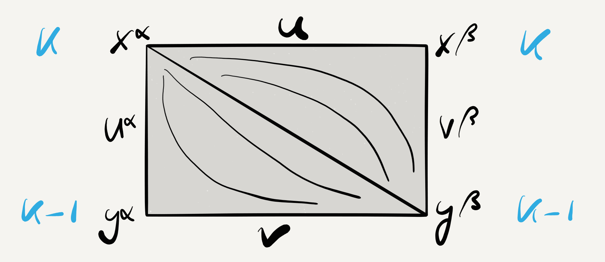
This identity is equivalent to all 1-fold broken trajectories from to appearing as partner pairs as indicated by Figure 3.16. Just as before the partner pair property follows from compactness up to 1-fold broken orbits and a corresponding gluing construction. The induced morphism on homology
| (3.4.52) |
is called Floer continuation map. Does it depend on the homotopy?
Exercise 3.4.15.
Denote the constant homotopy again by for simplicity. Show that is the identity on .
Lemma 3.4.16 (Salamon \citerefFH[Le. 3.11]salamon:1999a).
Given regular homotopies from to and from to , define a map
where is a constant; see Figure 3.17. Then there is a constant such that for the map is a regular homotopy from to and the induced morphism
is given by
| (3.4.53) |
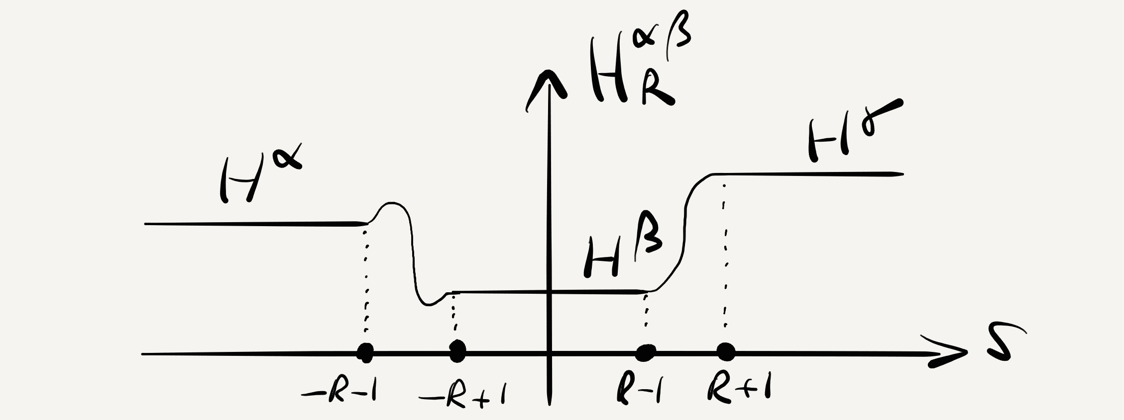
Exercise 3.4.17 (Continuation maps independent of homotopy).
Given two regular homotopies and from to , show that and are chain homotopy equivalent: Define a homomorphism
such that
| (3.4.54) |
Note that such raises the grading by .
[Hint: Pick a regular homotopy of
homotopies
from to which agrees with
for and with for .
In case of index difference the
parametrized moduli
spaces
are 0-dimensional manifolds, in fact finite sets. Count them appropriately to define . Analyze compactness up to 1-fold broken orbits of the (1-dimensional) index difference moduli spaces and set up corresponding gluing maps to prove the desired identity (3.4.54); cf. \citerefFH[Pf. of Le. 3.12]salamon:1999a.]
Proof of Theorem 3.4.6 (Continuation)
To prove that is an isomorphism with inverse pick a regular homotopy from to and denote the (regular) reverse homotopy by . With the associated homotopy of Lemma 3.4.16 we get
where identity two is by (3.4.54) for the two regular homotopies and from to itself. Identity three is by Exercise 3.4.15. Hence . Repeat the argument starting with a homotopy from to to get . This shows that is an isomorphism with inverse . That follows from Exercises 3.4.15 and 3.4.17. The identity holds by (3.4.53). This proves Theorem 3.4.6.
3.4.4 Isomorphism to singular homology
Recall that we use coefficients. After introducing in great length a new homology theory for the data – which does not depend on as we saw in the previous section on continuation – it is natural to ask if Floer homology relates to any known homology theory and if so, how? The answer is that Floer homology relates to singular homology of the closed manifold itself by isomorphisms compatible with the continuation maps .
Method 1 ( small Morse functions)
Floer observed in \citerefFH[Thm. 2]floer:1989c that, roughly speaking, if one chooses a sufficiently small Morse function as Hamiltonian, then not only the -periodic orbits of are precisely its critical points, see Proposition 2.3.16, but also the connecting Floer trajectories will not depend on and turn into connecting Morse trajectories .
Remark 3.4.18 ( small: Floer trajectories reduce to Morse – not always!).
Actually the situation is a bit more complex as we said right above: Hofer and Salamon proved in \citerefFH[§7]Hofer:1995a that for sufficiently small Morse functions all connecting trajectories of index difference one or less are independent of and therefore connecting Morse trajectories. But index difference one (and zero) is all that is needed in either chain complex. (See \citerefFH[Ex. 7.2]Hofer:1995a for an example how -independence fails in case of index difference two or larger. See also \citerefFH[Rmk. 7.5]Hofer:1995a saying that their proof does not work for symplectic manifolds of minimal Chern number .)
Suppose from now on that is Morse and small. A closer look shows that the Floer equation (3.3.20) actually turns for -independent trajectories into the upward gradient equation
| (3.4.55) |
for curves ; cf. Figure 3.6. Note that by Proposition 2.3.16 and that along the critical set. Furthermore, by (2.3.26) the Floer grading as a constant periodic orbit and the Morse index of as a critical point of are related by .
Recall from Section 3.1.2, see [Web] for details, that the Morse cochain groups of a Morse function on a closed manifold are generated by the critical points of , graded by their Morse index , and the coboundary operator is given by counting the flow lines of the upward gradient , that is from critical points of index, say , equivalently to those of index , equivalently .
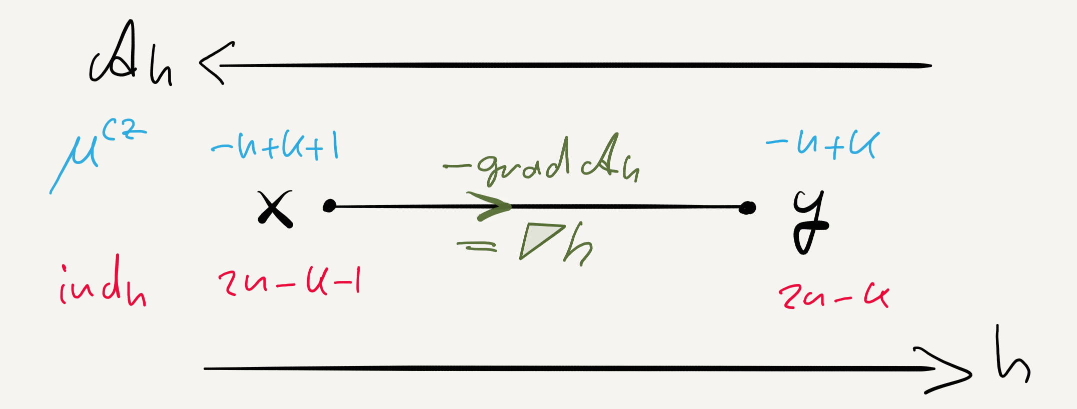
Note that by (3.4.55). Consequently for any sufficiently small Morse function, denoted for distinction by
the following chain and cochain complexes are naturally equal
| (3.4.56) |
up to shifting the grading, that is is naturally equal to .
To prove Theorem 3.4.7 consider a regular pair and define the desired isomorphism, say denoted by , by composing the following three isomorphisms: Firstly, the Floer continuation map
for some small Morse function . Secondly, the isomorphism
induced by the chain level identity (3.4.56), followed by Poincaré duality747474 Any symplectic manifold is naturally oriented and our is closed by assumption.
Thirdly, the fundamental isomorphism (3.1.5) of Morse homology given by
and compatible with the Morse continuation maps. We use coefficients.
Method 2 (Spiked disks –PSS isomorphism)
Piunikhin, Salamon, and Schwarz came up in \citerefFHPiunikhin:1996a with a rather different idea to construct an isomorphism between Floer and Morse homology, denoted by
Fix a Morse function and a (generic) Riemannian metric on such that the Morse complex is defined and pick a generator . Suppose is a regular pair, so Floer homology is defined, and pick a generator . The idea is to relate Morse and Floer flow lines by first following a Morse flow line that comes from and then, say at time , change over to a Floer flow line that goes to . Of course, the transition from a family of points to a family of circles requires some interpolation, i.e. some thought. The idea is to look at -holomorphic planes , see (3.4.47), and homotop, as the polar radius of points in traverses the interval , the zero Hamiltonian inside the unit circle (polar radius ) to the given Hamiltonian on and outside the circle of polar radius . Denote such a homotopy by . Moreover, one requires to converge to the given periodic orbit , as . The key condition that couples the two worlds is then that meets at . Such a configuration, called a spiked disk, is illustrated by Figure 3.19.
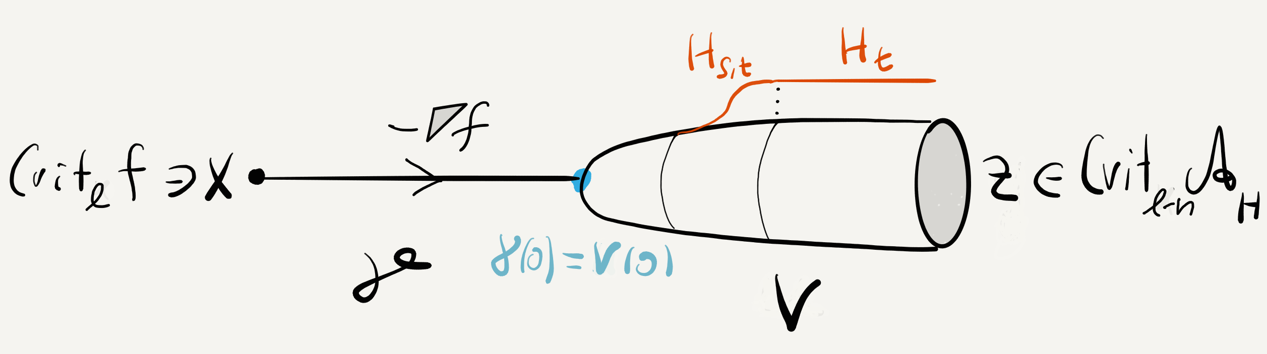
Now the codimension of the set of all possible points is . And the set of all which satisfy the homotopy Floer equation (3.4.50) for and converge to , as , has dimension .757575 The dimension formula in \citerefFH[§ 3.5]salamon:1999a involves . Thus the moduli space of spiked disks is (for generic homotopy ) a 0-dimensional manifold in case the Morse index of is equal to . Also there is ’no index left’ for broken flow lines, so one has compactness, thus finiteness of index difference zero moduli spaces. It is now clear that on the chain level the homomorphism
is defined by counting (modulo 2) the finitely many spiked disks from to . The index difference one moduli spaces are compact up to 1-fold broken orbits, the breaking can happen on either side, which together with a gluing construction shows that the 1-fold broken orbits come in pairs, namely as partner pairs. This shows that is a chain map. But why is the induced homomorphism on homology an isomorphism?
Exercise 3.4.19.
Replace spiked disks by disks with spikes to define chain maps
Show by picture that both compositions
and
are chain homotopic to the identity.
[Hint: Draw a configuration for one of the compositions
and see how it can degenerate, that is identify the configurations
in the boundary of moduli space.
Consult [MS04, §12.1] in case you get stuck.]
Exercise 3.4.20.
Show that both methods lead to the same isomorphisms
| (3.4.57) |
[Hint: Consult [MS04, §12.1], prior to Rmk. 12.1.7, in case you get stuck.]
3.4.5 Action filtered Floer homology
We summarize the main features in the form of an exercise; use coefficients.
Exercise 3.4.21.
Prove the energy identity for connecting homotopy trajectories, that is
for every connecting homotopy trajectory where is defined by (3.3.23) for . A monotone homotopy is a homotopy such that pointwise on . Show that for monotone homotopies the action of is strictly larger than that of , unless the connecting homotopy flow line is constant in in which case . Suppose that and are regular values of and define the action filtered Floer chain groups
as usual except for only employing critical points whose actions lie in the action window . Define the boundary operator as before in (3.4.46) except for only employing critical points of action in . Show that . The homology of this chain complex is called action filtered Floer homology.
Given a monotone homotopy ,
define the corresponding continuation map
as before
in (3.4.51) except for only employing
critical points of action in .
Check that this defines a chain map. The induced
homomorphism on homology is called
the
monotone continuation map.
Now consider Hamiltonians that have the property that
pointwise on .
Pick a smooth cutoff function which is
for and for . Check that for
any Hamiltonians with the
convex combination
is a monotone homotopy. Show that the corresponding
monotone continuation maps have composition properties
whenever analogous to Theorem 3.4.6.
Recall from Proposition 2.3.16 that on a closed symplectic manifold there are Hamiltonians without non-contractible -periodic orbits. So by continuation Floer homology is trivial on components of the free loop space of other than the component consisting of contractible loops. However, sometimes combining a suitable action window with a geometric constraint leads to nontrivial results; see e.g. \citerefFHweber:2006a for such a situation, although for a class of non-closed symplectic manifolds, namely cotangent bundles.
3.4.6 Cohomology and Poincaré duality
Recall that we work with coefficients. Cohomology arises from homology by dualization. In Section 3.1.2 this is explained in detail including the geometric realization, just replace Morse co/homology by Floer co/homology. So here we just summarize the geometric realization of the Floer cochain complex. Given a regular pair , the Floer cochain group is the vector space
Obviously the canonical basis of the vector space is the set of generators , namely the finite set of contractible -periodic Hamiltonian orbits. Hence the (finite) dual set
of Dirac -functionals767676 Define on basis elements by , if , and by , otherwise. on is a basis of , called the canonical basis of , and is a vector space of finite dimension. Let be the subspace generated by those Dirac functionals whose canonical Conley-Zehnder index is equal to . As we saw in (3.1.10), the Floer coboundary operator
acts on basis elements by
Here is the number (mod 2) of connecting Floer flow lines, cf. (3.4.46), and is the set of critical points with . By Proposition 3.4.3 we get that .
Tu put it in a nut shell, the Floer cochain groups are generated by the contractible -periodic orbits and graded by the canonical Conley-Zehnder index, whereas the Floer coboundary operator is given by the (mod 2) upward count of connecting Floer flow lines between critical points of index difference one.
The quotient space
is called the Floer cohomology with coefficients associated to . Given regular pairs and , continuation isomorphisms of degree zero are given by the transposes
of the continuation maps in Theorem 3.4.6; see (3.4.51) and (3.1.7). The transpose of the natural isomorphism to singular homology in Theorem 3.4.7 provides the isomorphism
which is of degree and compatible with the continuation maps.
Poincaré duality
Suppose is a regular pair and is a contractible -periodic Hamiltonian orbit. Consider the maps
Exercise 3.4.22.
Given a regular pair and , show that
for every contractible loop and that
where .
Exercise 3.4.23.
Given a regular pair , pick . Check that the horizontal maps in the diagram
are isomorphisms and that the diagram commutes,777777 The sums in the last line are over all critical points of canonical Conley-Zehnder index equal to the grading of the corresponding (co)chain groups in the previous line. that is
[Hint: Compare the mod 2 counts and ; cf. (3.4.46).]
Definition 3.4.24 (Poincaré duality).
By Exercise 3.4.23 the chain level isomorphisms , where abbreviates , descend to isomorphisms
which together with continuation provide the Poincaré duality isomorphisms
for every and any regular pair and where .
3.5 Cotangent bundles and loop spaces
Suppose is a closed Riemannian manifold. Pick a smooth function on , called potential energy, and set . For we abbreviate by .
The Lagrange function or Lagrangian , defined on , is the difference of kinetic and potential energy. The functional defined on the free loop space of is called the classical action functional. Explicitly it is given by
| (3.5.58) |
Its extremals, that is the critical points of , are the perturbed787878 Here the perturbation is . If , the critical points are the closed geodesics. closed geodesics on the Riemannian manifold given by
On the other hand, by exactness of the symplectic manifold the corresponding symplectic action functional , see (1.0.14), is naturally defined on arbitrary loops, not just contractible ones. It is convenient to identify via the isomorphism provided by the Riemannian metric. For mechanical Hamiltonians on of the form kinetic plus potential energy the (perturbed) symplectic action functional
has the same critical points as , up to identification under the embedding
One has the inequality797979 To memorize the inequality direction, remember that is bounded below, but not . for general loops in with equality along the image of , in particular, on critical points. Furthermore, for generic both functionals are Morse and the Morse index
| (3.5.59) |
of a critical point of coincides with the canonical Conley-Zehnder index, see (1.0.11), of the corresponding critical point of whenever the vector bundle is orientable; otherwise a correction term adds to . For proofs of these facts see \citerefFHweber:2002a. It turns out, see \citerefFHsalamon:2006a, that the downward gradient equation of is the heat equation
| (3.5.60) |
for smooth cylinders in the manifold . Imposing on asymptotic boundary conditions , similarly to (3.3.22), the operators obtained by linearizing the heat equation (3.5.60) are Fredholm whenever the -periodic Hamiltonian orbits are non-degenerate. In case all are non-degenerate and all linearizations are surjective, in other words, if the Morse-Smale condition holds for (3.5.60), then counting flow lines between critical points of Morse index difference one, say modulo 2, defines a boundary operator on the Morse chain groups. With coefficients these are defined by
and they are graded by the Morse index , whatever coefficient ring. With integer coefficients the Morse complex has been constructed in \citerefFHweber:2013a,weber:2013b. In \citerefFHweber:2014c it is shown that there is a natural isomorphism
to singular homology of the free loop space. In \citerefFHsalamon:2006a a natural isomorphism
was established (over ); concerning the integers see subsection below. Assume coefficients. The isomorphism of homology groups
| (3.5.61) |
is called the Viterbo isomorphism; see \citerefFHViterbo:1998a for Viterbo’s approach or \citerefFHsalamon:2006a,weber:2014c and \citerefFHabbondandolo:2006b,abbondandolo:2006a for others. For a comparison see \citerefFHweber:2005a.
Exercise 3.5.1 (Pendulum watched by uniformly rotating observer).
Consider the simplest closed manifold
and work out explicitly the Morse and Floer chain complexes
leading to (3.5.61).
While one quickly sees that a pendulum subject to gravity
is described by a Hamiltonian of the form
on ,
how could one change the system in order to make the potential not only
time-dependent, but even time--periodic?
[Hint: Consult \citerefFHWeber:1996a in case you get
stuck.]
Orientations
For general closed manifolds the relation between the Morse and the Conley-Zehnder index of has been established in \citerefFHweber:2002a.
That even for orientable closed manifolds there is a problem to construct coherent orientations of the spaces of connecting flow lines has been discovered by Kragh\citerefFH2007arXiv0712.2533K; cf. \citerefFHSeidel:2010a. The problem arises when the second Stiefel-Whitney class does not vanish over 2-tori. In such cases Abouzaid \citerefFHAbouzaid:2011a resolved the problem by using local coefficients to construct the Floer homology groups of the cotangent bundle; see also \citerefFHabbondandolo:2014b,Abbondandolo:2015c and \citerefFHKragh:2013a. The case of general closed manifolds , orientable or not, is treated in \citerefFHAbouzaid:2015a.
Remark 3.5.2.
Suppose is a closed manifold. Then is orientable iff the first Stiefel-Whitney class (of its tangent bundle) is trivial, that is ; see e.g. [MS74, p.148]. An orientable manifold is called spin if it carries what is called a spin structure and this is equivalent to being trivial; see e.g. [LM89, II Thm. 2.1]. In other words, a manifold being spin is equivalent to both and being trivial.
In particular, the isomorphism (3.5.61) holds true over the integers
-
•
for orientable closed manifolds such that vanishes on all (-)tori;
-
•
in particular, for closed manifolds that carry a spin structure.
Examples of spin manifolds are
-
-
all closed orientable manifolds of dimension ;
-
-
all spheres (which is non-obvious only for two-spheres);
-
-
all odd complex projective spaces , e.g. the Riemann sphere .
The even complex projective spaces are not spin, in particular, the complex projective plane is not.
alpha
Part II Reeb dynamics
Chapter 4 Contact geometry
From now on we consider autonomous Hamiltonians on symplectic manifolds and restrict our search for periodic orbits to closed regular level sets equipped with the Hamiltonian vector field . One says that defines . If defines , too, then along for some non-vanishing function on . So, given , the set of closed flow lines , called closed characteristics of , does not depend on the defining Hamiltonian . But the natural parametrizations of these embedded circles depend on ; just multiplicate by constants to run faster, to run slower, or to run in the opposite direction along . So in this context it doesn’t make sense to fix the period. One looks for periodic orbits, any period . But, even in , not every regular level set admits a periodic orbit.
To guarantee existence of periodic orbits one imposes geometric conditions on a closed hypersurface in . Firstly, co-orientability and, secondly, existence of a contact form on the hypersurface which is compatible with the ambient symplectic manifold in the sense that the 2-form coincides with the restriction of . Such co-orientable closed hypersurfaces are called hypersurfaces of contact type and we denote them by or for distinction from ordinary energy surfaces . Our main reference in Chapter 4 is [HZ11]. We also recommend the excellent overview and survey, \citerefCGEtnyre:2006a and \citerefCGGeiges:2001a, respectively, and the very nicely written introduction in \citerefCG[§1.6]Wendl:2015a.
Notation 4.0.1.
We use the notation for symplectic and for contact manifolds. Exact symplectic manifolds are denoted by with symplectic form . For autonomous Hamiltonians and their flows we use the letters and , whereas for potentially time-dependent quantities we write and ; see also Notation 1.0.5. Energy surfaces are closed hypersurfaces of the form where is a regular value of . Hypersurfaces of contact type in a symplectic manifold are denoted by , where the contact form has to satisfy a compatibility condition with which can be formulated, equivalently, in terms of existence of a Liouville vector field near . We assume that the submanifolds and are closed.
4.1 Energy surfaces in
Unless mentioned differently, let be equipped with the standard symplectic form ; cf. (1.0.8). In fundamental difference to Chapter 3 we consider now autonomous Hamiltonians . A hypersurface is a submanifold of codimension one.
Definition 4.1.1.
A hypersurface in a non-compact manifold is called bounding if it is closed and its complement consists of two connected components, one of which, called the inside, has compact closure, say . Then is a compact manifold-with-boundary and is connected and closed. In this case we say that bounds .
To understand the dynamics of the flow on generated by the Hamiltonian vector field defined by (2.3.16) recall that, by level preservation (2.3.18), it suffices to understand the dynamics on each level set . To have a realistic goal, still ambitious though, we only consider compact level sets. In addition, we require that is a regular value of . Hence is a closed submanifold of codimension one by the regular value theorem. Thus is a compact smooth dynamical system. This is true for almost every . (By Sard’s theorem the non-regular values form a measure zero subset of .) The converse is somewhat less obvious.
Lemma 4.1.2.
Every connected closed hypersurface
is co/orientable and of the form for
some smooth function with .
Smooth Jordan Brouwer separation theorem.
is bounding.111
False for general manifolds
e.g. or with .
Note that tells that is a regular value of and co-orients .
Proof.
Based on the fact that any closed hypersurface in is orientable, a construction of a function on such that and and such that both sets and are connected is given in \citerefCGLima:1988a.222 The construction of works if is any codimension one submanifold, compact or not, of any simply-connected manifold; see \citerefCG[Rmk.]Lima:1988a. Show that 1-connected is necessary. By compactness of there is a radius such that lies inside the radius ball centered at the origin. Suppose by contradiction that there are elements and that both lie outside the ball . Connect and by a continuous path that lies outside . Then must be zero somewhere along the path. Contradiction. ∎
To summarize, in connected compact regular level sets and connected closed hypersurfaces are the same. However, one is related to functions, the other one to geometry. Whereas on dynamics arises through the ODE provided by , on the geometry side the dynamical information has its description as well, namely, through integral submanifolds of what is called the characteristic line bundle . In the following we discuss both versions.
Hamiltonian dynamics on energy surfaces – periodic orbits
A Hamiltonian being autonomous has useful consequences:
-
(i)
Level sets, called energy levels, are preserved by the Hamiltonian flow
as we saw in (2.3.18). Throughout we assume compactness of level sets, so is indeed a complete flow, i.e. exists for all times in .
-
(ii)
If is a regular value of , that is nowhere vanishes on , and is compact, then we call the closed codimension 1 submanifold
an energy surface. It may have finitely many connected components.
-
(iii)
By Lemma 4.1.2 a connected333 For a connected hypersurface it is much easier to decide whether it is a level set. closed hypersurface is a level set
(4.1.1) for some smooth function with regular value .
In connected closed hypersurfaces are energy surfaces. Observe that compactness is part of our definition of an energy surface. Note that everywhere on , so admits no stationary points on .
-
(iv)
An energy surface is naturally co-oriented (), thus oriented.
-
(v)
A non-constant flow line that closes up is an embedded circle . Pick a point to obtain the natural parametrization of given by , , whose prime period is called the period of the closed flow line on . It does not depend on the choice of . (Check that the period groups are equal for any two points and on .)
Energy preservation shows that Hamiltonian systems describe physical systems without friction, so for instance oscillations never decrease. This indicates that Hamiltonian flows might be rather complicated. Indeed, as opposed to gradient flows, under a Hamiltonian flow any particle returns close to its origin again and again (for a proof see e.g. [HZ11, §1.4]):
Theorem 4.1.3 (Poincaré recurrence theorem).
Under the Hamiltonian flow on a (closed) energy surface almost every 444 with respect to the regular measure on associated to the induced volume form on point on is a recurrent point: For almost every there is a sequence such that .
It sounds like some points, if not many, might close up in finite time, returning exactly to their origins. For generic Hamiltonians of class this is indeed true! This result of Pugh and Robinson \citerefCGPugh:1983a is called the Closing-Lemma.
As opposed to this generic phenomenon, the general existence question is:
| Does any connected energy surface admit a periodic orbit? |
This question has only relatively recently been given the answer
| ”No.” | (4.1.2) |
by Ginzburg and Gürel \citerefCGGinzburg:2003a for a smooth energy surface diffeomorphic to ; see also references therein and the featured review MR2031857. This answered the Hamiltonian version of Seifert’s question from 1950, commonly known as the Seifert conjecture: Does any non-vanishing vector field on the unit sphere admit a periodic orbit? Restricting the classes of vector fields, starting with the original class of vector fields, one gets a hierarchy of questions. For the history of counterexamples,555 Examples for “No” are referred to as counterexamples to the Seifert conjecture. including references, we refer to the survey \citerefCGGinzburg:2001a and also the review MR1909955.
Geometric reformulation – closed characteristics on energy surfaces
The Hamiltonian vector field is non-zero on an energy surface by definition. Thus generates an oriented line bundle
in other words, a distribution666 A distribution of rank in a tangent bundle is a subbundle of rank . of rank one in .
Exercise 4.1.4.
Consider the inclusion and the restriction of the symplectic form to . Show that
[Hint: Show this pointwise. Inclusion is easy and : Exclude by odd dimension of and by non-degeneracy of the 2-form.]
So is a line bundle with a non-vanishing section, namely
| (4.1.3) |
Definition 4.1.5.
One calls the characteristic line bundle of the energy surface in . A closed characteristic of is a closed integral curve of the distribution , i.e. an embedded circle , likewise denoted by , whose tangent bundle is equal to the restriction .
Remark 4.1.6 (Energy surfaces in symplectic manifolds).
The same constructions work if is a closed regular level set in a general symplectic manifold ; such is called an energy surface in . However, not every connected closed hypersurface in a manifold is a level set, as the example in shows. A sufficient condition is simply-connectedness of the manifold; see Exercise 4.3.1.
Definition 4.1.7.
Given a symplectic manifold , suppose is a closed hypersurface. A function is called a defining Hamiltonian for if for some regular value of . Let be the set of defining Hamiltonians for .
Summarizing, in any connected closed hypersurface is an energy surface for some Hamiltonian, that is . Furthermore, for any energy surface closed characteristics of the line bundle coincide with closed flow lines of the Hamiltonian vector field , as is a (non-vanishing) section of .
Exercise 4.1.8 (Line bundle independent of defining Hamiltonian).
Suppose is closed hypersurface of , then
for some non-vanishing function on .
[Hint:
Note that and are
both non-zero and orthogonal to the codimension-1
subspace . Alternatively, their
co-vectors are colinear, as the kernel of each is precisely ,
and non-zero, as .]
Since the line bundle only depends on the closed (smooth) hypersurface , we denote the set of closed characteristics of by . The earlier question can now be reformulated geometrically as follows:
| Is non-empty for any connected closed hypersurface ? |
As we saw above, in this generality the answer is “No”.
Energy surfaces of contact type – Weinstein conjecture
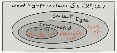
The previous question was answered positively for convex and star-shaped hypersurfaces by Weinstein\citerefCGWeinstein:1978a and Rabinowitz \citerefCGRabinowitz:1978a, respectively. Weinstein isolated key geometric features of a star-shaped hypersurface in and introduced the notion of hypersurface of contact type in a symplectic manifold.
Conjecture 4.1.9 (Weinstein conjecture \citeintroWeinstein:1979a).
A closed hypersurface 777 in general, in any symplectic manifold . of contact type with trivial first real cohomology carries a closed characteristic.
The Weinstein conjecture in was confirmed by Viterbo \citerefCGViterbo:1987a, even without any assumption on the first cohomology. More generally, existence of a Reeb loop for any contact form on the 3-sphere, even for any closed orientable contact 3-manifold with trivial , was shown by Hofer \citerefCGHofer:1993a and generalized to arbitrary by Taubes \citerefCGTaubes:2007a; cf. \citerefCGHutchings:2010a. Let us now follow Weinstein identifying the key geometric features. Consider the radial vector field
| (4.1.4) |
The (local) flow generated by is called Liouville flow.
Exercise 4.1.10.
Show that is a Liouville vector field, i.e. .
Definition 4.1.11.
A closed hypersurface in is called star-shaped (with respect to the origin) if it is transverse to , see Figure 4.2, or equivalently if the projection , , restricts to a diffeomorphism .
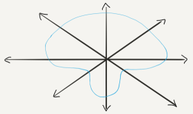
Remark 4.1.12 (Contact type energy surfaces ).
-
(i)
Existence of the Liouville vector field has strong geometric and dynamical consequences: Transversality of along an energy surface induces on some neighborhood the structure of a foliation whose leaves are energy surfaces , i.e. Liouville flow copies of . The apriori slightly obscure condition that is a symplectic dilation, that is , causes that the copies are even dynamical copies in the sense that the linearized diffeomorphisms identify the characteristic foliations and isomorphically; cf. (4.4.8) and Figure 4.4.
-
(ii)
Conclusion: Given an energy surface , the two key structures are, firstly, existence near of a Liouville vector field , that is having the dilation property , which is, secondly, transverse to . Such pair is called an energy surface of contact type.
-
(iii)
Alternative definition: One can show, see Section 4.4, that existence of in (ii) is equivalent to existence of a 1-form on itself such that, firstly, the restriction is (thus is the characteristic line bundle in (4.1.3)), and such that, secondly, the -form is non-vanishing on (evaluation is non-trivial ,888 Thus , hence , so in . see Figure 4.3).
-
(iv)
Given data as in the previous item (iii), the two conditions
uniquely determine a vector field on the contact type energy surface , called the Reeb vector field associated to .
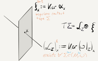
Exercise 4.1.13 (For contact type energy surfaces Hamiltonian and Reeb dynamics coincide up to reparametrization).
Given the data and in the previous item (iv) where for some . Show that for some non-vanishing function on . [Hint: .]
Example 4.1.14 (Non-contact type).
An energy surface diffeomorphic to the sphere, but not of contact type is shown in [HZ11, §4.3 Fig. 4.8].
4.2 Contact manifolds
Exercise 4.1.13 shows that the dynamics on a contact type hypersurface is determined, up to reparametrization, by the -form on itself, independent of the ambient symplectic manifold.
Definition 4.2.1.
A contact form on a ()-dimensional manifold is a 1-form on such that is at any point a non-degenerate skew-symmetric bilinear form on the subspace of the tangent space. The hyperplane distribution is called a contact structure and a contact manifold.
The Gray stability theorem, see e.g. [Gei08, Thm. 2.2.2], tells that for any given smooth family of contact structures there is a smooth family of diffeomorphisms of such that . But there is no such result for contact forms. This indicates that contact forms are objects less geometrical than contact structures.
Exercise 4.2.2 ( contact ).
Given a contact form , show:
-
(a)
At every the co-vector is non-zero, thus the vector space is necessarily of dimension , in other words a hyperplane.
-
(b)
The defining condition of a contact structure , namely being non-degenerate on , is equivalent to being a volume form on , i.e. this -form is at no point of the zero-form.
-
(c)
The kernel is a line bundle over and . There is a unique ’unit’ section of the line bundle determined by and called the Reeb vector field associated to . The (local) flow generated by on is called Reeb flow associated to and denoted by .999 The dynamical behavior of Reeb vector fields associated to two contact forms representing the same contact structure is in general very different.
- (d)
-
(e)
The distribution is co-oriented.
Exercise 4.2.3 (Contact manifolds are orientable).
Suppose is a contact manifold of dimension . Show that induces an orientation of . If is even, then this orientation only depends on the hyperplane distribution , but not on the choice of contact form whose kernel is . [Hint: Pick .]
Exercise 4.2.4 (Reeb flow preserves contact structure).
Show that the Reeb flow preserves the contact form , thus
the contact structure .
[Hint: Check that .]
Exercise 4.2.5 (Standard contact structure on ).
Consider with coordinates and set and . Check that is a contact form on and is spanned by the vector fields and whose commutator is the vector field that is transverse to the plane field .
4.3 Energy surfaces in
Throughout denotes a symplectic manifold of dimension . This section parallels Section 4.1 on energy surfaces in . We don’t repeat proofs.
Define the characteristic line bundle of a closed hypersurface by
Whereas any connected closed hypersurface in is a regular level set of some Hamiltonian , the situation is slightly different in a manifold.
Exercise 4.3.1.
Suppose is a simply-connected manifold. Then any connected closed hypersurface is a regular level set for some function . [Hint: Cf. Lemma. 4.1.2.]
Exercise 4.3.2.
For a closed hypersurface are equivalent:
-
(i)
is orientable.
-
(ii)
is co-orientable.
-
(iii)
is orientable.
-
(iv)
is a regular level set with defined on a neighborhood .
-
(v)
There exists a parametrized family of hypersurfaces modeled on , that is a diffeomorphism
(4.3.5) onto some neighborhood of that has compact closure and such that . We abbreviate and sometimes we denote by .
Remark 4.3.3.
An energy surface in a symplectic manifold is a closed regular level set of the form where is a function and is a regular value. We may assume that is of the form ; otherwise, add a constant to . Note that an energy surface is a closed co-/orientable hypersurface that may consist of finitely many components. As earlier in Section 4.1, a non-vanishing section of is provided by the Hamiltonian vector field of any Hamiltonian having as regular level set. A closed characteristic on an energy surface is an embedded circle , likewise denoted by the letter , such that . Recall from (2.3.22) that denotes the set of closed characteristics on the energy surface .
4.3.1 Stable hypersurfaces
Definition 4.3.4.
A closed hypersurface is called stable if there is a parametrized family modeled on such that for each the linearization
is a bundle isomorphism.
4.4 Contact type hypersurfaces in
In \citeintroWeinstein:1979a Weinstein introduced the following notion; cf. Conjecture 4.1.9.
Definition 4.4.1.
A closed hypersurface in a symplectic manifold is said to be of contact type if is co-orientable111111 Corresponds to in the alternative Definition 4.4.6. Moreover, co-orientability of enables extensions from to neighborhoods; cf. Exercise 4.3.2. and there is a 1-form on such that
-
(i)
, that is the restriction to is exact.
-
(ii)
is non-vanishing on the characteristic line bundle (except zero section)
More precisely, condition (ii) means that evaluation is non-trivial at any point , likewise (cf. Figure 4.3)
Exercise 4.4.2 (Contact type hypersurfaces are contact manifolds).
To see that a contact type hypersurface
in a symplectic manifold
is a contact manifold with contact structure
show the following.
a) The linear functional is non-zero
at any point .
So is a -plane distribution
in the tangent bundle .
b) Show that restricts
to a non-degenerate two-form on , denoted by .
c) Show that is a volume form on
. (Thus such orients .)
[Hint: b) .
c) .
Recall Exercise 4.2.2 (b).]
Remark 4.4.3 (Reeb flow on contact type hypersurface).
The characteristic line bundle of a contact type hypersurface admits by co-orientability a natural section, namely the Reeb vector field normalized by .
There is a second, of course equivalent, definition of contact type which reveals more of the interaction of contact type with the ambient symplectic manifold. The key element is a vector field transverse to – a useful property to generate copies of – and which dilates the symplectic form:
Definition 4.4.4.
A vector field on a symplectic manifold is called a Liouville vector field, or an Euler vector field, if .
Exercise 4.4.5.
If is Liouville on an open subset , then so is for any function .
Definition 4.4.6.
A closed121212 Assuming closed, that is compact and without boundary, makes several things so much simpler: Firstly, transversality is much easier to handle and, secondly, flows on are complete. hypersurface is said to be of contact type if some neighborhood of admits a Liouville vector field transverse to , in symbols . In case of global existence, namely , the hypersurface is said to be of restricted contact type. The Liouville flow is the flow of on . It satisfies wherever it is defined.131313 Thus a closed symplectic manifold cannot admit a global Liouville vector field.
Both definitions of contact type are equivalent
: Given a Liouville vector field on , define
| (4.4.6) |
to obtain the desired 1-form on . Abbreviate and . Then indeed and for any non-zero , together with as , we have that
| (4.4.7) |
: This way is harder as it involves in the first step to extend the 1-form from to a 1-form on some neighborhood of such that ; see [HZ11, §4.3 Le. 3]. Once one has the extension, the identity determines . On one has . To show observe that now in (4.4.7) the right hand side is non-zero, thus cannot be in as already is.
Geometrical and dynamical consequences of contact type
Suppose is a closed hypersurface of contact type. Let and be the two associated structures, one corresponding to the other one (see discussion right above), on some neighborhood of .
The contact type property has powerful geometrical and dynamical consequences illustrated by Figure 4.4:
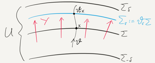
Transversality leads to a foliation of a neighborhood of by copies of under the Liouville flow , that is by the hypersurfaces defined by for small. These copies are even dynamical copies in the sense that the linearization of the diffeomorphism identifies the characteristic foliations and isomorphically.
To see this consider the parametrized family of hypersurfaces modeled on :
| (4.4.8) |
Here is a sufficiently small constant whose existence is guaranteed by compactness of ; choose for the image of . Use in (2.3.20) and to obtain the identity
Given some non-zero vector , then
for every . So the non-zero vector lies in . Thus
| (4.4.9) |
is an isomorphism of line bundles proving that contact type implies stable. Hence induces a bijection , . This motivates Definition 4.3.4.
Exercise 4.4.7 (Stable, but not of contact type).
Show that the hypersurface in the symplectic manifold is stable, but not of contact type. Here is any symplectic form on ; cf. Exercise 2.0.2.
4.4.1 Energy surfaces of contact type
Proposition 4.4.8.
Suppose a closed hypersurface in a symplectic manifold is both, firstly, of contact type with respect to some Liouville vector field on some neighborhood of and, secondly,141414 This assumption is void if is bounding: One easily constructs even globally on . a regular level set of some function . In this case the Reeb vector field and the Hamiltonian vector field are pointwise co-linear along . In symbols, along it holds that
| (4.4.10) |
for some non-vanishing function on . In other words, on the Reeb flow and the Hamiltonian flow coincide up to reparametrization.
Exercise 4.4.9 (Reeb flows on level sets are Hamiltonian near151515 Reeb flows on bounding contact type hypersurfaces are Hamiltonian for some . the level set).
Suppose the regular value of in Proposition 4.4.8 is zero; otherwise replace by . Firstly, extend the non-vanishing function in (4.4.10) from to a non-vanishing function on some open neighborhood, still denoted by and , constant outside a compact neighborhood of . [Hint: Co-orientability of , tubular neighborhoods .] Secondly, show that
-
•
zero is a regular value of the product function ;
-
•
the pre-image is still ;
-
•
along there are the identities .
[Hint: As it helps that is the pre-image of zero.]
4.5 Restricted contact type – exact symplectic
Exercise 4.5.1.
Let be a closed hypersurface
in a symplectic manifold .
a) If is of restricted contact type, see
Definition 4.4.6, with respect to a Liouville vector
field on , then is an exact symplectic
form with primitive .
In particular, the manifold cannot be closed.
b) If is exact, then every
simply-connected closed hypersurface of contact type is of
restricted contact type.
Definition 4.5.2.
An exact symplectic manifold is a manifold with a -form such that is a symplectic form. It automatically comes with the associated Liouville vector field determined by .
Exercise 4.5.3.
Show and the following. An exact symplectic manifold is necessarily non-compact. The boundary of a compact exact symplectic manifold-with-boundary is necessarily non-empy.
Exercise 4.5.4 (Liouville vector fields are outward pointing).
Suppose is a compact exact symplectic manifold-with-boundary and consider the associated Liouville vector field defined by on . Suppose that . (In other words, suppose that the boundary is of (restricted) contact type with respect to .) Let be inclusion and set .
-
(i)
Use the fact that lies in the kernel of , i.e. , to prove the relation
between the natural volume form on and its primitive. Recall that the restriction is a volume form on .
-
(ii)
Let be equipped with the orientation provided by and let the boundary be equipped with the induced orientation according to the ’put outward normal first’ rule; cf. [GP74, Ch. 3 §2]. Verify that
where the first identity is Stoke’s theorem; see [GP74, Ch. 4 §7]. Let be an outward pointing vector field along . Then verify that the integral is a positive multiple of due to the ’put outward normal first’ rule. So points in the same half-space as , that is the outer one. Hence generates a complete backward flow.
4.5.1 Bounding hypersurfaces of restricted contact type
An exact symplectic manifold already comes equipped with the globally defined associated Liouville vector field determined by the identity
Proposition 4.5.5 (Defining Hamiltonians).
Suppose is a bounding hypersurface in an exact symplectic manifold transverse to the associated Liouville vector field on .161616 Such is of (restricted) contact type with . Denote the closure of the inside of by . Then there is a global Hamiltonian with regular level set such that is negative171717 If one does not prescribe the same sign for all ’s inside and the opposite sign outside, then one looses convexity of the space of such, since . inside , equal to a positive constant outside some compact neighborhood of , and such that the Hamiltonian and the Reeb vector field coincide
| (4.5.11) |
Such is called a defining Hamiltonian for the bounding (restricted) contact type hypersurface ; see Figure 5.1. The space of defining Hamiltonians, denoted by , is convex.
Proof.
Use a tubular neighborhood of to define near and then, using that bounds, extend that function, say by , to the remaining parts of the inside/outside of . Then along for some non-vanishing on by (4.4.10). Use again that bounds to extend to a non-vanishing function on . Then the product function has the desired properties since on ; cf. Exercise 4.4.9. Convexity essentially follows from the identity and the chosen regular value being zero. ∎
4.5.2 Convexity
One gets a natural ambience of Rabinowitz-Floer homology by replacing
by
What is the difference? Whereas the restriction to needs to become contact only after adding some exact -form on , non-compactness of exact symplectic manifolds is tamed and made ’controlable’ outside compact parts by requiring what is called the manifold being convex, or cylindrical, near infinity; see \citeintroEliashberg:2000a and \citerefRFBourgeois:2003a. From now on and are connected manifolds.
Definition 4.5.6.
A convex exact symplectic manifold consists of a connected manifold of dimension equipped with a 1-form such that
-
(i)
is a symplectic form on and
-
(ii)
the exact symplectic manifold is convex at infinity, that is there is an exhaustion of by compact manifolds-with-boundary such that is a contact form on for every .
Remark 4.5.7.
Suppose is a convex exact symplectic manifold. Given any compactly supported (smooth) function on , then is also a convex exact symplectic manifold: Indeed the 1-forms and , called equivalent -forms, generate the same symplectic form on . One obtains a suitable exhaustion by forgetting the first ’s, use only those on which .
By Exercise 4.5.4 the associated Liouville vector field points out of along . So the Liouville flow is automatically backward complete. A convex exact symplectic manifold is called complete if the vector field generates a complete flow on . If outside some compact set one says that has bounded topology.181818 To understand this choice of terminology recall that Morse theory describes the change of topology of sublevel sets when crosses a critical level. But critical points of are the zeroes of the gradient vector field , whatever Riemannian metric one picks. Call a subset displaceable if
for some compactly supported Hamiltonian .
Exercise 4.5.8.
a) If is a convex exact symplectic manifold, then so is its stabilization . The 1-form on is given by . b) In every compact subset is displaceable.
Main examples of convex exact symplectic manifolds are
- •
-
•
cotangent bundles equipped with the Liouville form and the canonical fiberwise radial Liouville vector field , see (4.5.12). These are complete and of bounded topology whenever the base manifold is closed. More generally,
-
•
Stein manifolds, see \citerefCGEliashberg:1990a,Eliashberg:1991a or [CE12, Thm. 1.5].
Cylindrical ends
Symplectic manifolds with cylindrical ends have been introduced to construct symplectic field theory (SFT) in \citeintroEliashberg:2000a.
Exercise 4.5.9.
Show that a convex exact symplectic manifold
is complete and of bounded topology iff
there exists an embedding ,
for some closed, not necessarily connected, manifold ,
such that with contact form
and such that
is compact.
[Hint: Apply the Liouville flow to for some large ;
cf. Figure 4.5.]
Each connected component of is called a cylindrical end of and comes equipped with the symplectic form .
Definition 4.5.10.
A -compatible almost complex structure on , i.e. , is called cylindrical if it is cylindrical on the cylindrical ends: Namely, the corresponding almost complex structure on
-
•
couples Liouville and Reeb vector field, that is along ;
-
•
leaves invariant;
-
•
is invariant under the semi-flow for .
Concerning existence of cylindrical almost complex structures see \citerefRF[§2 §3]Bourgeois:2003a or [Abb14, §2.1].
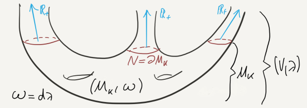
Convex exact hypersurfaces
Definition 4.5.11.
A convex exact hypersurface in a convex exact symplectic manifold is a connected closed hypersurface such that
-
(i)
there is a contact 1-form on such that is exact and
-
(ii)
the hypersurface is bounding,191919 Assuming that bounds, in particular being connected and closed, together with being of codimension in a symplectic manifold, is a sufficient condition that admits a defining Hamiltonian – thereby relating Reeb and Hamiltonian dynamics. say . (So has two connected components, one of compact closure, namely , the other one not.)
Remark 4.5.12.
The next Exercise 4.5.13 shows that a convex exact hypersurface in a convex exact symplectic manifold and with associated contact form is of restricted contact type with respect to an equivalent -form which restricts to the same contact form . Moreover, the new Liouville vector field, given by where , is still transverse to and still outward pointing; see Exercise 4.5.4.
Exercise 4.5.13.
Consider a convex exact hypersurface in with associated contact form . Show the following.
-
(a)
There is a compactly supported function such that the -form on restricts to .
-
(b)
The new Liouville vector field is given by and it is transverse to whenever is.
[Hint: (a) Consult \citeintro[p. 253 Rmk. (2)]Cieliebak:2009a if you get stuck.]
For a list of further useful consequences see \citeintro[p. 253]Cieliebak:2009a. For instance, a closed hypersurface is bounding whenever . This holds, for example, if is Stein of dimension or a stabilization.
4.5.3 Cotangent bundles
Given a closed manifold of dimension , consider the cotangent bundle with its canonical exact symplectic form.
Exercise 4.5.14.
Show that determined by takes in natural local coordinates the form of a fiberwise radial vector field, namely
| (4.5.12) |
It is called the canonical or fiberwise radial Liouville vector field. The fiberwise radial vector field is given by the derivative
| (4.5.13) |
of the curve in the manifold at time . Note that exists on any co/tangent bundle; cf. wiki/Tangent_bundle.
Definition 4.5.15.
A hypersurface is called fiberwise star-shaped (with respect to the zero section) if is bounding, disjoint from the zero section, and transverse to the fiberwise radial vector field.202020 Why is fiberwise radial fine, whereas in one uses the fully radial vector field (4.1.4)?
Exercise 4.5.16.
The intersection of a fiberwise star-shaped hypersurface with each fiber is diffeomorphic to a sphere of dimension .
Exercise 4.5.17.
Pick a Riemannian metric and a smooth function on , consider the Hamiltonian . Show that if , then is a fiberwise star-shaped hypersurface; cf. [HZ11, (4.11)].
Example 4.5.18 (Canonical contact structure on ).
The unit sphere cotangent bundle of is fiberwise star-shaped and of restricted contact type in . In other words, the boundary of the unit disk cotangent bundle of the closed Riemannian manifold is fiberwise star-shaped and of restricted contact type.
4.6 Techniques to find periodic orbits
For convenience of the reader we enlist and summarize, following [HZ11], some key techniques to find closed flow lines of (autonomous) Hamiltonian systems.
4.6.1 Via finite capacity neighborhoods
Based on the Hofer-Zehnder capacity function established in [HZ11, Ch. 3] one derives the following existence results for closed Hamiltonian flow lines.
-
•
Nearby existence [HZ11, Thm. 4.1, p.106]. Given a closed regular level set that admits a (bounded) neighborhood of finite capacity , then the set of closed characteristics is non-empty for some sequence . (There is even a dense subset of of such ’s.)
Idea of proof: Use freedom in choosing the Hamiltonian representing to pick a certain ’radial’ one .
-
•
Existence on itself. In case the periods of the canonically parametrized212121 For each the solution to with traces out and comes back to itself for the first time at some positive time, say . closed characteristics on are bounded, then itself admits a periodic orbit, too.
Idea of proof: Apply the Arzelà-Ascoli Theorem 3.2.10.
-
•
One-parameter families [HZ11, Prop. 4.2, p.110]. Consider a Hamiltonian loop , said of energy , of period which admits precisely two Floquet multipliers222222 the eigenvalues of the linear map equal to . Application of the Poincaré continuation method shows that belongs to a unique smooth family of periodic orbits parametrized by their energy and whose periods converge to , as .
Idea of proof: Construct a Poincaré section map for , investigate how the eigenvalues of its linearization along are related to the Floquet multipliers of , apply the implicit function theorem.
4.6.2 Via characteristic line bundles
Consider the characteristic line bundle , see (4.1.3), over a closed co-orientable hypersurface in a symplectic manifold . Such is an energy surface of some Hamiltonian defined near ; see Exercise 4.3.2. While the set of closed characteristics is empty in certain situations, e.g. for the Zehnder tori \citerefCGZehnder:1987b, cf. [HZ11, §4.5], for large classes of closed co-orientable hypersurfaces existence of closed characteristics is guaranteed.
They key concept is that of a parametrized family of hypersurfaces modeled on a closed hypersurface , introduced earlier in (4.3.5).
Nearby existence listed above fits into this framework whenever is of finite capacity (construct the diffeomorphism using the normalized gradient flow of , say with respect to an -compatible Riemannian metric on ).
Two classes of hypersurfaces which do admit periodic orbits are the following.
-
•
Bounding hypersurfaces. Suppose bounds a compact submanifold-with-boundary and is a parametrized family modeled on . Then each is the boundary of the symplectic manifold-with-boundary . Now the key property is monotonicity232323 By Lebesgue’s last theorem monotonicity of a function implies differentiability, thus Lipschitz continuity, almost everywhere in the sense of measure theory; for a proof see e.g. [Pug02]. of the function which holds by the (monotonicity) axiom of the Hofer-Zehnder capacity . For details see [HZ11, Thm. 4.3, p.116].
-
•
Stable hypersurfaces. A closed hypersurface is called a stable hypersurface if it admits a rather nice parametrized family modeled on , namely one for which each linearization restricts to a line bundle isomorphism .
Advantage. It suffices to detect a closed characteristic on some member of the family in order to obtain a closed characteristic of the original dynamical system itself. For instance, if in the nearby existence result mentioned above was stable, e.g. of contact type, then . Since a closed hypersurface in admits a bounded neighborhood of finite242424 To see that , pick a ball around and apply the axioms (monotonicity) and (non-triviality) of a symplectic capacity in [HZ11, §1.2]. capacity, this confirms the Weinstein conjecture for contact type hypersurfaces in ; cf. Figure 4.1.
As we saw earlier in (4.4.9), a hypersurface of contact type is stable with respect to the parametrized family produced by the Liouville flow . The linearized flow is a bundle isomorphism between the characteristic line bundles of and .
For an example of a stable hypersurface which is not of contact type see [HZ11, p.122].
alpha
Chapter 5 Fixed energy – Rabinowitz-Floer homology
In 2007 Cieliebak and Frauenfelder considered a version of the action functional that involves an additional real variable (detecting periodic solutions of whatever period), namely the Rabinowitz action functional111 For an exposition of the classical free period action functional see \citerefRFAbbondandolo:2013c.
associated to autonomous Hamiltonians on certain exact222 Exactness of a symplectic manifold implies non-compactness, an inconvenient property which one gets under control by imposing additional conditions, for instance convexity. symplectic connected manifolds . While is the set of -periodic loops, the extra parameter , together with time independence of , causes that a critical point of corresponds to
-
•
either a -periodic Hamiltonian loop that lies on the level set ;
-
•
or a constant (period ) loop sitting at a point ;
see (5.1.3). Negative periods tell that the Hamiltonian loop follows .
Now one can exploit this fixed energy property to study dynamical properties of connected closed hypersurfaces in which can be represented as regular level-zero sets of autonomous Hamiltonians on with compactly supported differentials , called defining Hamiltonians for . A sufficient condition that is of the form is that bounds a compact manifold-with-boundary . However, not all connected bounding energy surfaces admit closed orbits, as we saw in (4.1.2). The tool to prove existence of periodic solutions is a version of Floer homology for the Rabinowitz functional on the extended domain . Recall from Chapter 3 that the analytic key to set up Floer homology is compactness, up to broken flow lines, of the spaces of connecting flow lines. The extra parameter causes non-compactness in certain cases – giving way to non-existence (4.1.2). A sufficient condition to fix this is to require the bounding hypersurface to be of restricted contact type, i.e. with contact form . Consequently by (4.5.11) there is a convex set of defining Hamiltonians whose Hamiltonian vector field is simply equal, along , to one and the same Reeb vector field – but is compact. The identity is furthermore extremely beneficial in the sense that it allows to utilize the analysis carried out in the Hamiltonian setting of Chapter 3. In fact, one can allow slightly more general hypersurfaces; cf. Definitions 4.5.6 and 4.5.11 and Remark 4.5.12.
Assumption 5.0.1.
In Chapter 5, unless mentioned otherwise, we assume that
-
•
is a convex exact symplectic manifold of bounded topology whose associated Liouville vector field generates a complete flow on ;333 By \citeintro[Le. 1.4]Cieliebak:2009a bounded topology and complete flow can be achieved for any convex exact symplectic manifold by modifications outside of .
-
•
is a convex exact hypersurface. Let denote the contact form on and the compact manifold-with-boundary bounded by .
According to our conventions both and are connected. By Exercise 4.5.4 the Liouville vector field is outward pointing along the boundary of . By Remark 4.5.12 we may assume whenever convenient that is the restriction of the primitive of the symplectic form .444 Otherwise, replace by where inherits the properties of .
Differences to Chapter 3. Now the closed orbits cannot lie anywhere in the symplectic manifold , they are constrained to a fixed (regular) energy surface required to be a contact manifold with respect to the restriction ; after changing the primitive of , if necessary. (Equivalently the Liouville vector field determined by is transverse to .) In exchange, now the periods are free – no restriction to period any more. Furthermore, whatever defining Hamiltonian one picks, the Hamiltonian loops are precisely the Reeb loops of the contact manifold and their images are called closed characteristics. So what one is really counting are geometric objects associated to the contact manifold and, as , the way it sits in the exact symplectic manifold . Last, not least, as defining Hamiltonians are autonomous, non-constant periodic solutions come at least in -families. So the functional is at best Morse-Bott, as opposed to Morse.
Under Assumption 5.0.1, appropriately taking account of the, at best, Morse-Bott nature of the functional , Cieliebak and Frauenfelder proved
Theorem 5.0.2 (Existence and continuation, \citeintroCieliebak:2009a).
Under Assumption 5.0.1 Floer homology for the Rabinowitz action functional and with coefficients
is defined. If is a smooth family of defining Hamiltonians of convex exact hypersurfaces , then and are canonically isomorphic.
In particular, as the space of defining Hamiltonians is convex, see (4.5.11), Floer homology does not depend on the defining Hamiltonian, but on the pair , at most. In fact, in \citerefRF[Prop. 3.1]Cieliebak:2010b it is shown independence on the unbounded component of , that is only and its inside, the compact manifold-with-boundary , are relevant for . This justifies the following notation where just serves to abbreviate .
Definition 5.0.3.
The Rabinowitz-Floer homology of a convex exact hypersurface bounding , see Assumption 5.0.1, is the vector space555 To define with integer coefficients is an open problem.
| (5.0.1) |
where is a defining Hamiltonian for .
By Theorem 5.0.2 Rabinowitz-Floer homology does not change under homotopies of convex exact hypersurfaces. An integer grading of exists, see (5.3.30), whenever is simply connected and vanishes over . The following deep result has major consequences, e.g. it reconfirms the Weinstein conjecture for displaceable ; see \citeintro[Cor. 1.5]Cieliebak:2009a and Section 5.4.2.
Theorem 5.0.4 (Vanishing theorem, \citeintroCieliebak:2009a).
If is displaceable, then Rabinowitz-Floer homology vanishes.
The idea of proof is to decompose life into two parts and , identifying and . Then push the Hamiltonian flow of into the first part of life using a young (support in ) cutoff function and, in the second part of life, allow for elderly (support in ) but time-experienced Hamiltonian perturbations . This way one gets to the perturbed Rabinowitz action in (5.4.33) and proving Theorem 5.0.4 reduces to a smart homotopy argument; cf. (5.4.41).
Albers and Frauenfelder \citerefRFAlbers:2010b realized that the critical points of are Moser’s \citerefRFMoser:1978a leaf-wise intersection points (s). They obtained existence results for s by associating (Rabinowitz) Floer homology groups to the perturbed action; see Section 5.4.3.
Outline. In Sections 5.1–5.3 we indicate the proof of Theorem 5.0.2 following closely the original, excellently written, paper \citeintroCieliebak:2009a. We also recommend the survey \citerefRFAlbers:2012a. Section 5.4.3 is on the perturbed action functional and s. In Section 5.5 very briefly we state the relation to loop spaces.
Notation 5.0.5.
Cf. Notation 4.0.1 and Notation 1.0.5. The elements of , in particular, the critical points of , are denoted by . The critical points correspond, firstly, to the points of via constant loops whenever and, secondly, to -periodic Reeb loops ; see (5.1.4).666 Reeb loops are non-constant, as the Reeb vector field is nowhere zero by . The notation is meant to indicate that for negative the loop , equivalently , follows . Connecting trajectories are pairs “upsilon” where and .
5.1 Rabinowitz action – free period
Throughout let
be a convex exact hypersurface in a convex exact symplectic
manifold with symplectic structure ;
see Assumption 5.0.1.
Recall from Section 4.5 that bounds a
compact manifold-with-boundary and comes with the contact form
, whereas
globally carries the Liouville vector field
that is determined by the identity .
Let us repeat from Proposition 4.5.5
the notion of defining Hamiltonian for .
Definition 5.1.1.
A defining Hamiltonian for is an autonomous Hamiltonian , negative on the inside of the hypersurface , zero on , positive outside , constant outside some compact set, and with along (the Hamiltonian vector field extends the Reeb vector field); see (4.5.11) and Figure 5.1. Let be the space of Hamiltonians defining .
The space of defining Hamiltonians is non-empty and convex by Proposition 4.5.5.
Remark 5.1.2.
As the Reeb vector field nowhere vanishes, zero is automatically a regular value of . Furthermore, the manifold and the compact manifold-with-boundary bounded by are canonically oriented by the volume form . Moreover, the orientation of
as boundary of by the put-outward-normal-first convention coincides with the orientation provided by the volume form on ; see Exercise 4.5.4 which also shows that the Liouville vector field points outward along . The gradient of with respect to any Riemannian metric points also outward.
Definition 5.1.3.
For a defining Hamiltonian the (unperturbed) Rabinowitz action functional is defined by
| (5.1.2) |
where is the space of -periodic loops in .
Bringing in the real numbers causes that critical points of not only correspond to integral loops of , as was the case in (3.2.11), but constrains777 To find critical points of a function , say on for illustration, whose domain is cut out by a constraint, say , one introduces a dummy variable called Lagrange multiplier and determines the critical points of the function ; cf. Wikipedia. In our case plays the role of the Lagrange multiplier and is zero. them to lie on energy level zero and allows for periods other than .
Exercise 5.1.4 (Critical points correspond to Reeb loops and points of ).
Show that the critical points of are the solutions and of the ODE and the constraint given by
or, equivalently, of
| (5.1.3) |
[Hint: Show . But where preserves .]
Thus a critical point of corresponds either, in case , to a -periodic 888 Here is just a period, not necessarily the prime period of the Reeb loop . Reeb loop on the contact manifold , or in case to one that runs backwards following , or in case to a constant loop sitting at any point of .999 The appearance of all point loops in addition to Reeb loops – at first glance seemingly an annoying irregularity – is actually the power plant of the whole theory; cf. Remark 5.3.7 (ii). A critical point of the form is called a constant critical point. By (5.1.3) the critical points of do not depend on the defining Hamiltonian. In the notation (2.3.12) there is a bijection
| (5.1.4) |
onto the set given by (and then identified with a set of pairs)
| (5.1.5) |
Here is the set of signed Reeb loops: These are the forward or backward101010 Allowing also for periodic solutions of simplifies things, e.g. the above map (5.1.4) is simply a “bijection” instead of a “ map on non-constant critical points”. periodic Reeb orbits on . To see that the map given by is a bijection define and recall from (2.3.12) that is given by restricted to , subject to direction reversal if , and that .
Definition 5.1.5 (Simple critical points and their covers).
Pick a non-constant critical point of and consider the (embedded) image circle . Suppose , otherwise take . Observe that where is the prime period; see (2.3.10). Thus for some integer . Rescale and by
| (5.1.6) |
The prime period of is and
As is a simple loop, we call a simple critical point of .111111 Let us call the corresponding backward simple critical point. The other ones with image are obtained by subjecting to time shifts leading to an -family denoted by or . As divides the speed factor of , we call it the prime speed of the critical points with image .
The -fold covers of a simple critical point defined by
| (5.1.7) |
are critical points of as well and, up to the -action by time shift, there are no other critical points whose image is . Observe that is constant.
Exercise 5.1.6.
Check the assertions in Definition 5.1.5.
Show
that
, modulo time shift also , is independent of
as long as .
[Hints: Let also be a critical point
with and . Check that both paths
and are Reeb solutions
and their prime periods are and ,
respectively. Hence .
But now the paths and
satisfy the same ODE ,
so they are equal up to time shift.]
Exercise 5.1.7 (Simple Reeb loop associated to via time of first return).
Show the assertions of Exercise 5.1.6 as follows. Pick with and set . Now set and apply the Reeb flow to get the Reeb path for whose image is . (Hence the images of non-constant critical points are closed characteristics.) Let be the time of first return. Check that it does not depend on the initial point in , thereby justifying the notation , as opposed to . Since is a one-parameter group is a period of and as it is the smallest positive one is the prime period of . Thus to belongs the simple Reeb loop
| (5.1.8) |
a diffeomorphism onto its image .
-
a)
Show that for some integer .
-
b)
Show that is the prime speed, hence .
[Hints: a) Show that and observe that . b) The pair is a critical point and is an embedding with image . Hence for some and is, in particular, of period . But , equivalently , implies .]
Exercise 5.1.8 (Action spectrum).
Show that the action value
| (5.1.9) |
of the -fold cover, , of a simple critical point is given by times the prime speed . So by Exercise 5.1.7 the action spectrum , i.e. the set of critical values of , consists of all integer multiples of the prime periods of the Reeb loops, in symbols . The set of periods of the simple Reeb loops is the prime period spectrum of the contact manifold .
Remark 5.1.9 (Critical towers).
By (5.1.7) any simple critical point of , that is a pair of the form , gives rise to a whole critical point tower . The circle acts on the -fold cover of by time shifts
Thus point towers come, at least, as critical circle towers where
So the action functional can be Morse-Bott, at best, but not Morse. The set of simple critical points corresponds to the set of closed characteristics with distinguished point : a) Associate to the embedded circle with distinguished point . Indeed is a closed Reeb orbit, thus a closed characteristic, by Exercise 5.1.7. b) Vice versa, given and , consider the Reeb path . Its prime period is denoted by . Then is a simple critical point of which gets mapped back to and by a). That the map in a) followed by the one in b) is the identity as well holds by Exercise 5.1.7 b). In general, the simple critical points can appear in families larger than circles, unless one has
5.1.1 Transverse non-degeneracy
Recall that a function is called a Morse-Bott function if, firstly, its critical set is a submanifold (whose components might be of different dimensions) and, secondly, the tangent space at every point of is precisely the kernel of the Hessian of at . In view of invariance of the functional under the time shift circle action, non-degeneracy is achievable at most in directions transverse to the circles in generated by the -action.
Theorem 5.1.10 (Transverse non-degeneracy, \citeintroCieliebak:2009a).
There is a residual 121212 cf. Section 3.2.4 subset of the complete metric space of smooth functions on with compactly supported differential such that the following is true. For every the Rabinowitz action functional is Morse-Bott and its critical set consists of together with a disjoint union of (embedded) circles.
Proof.
See \citeintro[Thm. B.1, p.298]Cieliebak:2009a. The proof uses the machinery of Thom-Smale transversality, see Section 3.3.4, with the additional difficulty that the universal section cannot be surjective due to the unavoidable critical circles arising by time shifting non-constant critical points. ∎
Definition 5.1.11.
A contact type hypersurface is called non-degenerate if all Reeb loops are transverse non-degenerate in the sense that the linearized Reeb flow at , where and is the prime period of , cf. Exercise 4.2.4, does not have as eigenvalue.
From now on suppose Assumption 5.0.1. Hence the bounding hypersurface is of restricted contact type. Fix a defining Hamiltonian .
Exercise 5.1.12.
Check that iff is non-degenerate.
[Hint: Cf. Exercise 3.2.13.]
Exercise 5.1.13.
a) Show that there is a convex closed neighborhood of in
such that the zero set of any
element is a convex exact hypersurface of .
(In fact, it is of restricted contact type, if is.)
b) Check that is residual in .
[Hint: a) Given the by globally determined
Liouville vector field , the contact type property of
is equivalent to transversality . But transversality
survives, where ,
whenever is sufficiently close to in . Define
; see (4.4.6).]
Remark 5.1.14.
Given regular Hamiltonians near the defining Hamiltonian of , by Exercise 5.1.13 a) convex combination provides a family
| (5.1.10) |
of bounding restricted contact type hypersurfaces of . While the endpoints of the family are non-degenerate, there is no reason that all members be.
Remark 5.1.15 ( consists of circle towers and ).
If is non-degenerate, i.e. , then consists of finitely many closed characteristics since is compact. The embedded circles correspond, up to fixing a point , likewise modulo time shifts, to simple Reeb loops
see (5.1.8), so by Exercise 5.1.7 b) to simple critical points
| (5.1.11) |
Observe that is the prime period (time of first return) of the Reeb loop and simultaneously the prime speed of the simple critical point . Time shifting and moves the initial point around the circle . Let be the -fold cover (5.1.7) of . Let , so
| (5.1.12) |
are the corresponding circles in arising by time shift; cf. Remark 5.1.9. The components of the critical set are the circles along which the action is constantly and the component of constant loops in where the action is zero; cf. (5.3.18). Note that each critical component is compact and that by non-degeneracy only finitely many of them lie on action levels inside any given compact interval . This is illustrated by Figure 5.2.
5.2 Upward gradient flow – downward count
Pick a defining Hamiltonian . So is constant, i.e. , outside a compact subset of . In order to turn the differential of the Rabinowitz action functional into a gradient, we need to choose a metric on . The fact that is non-compact, as opposed to the symplectic manifold in Section 3.4.1 on fixed-period Floer homology, causes serious difficulties when it comes to prove compactness of moduli spaces of connecting trajectories , due to the lack of an apriori bound; cf. Theorem 5.3.6. The key idea to obtain nevertheless uniform bounds for connecting trajectories is to choose a family of -compatible almost complex structures which are cylindrical, see Definition 4.5.10, along the cylindrical ends of .
Remark 5.2.1 ( on cylindrical ends – causes uniform bound for ’s).
Recall from Exercise 4.5.9 that is chosen as boundary of one of the members of the exhaustion of . Choose larger, if necessary, such that contains . This guarantees that vanishes on the cylindrical ends.
For an metric on is defined by
| (5.2.13) |
Exercise 5.2.2.
The gradient of with respect to the metric is given by
| (5.2.14) |
So for the norm-square of the gradient one gets
| (5.2.15) |
where131313 Here for smooth vector fields along the loop . we used that is compatible with and where
The upward gradient trajectories of are the solutions denoted by the letter “upsilon”
of the elliptic PDE given by
| (5.2.16) |
or, equivalently, the zeroes of a section, cf. (3.3.33), namely
| (5.2.17) |
Remark 5.2.3 (Homology – upward vs. downward gradient flow).
The advantage of using the upward gradient equation is that on cylindrical ends, where , component one of (5.2.17) becomes the well known -holomorphic curve equation141414 The downward gradient leads to the anti -holomorphic curve equation . in which case to obtain an apriori bound for one can simply refer to the literature; see \citeintro[p.268, pf. of Thm. 3.1]Cieliebak:2009a. In order to define nevertheless homology, as opposed to cohomology, one must ensure that the action decreases along the boundary operator . This leads to the non-standard order in the coefficients of in (5.3.23) below. In other words, to define an action decreasing boundary operator , one can either
-
(standard)
count downward flow lines emanating from at time or
-
(present)
count upward flow lines that end at at time .
Figure 5.3 illustrates151515 Be aware that will not count connecting flow lines of , but connecting cascade flow lines ; cf. Figure 5.4. The cascades are unparametrized curves , the are (semi-)finite time, thus parametrized, Morse gradient trajectories along components of the Morse-Bott manifold . the downward count of upward flows.
5.3 Rabinowitz-Floer chain complex
Consider a convex exact hypersurface , say of restricted contact type, in a convex exact symplectic manifold, as in Assumption 5.0.1. Fix a family of almost complex structures compatible with the symplectic structure on and cylindrical along the cylindrical ends; see Definition 4.5.10. Choose the associated inner product on given by (5.2.13).
There are two goals in Section 5.3. Firstly, to associate to a defining Hamiltonian of Floer homology groups with coefficients. Secondly, to show that these are invariant, up to natural isomorphism, not only under changing the defining Hamiltonian , but also under convex exact homotopies of the hypersurface itself. Cieliebak and Frauenfelder \citeintroCieliebak:2009a defined
called Rabinowitz-Floer homology of the convex exact hypersurface which, by assumption, bounds a compact manifold-with-boundary, say .
To construct Floer homology one usually slightly perturbs relevant quantities in a first step, see Section 3.3.4, in order to get to a Morse situation, so one can use the then discrete critical points themselves as generators of the Floer chain groups. Here this is impossible: Since , being defining for , is necessarily time-independent the Rabinowitz action functional will always be invariant under the -action on given by time shifting the loop component . While is therefore never Morse, it is of the simplest Morse-Bott type for generic, called regular, defining Hamiltonian by Theorem 5.1.10. For the critical set is the union of and critical point towers
| (5.3.18) |
as illustrated by Figure 5.2. The floors are compact connected manifolds, namely the ground floor together with the upper () and lower () circle floors given by (5.1.12). It is convenient to identify the constant critical points of , action zero, with the points of the compact hypersurface itself. Remark 5.1.15 describes how each closed characteristic together with a chosen point corresponds to a simple critical point of with whose prime speed is the prime period of the simple Reeb loop that parametrizes the closed characteristic and is determined by the initial condition ; see also Remark 5.1.15.
Remark 5.3.1 (Critical set).
The restrictions and of the action functional to components are constant by Exercise 5.1.8. So it makes sense to speak of the action value of a critical component. As only runs through a finite set, caused by compactness and transverse non-degeneracy of , there can only be finitely many critical components with actions in a given bounded interval ; see Figure 5.2. In other words, the set of critical points
whose actions lie in an interval form a closed submanifold diffeomorphic to a finite union of embedded circles whenever ; otherwise, there is in addition one connected component diffeomorphic to .
Perturbing amounts to perturbing , of course. However, by Exercise 5.1.13 a), small perturbations will not leave the class of convex exact hypersurfaces and even the restricted contact type property of will be preserved.161616 The contact condition is open; cf. Exercise 4.2.2 (b). So from now on
- •
-
•
with defining Hamiltonian ; cf. Exercise 5.1.13 b).
Given such , the goal is to find suitable auxiliary data that allows to define Floer homology181818 meaning that the chain groups should be generated by some finite, or at least discrete, critical set and the boundary should count isolated flow lines connecting critical points and has the property that different choices lead to naturally isomorphic homology groups. A suitable candidate is
| Frauenfelder’s implementation of Morse-Bott theory by cascades \citerefRFFrauenfelder:2004a |
which, in addition, requires to fix a Morse-Smale pair consisting of
-
•
a Morse function and
-
•
a Riemannian metric on the critical manifold .
While the critical set of is not necessarily finite, its subset
| (5.3.19) |
is finite, as the manifold is closed, see Remark 5.3.1, and as is Morse.
Chain groups
For the Floer chain group is defined as the vector space over that consists of all formal sums
of critical points of such that the -coefficients in such a formal sum satisfy the upward finiteness condition
| (5.3.20) |
In words, given a formal sum , one requires finiteness of the number of non-zero coefficients above any given action value .
Definition 5.3.2.
The Floer chain group is the -vector space generated by upward finite formal sums of critical points of the Morse function on the critical set of the Rabinowitz action functional .
Connecting cascade flow lines – upward flows
Given , on the critical manifold (whose components are circles and one component is given by the closed hypersurface according to Theorem 5.1.10) consider the Morse gradient flow generated by the Morse function and the Riemannian metric on through the ODE for smooth maps . Given two critical points , a connecting upward flow line with cascades is a tuple of the form
where is the number of cascades and such that
The notation is meant to indicate unparametrized flow lines or, equivalently, flow trajectories that only differ by shifting the variable are considered equivalent. See Figure 5.4 for a connecting cascade flow line with cascades. Actually each intermediate Morse trajectory comes with a finite time and is defined on a finite time interval, namely
In contrast, the two ends and are semi-infinite Morse trajectories. In any case, neither of the Morse trajectories is invariant under the time- shift action.
More precisely, the tuple starts with a semi-infinite Morse trajectory backward asymptotic to the given critical point and whose position at time zero, namely , is the backward asymptote of some flow trajectory defined on the whole real line, see (5.2.17), where
| (5.3.21) |
The other, positive, asymptote provides the initial point of a finite time Morse trajectory whose endpoint is a backward asymptote . Continuing this way one reaches the final piece, namely the semi-infinite Morse trajectory that starts at the previous backward asymptote point at time and is itself forward asymptotic to the second given critical point . The unparametrized Morse-Bott flow lines are called cascades.
The moduli space of connecting cascade flow lines
| (5.3.22) |
consists of all cascade flow lines connecting and . The following are non-trivial – even in finite dimension – although well known: See \citerefRF[App. A]Frauenfelder:2004a and \citeintro[App. A]Cieliebak:2009a. Firstly, for generic and these moduli spaces are smooth manifolds. Secondly, it is a consequence of the Compactness Theorem 5.3.6 below that the 0-dimensional part of is compact, so a finite set.
Boundary operator and Floer homology
Pick . Since for generic and the 0-dimensional part of the space of connecting flow lines is compact, hence a finite set, the number of elements modulo two
is well defined. Then the Floer boundary operator
is defined as the linear extension of
| (5.3.23) |
for . This is illustrated by Figure 5.3; cf. also Remark 5.2.3.
Exercise 5.3.3.
The boundary operator property follows by standard gluing and compactness arguments, compare Proposition 3.4.3, once one has the Compactness Theorem 5.3.6 for the 1-dimensional part of moduli space, together with finiteness of the number of critical points of the Morse function in any finite action interval or, equivalently, on the closed manifold . By definition Floer homology of the Rabinowitz action functional is the homology of this chain complex, namely
| (5.3.24) |
We already dropped from the notation since does not depend on that choice, up to canonical isomorphism, as follows by the standard continuation techniques detailed in Section 3.4.3. Via continuation one also shows independence of the regular defining Hamiltonian .
Rabinowitz-Floer homology of a convex exact hypersurface
Remark 5.3.4.
Given as in Assumption 5.0.1, observe the following: There is no regular defining Hamiltonian iff itself is already degenerate; see Exercise 5.1.12. Hence fixing non-regularity of is equivalent to perturbing . In practice pick in the dense subset of the small open neighborhood of in provided by Exercise 5.1.13 b). In particular, the zero set is a non-degenerate convex exact hypersurface nearby . The Floer homology of is then defined by (5.3.24). For any two such choices and there is the standard continuation isomorphism on homology.
Rabinowitz-Floer homology of a convex exact hypersurface with defining Hamiltonian is defined by
| (5.3.25) |
By continuation does not depend on the choice of ; cf. Remark 5.1.14. Observe that lies in and in : It is defining for the non-degenerate convex exact hypersurface nearby . For -equivariant Rabinowitz-Floer homology see \citerefRFFrauenfelder:2016a.
5.3.1 Compactness of moduli spaces
Definition and property of the boundary operator both hinge on compactness properties of the moduli spaces of connecting flow lines with cascades. Recall that a connecting cascade flow line consists of (semi-)finite Morse gradient trajectories191919 in general not connecting ones: Morse trajectories have finite life time, except the initial and ending one which are semi-infinite, also called semi-connecting. along the critical set of and the cascades themselves. Cascades are, modulo -shift, connecting trajectories of between two critical sets in .202020 Connecting trajectories necessarily live on the infinite domain and their moduli spaces are subject to division by the free -action given by shifting the -variable. While compactness up to broken trajectories for Morse trajectories can even be handled within finite dimensional dynamical systems, see e.g. [Web], in the case of cascades compactness of the loop space component is also standard, but this is not so for the Lagrange multiplier component . Let us detail this: To prove compactness up to broken trajectories of the set of trajectories that are subject to a uniform action bound
| (5.3.26) |
for all times , the following apriori bounds are sufficient: Namely,
-
(i)
a uniform bound on ;
-
(ii)
a uniform bound on ;
-
(iii)
a uniform bound on (thus on ).
(i) is fine due to our choice of cylindrical almost complex structures; see Remark 5.2.3. (ii) was new and required new techniques when it was established in \citeintro[§3.1]Cieliebak:2009a. Thus we shall outline their argument below. (iii) follows from the exactness assumption of the symplectic form via standard bubbling-off analysis as shown in Section 3.4.1.
Exercise 5.3.5.
Doesn’t one need a uniform bound on the derivative as well? And why is the bound requirement (iii) for the derivative not listed directly after condition (i) for itself?
Let us state the compactness theorem in a rather general form that will serve simultaneously
-
•
the continuation problem, where -dependent Hamiltonians appear;
-
•
the proof of the Vanishing Theorem 5.0.4, where the rescalings help.
Of course, the following compactness theorem for families requires three bounds as in (i–iii) which are, in addition, uniform in the family parameters.
Theorem 5.3.6 (Cascade compactness).
Suppose that is a smooth function such that each Hamiltonian defines a convex exact hypersurface and is a smooth function such that each integrates to one. Let and be constants as provided by \citeintro[Prop. 3.4]Cieliebak:2009a,212121 \citeintro[Prop. 3.4]Cieliebak:2009a is a generalization of Proposition 5.3.8 to families . and suppose that the following inequality holds
| (5.3.27) |
Then the following is true. Assume that is a sequence of trajectories of the -dependent gradient and there are bounds such that
for all times and that
Then there is a subsequence, still denoted by , and a trajectory of such that the subsequence converges to in the -topology.
Proof.
[Thm. 3.6]Cieliebak:2009a. ∎
Uniform bounds for multiplier paths – contact type enters
For simplicity we only consider the case of trajectories of the -independent gradient . Moreover, we only sketch proofs; for details see \citeintro[§3.1]Cieliebak:2009a.
Remark 5.3.7 (Contact type of enters).
(i) So far the geometric condition on to be not just any bounding hypersurface in , but a convex exact one,222222 We assume contact type for , otherwise, add an exact form to ; cf. Exercise 4.5.13. has not been used. That will change now in order to obtain a uniform bound for the Lagrange multiplier components of all trajectories subject to the same action bounds and as in (5.3.26).
(ii) Some condition on the energy surface is indeed necessary, given that there are energy surface counterexamples in to the Hamiltonian Seifert conjecture; cf. (4.1.2). But even in the absence of closed characteristics the constant loops corresponding to the points of are still critical points of thereby giving rise to nontriviality ; cf. Exercise 5.3.17 and \citeintro[Pf. of Cor. 1.5]Cieliebak:2009a. But this would contradict the Vanishing Theorem 5.0.4 since in any compact subset is displaceable.
Proposition 5.3.8.
Let be a defining Hamiltonian. Then there are constants and such that for pairs it holds
The proposition tells that near critical points the multiplier part of a pair is bounded in terms of the pair action. So if is one element of a whole trajectory subject to the bound (5.3.26), thus
| (5.3.28) |
then the proposition provides a uniform bound on for near . So it remains to deal with along compact intervals in , one compact interval for each trajectory of the, generally non-compact, family under consideration.
Corollary 5.3.9 (Uniform bound).
Let be a trajectory of along which the action remains in a compact interval, say in ; cf. (5.3.26). Then the -norm of is bounded uniformly in terms of a constant that depends on , but not on .
Sketch of proof of Proposition 5.3.8.
(For details see \citeintro[Prop. 3.2]Cieliebak:2009a.) The key input, due to being both an energy surface and of contact type with respect to , is the coupling of Hamiltonian and Reeb dynamics along ; see (4.5.11). To illustrate the effect of the coupling note that for a critical point of
| (5.3.29) |
This actually solves Exercise 5.1.8. Let’s see how much of this identity survives for a general pair whose only restriction is that the loop part must stay in a small neighborhood of .
I. There are constants and with the following significance. For every pair whose loop part remains -near to in the sense that the Lagrange multiplier satisfies the estimate
The key step is to obtain the two constants. By compactness of and zero being a regular value of the closure of is compact for sufficiently small . Now choose smaller, if necessary, such that
Such exists since along : To see this use contact type, see (4.5.11), and the definition of , see Exercise 4.2.2 (c). The constant is finite since is of compact closure. The desired estimate is a rather mild generalization of (5.3.29), see \citeintro[p.264]Cieliebak:2009a.
II. For each there is a constant such that whenever a pair satisfies , then the loop part remains in .
To show II one first analyzes in two cases, in each case
forgetting one of the two components of ;
see (5.2.15). Excluding both cases yields II.
Case 1:
There are times with
and .
In this case by periodicity of and continuity of there are two points,
again denoted by , with and
on .
Set
and forget component two in (5.2.15) to get232323
Use that by Cauchy-Schwarz
for .
The omitted steps, using e.g. ,
are detailed in \citeintro[p.265]Cieliebak:2009a.
Case 2:
The loop lives outside .
Forgetting component one
in (5.2.15)242424
To see the identity note that is non-zero, hence will
not change sign; cf. (5.4.43).
To prove Step II pick any , set
and assume satisfies . Neither case 1 nor 2 applies to . So hits ( case 2), but then it cannot leave ( case 1).
III. We prove the proposition.
Choose the constants and of Steps I and II, respectively, and set . Suppose . Then by Step II the loop part remains in , hence Step I applies and yields
This concludes the outline of the proof of Proposition 5.3.8. ∎
Proof of Corollary 5.3.9 (Trajectories).
Pick as in Proposition 5.3.8.252525 By Step II above given any sufficiently small constant . Set and . The key tool is the quantity given for by
This quantity helps twice. Firstly, given a trajectory and a time element of gradient norm (otherwise ), the function measures for how long the gradient norm will remain , so for how long the trajectory will not get too close to a critical point. By assumption (5.3.26) we get the estimate
which holds true for every and, by the way, also shows finiteness . Secondly, for any the gradient norm of the trajectory element at time is . Hence the pair satisfies the assumption of Proposition 5.3.8, so together with the action bound in (5.3.28) we get that
for every . Putting things together one obtains the desired estimate
for every using that satisfies the gradient flow equation (5.2.17). ∎
5.3.2 Continuation
To prove invariance of Floer homology defined
by (5.3.24) for a
convex exact hypersurface with regular defining Hamiltonian ,
not only under change of the regular defining Hamiltonian, but even under convex
exact deformations of itself, see Theorem 5.0.2,
suppose is a smooth family of defining
Hamiltonians of convex exact hypersurfaces in
.
The construction of natural continuation maps follows precisely
the same steps as in Section 3.4.3,
see \citeintro[§3.2]Cieliebak:2009a for details,262626
The -homotopy of -homotopies
in \citeintro[p. 276]Cieliebak:2009a should be
, not ,
in order that for each the initial point (at )
coincides with the endpoint (at ) of the -homotopy
and so the two homotopies can be
concatenated.
once appropriate compactness properties of the spaces of
connecting cascade flow lines for the -dependent
gradient have been established.
The only problem is that condition (5.3.27)
on smallness of the product
might not be satisfied in general.
A common technique is to carry out the homotopy
in steps, namely sucessively via the homotopies
and show that the continuation map provided by each of them is an isomorphism. Since
condition (5.3.27) is satisfied indeed for each homotopy whenever is chosen sufficiently large. But the composition of the continuation isomorphisms provided by each individual is the continuation map, hence isomorphism, provided by ; cf. (3.4.53).
To show that is well defined by (5.3.25) requires to pick as in Remark 5.3.4 and show that by continuation. For this it is sufficient, as mentioned above, to have a smooth family of defining Hamiltonians of convex exact hypersurfaces in interpolating and . Note that such family is obtained simply by convex combination of and ; see Remark 5.1.14.
In \citerefRF[Prop. 3.1]Cieliebak:2010b it is even shown independence on the unbounded component of , that is only and its inside, the compact manifold-with-boundary , are relevant for . This leads to the notation for , often abbreviated by ; see Definition 5.0.3.
5.3.3 Grading
Suppose is a convex exact hypersurface, say of restricted contact type, and is defining. Throughout Section 5.3.3 suppose that
-
(i)
the contact manifold is simply-connected, that is ;
-
(ii)
is Morse-Bott;
-
(iii)
has trivial first Chern class over , that is ;
-
(iv)
is Morse on the critical manifold .
Under these conditions there exists an integer grading taking values in , see (5.3.30), of the Rabinowitz-Floer complex in terms of the sum of the transverse Robbin-Salamon index of (rescaled) Reeb loops and the signature index of a critical point of the Morse function . For non-degenerate the transverse Robbin-Salamon index reduces to the transverse Conley-Zehnder index and will be half-integer valued.
Transverse Robbin-Salamon index
Pick a critical point of , i.e. satisfies by (5.1.3). In words, the loop integrates the rescaled Reeb vector field .272727 Alternatively consider the corresponding -periodic Reeb path with on the -dependent interval ; see Exercise 5.1.7. Recall that defines a – with respect to symplectic – vector bundle of rank and that . By (i) pick a smooth extension of the loop and choose a unitary trivialization of the symplectic vector bundle . Then the linearization of the flow generated by , informally called the linearized rescaled Reeb flow, provides along the trajectory by (ii) a path in the symplectic linear group with initial point and Robbin-Salamon index denoted by
It is called the transverse Robbin-Salamon index of the critical point or, alternatively, the -periodic solution of the rescaled Reeb vector field .
Exercise 5.3.10.
Show that the definition of is independent of the choice of, firstly, the extending disk by (iii) and, secondly, of the unitary trivialization.
Exercise 5.3.11.
Calculate for constant critical points of .
Transverse Conley-Zehnder index
Suppose a critical point of is transverse non-degenerate;282828 Call transverse non-degenerate iff and the corresponding Reeb loop is. cf. Definition 5.1.11 and Exercise 5.1.12. So the image is an isolated closed characteristic of . Moreover, the corresponding path in ends away from the Maslov cycle, i.e. the path is an element of , so the Robbin-Salamon index is nothing but the Conley-Zehnder index of this path. In order to implicitly signalling the assumption of transverse non-degeneracy, as opposed to just general Morse-Bott, we use the notation
for transverse non-degenerate critical points and call this index the transverse Conley-Zehnder index.
Exercise 5.3.12 (Half-integers).
Show that is half-integer valued.
Signature index and Morse index
Let be a Morse-Bott function on a finite dimensional manifold . Given a critical point of , recall that the Morse index is the number of negative eigenvalues, with multiplicities, of the Hessian of at . The signature index of is defined by
Exercise 5.3.13 (Morse-Bott).
Let be Morse-Bott. Show that292929 Set and for some, hence any, .
for every connected component of the critical manifold .
Exercise 5.3.14 (Morse).
If is a non-degenerate critical point, then
Morse-Bott grading of the Rabinowitz-Floer complex
Definition 5.3.15 (Grading).
For , define
| (5.3.30) |
Exercise 5.3.16 ( non-degenerate half-integers).
For non-degenerate , show that is half-integer valued for every . Is this also true if is a constant critical point?
Given , consider a connecting cascade flow line , an element of the moduli space defined by (5.3.22). For generic and this space is a smooth manifold whose local dimension303030 dimension of the component that contains at is given by
The first step is non-obvious even for the Morse-Bott cascade complex in finite dimensions; see \citeintro[(65)]Cieliebak:2009a. One crucial ingredient to obtain the first step, cf. \citeintro[(64)]Cieliebak:2009a, is the following even less trivial formula. Let be the moduli space of finite energy trajectories of . By Morse-Bott, firstly, the asymptotic limits in (5.3.21) exist, let be their components of , and secondly the linearization of the gradient equation (5.2.17) at a flow trajectory , cf. (3.3.33), is Fredholm between suitable spaces. By \citeintro[Prop. 4.1]Cieliebak:2009a
For further details concerning index computations see \citeintroCieliebak:2009a and \citerefRFMerry:2011b.
5.3.4 Relation to homology of
Exercise 5.3.17.
If carries no Reeb loops that are contractible in , then
is a grading preserving isomorphism where for any defining Hamiltonian ; see (5.0.1). Why should there be a grading without assuming triviality of and ?
5.3.5 Example: Unit cotangent bundle of spheres
Consider the unit cotangent bundle of the unit sphere in euclidean space equipped with the induced Riemannian metric. Observe that is a hypersurface of restricted contact type of the convex exact symplectic manifold ; see Example 4.5.18. In particular, the restriction is a contact form on the hypersurface that bounds the (compact) unit disk cotangent bundle .
Theorem 5.3.18 (Unit cotangent bundle of unit sphere, \citeintroCieliebak:2009a).
For
Idea of proof (Lacunary principle – Floer homology equals chain complex). One exploits the facts that for the round metric on , suitably normalized, all geodesics are periodic with prime period , that the functional is Morse-Bott,313131 Do not confuse with the stronger notion “transverse non-degenerate” in Theorem 5.1.10. and that the critical manifold is given by (the constant loops – we don’t call them geodesics), together with copies of where labels the periods of the periodic geodesics. Now one picks a Morse function on with precisely four critical points of Morse indices and defines to be the Morse function on which coincides with on each component. Then
Now one pits action knowledge (5.1.9) in terms of the prime period and positivity of the action difference of two critical points and sitting on the two ends of a non-constant connecting trajectory against the facts that the boundary operator decreases the grading precisely by and that can be related via the Morse index theorem for geodesics to the particular Morse indices encountered among the critical points of as mentioned above. In the end, for , one gets to the conclusion that there cannot be a connecting trajectory between critical points of -index difference one. For details see \citeintro[p. 293]Cieliebak:2009a.
5.4 Perturbed Rabinowitz action
To prove the Vanishing Theorem 5.0.4 motivates to allow for more general Hamiltonians in the action functional; cf. \citeintro[§3.3]Cieliebak:2009a. Pick a defining, thus autonomous, Hamiltonian and a young cutoff function323232 The support of , notation , is the closure of its non-vanishing locus .
| (5.4.31) |
The assumption is used in (5.4.43). Let us call the Hamiltonian
| (5.4.32) |
a young Hamiltonian, as its flow is active only in the first half of life. Suppose is a possibly non-autonomous -periodic Hamiltonian. The perturbed Rabinowitz action functional on is defined by
| (5.4.33) |
In the notation of (5.2.17) and taking the same choices, such as a cylindrical almost complex structure with induced metric on , the upward gradient trajectories of are the solutions of the PDE
| (5.4.34) |
Compactness in Section 5.3.1, thus the definition of Floer homology in Section 5.3, goes through for with only minor modifications; see \citeintro[§3.1]Cieliebak:2009a.
5.4.1 Proof of Vanishing Theorem
The Vanishing Theorem 5.0.4 asserts triviality of Rabinowitz-Floer homology whenever is displaceable.
Proof of Vanishing Theorem 5.0.4 – v1
The first version of the proof is short and rather illustrative, hence well suited to communicate the main ideas. But – it has the disadvantage that it involves a class of Hamiltonians for which we haven’t introduced Floer homology ; however, this is done in \citerefRFAlbers:2010b. In other words, in proof v1 the required technical work is moved elsewhere, so we are just left with the nice bits.
The idea is to find Hamiltonians such that there are no critical points
| (5.4.35) |
In this case there are no generators of the corresponding Floer complex. Hence
| (5.4.36) |
The isomorphisms are by continuation. Section 5.3 establishes only, but the same construction goes through for replacing , including the construction of the second continuation isomorphism. The first continuation isomorphism and itself are constructed in \citerefRF[§2.3]Albers:2010b; see Section 5.4.3.
In preparation of the proof of (5.4.35) we take the following choices, given a compactly supported Hamiltonian that displaces . By compactness of the map not only displaces from itself, but also a small neighborhood of . Observe that is contained in for any of its defining Hamiltonians , since 0 is a regular value of . Change or modify , if necessary, such that . Hence this support also gets displaced:
| (5.4.37) |
Now pick an elderly cutoff function
| (5.4.38) |
as illustrated by Figure 5.6 and consider the elderly Hamiltonian, defined by
| (5.4.39) |
Elderly means that the flow of is active only in the second half of life.
Exercise 5.4.1.
Show a) for and b) for . [Hint: a) Footnote.333333 b) Note that with .]
The critical points of are the solutions of the equations
| (5.4.40) |
It remains to prove emptyness (5.4.35). By contradiction suppose that is a solution of (5.4.40). There are two cases.
Proof of Vanishing Theorem 5.0.4 – v2
This version of proof gets away with Floer homology as introduced in Section 5.3 and is based on continuation and the following stronger version of the absence (5.4.35) of critical points of the perturbed action associated to the young Hamiltonians in (5.4.32) and the elderly ones in (5.4.39).
Lemma 5.4.2 (No critical points).
Fix a smooth monotone cutoff function with for and for in order to define a homotopy , and its reverse , between the zero Hamiltonian and the Hamiltonian , namely
For each real parameter value consider the homotopy from the zero Hamiltonian back to itself which is defined by the concatenation
of the homotopy followed by its reverse , as illustrated by Figure 5.7.
Now consider the homotopy, in , of homotopies of Hamiltonians and their corresponding action functionals
The homotopies at and have special properties. The one at is constant, given by , and the one at has – as a consequence of the no-critical-points Lemma 5.4.2 – no connecting flow lines:
Lemma 5.4.3 (No finite energy trajectories).
There is a constant depending only on , , and the action values of two fixed critical points such that the following is true. For each real there are no trajectories of the -dependent gradient converging asymptotically to .
Lemma 5.4.4 (Uniform bound).
Pick and assume that is a trajectory of , for some , converging asymptotically to . Then is uniformly bounded by a constant that depends only on , , , and the action values of .
Lemma 5.4.4 implies compactness of the relevant components of the moduli spaces appearing in the definition (3.4.52) of the continuation homomorphisms
But the are all equal, as the defining homotopies of any two are homotopic, cf. Exercise 3.4.17, and , because it is induced by the constant homotopy, cf. Exercise 3.4.15. But since by Lemma 5.4.3 there are just no connecting trajectories of whenever . Thus we conclude
| (5.4.41) |
But this is only possible if the domain is trivial which is what is claimed by the Vanishing Theorem 5.0.4. Full details are given in \citeintro[§3.3]Cieliebak:2009a.
Let us look at the ideas, at least, how to prove the three lemmas. For details see \citeintro[p. 281-284]Cieliebak:2009a.
No critical points. The proof of Lemma 5.4.2 takes three steps and uses compactness of , that displaces and that and are young and elderly, respectively. Furthermore, it is crucial that has two components, see (5.2.14), whose norms can be played out, one against the other one.
Step 1: There is a constant such that if satisfies
| (5.4.42) |
then
In words, for such loops not both, birth and midlife crisis, can happen under -action, at least one of them requires a rest from the defining Hamiltonian . The proof of this uses that is compact and is displaced by only at the end of life where the young is not supported.
Step 2: There are such that if satisfies (5.4.42) for , then
That is stays away from zero during the first part of life of any such loop . The proof exploits that is elderly and uses Step 1.
Step 3: Pick .
To prove that involves two cases in each of which one
simply forgets one of the two gradient components,
cf. (5.2.15).
If ,
we are done: Just forget component two.
Otherwise, if , Step 2 applies. Forget component one to
obtain that
| (5.4.43) |
Here we used that is young and integrates to one. Concerning the second identity use the non-negativity assumption in (5.4.31) together with the fact that by Step 2 the function is non-zero along the interval , in fact, it is either or .
Exercise 5.4.5.
No finite energy trajectories. This is essentially an integrated version of Lemma 5.4.2. In the -independent case the proof is trivial: Any connecting trajectory has finite energy , namely, it is given by the action difference of the asymptotic limits. But a positive lower gradient bound as in Lemma 5.4.2 contradicts finiteness, so such trajectories cannot exist. The -dependent case is rather similar; see \citeintro[p.283, Step 1]Cieliebak:2009a.
Uniform bound. The proof is similar to the one of the uniform bound on in Section 5.3.1, again built on the quantity . That displaces is not used.
5.4.2 Weinstein conjecture
Theorem 5.4.6.
A displaceable convex exact hypersurface in a convex exact symplectic manifold carries a closed Reeb loop that is contractible in .
The theorem was established in \citerefRFSchlenk:2006a for stably displaceable hypersurfaces of contact type. Recall that if a closed contact type hypersurface is simply-connected, then it is of restricted contact type by Exercise 4.5.1.
Exercise 5.4.7.
Consider a connected closed hypersurface .
a) Show that is bounding and displaceable.
b) Show that
if is, in addition, transverse to some
global353535
A locally near defined is sufficient
whenever ;
cf. Exercise 4.5.1 b).
Liouville vector field , then it is convex exact.
5.4.3 Leaf-wise intersections
Before giving the formal definition of “leaf-wise intersection” let us first switch on light by looking at the circular restricted three body problem in celestial mechanics; cf. [AM78, Ch. 10].
Motivation: Satellite perturbed by comet
Following \citerefRFAlbers:2012b
consider an almost massless particle, the satellite ,
moving in the gravitational field of two huge massive bodies
called primaries, say earth and moon .
By assumption the whole system is restricted to a given
fixed plane and each of the primaries
moves along a circle about their common center of mass.
So the configuration space of the system is rather restricted. Now suppose the satellite, so far moving peacefully on its energy surface
in phase space, gets temporarily influenced by a
comet passing by during a time interval, say of length one.
Suppose the previously autonomously via on moving
satellite receives extra kinetic energy by gravitational attraction
as the comet appears in front at time zero and looses energy when
the comet disappears behind at time one. The comet’s
presence is described by a time-dependent Hamiltonian with
Hamiltonian flow . In other words,
at time zero, say at the phase space location ,
the satellite gets lifted off of following
for one unit of time after which it gets dropped back onto
at .
Let , called the
leaf of , be the whole phase space trajectory of
the satellite as it would happen without the comet’s appearance.
One would probably not expect that the satellite will get dropped back
at to its original trajectory . However if it happens,
the unexpected penomenon
is called a leaf-wise intersection, see Figure 5.9, and is called a leaf-wise intersection point (LIP).
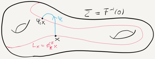
Satellite at deviates under sudden comet influence
,
but happens to end up on its unperturbed trajectory
afterwards
Surprisingly, the phenomenon indeed happens: In certain hypersurfaces of exact symplectic manifolds, for instance such of non-zero Rabinowitz-Floer homology, for any comet there is by \citerefRF[Thm. C]Albers:2010b a satellite position which ends up on its own unperturbed trajectory afterwards. In certain cotangent bundle situations there are, for generic comets, even infinitely many undestroyable satellite trajectories by \citerefRFAlbers:2010c; see also \citerefRF[Thm. 1]Albers:2012b and §2.2 in the survey \citerefRFAlbers:2012a.
Rabinowitz-Floer homology for perturbed action
Let and satisfy Assumption 5.0.1 where is defining. Consider the Rabinowitz action functional in (5.4.33) for possibly non-autonomous elderly Hamiltonians
also called elderly perturbations of . The perturbed functional has a number of useful properties: As time-dependence is allowed for , the functional is Morse for generic , as shown in \citerefRF[Thm. 2.13]Albers:2010b. Thus no Morse-Bott complex will be needed at all. The critical points of correspond to leaf-wise intersections.363636 The map , , is injective, unless for some .
Proposition 5.4.8 (Critical points and LIPs, \citerefRFAlbers:2010b).
If , then lies in and lies on the Reeb leaf .
The definition of Floer homology proceeds pretty much as in Chapter 3 with the little extra twist of an upward finiteness condition, completely analogous to (5.3.20), that takes care of infinitely many critical points. More precisely, given a defining Hamiltonian , pick a young cutoff function as in (5.4.31) and a generic elderly perturbation such that is Morse. Let be the vector space that consists of all formal sums
such that, given , for each there is only a finite number of non-zero -coefficients that belong to critical points of action ; cf. (5.3.20). Let be the space of connecting (upward) gradient trajectories, that is solutions of the PDE (5.4.34), with asymptotic boundary conditions sitting at ; cf. Figure 5.3. For generic -families of cylindrical almost complex structures the space is a smooth finite dimensional manifold that carries a free -action by -shift. Let
be the number (mod 2) of zero-dimensional components of the moduli space of connecting flow lines; cf. (3.4.46). Define the Floer boundary operator on the chain groups analogous to (5.3.23) by linear extension of
By definition Floer homology of the perturbed Rabinowitz action functional is the homology of this chain complex, namely
Theorem 5.4.9 (Invariance of under elderly perturbations, \citerefRFAlbers:2010b).
If is Morse for an elderly perturbation , then
The theorem actually concludes the proof of version one of the Vanishing Theorem 5.0.4; cf. (5.4.36).
Remark 5.4.10 (Rabinowitz Floer for Reeb chords and Voyager missions).
Coming back to the previous space travel motivation, there is practical interest in so-called consecutive collision orbits – of course, in small perturbations of them. In \citerefRFFrauenfelder:2017a consecutive collision orbits, interpreted as Reeb chords, are encoded as critical points of an adequate version of the Rabinowitz action functional. Calculation of the corresponding Rabinowitz Floer homology then leads to infinitely many collision orbits.
The general picture: Coisotropic intersections
The previous situation of a closed codimension one submanifold being foliated by flow lines, that is -dimensional leaves , is the rather special case of the general leaf-wise intersection problem described in the masterpiece \citerefRFMoser:1978a. It is amazing to see how important results fall off as special cases for particular values of the codimension of a closed coisotropic submanifold of a simply-connected exact symplectic manifold of dimension ; see the presentation in \citerefRFMoser:1978a of consequences 1.–4. of the main theorem that asserts existence of leaf-wise intersections.
A codimension submanifold of a symplectic manifold of dimension is called a coisotropic submanifold if every tangent space of is a coisotropic subspace of the corresponding tangent space of . This implies . The collection of symplectic complements turns out to provide an integrable distribution of rank in the tangent bundle . Thus by Frobenius the dimensional manifold is foliated by leaves of dimension .
For the main theorem in \citerefRFMoser:1978a proves existence of at least two fixed points of a symplectic diffeomorphism of a closed simply-connected symplectic manifold, see Remark 1.0.4; the assumption of being simply-connected was removed in \citerefRFBanyaga:1980a.
For one gets to the previously described situation of integral curves of the characteristic line bundle of an energy surface, hence to Reeb dynamics if is of contact type.
For one recovers the Lagrangian intersection problem.
5.5 Symplectic homology and loop spaces
Running out of time and pages, let us just briefly mention that, given a closed Riemannian manifold , Rabinowitz-Floer homology of the unit sphere cotangent bundle , bounding the unit disk cotangent bundle , in the cotangent bundle encodes both homology and cohomology of the free loop space.373737 Recall that in the present text we work with coefficients; for field coefficients see the convention prior to Thm. 1.10 in \citerefRFCieliebak:2010b. It was shown in \citerefRF[Thm. 1.10]Cieliebak:2010b that
| (5.5.44) |
and that for there are isomorphisms involving the Euler class of the vector bundle . Now the grading of is different from the half-integer grading defined earlier in (5.3.30), namely
The isomorphism is obtained by relating via a long exact sequence Rabinowitz-Floer homology to symplectic homology and cohomology of , aka Floer co/homology of the cotangent bundle, and then use the isomorphism (3.5.61). A proof of (5.5.44) by a direct construction is given in \citerefRFAbbondandolo:2009a and a generalization to twisted cotangent bundles in \citerefRFMerry:2011a; see \citerefRFBae:2011a for an alternative method.
alpha
Part III Appendices
Appendix A Function spaces
A.1 Some Banach spaces and manifolds
We shall provide the Banach manifolds and , each admitting a countable atlas modeled on a separable Banach space, that are used in Example 3.3.32.
The separable Banach space for closed
Proposition A.1.1 (The separable Banach space ).
Fix . For a closed manifold the vector space of times continuously differentiable functions equipped with the sum of the sup norms of a function and its derivatives up to order is complete and separable. This remains valid for vector valued functions, that is for .
Idea of proof.
Case .
Asking any topological space, say , just to be compact and Hausdorff
already implies that is complete under the sup norm;
cf. [RS80, Thm. IV.8].
Separability:111
In case of a bounded open subset separability
of follows from density of the (countable) space
of polynomials with rational coefficients;
see e.g. [AF03, Cor. 1.32].
A manifold is metrizable; either exploit second
countable or use a Whitney embedding into some .
So pick a dense sequence in
and for define the function
if
and otherwise. Then the (countable) collection
given by the together with a constant function generates a
countable algebra by taking linear combinations
with rational coefficients of finite products of members of the collection.
The algebra separates the points of ,
thus the closure of in is itself
by the Stone-Weierstrass Theorem; cf. [RS80, Thm. IV.9].
Case . Reduction to :
Consider the isometric linear injection
that maps to the vector whose
components are and its derivatives up to order .
A Cauchy sequence in the image converges by completeness of the
target space. The first component of the limit vector consists of
a continuous function and the
other components are the partial derivatives of ;
see e.g. [Zim90, Le. 1.1.14].
So the injection image is closed.
Every
subspace222
A subspace of a metric space is a subset equipped with the
induced metric, namely, the restriction of the ambient metric.
of
a separable metric space is separable.333
Consider the set of open balls of rational radii centered
at the elements of the countable dense subset of .
Consider the collection of intersections of these balls with .
In each such intersection select one element. The set
of selected elements is countable and dense in .
Every closed subspace of a complete metric space is complete.
Thus separability and completeness of the target
are inherited by the closed image, hence via the inverse isometry by
the domain. But is a manifold.
To make sense of derivatives
one can either use covariant derivatives or cover
by a finite atlas of local coordinates, cf. [Weh04, App. B],
or one employs the manifold
of -jets, cf. [Hir76, Ch. 2 §4],
and the associated map
which is continuous, injective, and of closed image by [Hir76, Ch. 2
Thm. 4.3].
∎
The separable Banach space for closed
An alternative choice for would be , say with in order to even have a Hilbert space, which we introduce in the following.
We recommend [AF03] for a concise, yet detailed, presentation of spaces of functions on open subsets of – e.g. continuous functions, Lebesgue integrable functions, Sobolev functions – including the analysis of properties such as completeness and separability.
Definition A.1.2 (The separable Banach space ).
Let be an open subset of . Pick a real . A multi-index is an -tuple of non-negative integers . The corresponding partial derivative is denoted by where . The sum of the components is called the order of . The Sobolev space
consists of all Lebesgue -integrable functions , notation , that admit weak derivatives up to order and all of them are in . The norm under which is complete, see e.g. [AF03, Thm. 3.3], is a sum of the norms of the weak derivatives, namely
| (A.1.1) |
The Banach space is separable; see e.g. [AF03, Thm. 3.6]. As we are heading towards closed manifolds , we are interested in the subspace
which by definition, see e.g. [AF03, §3.2 (c)], is the closure of the space of compactly supported smooth functions with respect to the norm. It is a fact that for smooth functions weak and ordinary derivatives coincide (if an ordinary derivative is continuous it coincides with the weak derivative). Thus , so we can forget weak derivatives in our context. By definition is a closed, thus complete, linear subspace of . It inherits separability; cf. proof of Proposition A.1.1.
Proposition A.1.3 (The separable Banach space ).
Let and . Then for any closed manifold the Sobolev space is complete and separable. This remains valid for vector valued functions, that is for . (As itself is compact, the notation is common.)
Idea of proof.
Let us stick to the notation , so nothing reminds weak derivatives. To actually define this space pick a finite local coordinate cover of the closed manifold such that each has compact closure. Pick a subordinated partition of unity , that is and . Define open subsets of . Define a vector space
| (A.1.2) |
Since there are indeed no weak derivatives involved in this definition. A norm is given by summing up the norms of the local coordinate representatives, let us choose the finite sum
| (A.1.3) |
Different choices of such local coordinates or subordinated partitions of unity produce the same set and equivalent norms. So the induced topology on is the same. The normed space is complete, as each is. Let be a countable dense subset of and consider the corresponding subset of the set of compactly supported functions on . Note that . Let be the set of finite sums of elements of . Then is not only countable (one even can allow rational coefficients), but also a dense subset of the Banach space : To see this write as the finite sum and approximate each by a sequence . Then converges to in the norm (A.1.3). ∎
The Banach manifold for
Proposition A.1.4 (The Banach manifold ).
Let be a closed manifold of dimension . Given an integer and a real such that , then is a smooth Banach manifold which admits a countable atlas modeled on the separable Banach space whenever is orientable.444 For non-orientable use model spaces as defined in \citerefFH[(8)]weber:2002a. (Since is compact, the notation is common.)
Idea of proof.
Use Whitney’s Theorem to fix an embedding . for some sufficiently large integer . Consider the separable Banach space provided by Proposition A.1.3. Actually here (by periodicity of the domain) separability follows since the set of Fourier series with coefficients in is dense in , hence in its closure . Now define as the (metric) subspace of that consists of those elements which take values in . Thus inherits separability and it is complete since it is closed: Closedness follows from compactness of in combination with the Sobolev embedding theorem; see e.g. [AF03, Thm. 4.12 III (6)]. It applies since and implies that the elements of are continuous loops.
Fix a Riemannian metric on . Using the associated exponential map one can construct, about each smooth element of , a local coordinate chart taking values in . The isomorphism is natural once one fixes a trivialization of the pull-back vector bundle ; a trivialization exists since is orientable. The collection of charts associated to smooth loops is an open cover of . Every open cover of a separable metric space admits a countable subcover; see e.g. \citerefFH[Rmk. 3.5]weber:2002a. ∎
Appendix B Functional analysis
B.1 Duality
The summaries and preparations in Subsection B.1.1 and B.1.2 are directed towards the analysis of the Fredholm operator in Section 3.3.3.
B.1.1 Annihilators and cokernels
For convenience we enlist some useful basics; for details we recommend, for instance, the excellent presentations [Lax02, §5 §8] and [Rud91, Bre11].
Linear spaces. One defines the quotient of a (as always real) linear space by a linear subspace as the set of cosets equipped with addition defined by choosing representatives, add them, and form their coset, similarly for multiplication by reals. The dimension of the linear space is called the codimension of the subspace in , in symbols
Normed linear spaces. Suppose that carries a norm111 Norm. Positive: , subadditive: , homogeneous: . , so an associated topology. Whereas any linear subspace inherits a norm by restriction, the quotient space inherits a norm in case is closed, namely
In case the normed space is in addition complete, in other words, a
Banach space, and the linear subspace is closed,
thus a Banach space itself, well, in this case the norm on the
quotient space is complete, too.
A linear map between normed linear spaces is called a
bounded linear operator
if there is a constant such that for
all .222
Boundedness is equivalent to continuity for
linear maps between normed linear spaces.
The smallest such is called the
operator norm or
just the norm of , i.e.
By one denotes the set of all bounded linear operators . It is naturally a normed linear space, even complete whenever the target is complete. In case of the target space one denotes the (Banach) space by and calls it the dual space of the normed linear space . The elements of are called bounded, likewise continuous, linear functionals on .
Exercise B.1.1 (Extension by continuity principle).
Consider
a Banach space and a normed linear space
with a dense linear subspace .
Then any bounded linear map extends uniquely to a bounded
linear map which has the same operator norm.
[Hint: There are three crucial assumptions, boundedness of ,
completeness of , and density of .
Consequently takes Cauchy sequences to Cauchy sequences,
the latter admit a limit, and the extension is unique.
In case you get stuck consult [Tes16, Thm. 1.12].]
The annihilator of a linear subspace of a normed linear space consists of all continuous linear functionals on which vanish on , in symbols
Occasionally it is more convenient to use the notation .
The annihilator is a closed linear subspace of the Banach space .
It holds that ;
see e.g. [Bre11, Prop. 1.9].
There is an isometric isomorphism of Banach
spaces; cf. [Lax02, §8 Thm. ].
For a proof of this isomorphism, as well as the following one,
see [Rud91, Thm. 4.9].
If in addition is closed, then there is an isometric Banach space
isomorphism333Well defined:
vanishes on . Linear: is linear.
Injective: Equivalence classes
partition , so means
evaluated on any is zero. Onto: Set ,
. Given , set ,
check that .
Isometry: Hint [Lax02, §8 Thm. ].
| (B.1.1) |
Here is defined on a coset by evaluating on any representative, that is
Linear spaces associated to a bounded linear operator. Let and be normed linear spaces. By continuity the kernel of defined as the pre-image of the zero vector is always a closed linear subspace. In contrast, the image need not be closed, in general. However, the image is a linear subspace of , so one can form the linear quotient space
called the cokernel of . If the image of is closed the cokernel is a normed space whose dual is isometrically isomorphic to the annihilator of the image:
| (B.1.2) |
B.1.2 Formal adjoint operator
The purpose of this section is to formalize the construction of what is commonly called the formal adjoint by emplyoing unbounded functional analytic adjoints.
Consider the linear space of compactly supported smooth functions with values in euclidean space . The pairing
| (B.1.3) |
defines an inner product on .444 Inner product. Real valued, bi-linear, symmetric: , non-degenerate: . One proves non-degeneracy by contradiction using continuity of . Continuity plus compact support implies real valuedness: . It is extremely useful that is dense555 Dense (): See [Sal16, Ch. 4] for domains which are locally compact Hausdorff spaces, e.g. , and a class of measures that includes the Lebesgue measure used here. in the separable666 The metric space is separable for , cf. [Bre11, Thm. 4.13], thus so are subspaces. Embedd via zero-extension of . reflexive777 True for , cf. [Bre11, Thm. 4.10]. Reflexivity transfers to closed linear subspaces. Banach888 Banach space for , cf. [Sal16, Thm. 4.9]. spaces for any real . On the other hand, giving up on real valuedness and allowing for values in the extended reals , the pairing makes sense on the larger vector space of all measurable functions. Indeed Hölder’s inequality
holds true for merely measurable and ; see e.g. [Sal16, Thm. 4.1]. Let us call the reals and a pair of conjugate exponents, alternatively, call any one of them the conjugate exponent of the other one. Observe that the pairing extends to by Hölder and, based on density of , the extension by continuity principle. The extension is still non-degenerate. Hölder guarantees real valuedness (finiteness) of the pairing whenever and . This trivial observation turns rather powerful when translated to boundedness, i.e. continuity, of the linear functionals arising by fixing one function and considering variable only the other one.
For a pair of conjugate exponents the map between Banach spaces999 Throughout all domains are cylinders , targets , e.g. means .
| (B.1.4) |
is an isometric isomorphism, the duality isomorphism; cf. [Sal16, Thm. 4.35]. What follows will use the for separable reflexive Banach spaces101010 The spaces are reflexive, separable Banach spaces for , hence so is . The map , , mapping to its weak derivatives, is an isometry into a Banach space, so the image is closed. But completeness, reflexivity, and separability are transferred to closed subspaces; for details see e.g. [Bre11, Proposition 8.1].
The equality is a theorem and is defined by (A.1.1).
Goal
Given a pair of conjugate exponents , we wish to associate to the bounded linear operator in (3.3.35) a bounded linear operator which satisfies for each the identity
If existent such will be unique by non-degeneracy of the pairing. Trying the functional analytic adjoint fails, as is not the dual of , and not the one of . A way out is to view as an unbounded linear operator
and determine its unbounded functional analytic adjoint
Here denotes the representative of under the duality isomorphism, i.e.
| (B.1.5) |
Functional analytic adjoint of the unbounded linear operator
Following [Bre11, §2.6] we will determine the unbounded dual operator, in particular, its domain. Once succeeded we simply forget the ambient spaces and consider both operators as bounded operators on their respective domains. Set
where for a unique by the duality isomorphism. The defined domain is a linear subspace of . Appearance of the norm, as opposed to the norm, is consistent with the fact that is now viewed as an (unbounded) operator on . Before showing that corresponds under duality to , let us define : Pick and define the linear functional
on the domain of . It is bounded. Indeed
In our particular situation is which is dense in since already its subset is. So the extension by continuity principle, Exercise B.1.1, applies and shows that extends uniquely to a bounded linear functional on the ambient space .111111 The domain of a general unbounded linear operator on a Banach space might not be dense in . In such a case invoke Hahn-Banach, see e.g.[Bre11, Thm. 1.1], which provides a linear extension of , no continuity asserted, but subject to the same bound function (which indeed makes sense on the whole space ). To summarize, one gets a function linear and subject to , . But this means that is continuous, hence element of . However, without density of in one cannot expect uniqueness of the extension. See also [Bre11, §2 Rmk. 14]. The unbounded functional analytic adjoint of is by definition the unbounded linear operator
Calculation of
Translated to via the duality isomorphism the domain of corresponds to
where equality two is to be proved: It suffices to show, given , that
Observe that we replaced on the right hand side by the dense subset . This is justified by the extension by continuity principle.
’’ Pick and , then by definition of weak differentiability of (let denote the weak derivatives) and by symmetry of each matrix we get the identity, whereas Hölder provides the inequality, in
The continuous family of symmetric matrices has the asymptotic limits , as , uniformly in ; cf. text following (3.3.35). So .
’’ Fix . The linear functional defined by
is bounded with respect to the norm. Indeed by assumption and Hölder
By the extension by continuity principle extends uniquely to a bounded linear functional on . By the duality isomorphism there is an element such that . Putting things together we get that
For and with we get the identity for every . Elliptic regularity tells that .121212 Apply [MS04, Thm. B.3.2] which works for . In view of our cylinder domain, localize the problem using suitable cutoff functions. One gets that lies in and where does not depend on . Sum over to obtain that along the whole the norm of is bounded above by constants and the norms of and , but these are finite. This concludes the proof of the equivalence,131313 More information around the proof of the equivalence can be found, for domains being open subsets for both cases and , in [Bre11, Propositions 8.3, 9.3, 9.18]. hence of .
Formal adjoint of the bounded linear operator
Given a pair of conjugate exponents , consider the bounded linear operator arising in (3.3.35). Viewing as an unbounded operator on with dense domain we have above determined, firstly, the unbounded functional analytic adjoint on with domain and, secondly, its representative under duality, namely, the unbounded linear operator on whose domain is the dense subspace , as we saw.
Definition B.1.2.
By definition the formal adjoint operator of the bounded linear operator is the representative of the unbounded functional analytic adjoint, but viewed as a linear operator from the Banach space to .
Proposition B.1.3.
The formal adjoint of is the linear operator 141414 Recall that abbreviates and analogously for the other spaces.
The formal adjoint is characterized by satisfying, for each , the identity
| (B.1.6) |
In our case the formal adjoint is bounded of the same operator norm as .
Proof.
Pick , then for and by (B.1.5) we get that
Here we used that restricts to on which contains . Thus satisfies (B.1.6), uniqueness holds by non-degeneracy of the pairing.
Let be the weak derivative of with respect to and the one with respect to . Then by definition of the weak derivatives we get
As is antisymmetric and is pointwise symmetric, non-degeneracy of the pairing implies that . For simplicity one writes with the understanding that these symbols indicate weak derivatives. (Applied to maps of class they coincide with the usual derivatives.)
For one immediately sees that
where the identity follows by the variable transformation . ∎
By density the characterizing identity continues to hold for all elements and then, together with non-degeneracy of the pairing, shows that the duality isomorphism restricts to an isomorphism
| (B.1.7) |
Textbook references
- [Abb14] Casim Abbas. An introduction to compactness results in symplectic field theory. Springer, Heidelberg, 2014.
- [AF03] Robert A. Adams and John J. F. Fournier. Sobolev spaces, volume 140 of Pure and Applied Mathematics (Amsterdam). Elsevier/Academic Press, Amsterdam, second edition, 2003.
- [AM78] Ralph Abraham and Jerrold E. Marsden. Foundations of mechanics. Benjamin/Cummings Publishing Co., Inc., Advanced Book Program, Reading, Mass., 1978. Second edition, revised and enlarged, With the assistance of Tudor Raţiu and Richard Cushman.
- [AP93] Antonio Ambrosetti and Giovanni Prodi. A primer of nonlinear analysis, volume 34 of Cambridge Studies in Advanced Mathematics. Cambridge University Press, Cambridge, 1993.
- [AR67] Ralph Abraham and Joel Robbin. Transversal mappings and flows. An appendix by Al Kelley. W. A. Benjamin, Inc., New York-Amsterdam, 1967.
- [Arn78] V. I. Arnold. Mathematical methods of classical mechanics. Springer-Verlag, New York-Heidelberg, 1978. Translated from the Russian by K. Vogtmann and A. Weinstein, Graduate Texts in Mathematics, 60.
- [Bre83] Haïm Brezis. Analyse fonctionnelle. Collection Mathématiques Appliquées pour la Maîtrise. [Collection of Applied Mathematics for the Master’s Degree]. Masson, Paris, 1983. Théorie et applications. [Theory and applications].
- [Bre11] Haïm Brezis. Functional analysis, Sobolev spaces and partial differential equations. Universitext. Springer, New York, 2011.
- [BT82] Raoul Bott and Loring W. Tu. Differential forms in algebraic topology, volume 82 of Graduate Texts in Mathematics. Springer-Verlag, New York, 1982.
- [CE12] Kai Cieliebak and Yakov Eliashberg. From Stein to Weinstein and back, volume 59 of American Mathematical Society Colloquium Publications. American Mathematical Society, Providence, RI, 2012. Symplectic geometry of affine complex manifolds.
- [Cha05] Kung-Ching Chang. Methods in nonlinear analysis. Springer Monographs in Mathematics. Springer-Verlag, Berlin, 2005.
- [Con85] John B. Conway. A course in functional analysis, volume 96 of Graduate Texts in Mathematics. Springer-Verlag, New York, 1985.
- [Gei08] Hansjörg Geiges. An introduction to contact topology, volume 109 of Cambridge Studies in Advanced Mathematics. Cambridge University Press, Cambridge, 2008.
- [GH78] Phillip Griffiths and Joseph Harris. Principles of algebraic geometry. Wiley-Interscience [John Wiley & Sons], New York, 1978. Pure and Applied Mathematics.
- [GP74] Victor Guillemin and Alan Pollack. Differential topology. Prentice-Hall, Inc., Englewood Cliffs, N.J., 1974.
- [Hir76] Morris W. Hirsch. Differential topology. Springer-Verlag, New York-Heidelberg, 1976. Graduate Texts in Mathematics, No. 33.
- [HZ11] Helmut Hofer and Eduard Zehnder. Symplectic invariants and Hamiltonian dynamics. Modern Birkhäuser Classics. Birkhäuser Verlag, Basel, 2011. Reprint of the 1994 edition.
- [Inf16] Maria Infusino. Topological Vector Spaces, last accessed 13/10/2017 on Webpage, Lecture Notes, 2016.
- [Kel55] John L. Kelley. General topology. D. Van Nostrand Company, Inc., Toronto-New York-London, 1955.
- [KN76] John L. Kelley and Isaac Namioka. Linear topological spaces. Springer-Verlag, New York-Heidelberg, 1976. With the collaboration of W. F. Donoghue, Jr., Kenneth R. Lucas, B. J. Pettis, Ebbe Thue Poulsen, G. Baley Price, Wendy Robertson, W. R. Scott, and Kennan T. Smith, Second corrected printing, Graduate Texts in Mathematics, No. 36.
- [Lan01] Serge Lang. Fundamentals of differential geometry. Springer-Verlag, New York, corr. printing 2nd edition, 2001.
- [Lax02] Peter D. Lax. Functional analysis. Pure and Applied Mathematics (New York). Wiley-Interscience [John Wiley & Sons], New York, 2002.
- [LM89] H. Blaine Lawson, Jr. and Marie-Louise Michelsohn. Spin geometry, volume 38 of Princeton Mathematical Series. Princeton University Press, Princeton, NJ, 1989.
- [LV03] L. P. Lebedev and I. I. Vorovich. Functional analysis in mechanics. Springer Monographs in Mathematics. Springer-Verlag, New York, 2003. Revised and extended translation of the Russian original.
- [Mil63] John Milnor. Morse theory. Based on lecture notes by M. Spivak and R. Wells. Annals of Mathematics Studies, No. 51. Princeton University Press, Princeton, N.J., 1963.
- [Mil65] John Milnor. Lectures on the -cobordism theorem. Notes by L. Siebenmann and J. Sondow. Princeton University Press, Princeton, N.J., 1965.
- [MS74] John W. Milnor and James D. Stasheff. Characteristic classes. Princeton University Press, Princeton, N. J., 1974. Annals of Mathematics Studies, No. 76.
- [MS98] Dusa McDuff and Dietmar Salamon. Introduction to symplectic topology. Oxford Mathematical Monographs. The Clarendon Press, Oxford University Press, New York, second edition, 1998.
- [MS04] Dusa McDuff and Dietmar Salamon. -holomorphic curves and symplectic topology, volume 52 of American Mathematical Society Colloquium Publications. American Mathematical Society, Providence, RI, 2004.
- [Oxt80] John C. Oxtoby. Measure and category, volume 2 of Graduate Texts in Mathematics. Springer-Verlag, New York-Berlin, second edition, 1980. A survey of the analogies between topological and measure spaces.
- [PP09] Richard S. Palais and Robert A. Palais. Differential equations, mechanics, and computation, volume 51 of Student Mathematical Library. American Mathematical Society, Providence, RI; Institute for Advanced Study (IAS), Princeton, NJ, 2009. IAS/Park City Mathematical Subseries.
- [Pug02] Charles Chapman Pugh. Real mathematical analysis. Undergraduate Texts in Mathematics. Springer, xii+437 p., New York, 2002.
- [RS80] Michael Reed and Barry Simon. Methods of modern mathematical physics. I. Academic Press, Inc. [Harcourt Brace Jovanovich, Publishers], New York, second edition, 1980. Functional analysis.
- [Rud91] Walter Rudin. Functional analysis. International Series in Pure and Applied Mathematics. McGraw-Hill, Inc., New York, second edition, 1991.
- [Sal16] Dietmar A. Salamon. Measure and integration. EMS Textbooks in Mathematics. European Mathematical Society (EMS), Zürich, 2016.
- [SS05] Elias M. Stein and Rami Shakarchi. Real analysis, volume 3 of Princeton Lectures in Analysis. Princeton University Press, Princeton, NJ, 2005. Measure theory, integration, and Hilbert spaces.
- [Ste83] Shlomo Sternberg. Lectures on differential geometry. Chelsea Publishing Co., New York, second edition, 1983. With an appendix by Sternberg and Victor W. Guillemin.
-
[Tes16]
Gerald Teschl.
Topics in real and functional analysis.
www.mat.univie.ac.at/gerald/ftp/book-fa/, 2016. - [War83] Frank W. Warner. Foundations of differentiable manifolds and Lie groups, volume 94 of Graduate Texts in Mathematics. Springer-Verlag, New York-Berlin, 1983. Corrected reprint of the 1971 edition.
- [Web] Joa Weber. Lecture Notes on Morse and Conley Theory. In progress.
- [Weh04] Katrin Wehrheim. Uhlenbeck compactness. EMS Series of Lectures in Mathematics. European Mathematical Society (EMS), Zürich, 2004.
- [Zim90] Robert J. Zimmer. Essential results of functional analysis. Chicago Lectures in Mathematics. University of Chicago Press, Chicago, IL, 1990.
Index
- (asymp.limits) item (asymp.limits)
- , vanish on item (C2)
- (determinant) item (determinant)
- (direct sum) item (direct sum)
- (exp.decay) item (exp.decay)
- (finite energy) item (finite energy)
- (homotopy) item (homotopy*)
- (inverse) item (inverse)
- (loop) item (loop*)
- (naturality) item (naturality)
- (normalization Remark 2.1.8
- Notation 1.0.5
- (signature) item (signature*)
- (signature Notation 1.0.5
- compatible triple Notation 1.0.5
- compatible triple Exercise 2.1.15
- Notation 1.0.5
- time reversed path Remark 2.3.6
- Remark 2.3.6
- §B.1.2
- Notation 1.0.5
- Levi-Civita connection Exercise 2.2.3
- Sobolev norm §3.3.3
-
- conjugate exponents §B.1.2
- action filtered Floer chain groups Exercise 3.4.21
- action filtered Floer homology Exercise 3.4.21
-
action functional
- (unperturbed) Rabinowitz – Definition 5.1.3
- classical §3.5
- perturbed – §5.4
- Rabinowitz – Chapter 5
- symplectic §3.5
- action spectrum Exercise 5.1.8
- action window Exercise 3.4.21
-
adjoint
- formal – Definition B.1.2
- unbounded functional analytic – §B.1.2
- Rabinowitz action (unpert.) Definition 5.1.3
- perturbed Rabinowitz action §5.4
-
almost complex structure Notation 1.0.5, §2.2.1
- cylindrical Definition 4.5.10
- -compatible Notation 1.0.5, §2.2.1
- annihilator §B.1.1, item (A)
- Arnol′d conjecture Chapter 1
- aspherical item (tori)
- associated Liouville vector field §4.5.1
-
assumption
- (C2) item (C2)
- atoroidal
- autonomous Remark 2.3.13
- autonomous Hamiltonian §2.3.2
- backward simple critical point footnote 11
- Baire space §3.2.4
- Banach manifold Notation 1.0.5
- Banach space §B.1.1
- Birkhoff Theorem 1.0.1
-
boundary operator
- Floer – Definition 3.4.2
- bounded linear operator §B.1.1
- bounded topology §4.5.2
- bounding Definition 4.1.1
-
broken trajectory Definition 3.4.9
- convergence to – Definition 3.4.9
- closed characteristics of energy surface Remark 2.3.17, §4.1
- integral circles of Remark 2.3.17
- integral circles and zeroes of Remark 2.3.17
- convergence Definition 3.4.9
- with inner product §B.1.2
- Calderón-Zygmund inequality §3.4.1
-
canonical
- -form Notation 1.0.5
- fiberwise radial vector field Notation 1.0.5, Exercise 4.5.14
- Liouville vector field Exercise 4.5.14
- symplectic form Notation 1.0.5
-
canonical basis Definition 3.4.2
- of §3.1.2
- canonical basis of §3.4.6
- canonical Maslov index Remark 2.1.8
-
canonical normalization
- of Conley-Zehnder index Remark 1.0.6
- canonical symplectic form item (S1)
- Cartan’s formula §2.3.2
- cascade flow line §5.3
- cascades §5.3
-
Cauchy sequence
- in topological vector space §3.2.4
-
chain group
- Floer – Definition 3.4.2
- change of speed Definition 2.3.8
- characteristic line bundle Chapter 1, Remark 2.3.17, Definition 4.1.5, §4.3
- characterizing identity for Proposition B.1.3
- Proposition A.1.1
- classical action §2.4.1, §3.5
- closed footnote 8
- closed characteristic Chapter 1, Definition 4.1.5, Remark 4.3.3
- closed characteristics footnote 10, Chapter 1, Remark 2.3.17, Chapter 5
- closed flow line item (v)
- closed geodesic Exercise 2.3.19
- closed manifold Notation 1.0.5
- closed orbit Remark 2.3.13
- closed subsets §3.2.4
- Closing-Lemma §4.1
- co-orientation footnote 6
- codimension §B.1.1
- §B.1.1
-
cohomology §3.1.2
- Floer §3.4.6
- coisotropic submanifold §5.4.3
- coisotropic subspace §2.1.4
- cokernel §B.1.1
- collection footnote 22
- collision orbits Remark 5.4.10
- compact operator Exercise 3.3.8
- compatible triple Notation 1.0.5
- complement §3.2.4, Definition 3.3.10
- complemented subspace Definition 3.3.10
- complete
- complete flow §2.3.2, Remark 2.3.13, item (i)
-
complete metric space
- of smooth functions §3.2.4
- completeness
-
complex structure footnote 11
- integrable footnote 11
-
concatenation
- of finite paths Definition 2.3.7
- conjecture
- conjugate exponent §B.1.2
- conjugate exponents §B.1.2
- Conley conjecture Chapter 3
-
Conley-Zehnder index §2.1.3
- canonical Notation 1.0.5
- canonical normalization Remark 1.0.6
- standard normalization Remark 1.0.6
-
connecting flow line footnote 63
- with cascades §5.3
- connecting flow lines §3.1.1
- connecting manifold §3.1.1, §3.3.1
-
connecting trajectories
- finite energy Lemma 3.3.2
- set of – §3.3.1
- connecting trajectory Chapter 3
- consecutive finite paths Definition 2.3.7
- constant path Definition 2.3.1
- contact form Definition 4.2.1
- contact manifold Definition 4.2.1
- contact structure Definition 4.2.1
-
contact type Definition 4.4.1, Definition 4.4.6
- restricted – Definition 4.4.6
-
contact type hypersurface
- non-degenerate – Definition 5.1.11
-
continuation map
- Floer – §3.4.3
- monotone – Exercise 3.4.21
- continuation maps §3.1.1
- convergence
- convergence to broken trajectory Definition 3.4.9
- convex at infinity item (ii)
- convex combination Exercise 3.4.21
- convex exact hypersurface Definition 4.5.11
- convex exact symplectic manifold Definition 4.5.6
-
critical point
- backward – of Definition 5.1.5
- non-degenerate §3.1.1
- non-degenerate – §3.2.3
- of Fredholm map Remark 3.3.14
- simple – of Definition 5.1.5
- towers Remark 5.1.9
- transverse non-degenerate – footnote 28
-
crossing §2.1.5
- regular – §2.1.5
-
crossing form §2.1.5
- spectral flow §3.3
-
curve Definition 2.3.1
- closed – Definition 2.3.1
- point – Definition 2.3.1
- simple – Definition 2.3.1
- cutoff function
-
cycle
- Maslov – §2.1.1
- Robbin-Salamon – footnote 4
- cylindrical almost complex structure Definition 4.5.10
- cylindrical end §4.5.2
-
- functional analytic adjoint §B.1.2
-
- formal adjoint Definition B.1.2
- defining Hamiltonian Definition 4.1.7, Proposition 4.5.5, Definition 5.1.1
-
defining Hamiltonians
- set of – Definition 4.1.7
- space of – Proposition 4.5.5
- dense §3.2.4, §3.2.4
-
derivative
- Fréchet – footnote 41
- Gâteaux – footnote 41
- diagonal Exercise 2.3.21
- diagonal subspace Exercise 2.1.16
- differential Notation 1.0.5
-
differential form
- primitive of – Notation 1.0.5
-
dimension
- local – §5.3.3
- direct sum internal footnote 37
- displaceable subset §4.5.2
- distribution §4.1
- divisor part Definition 2.3.4
- double point footnote 26
- downward gradient flow §3.1.1
- dual basis §3.1.2
- dual space §B.1.1, footnote 7
- duality isomorphism §B.1.2
- distinct symplectic path Remark 1.0.6
-
eigenvalue
- of first/second kind Exercise 2.1.4
-
eigenvalues
- of symplectic matrix §2.1
-
elderly
- perturbations §5.4.3
- elderly cutoff function §5.4.1
- elderly Hamiltonian §5.4.1
- elderly Hamiltonians §5.4.3
- electric field footnote 35
- electric scalar potential footnote 35
- electromagnetic
- electromagnetic system §2.4.1
-
embedded
- loop §2.3.1, Exercise 2.3.11
- embedding Exercise 2.3.5
-
empty set
- generates trivial group Notation 1.0.5
- energy of curve §3.3.1
-
energy identity
- homotopy trajectories Exercise 3.4.21
- energy level §2.3.2
- energy levels item (i)
-
energy surface §2.3.2, item (ii), Remark 4.1.6, Remark 4.3.3
- closed characteristic on – Remark 4.3.3
- closed flow line on – Remark 4.3.3
- equicontinuous Theorem 3.2.10
- euclidean metric Notation 1.0.5
-
Euler
- vector field Definition 4.4.4
- Euler-Lagrange equations §2.4.1
-
exact convex symplectic manifold
- complete – §4.5.2
- exact symplectic manifold Definition 4.5.2
- extended reals §B.1.2
- extension by continuity principle Exercise B.1.1
- Theorem 5.1.10
- defining Hamiltonians for Definition 4.1.7
- space of defining Hamiltonians Proposition 4.5.5
-
family footnote 22
- equicontinuous Theorem 3.2.10
- pointwise bounded Theorem 3.2.10
- fiberwise radial vector field Notation 1.0.5
- fiberwise star-shaped Definition 4.5.15
-
finite energy
- connecting trajectories Lemma 3.3.2
-
finite path Definition 2.3.1
- closes up with order Definition 2.3.1
-
finiteness condition
- upward §5.3
- first Chern class Exercise 2.2.8
- first Chern number Theorem 2.2.4
-
first return
- time of – §2.3.1
- first return of order footnote 17
- fixed point footnote 19
-
Floer
- boundary operator Definition 3.4.2
- cochain group §3.4.6
- complex Definition 3.4.5
- continuation map §3.4.3
- homology Definition 3.4.5
- Floer chain group Definition 3.4.2
-
Floer chain groups
- action filtered – Exercise 3.4.21
- Floer coboundary operator §3.4.6
- Floer cohomology §3.4.6, §3.4.6
- Floer cylinder §3.3.1
- Floer cylinders Chapter 3
-
Floer equation
- homotopy – §3.4.3
-
Floer homology
- action filtered – Exercise 3.4.21
- of Chapter 1
- Floer trajectories Chapter 3
- Floer’s equation §3.3.1
- Floquet multipliers 3rd item
-
flow
- complete §2.3.2, Remark 2.3.13
- stationary point of – §2.3.2
-
flow line Chapter 1, Remark 2.3.13
- connecting – footnote 63
- flow trajectory Remark 2.3.13
- formal adjoint operator Definition B.1.2, §3.3
-
formal sum
- upward finite Definition 5.3.2
- Fréchet derivative footnote 41
-
Fredholm index §3.3.2
- of Fredholm map Remark 3.3.14
-
Fredholm map Remark 3.3.14
- critical point of – Remark 3.3.14
- Fredholm operator §3.3.2
- free loop space Chapter 1
- freezing a variable Notation 1.0.5
- regular Rabinowitz-Floer Hamiltonians Theorem 5.1.10
- Gâteaux derivative footnote 41
- generic §3.2.4
-
geodesic Exercise 2.3.19
- closed – Exercise 2.3.19
- periodic – Exercise 2.3.19
- perturbed 1-periodic – Chapter 1
- prime periodic – item -
- twisted – Exercise 2.4.6
-
geodesic flow
- twisted – Exercise 2.4.6
- geodesics are self-transverse item -
- geometrically distinct Remark 2.3.17
- geometrically equal footnote 8
- geometrically equivalent Remark 2.3.17
- gluing map §3.4.2
- gradient §2.3.2
- Gray stability theorem §4.2
- Gromov trick §3.4.1
- elderly perturbations §5.4.3
- Hamilton’s equations Remark 1.0.6
-
Hamiltonian §2.3.2, §2.4.1
- autonomous §2.3.2
- defining Proposition 4.5.5, Definition 5.1.1
- defining – Definition 4.1.7
- elderly – §5.4.1
- electromagnetic §2.4.1
- equation §2.3.2
- loop §2.3.2, Remark 2.3.13
- M(orse)-regular – Definition 3.2.23
- M(orse)-S(male) regular – Definition 3.3.16
- path Remark 2.3.13
- trajectory Remark 2.3.13
- young – §5.4
- Hamiltonian flow §2.3.2
- Hamiltonian trajectory §2.3.2
- Hamiltonian vector field Notation 1.0.5, §2.3.2
- Hausdorff space Notation 1.0.5
- Hausdorff topology §3.2.4
- heat equation §3.5
- Hessian operator §3.2.3
- (Rabinowitz-) Floer homology §5.3
- perturbed Rabinowitz Floer homology §5.4.3
- Hofer-Lemma §3.4.1
- homologous to the identity footnote 5
- homotopic to the identity Exercise 1.0.3
- homotopies are smooth Notation 1.0.5
-
homotopy
- constant – Exercise 3.4.15
- Floer equation §3.4.3
- regular §3.4.3
- trajectory §3.4.3
- homotopy between Hamiltonians §3.4.3
- homotopy monotone Exercise 3.4.21
-
homotopy trajectories
- energy identity Exercise 3.4.21
- Hopf degree theorem footnote 2
- M(orse)-regular Hamiltonians Definition 3.2.23
- MS-regular Hamiltonians Definition 3.3.16
-
hypersurface §4.1
- bounding Definition 4.1.1
- closed – §4.1
- inside of bounding – Definition 4.1.1
- stable Definition 4.3.4
- , Definition 3.0.2
-
ideal
- - – Exercise 3.2.16
- image subspace §B.1.1
- immersion Exercise 2.3.10
- index
- Notation 1.0.5
- inner product footnote 4, Exercise 2.1.15
- inside of bounding hypersurface Definition 4.1.1
- integrable complex structure footnote 11
-
integral circles
- of a vector field Remark 2.3.17
- integral curve Chapter 1, Remark 2.3.13
- integral singular homology §3.1.1
- integral submanifolds of distribution Remark 2.3.17
- isometry Exercise 2.4.2
- isomorphism
- isotropic subspace §2.1.4
- , Definition 3.0.2
- -holomorphic planes §3.4.1
- Jordan Brouwer separation theorem Lemma 4.1.2
- kernel §B.1.1
- kernel §B.1.1
- kinetic energy Exercise 2.4.6
- Kuiper’s theorem footnote 9
- bounded linear operators §3.3.2
- inner product §3.2.1
- Lagrange multiplier footnote 7
- Lagrangian §2.4.1, §3.5
- Lagrangian formulation §2.4.1
- Lagrangian subspace §2.1.4
- leaf-wise intersection §5.4.3
- leaf-wise intersection point (LIP) §5.4.3
- Lefschetz fixed point theory Chapter 1
- lemma
-
level set
- regular – Remark 3.3.14
- LHS (left hand side) §3.2.1
- Lie derivative §2.3.2
- Lindelöf Remark 3.3.28
- linear operator
- linearization of a section §3.3.4
-
Liouville
- flow Definition 4.4.6
- vector field Definition 4.4.4
- Liouville form Notation 1.0.5, item (S1)
-
Liouville vector field
- associated §4.5.1, Definition 4.5.2
- canonical Exercise 4.5.14
- fiberwise radial Exercise 4.5.14
- outward pointing Exercise 4.5.4
- LIP leaf-wise intersection point §5.4.3
- local dimension §5.3.3
- locally constant Exercise 3.3.8
-
loop Chapter 1, Definition 2.3.1, Definition 2.3.4
- embedded – §2.3.1, Exercise 2.3.11
- Hamiltonian – Remark 2.3.13
- -fold cover of – Definition 2.3.7
- minimal period of – Exercise 2.3.3
- prime period of – Exercise 2.3.3
- running backwards Remark 2.3.6
- simple – Definition 2.3.4
- uniform change of speed Definition 2.3.8
-
loop space
- inner product §3.2.1
- Lorentz force footnote 35, Exercise 2.4.5
- free loop space §3.5
- M-regular Definition 3.2.23, Definition 3.2.23
- magnetic field footnote 35
- magnetic vector potential footnote 35
-
manifold Chapter 1, Notation 1.0.5
- closed Notation 1.0.5
- of class Notation 1.0.5
- manifold-with-boundary Chapter 1, Notation 1.0.5
- manifolds of maps §3.2.1
- Maslov cycle §2.1.1
-
Maslov index §2.1.2
- canonical – Remark 2.1.8
- Maxwell’s equations footnote 35
- connecting cascade flow lines §5.3
- meager subset §3.2.4
- mean value §5.2
- mechanical Hamiltonian Chapter 1
-
metric space
- separable footnote 47
- subspace of – §A.1
- metric topology §3.2.4
- metrizable topological space footnote 29
- midlife crisis §5.4.1
- minimal period Exercise 2.3.3
-
moduli space §3.3.1
- of connecting cascade flow lines §5.3
-
moduli spaces
- parametrized Exercise 3.4.17
- monotone continuation map Exercise 3.4.21
- monotone homotopy Exercise 3.4.21
- Morse boundary operator §3.1.1
- Morse chain group §3.1.1
- Morse coboundary operators §3.1.2
- Morse cochain groups §3.1.2
- Morse cohomology §3.1.2
-
Morse function §3.1.1, §3.2.3
- small – §3.4.4
-
Morse index Chapter 1, §3.1.1, Exercise 3.3.23, §5.3.3
- relative Exercise 3.3.23
-
Morse theory
- relative Chapter 3
- Morse-Bott function §5.1.1
- Morse-regular Definition 3.2.23
- Morse-Smale condition §3.1.1, Exercise 3.3.18, §3.5
- Morse-Smale Hamiltonian Definition 3.3.16
- Morse-Smale pair footnote 4
- MS-regular Hamiltonian Definition 3.3.16
- multi-index Definition A.1.2
- multiply cover item (multiple covers)
- multiply covered loop Remark 2.3.17
- connecting flow lines footnote 63
- , Chapter 1
- natural isomorphism footnote 64
- negative space §3.1.1
- Newton method §3.4.2
-
non-degenerate §3.2.3
- contact type hypersurface Definition 5.1.11
- critical point §3.1.1
- periodic orbit §2.3.3
- transverse Definition 5.1.11
- non-degenerate case Definition 3.2.23
- non-periodic Definition 2.3.2
-
norm §B.1.1
- operator – §B.1.1
-
normalization
- canonical Remark 1.0.6
- standard Remark 1.0.6
- nowhere dense §3.2.4
- open problems Remark 3.3.20, Definition 5.0.3, Exercise 5.4.5
- open map footnote 36
- open mapping theorem footnote 36
- open subsets §3.2.4
-
operator
- formal adjoint – Definition B.1.2
- operator norm §B.1.1, §3.3.2
-
orbit
- closed – Chapter 1, Remark 2.3.13
- periodic – Chapter 1, Remark 2.3.13
- point – Chapter 1
-
orbits
- collision – Remark 5.4.10
- orientation of a critical point §3.1.1
- oriented critical point §3.1.1
- overlap map §2.2.2
- , : oriented critical point §3.1.1
- -periodic Hamiltonian loops Chapter 3
- -periodic Hamiltonian orbits §2.3.3
- forward or backward (closed) Reeb loops §5.1
- contractible -periodic ones Chapter 3
- pair of conjugate exponents §B.1.2
- pair of pants §2.2
- pairing §B.1.2
- Palais-Smale condition 2nd item, Remark 3.2.2
- Palais-Smale sequence Remark 3.2.2
- periodic orbits, all periods Remark 2.3.17
- non-constant periodic orbits, all periods Remark 2.3.17
- parallel transport §3.2.3
- parameter manifold in TS- Theorem 3.3.24
- parametrized family of hypersurfaces modeled on item (v)
- parity Exercise 2.1.11
-
partition of unity
- subordinated – §A.1
- partner pair property §3.4.3
-
path Definition 2.3.1
- associated periodic – §2.3.1
- backward – Remark 2.3.6
- constant – Definition 2.3.1
-
finite
- closes up with order Definition 2.3.1
- finite – Definition 2.3.1
- Hamiltonian Remark 2.3.13
- non-periodic – Definition 2.3.2
- period group of – Exercise 2.3.3
- period of – Definition 2.3.2
-
periodic – Definition 2.3.2
- divisor part of – – Definition 2.3.4
- prime part of – – Definition 2.3.4
- point – Definition 2.3.1
- simple – Definition 2.3.1
- time reversed – Remark 2.3.6
- trivial period of – Definition 2.3.2
- -periodic – Definition 2.3.2
-
paths
-
finite –
- consecutive – – Definition 2.3.7
-
finite –
- period group of a path Exercise 2.3.3
- period set of Definition 2.3.2
-
period
- minimal – Exercise 2.3.3
- negative Remark 2.3.6
- of path Definition 2.3.2
- prime – Exercise 2.3.3
- trivial – Definition 2.3.2
- period group of a path Exercise 2.3.3
-
periodic footnote 8
- vector field Exercise 2.3.18
- - – Definition 2.3.2
- periodic geodesic Exercise 2.3.19
- periodic orbit Chapter 1, Remark 2.3.13, Remark 2.3.13
- periodic orbits
-
periodic path Definition 2.3.2
- divisor part of – Definition 2.3.4
- periodic point footnote 3
-
periods
- set of – Definition 2.3.2
-
perturbation
- elderly §5.4.3
- perturbed 1-periodic geodesic Chapter 1
- perturbed Rabinowitz action §5.4
- Poincaré Theorem 1.0.1
- Poincaré duality §3.4.6
- Poincaré recurrence theorem Theorem 4.1.3
- point Definition 2.3.1
- point path Definition 2.3.1
- pointwise bounded Theorem 3.2.10
- potential Chapter 1
- potential energy §3.5
- power plant of footnote 9
- pre-compact set Exercise 3.3.8
- pre-image Notation 1.0.5
-
prime
- critical point Exercise 5.1.6
- time- – speed factor Exercise 5.1.6
-
prime part
- of periodic path Definition 2.3.4
- prime period Exercise 2.3.3
- prime period spectrum Exercise 5.1.8
- prime speed Definition 5.1.5
- primitive of differential form Notation 1.0.5
-
product
- wedge footnote 16
- Proper map footnote 56
- pseudo-holomorphic planes §3.4.1
- PSS isomorphism §3.4.4
- push-forward orientation §3.1.1
- closed manifold Notation 1.0.5
- Chapter 1
- non-zero reals Chapter 1
-
Rabinowitz action functional Chapter 5
- (unperturbed) – Definition 5.1.3
- perturbed – §5.4
-
Rabinowitz Floer homology
- for Reeb chords Remark 5.4.10
- Rabinowitz-Floer homology Definition 5.0.3, §5.3, §5.3
- radial vector field Notation 1.0.5
-
real numbers
- extended – §B.1.2
- recurrent point Theorem 4.1.3
- Reeb
-
Reeb flow
- linearized rescaled – §5.3.3
-
Reeb loop
- signed – §5.1
- transverse non-degenerate – Definition 5.1.11
- Reeb vector field item (iv)
-
regular
- homotopy §3.4.3
- M- – Definition 3.2.23
- Morse- – Definition 3.2.23
- regular Hamiltonian §3.2.3
- regular level set Remark 3.3.14
- regular pair Definition 3.4.1
- regular value Remark 3.3.14, item (ii)
- regular value theorem Remark 3.3.14
- relative Morse index Exercise 3.3.23
- relative Morse theory Chapter 3
- residual subsets §3.2.4
- residuals §3.2.4
- restricted contact type Definition 4.4.6, Chapter 5
- RF homology of convex exact hypersurface §5.3
- Rabinowitz-Floer homology Definition 5.0.3
- RHS (right hand side) §3.2.1
- Riemannian metric Chapter 2
- right inverse Definition 3.3.11
- Robbin-Salamon cycle footnote 4
- Robbin-Salamon index footnote 5, §2.1.5
- Reeb vector field item (c)
- action spectrum Exercise 5.1.8
-
- action spectrum item b)
- periods of simple Reeb loops Exercise 5.1.8
- energy surface §2.3.2, item (ii)
- Sard-Smale theorem Theorem 3.3.27
- second category in the sense of Baire §3.2.4
- second countable Notation 1.0.5
- Seifert conjecture §4.1
- self-transverse item -
- separability
-
separable
- completely – footnote 48
- separable space footnote 47
- set of -periodic orbits §2.3.3
- set of all periods Definition 2.3.2
- set of defining Hamiltonians Definition 4.1.7
- §5.1
- signature item (signature*)
- signature index §5.3.3
-
simple
- critical point of Definition 5.1.5
- simple curve Definition 2.3.1
- simple loop Definition 2.3.4
- simple path Definition 2.3.1
-
singularity
- of vector field Remark 2.3.17
- smooth Notation 1.0.5, Example 3.3.32
- Exercise 2.0.2
-
Sobolev space Definition A.1.2
- of functions on a closed manifold Proposition A.1.3
- Sobolev spaces §3.3.3
- space of defining Hamiltonians Proposition 4.5.5
- spanning disk §3.2
-
spectral flow §3.3
- crossing form §3.3
-
spectrum
- action – Exercise 5.1.8
- prime period – Exercise 5.1.8
- spin Remark 3.5.2
- stabilization Exercise 4.5.8
- stable hypersurface Definition 4.3.4, 2nd item
- standard almost complex structure Notation 1.0.5
-
standard normalization
- of Conley-Zehnder index Remark 1.0.6
-
star-shaped Definition 4.1.11
- fiberwise Definition 4.5.15
- stationary point §2.3.2
-
submanifold
- coisotropic §5.4.3
- subset
- subspace
- support footnote 32
- symplectic
-
symplectic action Chapter 1, §3.2
- no flow Remark 3.2.8
- not bounded 2nd item
- not well defined 1st item
-
symplectic action functional §3.5
- perturbed – Notation 1.0.5
- symplectic basis Exercise 2.1.13
- symplectic bilinear form footnote 1
- symplectic complement §2.1.4
- symplectic field theory (SFT) §4.5.2
-
symplectic form Chapter 2
- canonical Notation 1.0.5
- on cotangent bundle item (S1)
- on Exercise 2.0.2
- standard Notation 1.0.5
- symplectic gradient §2.3.2
- symplectic linear group §2.1
-
symplectic manifold
- convex at infinity item (ii)
- convex exact – Definition 4.5.6
- exact Definition 4.5.2
-
symplectic path
- distinct – Remark 1.0.6
- normalizing – Remark 1.0.6
-
symplectic structure
- twisted §2.4.1
- twisted – Exercise 2.4.5
- symplectic vector field footnote 24
- symplectic vector space §2.1.4
-
symplectically
- aspherical Definition 3.0.2
- atoroidal 1st item
- symplectomorphism footnote 21, Exercise 2.1.13
- tautological 1-form item (S1)
-
theorem
- Arzelà-Ascoli – Theorem 3.2.10
- Frobenius’ – footnote 10
- Gray stability – §4.2
- Kuiper’s – 3rd item
- Poincaré’s last geometric – Chapter 1
- regular value – Remark 3.3.14
- Sard-Smale – Theorem 3.3.27
-
Thom-Smale transversality Theorem 3.3.24
- openness Theorem 3.3.30
- three body problem §5.4.3
- time reversed path Remark 2.3.6
- time shift Definition 2.3.8
- time of first return §2.3.1
- Tonelli Lagrangians §2.4.1
- topological complement Definition 3.3.10
-
topological space §3.2.4
- Hausdorff footnote 28
- metrizable footnote 29
- separable footnote 47
-
topological vector space §3.2.4
- complete – §3.2.4
-
topology §3.2.4
- base of – Notation 1.0.5
- closed subsets of – §3.2.4
- Hausdorff – Notation 1.0.5
- metric – §3.2.4
- open subsets – §3.2.4
- torus Chapter 1
- towers of critical points Remark 5.1.9
-
trajectory Chapter 1, Remark 2.3.13, §3.3.1
- homotopy – §3.4.3
-
transversality
- Thom-Smale – §3.3.4
- transverse Conley-Zehnder index §5.3.3
-
transverse non-degenerate
- critical point footnote 28
- Reeb loop Definition 5.1.11
- transverse Robbin-Salamon index §5.3.3
- trivial period Definition 2.3.2
-
trivialization §2.2
- symplectic footnote 14
- unitary – §2.2
- Thom-Smale transversality §3.3.4
- twist condition footnote 1
- twisted geodesic flow Exercise 2.4.6
- twisted geodesics Exercise 2.4.6
- twisted symplectic structure §2.4.1, Exercise 2.4.5
- time-shift Exercise 3.4.12
- un/stable manifolds §3.1.1
- universal moduli space §3.3.4
- universal section §3.3.4
- upsilon Notation 5.0.5, §5.2
- upward finite formal sums Definition 5.3.2
- upward finiteness condition §5.3
- freeze variable Chapter 3
-
variable
- freeze a – Notation 1.0.5
-
vector bundle
- complex – §2.2
- Hermitian – §2.2
- isomorphism footnote 8
- symplectic – §2.2
- trivial – Exercise 2.2.7
- underlying complex – §2.2
-
vector field
- fiberwise radial – Exercise 4.5.14
- periodic Exercise 2.3.18
-
vector space
- topological – §3.2.4
- vector spaces are real Notation 1.0.5
-
- dual space of Exercise 2.1.15
- Sobolev space of vector fields along §3.3.3
- wedge product footnote 16
- Weinstein conjecture Chapter 1, Conjecture 4.1.9
- winding interval of path §2.1.3
- winding number of eigenvalue §2.1.3
- Sobolev space of functions on closed manifold Proposition A.1.3
- Sobolev space (definition via weak derivatives) Definition A.1.2
- Sobolev space (comp. supp. closure) Definition A.1.2
- Wonder-Lemma §3.3.4, §3.4.1
- dual space §B.1.1
- Hamiltonian vector field §2.3.2
- for -compatbile §2.3.2
- Liouville vector field Definition 4.4.4
-
- annihilator of subspace §B.1.1
- canonical Liouville vector field Exercise 4.5.14
- young cutoff function §5.4
- young Hamiltonian §5.4
- fiberwise radial vector field Exercise 4.5.14
- associated Liouville vector field §4.5.1, Definition 4.5.2
- , time-shift Definition 2.3.8, item (degeneracy)
- non-zero integers Chapter 1
- Zehnder tori §4.6.2
- speed change Definition 2.3.8
- associated periodic path §2.3.1
- concatenation of finite paths Definition 2.3.7
- -fold cover of loop Definition 2.3.7
- : loop -fold covered by Remark 2.3.17
- sign of period determines direction Definition 2.3.4
- : small Morse function §3.4.4
- Reeb flow item (c)
- Liouville flow Definition 4.4.6
- , §B.1.1
- canonical Maslov index Remark 2.1.8
- canonical Conley-Zehnder index Remark 2.1.8
- Conley-Zehnder index Theorem 2.1.7
- transverse Conley-Zehnder index §5.3.3
- Robbin-Salamon index footnote 5
- transverse Robbin-Salamon index §5.3.3
- spectral flow §3.3
- isometric isomorphism of Banach spaces §B.1.1
- bounds Definition 4.1.1
- -ideal Exercise 3.2.16
- time- prime speed factor Exercise 5.1.6
- -periodic path Definition 2.3.2
- is called ’upsilon’ §5.2
- flow of auton. Ham. §2.3.2
- flow of non-auton. Ham. §2.3.2
- -aspherical Definition 3.0.2
- -atoroidal 1st item
- on Exercise 2.1.15
- standard sympl. form Notation 1.0.5
- canonical symplectic form Notation 1.0.5