Monotonicity in inverse medium scattering on unbounded domains

Abstract

We discuss a time-harmonic inverse scattering problem for the Helmholtz equation with compactly supported penetrable and possibly inhomogeneous scattering objects in an unbounded homogeneous background medium, and we develop a monotonicity relation for the far field operator that maps superpositions of incident plane waves to the far field patterns of the corresponding scattered waves. We utilize this monotonicity relation to establish novel characterizations of the support of the scattering objects in terms of the far field operator. These are related to and extend corresponding results known from factorization and linear sampling methods to determine the support of unknown scattering objects from far field observations of scattered fields. An attraction of the new characterizations is that they only require the refractive index of the scattering objects to be above or below the refractive index of the background medium locally and near the boundary of the scatterers. An important tool to prove these results are so-called localized wave functions that have arbitrarily large norm in some prescribed region while at the same time having arbitrarily small norm in some other prescribed region. We present numerical examples to illustrate our theoretical findings.

Abstract

We correct a mistake in the proof of Theorem 5.3 in [R. Griesmaier and B. Harrach. SIAM J. Appl. Math., 78(5):2533–2557, 2018].

35R30, 65N21

1 Introduction

Accurately recovering the location and the shape of unknown scattering objects from far field observations of scattered acoustic or electromagnetic waves is a basic but severely ill-posed inverse problem in remote sensing, and in the past twenty years efficient qualitative reconstruction methods for this purpose have received a lot of attention (see, e.g., [5, 7, 9, 36, 41] and the references therein). In this work we develop a new approach for this shape reconstruction problem that is based on a monotonicity relation for the far field operator that maps superpositions of incident plane waves, which are being scattered at the unknown scattering objects, to the far field patterns of the corresponding scattered waves. Throughout we assume that the scattering objects are penetrable, non-absorbing, and possibly inhomogeneous.

The new monotonicity relation generalizes similar results for the Neumann-to-Dirichlet map for the Laplace equation on bounded domains that have been established in [26], where they have been utilized to justify and extend an earlier monotonicity based reconstruction scheme for electrical impedance tomography developed in [43], using so-called localized potentials introduced in [13]. This is also related to corresponding estimates for the Laplace equation developed in [29, 30]. The analysis from [26] has recently been extended for the Neumann-to-Dirichlet operator for the Helmholtz equation on bounded domains in [24], and the main contribution of the present work is the generalization of these results to the inverse medium scattering problem on unbounded domains with plane wave incident fields and far field observations of the scattered waves.

The monotonicity relation for the far field operator essentially states that the real part of a suitable unitary transform of the difference of two far field operators corresponding to two different inhomogeneous media is positive or negative semi-definite up to a finite dimensional subspace, if the difference of the corresponding refractive indices is either non-negative or non-positive pointwise almost everywhere. This can be translated into criteria and algorithms for shape reconstruction by comparing a given (or observed) far field operator to various virtual (or simulated) far field operators corresponding to a sufficiently small or large index of refraction on some probing domains to decide whether these probing domains are contained inside the support of the unknown scattering objects or whether the probing domains contain the unknown scattering objects. In fact the situation is even more favorable, since it turns out to be sufficient to compare the given far field operator to linearized versions of the probing far field operators, i.e., Born far field operators, which can be simulated numerically very efficiently. An advantage of these new characterizations is that they only require the refractive index of the scattering object to be above or below the refractive index of the background medium locally and near the boundary of the scatterers, i.e., they apply to a large class of so-called indefinite scatterers.

Besides the monotonicity relation, the second main ingredient of our analysis are so-called localized wave functions, which are special solutions to scattering problems corresponding to suitably chosen incident waves that have arbitrarily large norm on some prescribed region $B\subseteq{{\mathbb{R}}^{d}}$, while at the same time having arbitrarily small norm on a different prescribed region $D\subseteq{{\mathbb{R}}^{d}}$, assuming that ${{\mathbb{R}}^{d}}\setminus\overline{D}$ is connected and $B\not\subseteq D$. This generalizes corresponding results on so-called localized potentials for the Laplace equation established in [13]. The arguments that we use to prove the existence of such localized wave functions are inspired by the analysis of the factorization method (see [4, 31, 32, 33] for the origins of the method and [16, 19, 36] for recent overviews), and of the linear sampling method for the inverse medium scattering problem (see, e.g., [5, 7, 8]).

It is interesting to note that the characterizations of the support of the scattering objects in terms of the far field operator developed in this work are independent of so-called transmission eigenvalues (see, e.g., [5, 6, 9] and [39]). On the other hand, the monotonicity relation for the far field operator is somewhat related to well-known monotonicity principles for the phases of the eigenvalues of the so-called scattering operator, which have been discussed, e.g., in [37], where they have actually been utilized to characterize transmission eigenvalues. The latter have recently been extended to monotonicity relations for the difference of far field operators in [38] that are closely related to our results. Our work substantially extends the results in [38], using very different analytical tools.

For further recent contributions on monotonicity based reconstruction methods for various inverse problems for partial differential equations we refer to [2, 3, 10, 11, 12, 20, 21, 22, 23, 27, 40, 42, 44, 45, 46]. We further note that this approach has also been utilized to obtain theoretical uniqueness results for inverse problems (see, e.g., [1, 17, 18, 25, 28]).

The outline of this article is as follows. After briefly introducing the mathematical setting of the scattering problem in Section 2, we develop the monotonicity relation for the far field operator in Section 3. In Section 4 we discuss the existence of localized wave functions for the Helmholtz equation in unbounded domains, and we use them to provide a converse of the monotonicity relation from Section 3. In Section 5 we establish rigorous characterizations of the support of scattering objects in terms of the far field operator. An efficient and suitably regularized numerical implementation of these criteria is beyond the scope of this article, but we discuss a preliminary algorithm and two numerical examples for the sign-definite case (i.e., when the refractive index of the scattering objects is either above or below the refractive index of the background medium) in Section 6 to illustrate our theoretical findings. This preliminary algorithm cannot be considered competitive when compared against state-of-the-art implementations of linear sampling or factorization methods, but, as outlined in our final remarks, this may change in the future.

2 Scattering by an inhomogeneous medium

We use the Helmholtz equation as a simple model for the propagation of time-harmonic acoustic or electromagnetic waves in an isotropic non-absorbing inhomogeneous medium in ${{\mathbb{R}}^{d}}$, $d=2,3$. Assuming that the inhomogeneity is compactly supported, the refractive index can be written as $n^{2}=1+q$ with a real-valued contrast function $q\in{{L^{\infty}_{0,+}}({{\mathbb{R}}^{d}})}$, where ${{L^{\infty}_{0,+}}({{\mathbb{R}}^{d}})}$ denotes the space of compactly supported $L^{\infty}$-functions satisfying $q>-1$ a.e. on ${{\mathbb{R}}^{d}}$.

The wave motion caused by an incident field $u^{i}$ satisfying

(2.1) $$\Delta u^{i}+k^{2}u^{i}\,=\,0\qquad\text{in }{{\mathbb{R}}^{d}},$$

with wave number $k>0$, that is being scattered at the inhomogeneous medium is described by the total field $u_{q}$, which is a superposition

(2.2a) $$u_{q}\,=\,u^{i}+u^{s}_{q}$$

of the incident field and the scattered field $$u^{s}_{q}$$ such that the Helmholtz equation

(2.2b) $$\Delta u_{q}+k^{2}n^{2}u_{q}\,=\,0\qquad\text{in }{{\mathbb{R}}^{d}}\,$$

is satisfied together with the Sommerfeld radiation condition

(2.2c) $$\lim_{r\to\infty}r^{\frac{d-1}{2}}\Bigl{(}\frac{\partial u^{s}_{q}}{\partial r}(x)-\mathrm{i}ku^{s}_{q}(x)\Bigr{)}\,=\,0\,,\qquad r=|x|\,,$$

uniformly with respect to all directions $x/|x|\in{S^{d-1}}$.

Remark 2.1.

Throughout this work, Helmholtz equations are always to be understood in distributional (or weak) sense. For instance, $u_{q}\in{H^{1}_{\mathrm{loc}}({{\mathbb{R}}^{d}})}$ is a solution to (2.2b) if and only if

$$\int_{{\mathbb{R}}^{d}}(\nabla u_{q}\cdot\nabla v-k^{2}n^{2}u_{q}v)\,\operatorname{d\!}x\,=\,0\qquad\text{for all $v\in C_{0}^{\infty}({{\mathbb{R}}^{d}})$\,.}$$

Accordingly, standard regularity results yield smoothness of $u_{q}$ and $u^{s}_{q}$ in ${{\mathbb{R}}^{d}}\setminus\overline{{B_{R}(0)}}$, where ${B_{R}(0)}$ is a ball containing the support of the contrast function $\operatorname{supp}(q)$, and the entire solution $u^{i}$ is smooth throughout ${{\mathbb{R}}^{d}}$. In particular the Sommerfeld radiation condition (2.2c) is well defined. $\lozenge$

Lemma.

Suppose that the incident field $u^{i}\in{H^{1}_{\mathrm{loc}}({{\mathbb{R}}^{d}})}$ satisfies (2.1), then the scattering problem (2.2) has a unique solution $u_{q}\in{H^{1}_{\mathrm{loc}}({{\mathbb{R}}^{d}})}$. Furthermore, the scattered field $u^{s}_{q}=u_{q}-u^{i}\in{H^{1}_{\mathrm{loc}}({{\mathbb{R}}^{d}})}$ has the asymptotic behavior

(2.3) $$u^{s}_{q}(x)=C_{d}\frac{e^{\mathrm{i}k|x|}}{|x|^{\frac{d-1}{2}}}u^{\infty}_{q}(\widehat{x})+O(|x|^{-\frac{d+1}{2}})\,,\qquad|x|\to\infty\,,$$

uniformly in all directions $\widehat{x}:=x/|x|\in{S^{d-1}}$, where

(2.4) $$C_{d}\,=\,{e^{\mathrm{i}\pi/4}}/{\sqrt{8\pi k}}\quad\text{if $n=2$}\qquad\text{and}\qquad C_{d}\,=\,1/(4\pi)\quad\text{if $n=3$}\,,$$

and the far field pattern $u^{\infty}_{q}$ is given by

(2.5) $$u^{\infty}_{q}(\widehat{x})\,=\,\int_{\partial B_{R}(0)}\Bigl{(}u^{s}_{q}(y)\frac{\partial e^{-\mathrm{i}k\widehat{x}\cdot y}}{\partial\nu_{y}}-e^{-\mathrm{i}k\widehat{x}\cdot y}\frac{\partial u^{s}_{q}}{\partial\nu}(y)\Bigr{)}\,\operatorname{d\!}s(y)\,,\qquad\widehat{x}\in{S^{d-1}}\,.$$

Proof.

The unique solvability follows, e.g., immediately from [9, Thm. 8.7] (see also [34, Thm. 6.9]), and the farfield asymptotics are, e.g., shown in [9, Thm. 2.6].

For the special case of a plane wave incident field $u^{i}(x;\theta):=e^{\mathrm{i}k\theta\cdot x}$, we explicitly indicate the dependence on the incident direction $\theta\in{S^{d-1}}$ by a second argument, and accordingly we write $u_{q}(\cdot;\theta)$, $u^{s}_{q}(\cdot;\theta)$, and $u^{\infty}_{q}(\cdot;\theta)$ for the corresponding scattered field, total field, and far field pattern, respectively. As usual, we collect the far field patterns $u^{\infty}_{q}(\widehat{x};\theta)$ for all possible observation and incident directions $\widehat{x},\theta\in{S^{d-1}}$ in the far field operator

(2.6) $$F_{q}:{L^{2}({S^{d-1}})}\to{L^{2}({S^{d-1}})}\,,\quad(F_{q}g)(\widehat{x}):=\int_{{S^{d-1}}}u^{\infty}_{q}(\widehat{x};\theta)g(\theta)\,\operatorname{d\!}s(\theta)\,,$$

which is compact and normal (see, e.g., [9, Thm. 3.24]). Moreover, the scattering operator is defined by

(2.7) $$\mathcal{S}_{q}:{L^{2}({S^{d-1}})}\to{L^{2}({S^{d-1}})}\,,\quad\mathcal{S}_{q}g:=(I+2\mathrm{i}k|C_{d}|^{2}F_{q})g\,,$$

where $C_{d}$ is again the constant from (2.4). The operator $\mathcal{S}_{q}$ is unitary, and consequently the eigenvalues of $F_{q}$ lie on the circle of radius $1/(2k|C_{d}|^{2})$ centered in $\mathrm{i}/(2k|C_{d}|^{2})$ in the complex plane (cf., e.g., [9, pp. 285–286]).

By linearity, for any given function $g\in{L^{2}}({S^{d-1}})$, the solution to the direct scattering problem (2.2) with incident field

(2.8a) $$u^{i}_{g}(x)\,=\,\int_{S^{d-1}}e^{\mathrm{i}kx\cdot\theta}g(\theta)\,\operatorname{d\!}s(\theta)\,,\qquad x\in{{\mathbb{R}}^{d}}\,,$$

is given by

(2.8b) $$u_{q,g}(x)\,=\,\int_{S^{d-1}}u_{q}(x;\theta)g(\theta)\,\operatorname{d\!}s(\theta)\,,\qquad x\in{{\mathbb{R}}^{d}}\,,$$

and the corresponding scattered field

(2.8c) $$u^{s}_{q,g}(x)\,=\,\int_{S^{d-1}}u^{s}_{q}(x;\theta)g(\theta)\,\operatorname{d\!}s(\theta)\,,\qquad x\in{{\mathbb{R}}^{d}}\,,$$

has the far field pattern $$u^{\infty}_{q,g}=F_{q}g$$ satisfying

(2.8d) $$u^{\infty}_{q,g}(\widehat{x})\,=\,\int_{\partial B_{R}(0)}\Bigl{(}u^{s}_{q,g}(y)\frac{\partial e^{-\mathrm{i}k\widehat{x}\cdot y}}{\partial\nu_{y}}-e^{-\mathrm{i}k\widehat{x}\cdot y}\frac{\partial u^{s}_{q,g}}{\partial\nu}(y)\Bigr{)}\,\operatorname{d\!}s(y)\,,\qquad\widehat{x}\in{S^{d-1}}\,.$$

Incident fields as in (2.8a) are usually called Herglotz wave functions.

3 A monotonicity relation for the far field operator

We will frequently be discussing relative orderings compact self-adjoint operators. The following extension of the Loewner order was introduced in [24]. Let $A,B:X\to X$ be two compact self-adjoint linear operators on a Hilbert space $X$. We write

$$A\,\leq_{r}\,B\qquad\text{for some $r\in{\mathbb{N}}$}\,,$$

if $B-A$ has at most $r$ negative eigenvalues. Similarly, we write $A\leq_{\mathrm{fin}}B$ if $A\leq_{r}B$ holds for some $r\in{\mathbb{N}}$, and the notations $A\geq_{r}B$ and $A\geq_{\mathrm{fin}}B$ are defined accordingly.

The following result was shown in [24, Cor. 3.3].

Lemma.

Let $A,B:X\to X$ be two compact self-adjoint linear operators on a Hilbert space $X$ with scalar product $\langle\cdot,\cdot\rangle$, and let $r\in{\mathbb{N}}$. Then the following statements are equivalent:

• $A\leq_{r}B$

• There exists a finite-dimensional subspace $V\subseteq X$ with $\dim(V)\leq r$ such that

  $$\langle(B-A)v,v\rangle\,\geq\,0\qquad\text{for all }v\in{V^{\perp}}\,.$$

In particular this lemma shows that $\leq_{\mathrm{fin}}$ and $\geq_{\mathrm{fin}}$ are transitive relations (see [24, Lmm. 3.4]) and thus preorders. We use this notation in the following monotonicity relation for the far field operator.

Theorem.

Let $q_{1},q_{2}\in{{L^{\infty}_{0,+}}({{\mathbb{R}}^{d}})}$. Then there exists a finite-dimensional subspace $V\subseteq{L^{2}({S^{d-1}})}$ such that

(3.1) $$\operatorname{Re}\Bigl{(}\int_{S^{d-1}}g\,\overline{\mathcal{S}_{q_{1}}^{*}(F_{q_{2}}-F_{q_{1}})g}\,\operatorname{d\!}s\Bigr{)}\,\geq\,k^{2}\int_{{{\mathbb{R}}^{d}}}(q_{2}-q_{1})|u_{q_{1},g}|^{2}\,\operatorname{d\!}x\quad\text{for all $g\in{V^{\perp}}$}\,.$$

In particular

(3.2) $$q_{1}\leq q_{2}\qquad\text{implies that}\qquad\operatorname{Re}(\mathcal{S}_{q_{1}}^{*}F_{q_{1}})\leq_{\mathrm{fin}}\operatorname{Re}(\mathcal{S}_{q_{1}}^{*}F_{q_{2}})\,,$$

where as usual the real part of a linear operator $A:X\to X$ on a Hilbert space $X$ is the self-adjoint operator given by $\operatorname{Re}(A):=\frac{1}{2}(A+A^{*})$.

Remark.

Since the scattering operators $\mathcal{S}_{1}$ and $\mathcal{S}_{2}$ are unitary, we find using (2.7) that

$$\begin{split}&\mathcal{S}_{q_{1}}^{*}(F_{q_{2}}-F_{q_{1}})\,=\,\frac{1}{2\mathrm{i}k|C_{d}|^{2}}\mathcal{S}_{q_{1}}^{*}(\mathcal{S}_{q_{2}}-\mathcal{S}_{q_{1}})\,=\,\frac{1}{2\mathrm{i}k|C_{d}|^{2}}(\mathcal{S}_{q_{1}}^{*}\mathcal{S}_{q_{2}}-I)\\ &\,=\,\Bigl{(}\frac{1}{2\mathrm{i}k|C_{d}|^{2}}(I-\mathcal{S}_{q_{2}}^{*}\mathcal{S}_{q_{1}})\Bigr{)}^{*}\,=\,\Bigl{(}\frac{1}{2\mathrm{i}k|C_{d}|^{2}}\mathcal{S}_{q_{2}}^{*}(\mathcal{S}_{q_{2}}-\mathcal{S}_{q_{1}})\Bigr{)}^{*}\,=\,\bigl{(}\mathcal{S}_{q_{2}}^{*}(F_{q_{2}}-F_{q_{1}})\bigr{)}^{*}\,.\end{split}$$

Recalling that the eigenvalues of a compact linear operator and of its adjoint are complex conjugates of each other, we conclude that the spectra of $\operatorname{Re}(\mathcal{S}_{q_{1}}^{*}(F_{q_{2}}-F_{q_{1}}))$ and $\operatorname{Re}(\mathcal{S}_{q_{2}}^{*}(F_{q_{2}}-F_{q_{1}}))$ coincide. Consequently, the monotonicity relations (3.1)–(3.2) remain true, if we replace $\mathcal{S}_{q_{1}}^{*}$ by $\mathcal{S}_{q_{2}}^{*}$ in these formulas. $\lozenge$

Interchanging the roles of $q_{1}$ and $q_{2}$, except for $\mathcal{S}_{q_{1}}^{*}$ (see Remark Remark), we may restate Theorem Theorem as follows.

Corollary.

Let $q_{1},q_{2}\in{{L^{\infty}_{0,+}}({{\mathbb{R}}^{d}})}$. Then there exists a finite-dimensional subspace ${V\subseteq{L^{2}({S^{d-1}})}}$ such that

(3.3) $$\operatorname{Re}\Bigl{(}\int_{S^{d-1}}g\,\overline{\mathcal{S}_{q_{1}}^{*}(F_{q_{2}}-F_{q_{1}})g}\,\operatorname{d\!}s\Bigr{)}\,\leq\,k^{2}\int_{{{\mathbb{R}}^{d}}}(q_{2}-q_{1})|u_{q_{2},g}|^{2}\,\operatorname{d\!}x\quad\text{for all $g\in{V^{\perp}}$}\,.$$

Remark.

A well known monotonicity principle for the phases of the eigenvalues of the far field operator, which has been discussed, e.g., in [37, Lmm. 4.1], can be rephrased as $\operatorname{Re}(F_{q})\geq_{\mathrm{fin}}0$ if $q>0$ and $\operatorname{Re}(F_{q})\leq_{\mathrm{fin}}0$ if $q<0$ a.e. on the support of the contrast function $\operatorname{supp}(q)$. This result can now also be obtained as a special case of (3.1) in Theorem Theorem with $q_{1}=0$ and $q_{2}=q$ if $q>0$ (or $q_{1}=q$ and $q_{2}=0$ and $\mathcal{S}_{q_{1}}^{*}$ replaced by $\mathcal{S}_{q_{2}}^{*}$ (see Remark Remark) if $q<0$).

The monotonicity relation (3.2), which is a consequence of the stronger result (3.1), has already been established in [38, Lmm. 3], using rather different techniques. $\lozenge$

The proof of Theorem Theorem is a simple corollary of the following lemmas. We begin by summarizing some useful identities for the solution of the scattering problem (2.2).

Lemma.

Let $q\in{{L^{\infty}_{0,+}}({{\mathbb{R}}^{d}})}$, $n^{2}=1+q$, and let ${B_{R}(0)}$ be a ball containing $\operatorname{supp}(q)$. Then

(3.4) $$\int_{S^{d-1}}g\,\overline{F_{q}g}\,\operatorname{d\!}s\,=\,k^{2}\int_{B_{R}(0)}qu^{i}_{g}\overline{u_{q,g}}\,\operatorname{d\!}x\qquad\text{for all }g\in{L^{2}({S^{d-1}})}\,,$$

and, for any $v\in H^{1}({B_{R}(0)})$,

(3.5) $$\int_{B_{R}(0)}\bigl{(}\nabla u^{s}_{q,g}\cdot\nabla v-k^{2}n^{2}u^{s}_{q,g}v\bigr{)}\,\operatorname{d\!}x-\int_{\partial{B_{R}(0)}}v\frac{\partial u^{s}_{q,g}}{\partial\nu}\,\operatorname{d\!}s\,=\,k^{2}\int_{B_{R}(0)}qu^{i}_{g}v\,\operatorname{d\!}x\,.$$

Furthermore, if $q_{1},q_{2}\in{{L^{\infty}_{0,+}}({{\mathbb{R}}^{d}})}$ and ${B_{R}(0)}$ is a ball containing $\operatorname{supp}(q_{1})\cup\operatorname{supp}(q_{2})$, then, for any $j,l\in\{1,2\}$,

(3.6) $$\int_{\partial{B_{R}(0)}}\Bigl{(}u^{s}_{q_{j},g}\overline{\frac{\partial u^{s}_{q_{l},g}}{\partial\nu}}-\overline{u^{s}_{q_{l},g}}\frac{\partial u^{s}_{q_{j},g}}{\partial\nu}\Bigr{)}\,\operatorname{d\!}s\,=\,-2\mathrm{i}k|C_{d}|^{2}\int_{S^{d-1}}F_{q_{j}}g\,\overline{F_{q_{l}}g}\,\operatorname{d\!}s\,,$$

where $C_{d}$ denotes the constant from (2.4).

Proof.

Let $g\in{L^{2}({S^{d-1}})}$, then the scattered field $u^{s}_{q,g}\in{H^{1}_{\mathrm{loc}}({{\mathbb{R}}^{d}})}$ from (2.8c) solves

$$\Delta u^{s}_{q,g}+k^{2}n^{2}u^{s}_{q,g}\,=\,-\Delta u^{i}_{q,g}-k^{2}n^{2}u^{i}_{q,g}\,=\,-k^{2}qu^{i}_{q,g}\qquad\text{in ${B_{R}(0)}$}\,,$$

and accordingly Green’s formula shows that, for any $v\in H^{1}({B_{R}(0)})$,

$$\begin{split}\int_{{B_{R}(0)}}\!\!\nabla u^{s}_{q,g}\cdot\nabla v\,\operatorname{d\!}x&\,=\,\int_{\partial{B_{R}(0)}}\!\!v\frac{\partial u^{s}_{q,g}}{\partial\nu}\,\operatorname{d\!}s+k^{2}\!\int_{{B_{R}(0)}}\!\!n^{2}u^{s}_{q,g}v\,\operatorname{d\!}x+k^{2}\!\int_{{B_{R}(0)}}\!\!qu^{i}_{q,g}v\,\operatorname{d\!}x\,,\end{split}$$

which proves (3.5).

Likewise, we obtain from (2.8d) and Green’s formula that

$$\begin{split}u^{\infty}_{q,g}(\theta)&\,=\,\int_{\partial{B_{R}(0)}}\Bigl{(}u^{s}_{q,g}(y)\frac{\partial e^{-\mathrm{i}k\theta\cdot y}}{\partial\nu_{y}}-e^{-\mathrm{i}k\theta\cdot y}\frac{\partial u^{s}_{q,g}}{\partial\nu}(y)\Bigr{)}\,\operatorname{d\!}s(y)\\ &\,=\,k^{2}\int_{B_{R}(0)}q(y)u_{q,g}(y)e^{-\mathrm{i}k\theta\cdot y}\,\operatorname{d\!}y\,,\end{split}$$

and thus

$$\begin{split}\int_{S^{d-1}}g\,\overline{F_{q}g}\,\operatorname{d\!}s&\,=\,k^{2}\int_{B_{R}(0)}q(y)\overline{u_{q,g}(y)}\int_{S^{d-1}}g(\theta)e^{\mathrm{i}k\theta\cdot y}\,\operatorname{d\!}s(\theta)\,\operatorname{d\!}y\,.\end{split}$$

Using (2.8a) this shows (3.4).

To see (3.6) let $r>R$, then $u^{s}_{q_{j},g},u^{s}_{q_{l},g}\in{H^{1}_{\mathrm{loc}}({{\mathbb{R}}^{d}})}$ solve (for $q=q_{j}$ and $q=q_{l}$)

$$\Delta u^{s}_{q,g}+k^{2}u^{s}_{q,g}\,=\,0\qquad\text{in $B_{r}(0)\setminus\overline{{B_{R}(0)}}$}\,,$$

and applying Green’s formula we obtain that

(3.7) $$\int_{\partial B_{r}(0)}\!\!\Bigl{(}u^{s}_{q_{j},g}\overline{\frac{\partial u^{s}_{q_{l},g}}{\partial\nu}}-\overline{u^{s}_{q_{l},g}}\frac{\partial u^{s}_{q_{j},g}}{\partial\nu}\Bigr{)}\,\operatorname{d\!}s\,=\,\int_{\partial{B_{R}(0)}}\!\!\Bigl{(}u^{s}_{q_{j},g}\overline{\frac{\partial u^{s}_{q_{l},g}}{\partial\nu}}-\overline{u^{s}_{q_{l},g}}\frac{\partial u^{s}_{q_{j},g}}{\partial\nu}\Bigr{)}\,\operatorname{d\!}s\,.$$

Using the radiation condition (2.2c) and the far field expansion (2.3) (for $q=q_{j}$ and $q=q_{l}$) we find that, as $r\to\infty$,

(3.8) $$\begin{split}\int_{\partial B_{r}(0)}\Bigl{(}u^{s}_{q_{j},g}\overline{\frac{\partial u^{s}_{q_{l},g}}{\partial\nu}}-\overline{u^{s}_{q_{l},g}}\frac{\partial u^{s}_{q_{j},g}}{\partial\nu}\Bigr{)}\,\operatorname{d\!}s&\,=\,-2\mathrm{i}k\int_{\partial B_{r}(0)}u^{s}_{q_{j},g}\overline{u^{s}_{q_{l},g}}\,\operatorname{d\!}s+o(1)\\ &\,=\,-2\mathrm{i}k|C_{d}|^{2}\int_{{S^{d-1}}}F_{q_{j}}g\,\overline{F_{q_{l}}g}\,\operatorname{d\!}s+o(1)\,.\end{split}$$

Substituting (3.8) into (3.7) and letting $r\to\infty$ finally gives (3.6).

The next tool we will use to prove the monotonicity relation for the far field operator in Theorem Theorem is the following integral identity.

Lemma.

Let $q_{1},q_{2}\in{{L^{\infty}_{0,+}}({{\mathbb{R}}^{d}})}$ and let ${B_{R}(0)}$ be a ball containing $\operatorname{supp}(q_{1})\cup\operatorname{supp}(q_{2})$. Then, for any $g\in{L^{2}({S^{d-1}})}$,

(3.9) $$\int_{S^{d-1}}\!\!(g\,\overline{F_{q_{2}}g}-\overline{g}\,F_{q_{1}}g)\!\,\operatorname{d\!}s+2\mathrm{i}k|C_{d}|^{2}\!\!\int_{S^{d-1}}\!\!\!F_{q_{1}}g\,\overline{F_{q_{2}}g}\!\,\operatorname{d\!}s+k^{2}\!\!\!\int_{{\mathbb{R}}^{d}}\!\!(q_{1}-q_{2})|u_{q_{1},g}|^{2}\!\,\operatorname{d\!}x\\ \,=\,\int_{B_{R}(0)}(|\nabla(u^{s}_{q_{2},g}-u^{s}_{q_{1},g})|^{2}-k^{2}n_{2}^{2}|u^{s}_{q_{2},g}-u^{s}_{q_{1},g}|^{2})\,\operatorname{d\!}x\\ -\int_{\partial{B_{R}(0)}}\overline{(u^{s}_{q_{2},g}-u^{s}_{q_{1},g})}\frac{\partial(u^{s}_{q_{2},g}-u^{s}_{q_{1},g})}{\partial\nu}\,\operatorname{d\!}s\,.$$

Proof.

The identity (3.6) (with $j=1$ and $l=2$) immediately implies that

$$2\operatorname{Re}\int_{\partial{B_{R}(0)}}\overline{u^{s}_{q_{1},g}}\frac{\partial u^{s}_{q_{2},g}}{\partial\nu}\,\operatorname{d\!}s\\ \,=\,\int_{\partial{B_{R}(0)}}\Bigl{(}\overline{u^{s}_{q_{1},g}}\frac{\partial u^{s}_{q_{2},g}}{\partial\nu}+\overline{u^{s}_{q_{2},g}}\frac{\partial u^{s}_{q_{1},g}}{\partial\nu}\Bigr{)}\,\operatorname{d\!}s-2\mathrm{i}k|C_{d}|^{2}\int_{S^{d-1}}F_{q_{1}}g\,\overline{F_{q_{2}}g}\,\operatorname{d\!}s\,.$$

Using this and (3.5) we find that

$$\begin{split}&\int_{B_{R}(0)}\bigl{(}|\nabla u^{s}_{q_{2},g}-\nabla u^{s}_{q_{1},g}|^{2}-k^{2}n_{2}^{2}|u^{s}_{q_{2},g}-u^{s}_{q_{1},g}|^{2}\bigr{)}\,\operatorname{d\!}x\\ &\phantom{\,=\,}-\int_{\partial{B_{R}(0)}}\overline{(u^{s}_{q_{2},g}-u^{s}_{q_{1},g})}\frac{\partial(u^{s}_{q_{2},g}-u^{s}_{q_{1},g})}{\partial\nu}\,\operatorname{d\!}s\\ &\,=\,\int_{B_{R}(0)}\bigl{(}|\nabla u^{s}_{q_{2},g}|^{2}-k^{2}n_{2}^{2}|u^{s}_{q_{2},g}|^{2}\bigr{)}\,\operatorname{d\!}x+\int_{B_{R}(0)}\bigl{(}|\nabla u^{s}_{q_{1},g}|^{2}-k^{2}n_{2}^{2}|u^{s}_{q_{1},g}|^{2}\bigr{)}\,\operatorname{d\!}x\\ &\phantom{\,=\,}-2\operatorname{Re}\Bigl{(}\int_{B_{R}(0)}\bigl{(}\nabla u^{s}_{q_{2},g}\cdot\overline{\nabla u^{s}_{q_{1},g}}-k^{2}n_{2}^{2}u^{s}_{q_{2},g}\overline{u^{s}_{q_{1},g}}\bigr{)}\,\operatorname{d\!}x-\int_{\partial{B_{R}(0)}}\overline{u^{s}_{q_{1},g}}\frac{\partial u^{s}_{q_{2},g}}{\partial\nu}\,\operatorname{d\!}s\Bigr{)}\\ &\phantom{\,=\,}+2\mathrm{i}k|C_{d}|^{2}\int_{S^{d-1}}F_{q_{1}}g\,\overline{F_{q_{2}}g}\,\operatorname{d\!}s-\int_{\partial{B_{R}(0)}}\overline{u^{s}_{q_{2},g}}\frac{\partial u^{s}_{q_{2},g}}{\partial\nu}\,\operatorname{d\!}s-\int_{\partial{B_{R}(0)}}\overline{u^{s}_{q_{1},g}}\frac{\partial u^{s}_{q_{1},g}}{\partial\nu}\,\operatorname{d\!}s\\ &\,=\,k^{2}\int_{B_{R}(0)}q_{2}u^{i}_{g}\overline{u^{s}_{q_{2},g}}\,\operatorname{d\!}x-2\operatorname{Re}\Bigl{(}k^{2}\int_{B_{R}(0)}q_{2}u^{i}_{g}\overline{u^{s}_{q_{1},g}}\,\operatorname{d\!}x\Bigr{)}+k^{2}\int_{B_{R}(0)}q_{1}u^{i}_{g}\overline{u^{s}_{q_{1},g}}\,\operatorname{d\!}x\\ &\phantom{\,=\,}+k^{2}\int_{B_{R}(0)}(q_{1}-q_{2})|u^{s}_{q_{1},g}|^{2}\,\operatorname{d\!}x+2\mathrm{i}k|C_{d}|^{2}\int_{S^{d-1}}F_{q_{1}}g\,\overline{F_{q_{2}}g}\,\operatorname{d\!}s\,.\\[80.00012pt] \end{split}$$

Further simple manipulations give

$$\begin{split}&\int_{B_{R}(0)}\bigl{(}|\nabla u^{s}_{q_{2},g}-\nabla u^{s}_{q_{1},g}|^{2}-k^{2}n_{2}^{2}|u^{s}_{q_{2},g}-u^{s}_{q_{1},g}|^{2}\bigr{)}\,\operatorname{d\!}x\\ &\phantom{\,=\,}-\int_{\partial{B_{R}(0)}}\overline{(u^{s}_{q_{2},g}-u^{s}_{q_{1},g})}\frac{\partial(u^{s}_{q_{2},g}-u^{s}_{q_{1},g})}{\partial\nu}\,\operatorname{d\!}s\\ &\,=\,k^{2}\int_{B_{R}(0)}q_{2}u^{i}_{g}\overline{u^{s}_{q_{2},g}}\,\operatorname{d\!}x-2\operatorname{Re}\Bigl{(}k^{2}\int_{B_{R}(0)}(q_{2}-q_{1})u^{i}_{g}\overline{u^{s}_{q_{1},g}}\,\operatorname{d\!}x\Bigr{)}\\ &\phantom{\,=\,}-k^{2}\!\int_{B_{R}(0)}\!\!q_{1}\overline{u^{i}_{g}}u^{s}_{q_{1},g}\,\operatorname{d\!}x-k^{2}\!\int_{B_{R}(0)}\!\!(q_{2}-q_{1})|u^{s}_{q_{1},g}|^{2}\,\operatorname{d\!}x+2\mathrm{i}k|C_{d}|^{2}\!\int_{S^{d-1}}\!\!F_{q_{1}}g\,\overline{F_{q_{2}}g}\,\operatorname{d\!}s\\ &\,=\,k^{2}\int_{B_{R}(0)}q_{2}u^{i}_{g}\overline{u_{q_{2},g}}\,\operatorname{d\!}x-k^{2}\int_{B_{R}(0)}q_{1}\overline{u^{i}_{g}}u_{q_{1},g}\,\operatorname{d\!}x-k^{2}\int_{B_{R}(0)}(q_{2}-q_{1})|u^{i}_{g}|^{2}\,\operatorname{d\!}x\\ &\phantom{\,=\,}-2\operatorname{Re}\Bigl{(}k^{2}\int_{B_{R}(0)}(q_{2}-q_{1})\overline{u^{i}_{g}}u^{s}_{q_{1},g}\,\operatorname{d\!}x\Bigr{)}-k^{2}\int_{B_{R}(0)}(q_{2}-q_{1})|u^{s}_{q_{1},g}|^{2}\,\operatorname{d\!}x\\ &\phantom{\,=\,}+2\mathrm{i}k|C_{d}|^{2}\int_{S^{d-1}}F_{q_{1}}g\,\overline{F_{q_{2}}g}\,\operatorname{d\!}s\\ &\,=\,k^{2}\int_{B_{R}(0)}q_{2}u^{i}_{g}\overline{u_{q_{2},g}}\,\operatorname{d\!}x-k^{2}\int_{B_{R}(0)}q_{1}\overline{u^{i}_{g}}u_{q_{1},g}\,\operatorname{d\!}x-k^{2}\int_{B_{R}(0)}(q_{2}-q_{1})|u_{q_{1},g}|^{2}\,\operatorname{d\!}x\\ &\phantom{\,=\,}+2\mathrm{i}k|C_{d}|^{2}\int_{S^{d-1}}F_{q_{1}}g\,\overline{F_{q_{2}}g}\,\operatorname{d\!}s\,.\end{split}$$

Finally, applying (3.4) we obtain that

$$\begin{split}&\int_{B_{R}(0)}\bigl{(}|\nabla u^{s}_{q_{2},g}-\nabla u^{s}_{q_{1},g}|^{2}-k^{2}n_{2}^{2}|u^{s}_{q_{2},g}-u^{s}_{q_{1},g}|^{2}\bigr{)}\,\operatorname{d\!}x\\ &\phantom{\,=\,}-\int_{\partial{B_{R}(0)}}\overline{(u^{s}_{q_{2},g}-u^{s}_{q_{1},g})}\frac{\partial(u^{s}_{q_{2},g}-u^{s}_{q_{1},g})}{\partial\nu}\,\operatorname{d\!}s\\ &\,=\,\int_{S^{d-1}}(g\,\overline{F_{q_{2}}g}-\overline{g}\,F_{q_{1}}g)\,\operatorname{d\!}s-k^{2}\int_{B_{R}(0)}(q_{2}-q_{1})|u_{q_{1},g}|^{2}\,\operatorname{d\!}x\\ &\phantom{\,=\,}+2\mathrm{i}k|C_{d}|^{2}\int_{S^{d-1}}F_{q_{1}}g\,\overline{F_{q_{2}}g}\,\operatorname{d\!}s\,,\end{split}$$

which proves the assertion.

Remark.

Since the adjoint of the scattering operator $\mathcal{S}_{q_{1}}$ from (2.7) is given by

$$\mathcal{S}_{q_{1}}^{*}\,=\,I-2\mathrm{i}k|C_{d}|^{2}F_{q_{1}}^{*}\,,$$

we find that

$$\mathcal{S}_{q_{1}}^{*}(F_{q_{2}}-F_{q_{1}})\,=\,F_{q_{2}}-F_{q_{1}}-2\mathrm{i}k|C_{d}|^{2}(F_{q_{1}}^{*}F_{q_{2}}-F_{q_{1}}^{*}F_{q_{1}})\,,$$

and accordingly,

$$\operatorname{Re}(\mathcal{S}_{q_{1}}^{*}(F_{q_{2}}-F_{q_{1}}))\,=\,\operatorname{Re}(F_{q_{2}}-F_{q_{1}}-2\mathrm{i}k|C_{d}|^{2}F_{q_{1}}^{*}F_{q_{2}})\,.$$

Therefore the real part of the first two terms on the left hand side of (3.9) fulfills

(3.10) $$\begin{split}\operatorname{Re}\Bigl{(}&\int_{S^{d-1}}(g\,\overline{F_{q_{2}}g}-\overline{g}\,F_{q_{1}}g)\,\operatorname{d\!}s+2\mathrm{i}k|C_{d}|^{2}\int_{S^{d-1}}F_{q_{1}}g\,\overline{F_{q_{2}}g}\,\operatorname{d\!}s\Bigr{)}\\ &\,=\,\operatorname{Re}\Bigl{(}\int_{S^{d-1}}g\overline{(F_{q_{2}}-F_{q_{1}}-2\mathrm{i}k|C_{d}|^{2}F_{q_{1}}^{*}F_{q_{2}})g}\,\operatorname{d\!}s\Bigr{)}\\ &\,=\,\operatorname{Re}\Bigl{(}\int_{S^{d-1}}g\,\overline{\mathcal{S}_{q_{1}}^{*}(F_{q_{2}}-F_{q_{1}})g}\,\operatorname{d\!}s\Bigr{)}\,.\end{split}$$

The operator $\mathcal{S}_{q_{1}}^{*}(F_{q_{2}}-F_{q_{1}})$ is compact and normal (see [38, Lemma 1]). $\lozenge$

Next we consider the right hand side of (3.9), and we show that it is nonnegative if $g$ belongs to the complement of a certain finite dimensional subspace $V\subseteq{L^{2}({S^{d-1}})}$. To that end we denote by $I:H^{1}({B_{R}(0)})\to H^{1}({B_{R}(0)})$ the identity operator, by $J:H^{1}({B_{R}(0)})\to L^{2}({B_{R}(0)})$ the compact embedding, and accordingly we define, for any $q\in{{L^{\infty}_{0,+}}({{\mathbb{R}}^{d}})}$ and any ball ${B_{R}(0)}$ containing $\operatorname{supp}(q)$, the operator ${K:H^{1}({B_{R}(0)})\to H^{1}({B_{R}(0)})}$ by

$$Kv\,:=\,J^{*}Jv\,,$$

and $K_{q}:H^{1}({B_{R}(0)})\to H^{1}({B_{R}(0)})$ by

$$K_{q}v\,:=\,J^{*}((1+q)Jv)\,.$$

Then $K$ and $K_{q}$ are compact self-adjoint linear operators, and, for any $v\in H^{1}({B_{R}(0)})$,

$$\bigl{\langle}(I-K-k^{2}K_{q})v,v\bigr{\rangle}_{H^{1}({B_{R}(0)})}\\ \,=\,\int_{B_{R}(0)}(|\nabla v|^{2}-k^{2}(1+q)|v|^{2})\,\operatorname{d\!}x\,.$$

For $0<\varepsilon<R$ we denote by $N_{\varepsilon}:H^{1}({B_{R}(0)})\to L^{2}(\partial{B_{R}(0)})$ the bounded linear operator that maps $v\in H^{1}({B_{R}(0)})$ to the normal derivative $\partial v_{\varepsilon}/\partial\nu$ on $\partial{B_{R}(0)}$ of the radiating solution to the exterior boundary value problem

$$\Delta v_{\varepsilon}+k^{2}v_{\varepsilon}\,=\,0\quad\text{in }{{\mathbb{R}}^{d}}\setminus\overline{B_{R-\varepsilon}(0)}\,,\qquad v_{\varepsilon}\,=\,v\quad\text{on }\partial B_{R-\varepsilon}(0)\,,$$

and ${\Lambda:L^{2}(\partial{B_{R}(0)})\to L^{2}(\partial{B_{R}(0)})}$ denotes the compact exterior Neumann-to-Dirichlet operator that maps $\psi\in L^{2}(\partial{B_{R}(0)})$ to the trace $w|_{\partial{B_{R}(0)}}$ of the radiating solution to

$$\Delta w+k^{2}w\,=0\,\quad\text{in }{{\mathbb{R}}^{d}}\setminus\overline{{B_{R}(0)}}\,,\qquad\frac{\partial w}{\partial\nu}\,=\,\psi\quad\text{on }\partial{B_{R}(0)}\,,$$

(see, e.g., [9, p. 51–55]). Then,

$$N_{\varepsilon}v\,=\,\frac{\partial v}{\partial\nu}\Big{|}_{\partial{B_{R}(0)}}\qquad\text{and}\qquad\Lambda N_{\varepsilon}\,=\,v|_{\partial{B_{R}(0)}}\,,$$

and accordingly

$$\bigl{\langle}N_{\varepsilon}^{*}\Lambda N_{\varepsilon}v,v\bigr{\rangle}_{H^{1}({B_{R}(0)})}\,=\,\bigl{\langle}\Lambda N_{\varepsilon}v,N_{\varepsilon}v\bigr{\rangle}_{L^{2}(\partial{B_{R}(0)})}\,=\,\int_{\partial{B_{R}(0)}}\overline{v}\frac{\partial v}{\partial\nu}\,\operatorname{d\!}s$$

for any $v\in H^{1}({B_{R}(0)})$ that can be extended to a radiating solution of the Helmholtz equation

$$\Delta v+k^{2}v\,=\,0\quad\text{in }{{\mathbb{R}}^{d}}\setminus\overline{B_{R-\varepsilon}(0)}\,.$$

In particular this holds for $v=u^{s}_{q_{2},g}-u^{s}_{q_{1},g}$ if the ball $B_{R-\varepsilon}(0)$ contains $\operatorname{supp}(q_{1})$ and $\operatorname{supp}(q_{2})$.

Lemma.

Let $q_{1},q_{2}\in{{L^{\infty}_{0,+}}({{\mathbb{R}}^{d}})}$ and let ${B_{R}(0)}$ be a ball containing $\operatorname{supp}(q_{1})\cup\operatorname{supp}(q_{2})$. Then there exists a finite dimensional subspace $V\subset{L^{2}({S^{d-1}})}$ such that

$$\int_{B_{R}(0)}(|\nabla(u^{s}_{q_{2},g}-u^{s}_{q_{1},g})|^{2}-k^{2}n_{2}^{2}|u^{s}_{q_{2},g}-u^{s}_{q_{1},g}|^{2})\,\operatorname{d\!}x\\ -\operatorname{Re}\Bigl{(}\int_{\partial{B_{R}(0)}}\overline{(u^{s}_{q_{2},g}-u^{s}_{q_{1},g})}\frac{\partial(u^{s}_{q_{2},g}-u^{s}_{q_{1},g})}{\partial\nu}\,\operatorname{d\!}s\Bigr{)}\,\geq\,0\qquad\text{for all }g\in V^{\perp}\,.$$

Proof.

Let $\varepsilon>0$ be sufficiently small, so that $\operatorname{supp}(q_{1})\cup\operatorname{supp}(q_{2})\subset B_{R-\varepsilon}(0)$. Then

$$\int_{B_{R}(0)}(|\nabla(u^{s}_{q_{2},g}-u^{s}_{q_{1},g})|^{2}-k^{2}n_{2}^{2}|u^{s}_{q_{2},g}-u^{s}_{q_{1},g}|^{2})\,\operatorname{d\!}x\\ -\operatorname{Re}\Bigl{(}\int_{\partial{B_{R}(0)}}\overline{(u^{s}_{q_{2},g}-u^{s}_{q_{1},g})}\frac{\partial(u^{s}_{q_{2},g}-u^{s}_{q_{1},g})}{\partial\nu}\,\operatorname{d\!}s\Bigr{)}\\ \,=\,\bigl{\langle}(I-K-k^{2}K_{q_{2}}-\operatorname{Re}(N_{\varepsilon}^{*}\Lambda N_{\varepsilon}))(S_{2}-S_{1})g,(S_{2}-S_{1})g\bigr{\rangle}_{H^{1}({B_{R}(0)})}\,,$$

where for $j=1,2$ we denote by $S_{j}:{L^{2}({S^{d-1}})}\to H^{1}({B_{R}(0)})$ the bounded linear operator that maps $g\in{L^{2}({S^{d-1}})}$ to the restriction of the scattered field $u^{s}_{q_{j},g}$ on ${B_{R}(0)}$.

Let $W$ be the sum of eigenspaces of the compact self-adjoint operator $K+k^{2}K_{q_{2}}+\operatorname{Re}(N_{\varepsilon}^{*}\Lambda N_{\varepsilon})$ associated to eigenvalues larger than $1$. Then $W$ is finite dimensional and

$$\bigl{\langle}(I-K-k^{2}K_{q_{2}}-\operatorname{Re}(N_{\varepsilon}^{*}\Lambda N_{\varepsilon}))w,w\bigr{\rangle}_{H^{1}({B_{R}(0)})}\,\geq\,0\qquad\text{ for all }w\in W^{\perp}.$$

Since, for any $g\in{L^{2}({S^{d-1}})}$,

$$(S_{2}-S_{1})g\in W^{\perp}\qquad\text{if and only if}\qquad g\in\bigl{(}(S_{2}-S_{1})^{*}W\bigr{)}^{\perp}\,,$$

and of course $\dim((S_{2}-S_{1})^{*}W)\leq\dim(W)<\infty$, choosing $V:=(S_{2}-S_{1})^{*}W$ ends the proof.

Proof (Proof of Theorem Theorem).

Taking the real part of (3.9) and applying (3.10), the result follows immediately from Lemma Lemma.

4 Localized wave functions

In this section we establish the existence of localized wave functions that have arbitrarily large norm on some prescribed region $B\subseteq{{\mathbb{R}}^{d}}$ while at the same time having arbitrarily small norm in a different region $D\subseteq{{\mathbb{R}}^{d}}$, assuming that ${{\mathbb{R}}^{d}}\setminus\overline{D}$ is connected. These will be utilized to establish a rigorous characterization of the support of scattering objects in terms of the far field operator using the monotonicity relations from Theorem Theorem and Corollary Corollary in Section 5 below.

Theorem.

Suppose that $q\in{{L^{\infty}_{0,+}}({{\mathbb{R}}^{d}})}$ and let $B,D\subseteq{{\mathbb{R}}^{d}}$ be open and bounded such that ${{\mathbb{R}}^{d}}\setminus\overline{D}$ is connected.

If $B\not\subseteq D$, then for any finite dimensional subspace $V\subseteq{L^{2}({S^{d-1}})}$ there exists a sequence $(g_{m})_{m\in{\mathbb{N}}}\subseteq{V^{\perp}}$ such that

$$\int_{B}|u_{q,g_{m}}|^{2}\,\operatorname{d\!}x\to\infty\qquad\text{and}\qquad\int_{D}|u_{q,g_{m}}|^{2}\,\operatorname{d\!}x\to 0\qquad\text{as }m\to\infty\,,$$

where $u_{q,g_{m}}\in{H^{1}_{\mathrm{loc}}({{\mathbb{R}}^{d}})}$ is given by (2.8b) with $g=g_{m}$.

The proof of Theorem Theorem relies on the following lemmas.

Lemma.

Suppose that $q\in{{L^{\infty}_{0,+}}({{\mathbb{R}}^{d}})}$, let $n^{2}=1+q$, and assume that $D\subseteq{{\mathbb{R}}^{d}}$ is open and bounded. We define

$$L_{q,D}:{L^{2}({S^{d-1}})}\to{L^{2}}(D)\,,\quad g\mapsto u_{q,g}|_{D}\,,$$

where $u_{q,g}\in{H^{1}_{\mathrm{loc}}({{\mathbb{R}}^{d}})}$ is given by (2.8b). Then $L_{q,D}$ is a compact linear operator and its adjoint is given by

$$L_{q,D}^{*}:{L^{2}}(D)\to{L^{2}({S^{d-1}})}\,,\quad f\mapsto\mathcal{S}_{q}^{*}w^{\infty}\,,$$

where $\mathcal{S}_{q}$ denotes the scattering operator from (2.7), and ${w^{\infty}\in{L^{2}({S^{d-1}})}}$ is the far field pattern of the radiating solution $w\in{H^{1}_{\mathrm{loc}}({{\mathbb{R}}^{d}})}$ to

(4.1) $$\Delta w+k^{2}n^{2}w\,=\,-f\qquad\text{in }{{\mathbb{R}}^{d}}\,.$$

Proof.

The representation formula for the total field in (2.8b) shows that $L_{q,D}$ is a Fredholm integral operator with square integrable kernel and therefore compact and linear from ${L^{2}({S^{d-1}})}$ to ${L^{2}}(D)$.

The existence and uniqueness of a radiating solution ${w\in{H^{1}_{\mathrm{loc}}({{\mathbb{R}}^{d}})}}$ of (4.1) follows again from [9, Thm. 8.7] (see also [34, Thm. 6.9]). To determine the adjoint of $L_{q,D}$ we first observe that, for any ball ${B_{R}(0)}$, this solution satisfies, for any $v\in{H^{1}}({B_{R}(0)})$,

(4.2) $$\int_{B_{R}(0)}(\nabla w\cdot\nabla v-k^{2}n^{2}wv)\,\operatorname{d\!}x\,=\,\int_{B_{R}(0)}fv\,\operatorname{d\!}x+\int_{\partial{B_{R}(0)}}v\frac{\partial w}{\partial\nu}\,\operatorname{d\!}s\,.$$

We choose $R>0$ large enough such that $\operatorname{supp}(q)$ and $D$ are contained in ${B_{R}(0)}$. Applying (4.2), Green’s formula, and the representation formula for the far field pattern $w^{\infty}$ of $w$ analogous to (2.5) we find that, for any $g\in{L^{2}({S^{d-1}})}$ and $f\in{L^{2}}(D)$,

(4.3) $$\begin{split}&\int_{D}(L_{q,D}g)\overline{f}\,\operatorname{d\!}x\,=\,\int_{B_{R}(0)}(\nabla u_{q,g}\cdot\overline{\nabla w}-k^{2}n^{2}u_{q,g}\overline{w})\,\operatorname{d\!}x-\int_{\partial{B_{R}(0)}}u_{q,g}\overline{\frac{\partial w}{\partial\nu}}\,\operatorname{d\!}s\\ &\,=\,\int_{\partial{B_{R}(0)}}\Bigl{(}\frac{\partial u_{q,g}}{\partial\nu}\overline{w}-u_{q,g}\overline{\frac{\partial w}{\partial\nu}}\Bigr{)}\,\operatorname{d\!}s\\ &\,=\,\int_{S^{d-1}}g(\theta)\int_{\partial{B_{R}(0)}}\Bigl{(}\frac{\partial e^{\mathrm{i}k\theta\cdot y}}{\partial\nu_{y}}\overline{w(y)}-e^{\mathrm{i}k\theta\cdot y}\overline{\frac{\partial w}{\partial\nu}(y)}\Bigr{)}\,\operatorname{d\!}s(y)\,\operatorname{d\!}s(\theta)\\ &\phantom{\,=\,}+\int_{S^{d-1}}g(\theta)\int_{\partial{B_{R}(0)}}\Bigl{(}\frac{\partial u^{s}_{q,g}}{\partial\nu_{y}}(y;\theta)\overline{w(y)}-u^{s}_{q,g}(y;\theta)\overline{\frac{\partial w}{\partial\nu}(y)}\Bigr{)}\,\operatorname{d\!}s(y)\,\operatorname{d\!}s(\theta)\\ &\,=\,\int_{S^{d-1}}g(\theta)\overline{w^{\infty}(\theta)}\,\operatorname{d\!}s(\theta)\\ &\phantom{\,=\,}+\int_{S^{d-1}}g(\theta)\int_{\partial{B_{R}(0)}}\Bigl{(}\frac{\partial u^{s}_{q,g}}{\partial\nu_{y}}(y;\theta)\overline{w(y)}-u^{s}_{q,g}(y;\theta)\overline{\frac{\partial w}{\partial\nu}(y)}\Bigr{)}\,\operatorname{d\!}s(y)\,\operatorname{d\!}s(\theta)\,.\end{split}$$

Using the radiation condition (2.2c) and the farfield expansion (2.3) we obtain that, as $R\to\infty$,

$$\begin{split}\int_{\partial{B_{R}(0)}}\Bigl{(}\frac{\partial u^{s}_{q,g}}{\partial\nu_{y}}(y;\theta)\overline{w(y)}-&u^{s}_{q,g}(y;\theta)\overline{\frac{\partial w}{\partial\nu}(y)}\Bigr{)}\,\operatorname{d\!}s(y)\\ &\,=\,2\mathrm{i}k\int_{\partial{B_{R}(0)}}u^{s}_{q,g}(y;\theta)\overline{w(y)}\,\operatorname{d\!}s(y)+o(1)\\ &\,=\,2\mathrm{i}k|C_{d}|^{2}\int_{S^{d-1}}u^{\infty}_{q,g}(\widehat{y};\theta)\overline{w^{\infty}(\widehat{y})}\,\operatorname{d\!}s(\widehat{y})+o(1)\,.\end{split}$$

Accordingly, substituting this into (4.3), and using (2.6) and (2.7) gives

$$\begin{split}&\int_{D}(L_{q,D}g)\overline{f}\,\operatorname{d\!}x\\ &\,=\,\int_{S^{d-1}}g(\theta)\overline{w^{\infty}(\theta)}\,\operatorname{d\!}s(\theta)+2\mathrm{i}k|C_{d}|^{2}\int_{S^{d-1}}g(\theta)\int_{S^{d-1}}u^{\infty}_{q,g}(\widehat{y};\theta)\overline{w^{\infty}(\widehat{y})}\,\operatorname{d\!}s(\widehat{y})\,\operatorname{d\!}s(\theta)\\ &\,=\,\int_{S^{d-1}}\!\!g(\theta)\overline{w^{\infty}(\theta)}\,\operatorname{d\!}s(\theta)+2\mathrm{i}k|C_{d}|^{2}\int_{S^{d-1}}\!\!(F_{q}g)(\widehat{y})\overline{w^{\infty}(\widehat{y})}\,\operatorname{d\!}s(\widehat{y})\,=\,\int_{S^{d-1}}\!\!g\,\overline{\mathcal{S}_{q}^{*}w^{\infty}}\,\operatorname{d\!}s\,.\end{split}$$

Lemma.

Suppose that $q\in{{L^{\infty}_{0,+}}({{\mathbb{R}}^{d}})}$. Let $B,D\subseteq{{\mathbb{R}}^{d}}$ be open and bounded such that ${{\mathbb{R}}^{d}}\setminus(\overline{B}\cup\overline{D})$ is connected and $\overline{B}\cap\overline{D}=\emptyset$. Then,

$$\mathcal{R}(L_{q,B}^{*})\cap\mathcal{R}(L_{q,D}^{*})\,=\,\{0\}\,,$$

and $\mathcal{R}(L_{q,B}^{*}),\mathcal{R}(L_{q,D}^{*})\subseteq{L^{2}({S^{d-1}})}$ are both dense.

Proof.

To start with, we show the injectivity of $L_{q,B}$, and we note that the injectivity of $L_{q,D}$ follows analogously. Let $R>0$ such that $\operatorname{supp}(q)\subseteq{B_{R}(0)}$. Then the solution $u_{q,g}$ of (2.2) from (2.8b) satisfies the Lippmann-Schwinger equation

(4.4) $$u_{q,g}(x)\,=\,u_{g}^{i}(x)+k^{2}\int_{{\mathbb{R}}^{d}}q(y)\Phi(x-y)u_{q,g}(y)\,\operatorname{d\!}y\,,\qquad x\in\ {B_{R}(0)}\,,$$

where $\Phi$ denotes the fundamental solution to the Helmholtz equation (cf., e.g., [9, Thm. 8.3]). By unique continuation, $L_{q,B}g=u_{q,g}|_{B}=0$ implies that $u_{q,g}=0$ in ${{\mathbb{R}}^{d}}$ (cf., e.g., [24, Sec. 2.3]). Substituting this into (4.4), we find that the Herglotz wave function $u_{g}^{i}=0$ in ${B_{R}(0)}$, and thus by analyticity on all of ${{\mathbb{R}}^{d}}$. This implies that $g=0$ (cf., e.g., [9, Thm. 3.19]), i.e., $L_{q,B}$ is injective.

The injectivity of $L_{q,B}$ and $L_{q,D}$ immediately yields that $\mathcal{R}(L_{q,B}^{*})$ and $\mathcal{R}(L_{q,D}^{*})$ are dense in ${L^{2}({S^{d-1}})}$. Next suppose that $h\in\mathcal{R}(L_{q,B}^{*})\cap\mathcal{R}(L_{q,D}^{*})$. Then Lemma Lemma shows that there exist $f_{B}\in{L^{2}}(B)$, $f_{D}\in{L^{2}}(D)$, and $w_{B},w_{D}\in{H^{1}_{\mathrm{loc}}({{\mathbb{R}}^{d}})}$ such that the far field patterns $w^{\infty}_{B}$ and $w^{\infty}_{D}$ of the radiating solutions to

$$\Delta w_{B}+k^{2}(1+q)w_{B}\,=\,-f_{B}\qquad\text{and}\qquad\Delta w_{D}+k^{2}(1+q)w_{D}\,=\,-f_{D}\qquad\text{in }{{\mathbb{R}}^{d}}\,,$$

satisfy

$$w^{\infty}_{B}\,=\,w^{\infty}_{D}\,=\,\mathcal{S}_{q}h\,.$$

Rellich’s lemma and unique continuation guarantee that $w_{B}=w_{D}$ in ${{\mathbb{R}}^{d}}\setminus(\overline{B}\cup\overline{D})$ (cf., e.g., [9, Thm. 2.14]). Hence we may define $w\in{H^{1}_{\mathrm{loc}}({{\mathbb{R}}^{d}})}$ by

$$w\,:=\,\begin{cases}w_{B}=w_{D}&\text{in }{{\mathbb{R}}^{d}}\setminus(\overline{B}\cup\overline{D})\,,\\ w_{B}&\text{in }D\,,\\ w_{D}&\text{in }B\,,\end{cases}$$

and $w$ is the unique radiating solution to

$$\Delta w+k^{2}(1+q)w\,=\,0\qquad\text{in }{{\mathbb{R}}^{d}}\,.$$

Thus $w=0$ in ${{\mathbb{R}}^{d}}$, and since the scattering operator is unitary, this shows that $h=\mathcal{S}_{q}^{*}w^{\infty}=0$.

In the next lemma we quote a special case of Lemma 2.5 in [26].

Lemma.

Let $X,Y$ and $Z$ be Hilbert spaces, and let $A:X\to Y$ and $B:X\to Z$ be bounded linear operators. Then,

$$\exists C>0:\;\|Ax\|\leq C\|Bx\|\quad\forall x\in X\qquad\text{if and only if}\qquad\mathcal{R}(A^{*})\subseteq\mathcal{R}(B^{*})\,.$$

Now we give the proof of Theorem Theorem.

Proof (Proof of Theorem Theorem).

Suppose that $q\in{{L^{\infty}_{0,+}}({{\mathbb{R}}^{d}})}$, let $B,D\subseteq{{\mathbb{R}}^{d}}$ be open such that ${{\mathbb{R}}^{d}}\setminus\overline{D}$ is connected, and let $V\subseteq{L^{2}({S^{d-1}})}$ be a finite dimensional subspace. We first note that without loss of generality we may assume that $\overline{B}\cap\overline{D}=\emptyset$ and that ${{{\mathbb{R}}^{d}}\setminus(\overline{B}\cup\overline{D})}$ is connected (otherwise we replace $B$ by a sufficiently small ball ${\widetilde{B}\subseteq B\setminus\overline{D_{\varepsilon}}}$, where $D_{\varepsilon}$ denotes a sufficiently small neighborhood of $D$).

We denote by $P_{V}:{L^{2}({S^{d-1}})}\to{L^{2}({S^{d-1}})}$ the orthogonal projection on $V$. Lemma Lemma shows that $\mathcal{R}(L_{q,B}^{*})\cap\mathcal{R}(L_{q,D}^{*})=\{0\}$, and that $\mathcal{R}(L_{q,B}^{*})$ is infinite dimensional. Using a simple dimensionality argument (see [24, Lemma 4.7]) it follows that

$$\mathcal{R}(L_{q,B}^{*})\,\not\subseteq\,\mathcal{R}(L_{q,D}^{*})+V\,=\,\mathcal{R}(\begin{pmatrix}L_{q,D}^{*}&P_{V}^{*}\end{pmatrix})\,=\,\mathcal{R}\biggl{(}\begin{pmatrix}L_{q,D}\\ P_{V}\end{pmatrix}^{*}\biggr{)}\,.$$

Accordingly, Lemma Lemma implies that there is no constant $C>0$ such that

$$\|L_{q,B}g\|^{2}_{{L^{2}}(B)}\,\leq\,C^{2}\biggl{\|}\begin{pmatrix}L_{q,D}\\ P_{V}\end{pmatrix}g\biggr{\|}^{2}_{{L^{2}}(D)\times{L^{2}}({S^{d-1}})}\,=\,C^{2}\bigl{(}\|L_{q,D}g\|^{2}_{{L^{2}}(D)}+\|P_{V}g\|^{2}_{{L^{2}}({S^{d-1}})}\bigr{)}$$

for all $g\in{L^{2}({S^{d-1}})}$. Hence, there exists as sequence $({\widetilde{g}}_{m})_{m\in{\mathbb{N}}}\subseteq{L^{2}({S^{d-1}})}$ such that

$$\|L_{q,B}{\widetilde{g}}_{m}\|_{{L^{2}}(B)}\to\infty\quad\text{and}\quad\|L_{q,D}{\widetilde{g}}_{m}\|_{{L^{2}}(D)}+\|P_{V}{\widetilde{g}}_{m}\|_{{L^{2}({S^{d-1}})}}\to 0\qquad\text{as }m\to\infty\,.$$

Setting $g_{m}:={\widetilde{g}}_{m}-P_{V}{\widetilde{g}}_{m}\in{V^{\perp}}\subseteq{L^{2}({S^{d-1}})}$ for any $m\in{\mathbb{N}}$, we finally obtain

$$\|L_{q,B}g_{m}\|_{{L^{2}}(B)}\,\geq\,\|L_{q,B}{\widetilde{g}}_{m}\|_{{L^{2}}(B)}-\|L_{q,B}\|\|P_{V}{\widetilde{g}}_{m}\|_{{L^{2}({S^{d-1}})}} \,\to\,\infty \text{as }m\to\infty\,,$$

$$\|L_{q,D}g_{m}\|_{{L^{2}}(D)}\,\leq\,\|L_{q,D}{\widetilde{g}}_{m}\|_{{L^{2}}(D)}+\|L_{q,D}\|\|P_{V}{\widetilde{g}}_{m}\|_{{L^{2}({S^{d-1}})}} \,\to\,0 \text{as }m\to\infty\,.$$

Since $L_{q,B}g_{m}=u_{q,g_{m}}|_{B}$ and $L_{q,D}g_{m}=u_{q,g_{m}}|_{D}$, this ends the proof.

The next result is a simple consequence of the Lemmas Lemma and Lemma.

Theorem.

Suppose that $q_{1},q_{2}\in{{L^{\infty}_{0,+}}({{\mathbb{R}}^{d}})}$, and let $D\subseteq{{\mathbb{R}}^{d}}$ be open and bounded. If $q_{1}(x)=q_{2}(x)$ for a.e. $x\in{{\mathbb{R}}^{d}}\setminus\overline{D}$, then there exist constants $c,C>0$ such that

$$c\int_{D}|u_{q_{1},g}|^{2}\,\operatorname{d\!}x\,\leq\,\int_{D}|u_{q_{2},g}|^{2}\,\operatorname{d\!}x\,\leq\,C\int_{D}|u_{q_{1},g}|^{2}\,\operatorname{d\!}x\qquad\text{for all }g\in{L^{2}({S^{d-1}})}\,,$$

where $u_{q_{j},g}\in{H^{1}_{\mathrm{loc}}({{\mathbb{R}}^{d}})}$, $j=1,2$, is given by (2.8b) with $q=q_{j}$.

Proof.

Let $q_{1},q_{2}\in{{L^{\infty}_{0,+}}({{\mathbb{R}}^{d}})}$. We denote by $L_{q_{1},D}$ and $L_{q_{2},D}$ the operators from Lemma Lemma with $q=q_{1}$ and $q=q_{2}$, respectively. We showed in Lemma Lemma that for any $f\in{L^{2}}(D)$

(4.5) $$L_{q_{1},D}^{*}f\,=\,\mathcal{S}_{q_{1}}^{*}w_{1}^{\infty}\qquad\text{and}\qquad L_{q_{2},D}^{*}f\,=\,\mathcal{S}_{q_{2}}^{*}w_{2}^{\infty}\,,$$

where $w_{j}^{\infty}$, $j=1,2$, are the far field patterns of the radiating solutions to

$$\Delta w_{j}+k^{2}(1+q_{j})w_{j}\,=\,-f\qquad\text{in }{{\mathbb{R}}^{d}}\,.$$

This implies that

(4.6a) $$\Delta w_{1}+k^{2}(1+q_{2})w_{1} \,=\,-(f+k^{2}(q_{1}-q_{2})w_{1})\qquad\text{in }{{\mathbb{R}}^{d}}\,,$$

(4.6b) $$\Delta w_{2}+k^{2}(1+q_{1})w_{2} \,=\,-(f+k^{2}(q_{2}-q_{1})w_{2})\qquad\text{in }{{\mathbb{R}}^{d}}\,.$$

Since $q_{1}-q_{2}$ vanishes a.e. outside $D$, we find that

$$\mathcal{S}_{q_{2}}^{*}w_{1}^{\infty}\,=\,L_{q_{2},D}^{*}(f+k^{2}(q_{1}-q_{2})w_{1})\qquad\text{and}\qquad\mathcal{S}_{q_{1}}^{*}w_{2}^{\infty}\,=\,L_{q_{1},D}^{*}(f+k^{2}(q_{2}-q_{1})w_{2})\,.$$

Combining (4.5) and (4.6), we obtain that $\mathcal{R}(\mathcal{S}_{q_{1}}L_{q_{1},D}^{*})=\mathcal{R}(\mathcal{S}_{q_{2}}L_{q_{2},D}^{*})$. Since $\mathcal{S}_{q_{1}}$ and $\mathcal{S}_{q_{2}}$ are unitary operators, the assertion follows from Lemma Lemma.

As a first application of Theorem Theorem we establish a converse of (3.2) in Theorem Theorem.

Theorem.

Suppose that $q_{1},q_{2}\in{{L^{\infty}_{0,+}}({{\mathbb{R}}^{d}})}$ with $\operatorname{supp}(q_{j})\subseteq{B_{R}(0)}$. If $O\subseteq{{\mathbb{R}}^{d}}$ is an unbounded domain such that

$$q_{1}\leq q_{2}\qquad\text{a.e.\ in }O\,,$$

and if $B\subseteq{B_{R}(0)}\cap O$ is open with

(4.7) $$q_{1}\leq q_{2}-c\qquad\text{a.e.\ in }B\text{ for some }c>0\,,$$

then

$$\operatorname{Re}(\mathcal{S}_{q_{1}}^{*}F_{q_{1}})\not\geq_{\mathrm{fin}}\operatorname{Re}(\mathcal{S}_{q_{1}}^{*}F_{q_{2}})\,,$$

i.e., the operator $\operatorname{Re}(\mathcal{S}_{q_{1}}^{*}(F_{q_{2}}-F_{q_{1}}))$ has infinitely many positive eigenvalues. In particular, this implies that $F_{q_{1}}\not=F_{q_{2}}$.

Proof.

We prove the result by contradiction and assume that

(4.8) $$\operatorname{Re}(\mathcal{S}_{q_{1}}^{*}(F_{q_{2}}-F_{q_{1}}))\,\leq_{\mathrm{fin}}\,0\,.$$

Using the monotonicity relation (3.1) in Theorem Theorem, we find that there exists a finite dimensional subspace $V\subseteq{L^{2}({S^{d-1}})}$ such that

(4.9) $$\operatorname{Re}\left(\int_{S^{d-1}}g\,\overline{\mathcal{S}_{q_{1}}^{*}(F_{q_{2}}-F_{q_{1}})g}\,\operatorname{d\!}s\right)\,\geq\,k^{2}\int_{B_{R}(0)}(q_{2}-q_{1})|u_{q_{1},g}|^{2}\,\operatorname{d\!}x\qquad\text{for all }g\in{V^{\perp}}\,.$$

Combining (4.8), (4.9), and (4.7) we obtain that there exists a finite dimensional subspace ${\widetilde{V}}\subseteq{L^{2}({S^{d-1}})}$ such that, for any $g\in{\widetilde{V}}^{\perp}$,

$$\begin{split}0&\,\geq\,\operatorname{Re}\left(\int_{S^{d-1}}g\,\overline{\mathcal{S}_{q_{1}}^{*}(F_{q_{2}}-F_{q_{1}})g}\,\operatorname{d\!}s\right)\,\geq\,k^{2}\int_{B_{R}(0)}(q_{2}-q_{1})|u_{q_{1},g}|^{2}\,\operatorname{d\!}x\\ &\,=\,k^{2}\int_{O\cap{B_{R}(0)}}(q_{2}-q_{1})|u_{q_{1},g}|^{2}\,\operatorname{d\!}x+k^{2}\int_{{B_{R}(0)}\setminus\overline{O}}(q_{2}-q_{1})|u_{q_{1},g}|^{2}\,\operatorname{d\!}x\\ &\,\geq\,ck^{2}\int_{B}|u_{q_{1},g}|^{2}\,\operatorname{d\!}x-Ck^{2}\int_{{B_{R}(0)}\setminus\overline{O}}|u_{q_{1},g}|^{2}\,\operatorname{d\!}x\,,\end{split}$$

where $C:=\|q_{1}\|_{{L^{\infty}}({{\mathbb{R}}^{d}})}+\|q_{2}\|_{{L^{\infty}}({{\mathbb{R}}^{d}})}$. However, this contradicts Theorem Theorem with ${D={B_{R}(0)}\setminus\overline{O}}$ and $q=q_{1}$, which guarantees the existence of ${(g_{m})_{m\in{\mathbb{N}}}\subseteq{\widetilde{V}}^{\perp}}$ with

$$\int_{B}|u_{q_{1},g_{m}}|^{2}\,\operatorname{d\!}x\to\infty\qquad\text{and}\qquad\int_{{B_{R}(0)}\setminus\overline{O}}|u_{q_{1},g_{m}}|^{2}\,\operatorname{d\!}x\to 0\qquad\text{as }m\to\infty\,.$$

Consequently, $\operatorname{Re}(\mathcal{S}_{q_{1}}^{*}(F_{q_{2}}-F_{q_{1}}))\not\leq_{\mathrm{fin}}0$.

5 Monotonicity based shape reconstruction

Given any open and bounded subset $B\subseteq{{\mathbb{R}}^{d}}$, we define the operator $T_{B}:{L^{2}({S^{d-1}})}\to{L^{2}({S^{d-1}})}$ by

(5.1) $$T_{B}g\,:=\,k^{2}H_{B}^{*}H_{B}g\,,$$

where $H_{B}:L^{2}({S^{d-1}})\to L^{2}(B)$ denotes the Herglotz operator given by

$$(H_{B}g)(x)\,:=\,\int_{S^{d-1}}e^{\mathrm{i}kx\cdot\theta}g(\theta)\,\operatorname{d\!}s(\theta)\,,\qquad x\in B\,.$$

Accordingly,

$$\int_{S^{d-1}}g\overline{T_{B}g}\,\operatorname{d\!}s\,=\,k^{2}\int_{B}|u^{i}_{g}|^{2}\,\operatorname{d\!}x\qquad\text{for all }g\in{L^{2}({S^{d-1}})}\,,$$

where $u^{i}_{g}$ denotes the Herglotz wave function with density $g$ from (2.8a). The operator $T_{B}$ is bounded, compact and self-adjoint, and it coincides with the Born approximation of the far field operator $F_{q}$ with contrast function $q=\chi_{B}$, where $\chi_{B}$ denotes the characteristic function of $B$ (see, e.g., [35]).

In the following we discuss criteria to determine the support $\operatorname{supp}(q)$ of an unknown scattering object in terms of the corresponding far field operator $F_{q}$. To begin with we discuss the case when the contrast function $q$ is positive a.e. on its support.

Theorem.

Let $B,D\subseteq{{\mathbb{R}}^{d}}$ be open and bounded such that ${{\mathbb{R}}^{d}}\setminus\overline{D}$ is connected, and let ${q\in{{L^{\infty}_{0,+}}({{\mathbb{R}}^{d}})}}$ with $\operatorname{supp}(q)=\overline{D}$. Suppose that $0\leq q_{\mathrm{min}}\leq q\leq q_{\mathrm{max}}<\infty$ a.e. in $D$ for some constants $q_{\mathrm{min}},q_{\mathrm{max}}\in{\mathbb{R}}$.

• If $B\subseteq D$, then

  $$\alpha T_{B}\,\leq_{\mathrm{fin}}\,\operatorname{Re}(F_{q})\qquad\text{for all }\alpha\leq q_{\mathrm{min}}\,.$$

• If $B\not\subseteq D$, then

  $$\alpha T_{B}\,\not\leq_{\mathrm{fin}}\,\operatorname{Re}(F_{q})\qquad\text{for any }\alpha>0\,,$$

  i.e., the operator $\operatorname{Re}(F_{q})-\alpha T_{B}$ has infinitely many negative eigenvalues for all $\alpha>0$.

Proof.

From Theorem Theorem with $q_{1}=0$ and $q_{2}=q$ we obtain that there exists a finite dimensional subspace $V\subseteq{L^{2}({S^{d-1}})}$ such that

$$\operatorname{Re}\biggl{(}\int_{S^{d-1}}g\,\overline{F_{q}g}\,\operatorname{d\!}s\biggr{)}\,\geq\,k^{2}\int_{D}q|u^{i}_{g}|^{2}\,\operatorname{d\!}x\qquad\text{for all }g\in{V^{\perp}}\,.$$

Moreover, if $B\subseteq D$ and $\alpha\leq q_{\mathrm{min}}$, then

$$\alpha\int_{S^{d-1}}g\overline{T_{B}g}\,\operatorname{d\!}s\,=\,k^{2}\int_{B}\alpha|u^{i}_{g}|^{2}\,\operatorname{d\!}x\,\leq\,k^{2}\int_{D}q|u^{i}_{g}|^{2}\,\operatorname{d\!}x\,,$$

which shows part (a).

We prove part (b) by contradiction. Let $B\not\subseteq D$, $\alpha>0$, and assume that

(5.2) $$\alpha T_{B}\,\leq_{\mathrm{fin}}\,\operatorname{Re}(F_{q})\,.$$

Using the monotonicity relation (3.3) in Corollary Corollary with $q_{1}=0$ and $q_{2}=q$, we find that there exists a finite dimensional subspace $V\subseteq{L^{2}({S^{d-1}})}$ such that

(5.3) $$\operatorname{Re}\biggl{(}\int_{S^{d-1}}g\,\overline{F_{q}g}\,\operatorname{d\!}s\biggr{)}\,\leq\,k^{2}\int_{D}q|u_{q,g}|^{2}\,\operatorname{d\!}x\qquad\text{for all }g\in{V^{\perp}}\,.$$

Combining (5.2) and (5.3), we obtain that there exists a finite dimensional subspace ${\widetilde{V}}\in{L^{2}({S^{d-1}})}$ such that

$$k^{2}\alpha\int_{B}|u^{i}_{g}|^{2}\,\operatorname{d\!}x\,\leq\,k^{2}\int_{D}q|u_{q,g}|^{2}\,\operatorname{d\!}x\,\leq\,k^{2}q_{\mathrm{max}}\int_{D}|u_{q,g}|^{2}\,\operatorname{d\!}x\qquad\text{for all }g\in{\widetilde{V}}^{\perp}\,.$$

Applying Theorem Theorem with $q_{1}=0$ and $q_{2}=q$, this implies that there exists a constant $C>0$ such that

$$k^{2}\alpha\int_{B}|u^{i}_{g}|^{2}\,\operatorname{d\!}x\,\leq\,Ck^{2}q_{\mathrm{max}}\int_{D}|u^{i}_{g}|^{2}\,\operatorname{d\!}x\qquad\text{for all }g\in{\widetilde{V}}^{\perp}\,.$$

However, this contradicts Theorem Theorem with $q=0$, which guarantees the existence of a sequence $(g_{m})_{m\in{\mathbb{N}}}\subseteq{\widetilde{V}}^{\perp}$ with

$$\int_{B}|u^{i}_{g_{m}}|^{2}\,\operatorname{d\!}x\to\infty\qquad\text{and}\qquad\int_{D}|u^{i}_{g_{m}}|^{2}\,\operatorname{d\!}x\to 0\qquad\text{as }m\to\infty\,.$$

Hence, $\operatorname{Re}(F_{q})-\alpha T_{B}$ must have infinitely many negative eigenvalues.

The next result is analogous to Theorem Theorem, but with contrast functions being negative on the support of the scattering objects, instead of being positive.

Theorem.

Let $B,D\subseteq{{\mathbb{R}}^{d}}$ be open and bounded such that ${{\mathbb{R}}^{d}}\setminus\overline{D}$ is connected, and let ${q\in{{L^{\infty}_{0,+}}({{\mathbb{R}}^{d}})}}$ with $\operatorname{supp}(q)=\overline{D}$. Suppose that $-1<q_{\mathrm{min}}\leq q\leq q_{\mathrm{max}}\leq 0$ a.e. in $D$ for some constants $q_{\mathrm{min}},q_{\mathrm{max}}\in{\mathbb{R}}$.

• If $B\subseteq D$, then there exists a constant $C>0$ such that

  $$\alpha T_{B}\,\geq_{\mathrm{fin}}\,\operatorname{Re}(F_{q})\qquad\text{for all }\alpha\geq Cq_{\mathrm{max}}\,.$$

• If $B\not\subseteq D$, then

  $$\alpha T_{B}\,\not\geq_{\mathrm{fin}}\,\operatorname{Re}(F_{q})\qquad\text{for any }\alpha<0\,,$$

  i.e., the operator $\operatorname{Re}(F_{q})-\alpha T_{B}$ has infinitely many positive eigenvalues.

Proof.

If $B\subseteq D$, then Corollary Corollary and Theorem Theorem with $q_{1}=0$ and $q_{2}=q$ show that there exists a constant $C>0$ and a finite dimensional subspace $V\subseteq{L^{2}({S^{d-1}})}$ such that, for any $g\in{V^{\perp}}$,

$$\begin{split}\operatorname{Re}\biggl{(}\int_{S^{d-1}}g\,\overline{F_{q}g}\,\operatorname{d\!}s\biggr{)}&\,\leq\,k^{2}\int_{D}q|u_{q,g}|^{2}\,\operatorname{d\!}x\\ &\,\leq\,k^{2}q_{\mathrm{max}}\int_{D}|u_{q,g}|^{2}\,\operatorname{d\!}x\,\leq\,Ck^{2}q_{\mathrm{max}}\int_{D}|u^{i}_{g}|^{2}\,\operatorname{d\!}x\,.\end{split}$$

In particular,

$$\operatorname{Re}(F_{q})\,\leq_{\mathrm{fin}}\,\alpha T_{B}\qquad\text{for all }\alpha\geq Cq_{\mathrm{max}}\,,$$

and part (a) is proven.

We prove part (b) by contradiction. Let $B\not\subseteq D$, $\alpha<0$, and assume that

(5.4) $$\alpha T_{B}\,\geq_{\mathrm{fin}}\,\operatorname{Re}(F_{q})\,.$$

Using the monotonicity relation (3.1) in Theorem Theorem with $q_{1}=0$ and $q_{2}=q$, we find that there exists a finite dimensional subspace $V\subseteq{L^{2}({S^{d-1}})}$ such that

(5.5) $$\operatorname{Re}\biggl{(}\int_{S^{d-1}}g\,\overline{F_{q}g}\,\operatorname{d\!}s\biggr{)}\,\geq\,k^{2}\int_{D}q|u^{i}_{g}|^{2}\,\operatorname{d\!}x\qquad\text{for all }g\in{V^{\perp}}\,.$$

Combining (5.4) and (5.5) shows that there exists a finite dimensional subspace ${{\widetilde{V}}\in{L^{2}({S^{d-1}})}}$ such that

$$k^{2}\alpha\int_{B}|u^{i}_{g}|^{2}\,\operatorname{d\!}x\,\geq\,k^{2}\int_{D}q|u^{i}_{g}|^{2}\,\operatorname{d\!}x\,\geq\,k^{2}q_{\mathrm{min}}\int_{D}|u^{i}_{g}|^{2}\,\operatorname{d\!}x\qquad\text{for all }g\in{\widetilde{V}}^{\perp}\,.$$

However, since $\alpha<0$, this contradicts Theorem Theorem with $q=0$, which guarantees the existence of a sequence $(g_{m})_{m\in{\mathbb{N}}}\subseteq{\widetilde{V}}^{\perp}$ such that

$$\alpha\int_{B}|u^{i}_{g_{m}}|^{2}\,\operatorname{d\!}x\to-\infty\qquad\text{and}\qquad\int_{D}|u^{i}_{g_{m}}|^{2}\,\operatorname{d\!}x\to 0\,.$$

Hence, $\operatorname{Re}(F_{q})-\alpha T_{B}$ must have infinitely many positive eigenvalues for all $\alpha<0$.

Next we consider the general case, i.e., the contrast function $q$ is no longer required to be either positive or negative a.e. on the support of all scattering objects. While in the sign definite case the criteria developed in Theorems Theorem–Theorem determine whether a certain probing domain $B$ is contained in the support $D$ of the scattering objects or not, the criterion for the indefinite case established in Theorem Theorem below characterizes whether a certain probing domain $B$ contains the support $D$ of the scattering objects or not.

Theorem.

Let $B,D\subseteq{{\mathbb{R}}^{d}}$ be open and bounded such that ${\mathbb{R}}^{d}\setminus\overline{D}$ is connected, and let ${q\in{{L^{\infty}_{0,+}}({{\mathbb{R}}^{d}})}}$ with $\operatorname{supp}(q)=\overline{D}$. Suppose that $-1<q_{\mathrm{min}}\leq q\leq q_{\mathrm{max}}<\infty$ a.e. on $D$ for some constants $q_{\mathrm{min}},q_{\mathrm{max}}\in{\mathbb{R}}$.

Furthermore, we assume that for any point $x\in\partial D$ on the boundary of $D$, and for any neighborhood $U\subseteq D$ of $x$ in $D$, there exists an unbounded neighborhood $O\subseteq{{\mathbb{R}}^{d}}$ of $x$ with $O\cap D\subseteq U$, and an open subset $E\subseteq O\cap D$, such that 

(5.6) $$q|_{O}\geq 0\;\text{ and }\;q|_{E}\geq q_{\mathrm{min},E}>0\qquad\text{or}\qquad q|_{O}\leq 0\;\text{ and }\;q|_{E}\leq q_{\mathrm{max},E}<0$$

for some constants $q_{\mathrm{min},E},q_{\mathrm{max},E}\in{\mathbb{R}}$.

• If $D\subseteq B$, then there exists a constant $C>0$ such that

  $$\alpha T_{B}\,\leq_{\mathrm{fin}}\,\operatorname{Re}(F_{q})\,\leq_{\mathrm{fin}}\,\beta T_{B}\quad\text{for all }\alpha\leq\min\{0,q_{\mathrm{min}}\}\,,\;\beta\geq\max\{0,Cq_{\mathrm{max}}\}\,.$$

• If $D\not\subseteq B$, then

  $$\alpha T_{B}\,\not\leq_{\mathrm{fin}}\,\operatorname{Re}(F_{q})\quad\text{for any }\alpha\in{\mathbb{R}}\quad\text{or}\quad\operatorname{Re}(F_{q})\,\not\leq_{\mathrm{fin}}\,\beta T_{B}\quad\text{for any }\beta\in{\mathbb{R}}\,.$$

Remark.

The local definiteness property (5.6) in Theorem Theorem is, e.g., always satisfied, if the contrast function is piecewise analytic (see Appendix A of [26]) or if the supports of the positive part and of the negative part of the constrast function are well-separated from each other. $\lozenge$

Proof (Proof of Theorem Theorem).

If $D\subseteq B$, then Corollary Corollary and Theorem Theorem with $q_{1}=0$ and $q_{2}=q$ show that there exists a constant $C>0$ and a finite dimensional subspace $V\subseteq{L^{2}({S^{d-1}})}$ such that, for all $g\in{V^{\perp}}$ and any $\beta\geq\max\{0,Cq_{\mathrm{max}}\}$,

$$\begin{split}\operatorname{Re}\biggl{(}\int_{S^{d-1}}g\,\overline{F_{q}g}\,\operatorname{d\!}s\biggr{)}&\,\leq\,k^{2}\int_{D}q|u_{q,g}|^{2}\,\operatorname{d\!}x\,\leq\,k^{2}q_{\mathrm{max}}\int_{D}|u_{q,g}|^{2}\,\operatorname{d\!}x\\ &\,\leq\,k^{2}Cq_{\mathrm{max}}\int_{D}|u^{i}_{g}|^{2}\,\operatorname{d\!}x\,\leq\,k^{2}\beta\int_{B}|u^{i}_{g}|^{2}\,\operatorname{d\!}x\,.\end{split}$$

Similarly, Theorem Theorem with $q_{1}=0$ and $q_{2}=q$ shows that there exists a finite dimensional subspace $V\subseteq{L^{2}({S^{d-1}})}$ such that, for all $g\in{V^{\perp}}$ and any $\alpha\leq\min\{0,q_{\mathrm{min}}\}$,

$$\begin{split}\operatorname{Re}\biggl{(}\int_{S^{d-1}}g\,\overline{F_{q}g}\,\operatorname{d\!}s\biggr{)}&\,\geq\,k^{2}\int_{D}q|u^{i}_{g}|^{2}\,\operatorname{d\!}x\,\geq\,k^{2}q_{\mathrm{min}}\int_{D}|u^{i}_{g}|^{2}\,\operatorname{d\!}x\,\geq\,k^{2}\alpha\int_{B}|u^{i}_{g}|^{2}\,\operatorname{d\!}x\,,\end{split}$$

and part (a) is proven.

We prove part (b) by contradiction. Since $D\not\subseteq B$, $U:=D\setminus B$ is not empty, and there exists $x\in\overline{U}\cap\partial D$ as well as an unbounded open neighborhood $O\subseteq{{\mathbb{R}}^{d}}$ of $x$ with $O\cap D\subseteq U$, and an open subset $E\subseteq O\cap D$ such that (5.6) is satisfied. Furthermore, let $R>0$ be large enough such that $B,D\subseteq{B_{R}(0)}$.

We first assume that $q|_{O}\geq 0$ and $q|_{B}\geq q_{\mathrm{min},E}>0$, and that $\operatorname{Re}(F_{q})\leq_{\mathrm{fin}}\beta T_{B}$ for some $\beta\in{\mathbb{R}}$. Using the monotonicity relation (3.1) in Theorem Theorem with $q_{1}=0$ and $q_{2}=q$, we find that there exists a finite dimensional subspace $V\subseteq{L^{2}({S^{d-1}})}$ such that, for any $g\in{V^{\perp}}$,

$$\begin{split}0&\,\geq\,\int_{S^{d-1}}g(\overline{\operatorname{Re}(F_{q})g-\beta T_{B}g})\,\operatorname{d\!}s\,\geq\,k^{2}\int_{B_{R}(0)}(q-\beta\chi_{B})|u^{i}_{g}|^{2}\,\operatorname{d\!}x\\ &\,=\,k^{2}\int_{{B_{R}(0)}\setminus\overline{O}}(q-\beta\chi_{B})|u^{i}_{g}|^{2}\,\operatorname{d\!}x+k^{2}\int_{{B_{R}(0)}\cap O}(q-\beta\chi_{B})|u^{i}_{g}|^{2}\,\operatorname{d\!}x\\ &\,\geq\,-k^{2}(\|q\|_{{L^{\infty}}({{\mathbb{R}}^{d}})}+|\beta|)\int_{{B_{R}(0)}\setminus\overline{O}}|u^{i}_{g}|^{2}\,\operatorname{d\!}x+k^{2}q_{\mathrm{min},E}\int_{E}|u^{i}_{g}|^{2}\,\operatorname{d\!}x\,.\end{split}$$

However, this contradicts Theorem Theorem with $B=E$, $D={B_{R}(0)}\setminus\overline{O}$, and $q=0$, which guarantees the existence of a sequence $(g_{m})_{m\in{\mathbb{N}}}\subseteq{V^{\perp}}$ with

$$\int_{E}|u^{i}_{g_{m}}|^{2}\,\operatorname{d\!}x\to\infty\qquad\text{and}\qquad\int_{{B_{R}(0)}\setminus\overline{O}}|u^{i}_{g_{m}}|^{2}\,\operatorname{d\!}x\to 0\qquad\text{as }m\to\infty\,.$$

Consequently, $\operatorname{Re}(F_{q})\not\leq_{\mathrm{fin}}\beta T_{B}$ for all $\beta\in{\mathbb{R}}$.

On the other hand, if $q|_{O}\leq 0$ and $q|_{E}\leq q_{\mathrm{max},E}<0$, and if $\alpha T_{B}\leq_{\mathrm{fin}}\operatorname{Re}(F_{q})$ for some $\alpha\in{\mathbb{R}}$, then the monotonicity relation (3.3) in Corollary Corollary with $q_{1}=0$ and $q_{2}=q$ shows that there exists a finite dimensional subspace $V\subseteq{L^{2}({S^{d-1}})}$ such that, for any $g\in{V^{\perp}}$,

$$\begin{split}0&\,\leq\,\int_{S^{d-1}}g(\overline{\operatorname{Re}(F_{q})g-\alpha T_{B}g})\,\operatorname{d\!}s\,\leq\,k^{2}\int_{B_{R}(0)}(q|u_{q,g}|^{2}-\alpha\chi_{B}|u^{i}_{g}|^{2})\,\operatorname{d\!}x\\ &\,=\,k^{2}\int_{{B_{R}(0)}\setminus\overline{O}}(q|u_{q,g}|^{2}-\alpha\chi_{B}|u^{i}_{g}|^{2})\,\operatorname{d\!}x+k^{2}\int_{{B_{R}(0)}\cap O}(q|u_{q,g}|^{2}-\alpha\chi_{B}|u^{i}_{g}|^{2})\,\operatorname{d\!}x\\ &\,\leq\,k^{2}q_{\mathrm{max}}\int_{{B_{R}(0)}\setminus\overline{O}}|u_{q,g}|^{2}\,\operatorname{d\!}x+k^{2}|\alpha|\int_{{B_{R}(0)}\setminus\overline{O}}|u^{i}_{g}|^{2}\,\operatorname{d\!}x+k^{2}q_{\mathrm{max},E}\int_{E}|u_{q,g}|^{2}\,\operatorname{d\!}x\,.\end{split}$$

Applying Theorem Theorem with $D={B_{R}(0)}\setminus\overline{O}$, $q_{1}=0$, and $q_{2}=q$ we find that there exists a constant $C>0$ such that

$$\begin{split}0&\,\leq\,k^{2}(Cq_{\mathrm{max}}+|\alpha|)\int_{{B_{R}(0)}\setminus\overline{O}}|u^{i}_{g}|^{2}\,\operatorname{d\!}x+k^{2}Cq_{\mathrm{max},E}\int_{E}|u^{i}_{g}|^{2}\,\operatorname{d\!}x\,.\end{split}$$

However, since $q_{\mathrm{max},E}<0$, this contradicts Theorem Theorem with $B=E$, $D={B_{R}(0)}\setminus\overline{O}$, and $q=0$, which guarantees the existence of a sequence $(g_{m})_{m\in{\mathbb{N}}}\subseteq V^{\perp}$ with

$$\int_{E}|u^{i}_{g_{m}}|^{2}\,\operatorname{d\!}x\to\infty\qquad\text{and}\qquad\int_{{B_{R}(0)}\setminus\overline{O}}|u^{i}_{g_{m}}|^{2}\,\operatorname{d\!}x\to 0\qquad\text{as }m\to\infty\,.$$

Consequently, $\alpha T_{B}\not\leq_{\mathrm{fin}}\operatorname{Re}(F_{q})$ for all $\alpha\in{\mathbb{R}}$, which ends the proof of part (b).

6 Numerical examples

In the following we discuss two numerical examples for the two-dimensional sign-definite case to illustrate the theoretical results developed in Theorems Theorem–Theorem. The algorithm suggested below is preliminary, and does not immediately extend to the indefinite case considered in Theorem Theorem.

We assume that far field observations $u^{\infty}(\widehat{x}_{l};\theta_{m})$ are available for $N$ equidistant observation and incident directions

(6.1) $$\widehat{x}_{l},\theta_{m}\in\{(\cos\phi_{n},\sin\phi_{n})\in S^{1}\;|\;\phi_{n}=(n-1)2\pi/N\,,\;n=0,\ldots,N-1\}\,,$$

$1\leq l,m\leq N$. Accordingly, the matrix

(6.2) $${\bm{F}}_{q}\,=\,\frac{2\pi}{N}[u^{\infty}(\widehat{x}_{l};\theta_{m})]_{1\leq l,m\leq N}\in{\mathbb{C}}^{N\times N}\,,$$

approximates the far field operator $F_{q}$ from (2.6). If the support of the contrast function $q$, i.e., of the scattering objects, is contained in the ball ${B_{R}(0)}$ for some $R>0$, then it is appropriate to choose

(6.3) $$N\,\gtrsim\,2kR\,.$$

where as before $k$ denotes the wave number, to fully resolve the relevant information contained in the far field patterns (see, e.g., [15]).

We consider an equidistant grid on the region of interest

(6.4) $$[-R,R]^{2}\,=\,\bigcup_{j=1}^{J}P_{j}\,,\qquad R>0\,,$$

with quadratic pixels $P_{j}=z_{j}+[-\frac{h}{2},\frac{h}{2}]^{2}$, $1\leq j\leq J$, where $z_{j}\in{\mathbb{R}}^{2}$ denotes the center of $P_{j}$ and $h$ is its side length. In this case a short computation shows that for each pixel $P_{j}$ the operator $T_{P_{j}}$ from (5.1) is approximated by the matrix

$${\bm{T}}_{P_{j}}=\frac{2\pi}{N}\Bigl{[}\!(kh)^{2}e^{\mathrm{i}kz_{j}\cdot(\theta_{m}-\theta_{l})}\operatorname{sinc}\Bigl{(}\frac{kh}{2}(\theta_{m}-\theta_{l})_{1}\Bigr{)}\operatorname{sinc}\Bigl{(}\frac{kh}{2}(\theta_{m}-\theta_{l})_{2}\Bigr{)}\!\Bigr{]}_{1\leq l,m\leq N}\!\in{\mathbb{C}}^{N\times N}.$$

Therewith, we compute the eigenvalues $\lambda_{1}^{(j)},\ldots,\lambda_{N}^{(j)}\in{\mathbb{R}}$ of the self-adjoint matrix

(6.5) $${\bm{A}}_{P_{j}}\,=\,\operatorname{sign}(q)(\operatorname{Re}({\bm{F}}_{q})-\alpha{\bm{T}}_{P_{j}})\,,\qquad 1\leq j\leq J\,.$$

For numerical stabilization, we discard those eigenvalues whose absolute values are smaller than some threshold. This number depends on the quality of the data. If there are good reasons to believe that ${\bm{A}}_{P_{j}}$ is known up to a perturbation of size $\delta>0$ (with respect to the spectral norm), then we can only trust in those eigenvalues with magnitude larger than $\delta$ (see, e.g., [14, Thm. 7.2.2]). To obtain a reasonable estimate for $\delta$, we use the magnitude of the non-unitary part of ${\bm{S}}_{q}:=({\bm{I}}_{N}+\mathrm{i}/(4\pi){\bm{F}}_{q})$, i.e. we take $\delta=\|{\bm{S}}_{q}^{*}{\bm{S}}_{q}-{\bm{I}}_{N}\|_{2}$, since this quantity should be zero for exact data and be of the order of the data error, otherwise.

Assuming that the contrast function $q$ is either larger or smaller than zero a.e. in $\operatorname{supp}(q)$, and that the parameter $\alpha\in{\mathbb{R}}$ satisfies the conditions in part (a) of Theorems Theorem or Theorem, respectively, we then simply count for each pixel $P_{j}$ the number of negative eigenvalues of ${\bm{A}}_{P_{j}}$, and define the indicator function $I_{\alpha}:[-R,R]^{2}\to{\mathbb{N}}$,

(6.6) $$I_{\alpha}(x)\,=\,\#\{\lambda_{n}^{(j)}\;|\;\lambda_{n}^{(j)}<-\delta\,,\;1\leq n\leq N\}\,,\qquad\text{if }x\in P_{j}\,.$$

Theorems Theorem–Theorem suggest that $I_{\alpha}$ is larger on pixels $P_{j}$ that do not intersect the support $\operatorname{supp}(q)$ of the scattering object than on pixels $P_{j}$ contained in $\operatorname{supp}(q)$.

Example.

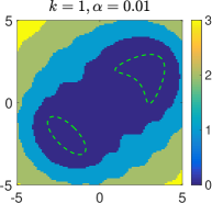
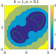
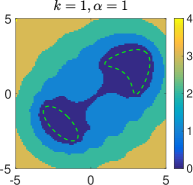
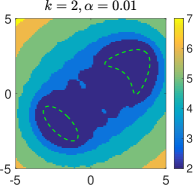
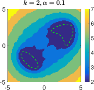
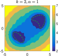
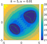
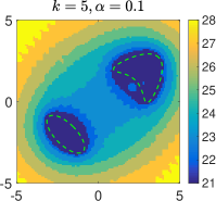
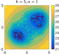
Figure 6.1: Scatterers with positive contrast functions: Visualization of the indicator function $I_{\alpha}$ for three different parameters $\alpha=0.01,0.1$, and $\alpha=1$ (left to right) and three different wave numbers $k=1,2$, and $k=5$ (top down). Exact shape of the scatterers is shown as dashed lines.

We consider two penetrable scatterers, a kite and an ellipse, with positive constant contrast functions $q=1$ (kite) and $q=2$ (ellipse) as sketched in Figure 6.1 (dashed lines), and simulate the corresponding far field matrix ${\bm{F}}_{q}\in{\mathbb{C}}^{64\times 64}$ for $N=64$ observation and incident directions as in (6.1) using a Nyström method for a boundary integral formulation of the scattering problem with three different wave numbers $k=1,2$, and $k=5$.

In Figure 6.1, we show color coded plots of the indicator function $I_{\alpha}$ from (6.6) with threshold parameter $\delta=10^{-14}$ (i.e., the number of negative eigenvalues smaller than $-\delta=-10^{-14}$ of the matrix ${\bm{A}}_{P_{j}}$ from (6.5) on each pixel $P_{j}$) in the region of interest ${[-5,5]^{2}\subseteq{\mathbb{R}}^{2}}$ for three different parameters $\alpha=0.01,0.1$, and $\alpha=1$ (left to right) and three different wave numbers $k=1,2$, and $k=5$ (top down). The equidistant rectangular sampling grid on the region of interest from (6.4) consists of $100$ pixels in each direction.

Overall, the number of negative eigenvalues of the matrix ${\bm{A}}_{P_{j}}$ increases with increasing wave number, and it is larger on pixels $P_{j}$ sufficiently far away from the support of the scatterers than on pixels $P_{j}$ inside, as suggested by Theorems Theorem–Theorem. The lower value always coincides with the number of negative eigenvalues of the real part $\operatorname{Re}({\bm{F}}_{q})$ of the far field matrix from (6.2) that are smaller than the threshold $-\delta$. The number of eigenvalues of ${\bm{A}}_{P_{j}}$, $j=1,\ldots,J$, whose absolute values are larger than $\delta$ is approximately (on average) $25$ (for $k=1$), $36$ (for $k=2$), and $62$ (for $k=5$), independent of $\alpha$.

If the parameter $\alpha$ is suitably chosen, depending on the wave number, then the lowest level set of the indicator function $I_{\alpha}$ nicely approximates the support of the two scatterers. $\lozenge$

Example.

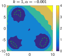
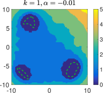
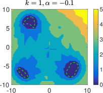
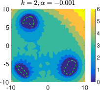
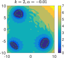
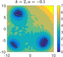
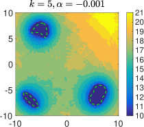
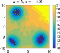
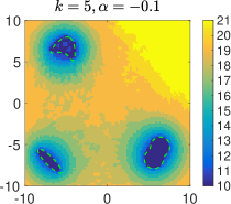
Figure 6.2: Scatterers with negative contrast functions: Visualization of the indicator function $I_{\alpha}$ for three different parameters $\alpha=-0.001,-0.01$, and $\alpha=-0.1$ (left to right) and three different wave numbers $k=1,2$, and $k=5$ (top down). Exact shape of the scatterers is shown as dashed lines.

In the second example, we consider three penetrable scatterers, a kite, an ellipse and a nut-shaped scatterer, with negative constant contrasts $q=-0.8$ (kite), $q=-0.4$ (nut), and $q=-0.2$ (ellipse) as sketched in Figure 6.2 (dashed lines), and simulate the corresponding far field matrix ${\bm{F}}_{q}\in{\mathbb{C}}^{128\times 128}$ for $N=128$ observation and incident directions for three different wave numbers $k=1,2$, and $k=5$. We increase the number of discretization points because the diameter of the support of this configuration of scattering objects is roughly twice as large as in the previous example (i.e., to fulfill the sampling condition (6.3)).

In Figure 6.1, we show color coded plots of the indicator function $I_{\alpha}$ from (6.6) with threshold parameter $\delta=10^{-14}$ in the region of interest ${[-10,10]^{2}\subseteq{\mathbb{R}}^{2}}$ for three different parameters $\alpha=-0.001,-0.01$, and $\alpha=-0.1$ (left to right) and three different wave numbers $k=1,2$, and $k=5$ (top down). The equidistant rectangular sampling grid on the region of interest from (6.4) on this region of interest consists of $100$ pixels in each direction.

Again, the number of negative eigenvalues of the matrix ${\bm{A}}_{P_{j}}$ increases with increasing wave number, and it is larger on pixels $P_{j}$ sufficiently far away from the support of the scatterers than on pixels $P_{j}$ inside, in compliance with Theorems Theorem–Theorem. The lower value always coincides with the number of positive eigenvalues of the matrix $\operatorname{Re}({\bm{F}}_{q})$ from (6.2) that are larger than the threshold $\delta=10^{-14}$. The number of eigenvalues of ${\bm{A}}_{P_{j}}$, $j=1,\ldots,J$, whose absolute values are larger than $\delta$ is approximately (on average) $39$ (for $k=1$), $60$ (for $k=2$), and $115$ (for $k=5$), independent of $\alpha$.

If the parameter $\alpha$ is suitably chosen, depending on the wave number, then the support of the indicator function $I_{\alpha}$ approximates the support of the three scatterers rather well. $\lozenge$

An efficient and suitably regularized numerical implementation of the theoretical results developed in Theorems Theorem–Theorem is beyond the scope of this article, and the preliminary algorithm discussed in this section cannot be considered competitive when compared against state-of-the-art implementations of linear sampling or factorization methods. The numerical results in the Examples Example–Example have been obtained for highly accurate simulated far field data. Further numerical tests showed that the algorithm is rather sensitive to noise in the data.

Conclusions

We have derived new monotonicity relations for the far field operator for the inverse medium scattering problem with compactly supported scattering objects, and we used them to provide novel monotonicity tests to determine the support of unknown scattering objects from far field observations of scattered waves corresponding to infinitely many plane wave incident fields. Along the way we have shown the existence of localized wave functions that have arbitrarily large norm in some prescribed region while having arbitrarily small norm in some other prescribed region.

When compared to traditional qualitative reconstructions methods, advantages of these new characterizations are that they apply to indefinite scattering configurations. Moreover, these characterizations are independent of transmission eigenvalues. However, although we presented some preliminary numerical examples for the sign definite case, a stable numerical implementation of these monotonicity tests still needs to be developed.

empty page

35R30, 65N21

1 An error in the proof of Theorem 5.3 in [3]

At the end of the proof of Theorem 5.3 in GriHar18 “Applying Theorem 4.5 with $D={B_{R}(0)}\setminus\overline{O}$, $q_{1}=0$, and $q_{2}=q$ …” is not possible, because the assumption of Theorem 4.5 in GriHar18 that $q_{1}(x)=q_{2}(x)$ for a.e. $x\in{{\mathbb{R}}^{d}}\setminus\overline{D}$ is not satisfied for this choice of $D$, $q_{1}$ and $q_{2}$.

To fix this issue we will extend the results on localized wave functions from Section 4 of GriHar18 in Section 2 below. Then, in Section 3 we will reformulate Theorem 5.3 of GriHar18, making stronger assumptions on the domains and on the index of refraction, and we will correct the final argument in the original proof in GriHar18.

2 Simultaneously localized wave functions

We establish the existence of simultaneously localized wave functions that have arbitrarily large norm on some prescribed region $E\subseteq{{\mathbb{R}}^{d}}$ while at the same time having arbitrarily small norm in a different region $M\subseteq{{\mathbb{R}}^{d}}$, assuming among others that ${{\mathbb{R}}^{d}}\setminus(\overline{E}\cup\overline{M})$ is connected. The result generalizes Theorem 4.1 in GriHar18 in the sense that we not only control the total field but also the incident field. Similar results have recently been established for the Schrödinger equation in [Thm. 3.11]harrach2020monotonicity and for the Helmholtz obstacle scattering problem in [Thm. 4.5]AlbGri20.

Theorem.

Suppose that $q\in{{L^{\infty}_{0,+}}({{\mathbb{R}}^{d}})}$, and let $E,M\subseteq{{\mathbb{R}}^{d}}$ be open and Lipschitz bounded such that $\operatorname{supp}(q)\subseteq\overline{E}\cup\overline{M}$, ${{\mathbb{R}}^{d}}\setminus(\overline{E}\cup\overline{M})$ is connected, and $E\cap M=\emptyset$. Assume furthermore that there is a connected subset $\Gamma\subseteq\partial E\setminus\overline{M}$ that is relatively open and $C^{1,1}$ smooth.

Then for any finite dimensional subspace $V\subseteq{L^{2}({S^{d-1}})}$ there exists a sequence $(g_{m})_{m\in{\mathbb{N}}}\subseteq{V^{\perp}}$ such that

$$\int_{E}|u_{q,g_{m}}|^{2}\,\operatorname{d\!}x\to\infty\qquad\text{and}\qquad\int_{M}\bigl{(}|u_{q,g_{m}}|^{2}+|u^{i}_{g_{m}}|^{2}\bigr{)}\,\operatorname{d\!}x\to 0\qquad\text{as }m\to\infty\,,$$

where $u^{i}_{g_{m}},u_{q,g_{m}}\in{H^{1}_{\mathrm{loc}}({{\mathbb{R}}^{d}})}$ are given by (2.8a)–(2.8b) in GriHar18 with $g=g_{m}$.

The proof of Theorem Theorem relies on the following three lemmas.

Lemma.

Suppose that $q\in{{L^{\infty}_{0,+}}({{\mathbb{R}}^{d}})}$, let $n^{2}=1+q$, and assume that $D\subseteq{{\mathbb{R}}^{d}}$ is open and bounded. We define

$$L_{q,D}:{L^{2}({S^{d-1}})}\to H^{1}(D)\,,\quad g\mapsto u_{q,g}|_{D}\,,$$

where $u_{q,g}\in{H^{1}_{\mathrm{loc}}({{\mathbb{R}}^{d}})}$ is given by (2.8b) in GriHar18. Then $L_{q,D}$ is a linear operator and its adjoint is given by

$$L_{q,D}^{*}:H^{1}(D)^{*}\to{L^{2}({S^{d-1}})}\,,\quad f\mapsto\mathcal{S}_{q}^{*}w^{\infty}\,,$$

where $H^{1}(D)^{*}$ is the dual of $H^{1}(D)$, $\mathcal{S}_{q}^{*}$ denotes the adjoint of the scattering operator from (2.7) in GriHar18, and ${w^{\infty}\in{L^{2}({S^{d-1}})}}$ is the far field pattern of the radiating solution ${w\in{H^{1}_{\mathrm{loc}}({{\mathbb{R}}^{d}})}}$ to

(2.1) $$\Delta w+k^{2}n^{2}w\,=\,-f\qquad\text{in }{{\mathbb{R}}^{d}}\,.$$

Proof.

This follows from the same arguments that have been used in the proof of Lemma 4.2 in GriHar18.

Lemma.

Suppose that $q\in{{L^{\infty}_{0,+}}({{\mathbb{R}}^{d}})}$, and let $E,M\subseteq{{\mathbb{R}}^{d}}$ be open and Lipschitz bounded such that $\operatorname{supp}(q)\subseteq\overline{E}\cup\overline{M}$, ${{\mathbb{R}}^{d}}\setminus(\overline{E}\cup\overline{M})$ is connected, and $E\cap M=\emptyset$. Assume furthermore that there is a connected subset $\Gamma\subseteq\partial E\setminus\overline{M}$ that is relatively open and $C^{1,1}$ smooth. Then,

$$\mathcal{R}(L_{q,E}^{*})\not\subseteq\mathcal{R}\bigl{(}\begin{pmatrix}L_{q,M}^{*}&L_{0,M}^{*}\end{pmatrix}\bigr{)}$$

and there exists an infinite dimensional subspace $Z\subseteq\mathcal{R}(L_{q,E}^{*})$ such that

$$Z\cap\mathcal{R}\bigl{(}\begin{pmatrix}L_{q,M}^{*}&L_{0,M}^{*}\end{pmatrix}\bigr{)}\,=\,\{0\}\,.$$

Proof.

Let $h\in\mathcal{R}(L_{q,E}^{*})\cap\mathcal{R}\bigl{(}\begin{pmatrix}L_{q,M}^{*}&L_{0,M}^{*}\end{pmatrix}\bigr{)}$. Then Lemma Lemma shows that there exist $f_{q,E}\in H^{1}(E)^{*}$ and $f_{q,M},f_{0,M}\in H^{1}(M)^{*}$ such that the far field patterns $w^{\infty}_{q,E},w^{\infty}_{q,M},w^{\infty}_{0,M}$ of the radiating solutions $w_{q,E},w_{q,M},w_{0,M}\in{H^{1}_{\mathrm{loc}}({{\mathbb{R}}^{d}})}$ to

$$\Delta w_{q,E}+k^{2}(1+q)w_{q,E} \,=\,-f_{q,E} \text{in }{{\mathbb{R}}^{d}}\,,$$

$$\Delta w_{q,M}+k^{2}(1+q)w_{q,M} \,=\,-f_{q,M} \text{in }{{\mathbb{R}}^{d}}\,,$$

$$\Delta w_{0,M}+k^{2}w_{0,M} \,=\,-f_{0,M} \text{in }{{\mathbb{R}}^{d}}\,,$$

satisfy

$$h\,=\,\mathcal{S}_{q}^{*}w^{\infty}_{q,E}\,=\,w^{\infty}_{0,M}+\mathcal{S}_{q}^{*}w^{\infty}_{q,M}\,.$$

Here we used that $\mathcal{S}_{0}$ is the identity operator. Accordingly, using the definition of the scattering operator in (2.7) of GriHar18, we find that

$$\begin{split}0&\,=\,w^{\infty}_{q,E}-w^{\infty}_{q,M}-\mathcal{S}_{q}w^{\infty}_{0,M}\\ &\,=\,w^{\infty}_{q,E}-w^{\infty}_{q,M}-w^{\infty}_{0,M}-2\mathrm{i}k|C_{d}|^{2}F_{q}w^{\infty}_{0,M}\\ &\,=\,w^{\infty}_{q,E}-(w^{\infty}_{q,M}+w^{\infty}_{0,M}+v^{\infty}_{q})\,,\end{split}$$

where $v^{\infty}_{q}$ is the far field of a radiating solution $v_{q}\in{H^{1}_{\mathrm{loc}}({{\mathbb{R}}^{d}})}$ to

$$\Delta v_{q}+k^{2}(1+q)v_{q}\,=\,0\qquad\text{in }{{\mathbb{R}}^{d}}\,.$$

Since $\operatorname{supp}(q)\subseteq\overline{E}\cup\overline{M}$ and ${{\mathbb{R}}^{d}}\setminus(\overline{E}\cup\overline{M})$ is connected, Rellich’s lemma and unique continuation guarantee that

(2.2) $$w_{q,E}-(w_{q,M}+w_{0,M}+v_{q})\,=\,0\qquad\text{in }{{\mathbb{R}}^{d}}\setminus(\overline{E}\cup\overline{M})$$

(cf., e.g., [Thm. 2.14]erratumcolton2013inverse).

Next we discuss the regularity of the traces of $w_{q,E}$ and $w_{q,M}+w_{0,M}+v_{q}$ at the boundary segment $\Gamma\subseteq\partial E\setminus\overline{M}$. W.l.o.g. we may assume that $\Gamma$ is bounded away from $\overline{M}$. Since $\operatorname{supp}(f_{q,M}+f_{0,M})\subseteq\overline{M}$, interior regularity results (see, e.g., [Thm. 4.18]McL00) show that $(w_{q,M}+w_{0,M}+v_{q})\big{|}_{\Gamma}\in H^{\frac{3}{2}}(\Gamma)$. Thus (2.2) implies that $w_{q,E}\big{|}_{\Gamma}^{+}\in H^{\frac{3}{2}}(\Gamma)$ as well.

On the other hand, let $\widetilde{H}^{\frac{1}{2}}(\Gamma)$ be the closure of $\mathcal{D}(\Gamma)$ in $H^{\frac{1}{2}}(\Gamma)$ (see, e.g., [p. 99]McL00). We will construct sources $f\in H^{1}(E)^{*}$ such that $L_{q,E}^{*}f\not\in\mathcal{R}\bigl{(}\begin{pmatrix}L_{q,M}^{*}&L_{0,M}^{*}\end{pmatrix}\bigr{)}$. Given any $g\in\widetilde{H}^{\frac{1}{2}}(\Gamma)$, we denote by $\widetilde{g}\in H^{\frac{1}{2}}(\partial E)$ its extension to $\partial E$ by zero. Accordingly, let $u^{+}\in H^{1}_{\mathrm{loc}}({{\mathbb{R}}^{d}}\setminus\overline{E})$ be the radiating solution to the exterior Dirichlet problem

(2.3) $$\Delta u^{+}+k^{2}n^{2}u^{+}\,=\,0\quad\text{in ${{\mathbb{R}}^{d}}\setminus\overline{E}$}\,,\qquad u^{+}\,=\,\widetilde{g}\quad\text{ on $\partial E$}\,.$$

Similarly, we define $u^{-}\in H^{1}(E)$ as the solution to the interior Dirichlet problem

$$\Delta u^{-}\,=\,0\quad\text{in $E$}\,,\qquad u^{-}\,=\,\widetilde{g}\quad\text{ on $\partial E$}\,.$$

Therewith we introduce $u\in L^{2}_{\mathrm{loc}}({{\mathbb{R}}^{d}})$ by

$$u\,:=\,\begin{cases}u^{-}&\text{in }E\,,\\ u^{+}&\text{in }{{\mathbb{R}}^{d}}\setminus\overline{E}\,,\end{cases}$$

and $f\in H^{1}(E)^{*}$ by

$$f\,:=\,-k^{2}n^{2}u^{-}-\gamma^{*}\Bigl{(}\frac{\partial u}{\partial\nu}\Big{|}_{\partial E}^{+}-\frac{\partial u}{\partial\nu}\Big{|}_{\partial E}^{-}\Bigr{)}\,,$$

where $\gamma^{*}:H^{-\frac{1}{2}}(\partial E)\to H^{1}(E)^{*}$ denotes the adjoint of the interior trace operator $\gamma:H^{1}(E)\to H^{\frac{1}{2}}(\partial E)$. Then $u\in H^{1}_{\mathrm{loc}}({{\mathbb{R}}^{d}})$ (see, e.g., [Lmm. 5.3]Mon03), and

$$\Delta u+k^{2}n^{2}u\,=\,-f\quad\text{in ${{\mathbb{R}}^{d}}$}$$

(see, e.g., [Lmm. 6.9]McL00). Accordingly, $L_{q,E}^{*}f=\mathcal{S}_{q}^{*}u^{\infty}$, where $u^{\infty}\in{L^{2}}({S^{d-1}})$ coincides with the far field of the radiating solution $u^{+}$ to the exterior Dirichlet problem (2.3). If $\widetilde{g}\not\in H^{\frac{3}{2}}(\partial E)$, then our regularity considerations above show that $L_{q,E}^{*}f\not\in\mathcal{R}\bigl{(}\begin{pmatrix}L_{q,M}^{*}&L_{0,M}^{*}\end{pmatrix}\bigr{)}$.

Now let $X\subseteq\widetilde{H}^{\frac{1}{2}}(\Gamma)$ be an infinite dimensional subspace of $\widetilde{H}^{\frac{1}{2}}(\Gamma)$ such that $X\cap H^{\frac{3}{2}}(\Gamma)=\{0\}$ (e.g., the subspace of piecewise linear functions on $\Gamma$ that vanish on $\partial\Gamma$ as considered in the proof of Lemma 4.6 in AlbGri20). Let $G_{E}:H^{\frac{1}{2}}(\Gamma)\to L^{2}({S^{d-1}})$ be the operator that maps $g\in H^{\frac{1}{2}}(\Gamma)$ to the far field pattern of the radiating solution $u^{+}$ of (2.3), where $\widetilde{g}\in H^{\frac{1}{2}}(\partial E)$ is again the extension of $g$ to $\partial E$ by zero. Then $G_{E}$ is one-to-one (see, e.g., [Thm. 3.2]AlbGri20), and thus $Z:=\mathcal{S}_{q}^{*}G_{E}(X)$ is infinite dimensional. Furthermore, we have just shown that

$$Z\subseteq\mathcal{R}(L_{q,E}^{*})\qquad\text{and}\qquad Z\cap\mathcal{R}\bigl{(}\begin{pmatrix}L_{q,M}^{*}&L_{0,M}^{*}\end{pmatrix}\bigr{)}\,=\,\{0\}\,.$$

In the next lemma we quote a special case of Lemma 2.5 in erratumharrach2013monotonicity.

Lemma.

Let $X,Y$ and $Z$ be Hilbert spaces, and let $A:X\to Y$ and $B:X\to Z$ be bounded linear operators. Then,

$$\exists C>0:\;\|Ax\|\leq C\|Bx\|\quad\forall x\in X\qquad\text{if and only if}\qquad\mathcal{R}(A^{*})\subseteq\mathcal{R}(B^{*})\,.$$

Now we give the proof of Theorem Theorem.

Proof (Proof of Theorem Theorem).

Let $V\subseteq{L^{2}({S^{d-1}})}$ be a finite dimensional subspace. We denote by $P_{V}:{L^{2}({S^{d-1}})}\to{L^{2}({S^{d-1}})}$ the orthogonal projection on $V$. Combining Lemma Lemma with a simple dimensionality argument (see [Lmm. 4.7]erratumharrach2017monotonicity) shows that

$$Z\,\not\subseteq\,\mathcal{R}\bigl{(}\begin{pmatrix}L_{q,M}^{*}&L_{0,M}^{*}\end{pmatrix}\bigr{)}+V\,=\,\mathcal{R}(\begin{pmatrix}L_{q,M}^{*}&L_{0,M}^{*}&P_{V}\end{pmatrix})\,,$$

where $Z\subseteq\mathcal{R}(L_{q,E}^{*})$ denotes the subspace in Lemma Lemma. Thus,

$$\mathcal{R}(L_{q,E}^{*})\,\not\subseteq\,\mathcal{R}\bigl{(}\begin{pmatrix}L_{q,M}^{*}&L_{0,M}^{*}\end{pmatrix}\bigr{)}+V\,=\,\mathcal{R}(\begin{pmatrix}L_{q,M}^{*}&L_{0,M}^{*}&P_{V}\end{pmatrix})\,,$$

and accordingly Lemma Lemma implies that there is no constant $C>0$ such that

$$\begin{split}\|L_{q,E}g\|^{2}_{{L^{2}}(E)}&\,\leq\,C^{2}\biggl{\|}\begin{pmatrix}L_{q,M}\\ L_{0,M}\\ P_{V}\end{pmatrix}g\biggr{\|}^{2}_{{L^{2}}(M)\times{L^{2}}(M)\times{L^{2}}({S^{d-1}})}\\ &\,=\,C^{2}\bigl{(}\|L_{q,M}g\|^{2}_{{L^{2}}(M)}+\|L_{0,M}g\|^{2}_{{L^{2}}(M)}+\|P_{V}g\|^{2}_{{L^{2}}({S^{d-1}})}\bigr{)}\end{split}$$

for all $g\in{L^{2}({S^{d-1}})}$. Hence, there exists as sequence $({\widetilde{g}}_{m})_{m\in{\mathbb{N}}}\subseteq{L^{2}({S^{d-1}})}$ such that

$$\begin{split}\|L_{q,E}{\widetilde{g}}_{m}\|_{{L^{2}}(E)}&\to\infty\,,\\ \|L_{q,M}{\widetilde{g}}_{m}\|_{{L^{2}}(M)}+\|L_{0,M}{\widetilde{g}}_{m}\|_{{L^{2}}(M)}+\|P_{V}{\widetilde{g}}_{m}\|_{{L^{2}({S^{d-1}})}}&\to 0\qquad\text{as }m\to\infty\,.\end{split}$$

Setting $g_{m}:={\widetilde{g}}_{m}-P_{V}{\widetilde{g}}_{m}\in{V^{\perp}}\subseteq{L^{2}({S^{d-1}})}$ for any $m\in{\mathbb{N}}$, we finally obtain

$$\|L_{q,E}g_{m}\|_{{L^{2}}(E)}\,\geq\,\|L_{q,E}{\widetilde{g}}_{m}\|_{{L^{2}}(E)}-\|L_{q,E}\|\|P_{V}{\widetilde{g}}_{m}\|_{{L^{2}({S^{d-1}})}}\,\to\,\infty\qquad\text{as }m\to\infty\,,$$

and

$$\|L_{q,M}g_{m}\|_{{L^{2}}(M)}+\|L_{0,M}g_{m}\|_{{L^{2}}(M)}\,\leq\,\|L_{q,M}{\widetilde{g}}_{m}\|_{{L^{2}}(M)}+\|L_{0,M}{\widetilde{g}}_{m}\|_{{L^{2}}(M)}\\ +(\|L_{q,M}\|+\|L_{0,M}\|)\|P_{V}{\widetilde{g}}_{m}\|_{{L^{2}({S^{d-1}})}}\,\to\,0\qquad\text{as }m\to\infty\,.$$

Since $L_{q,E}g_{m}=u_{q,g_{m}}|_{E}$, $L_{q,M}g_{m}=u_{q,g_{m}}|_{M}$, and $L_{0,M}g_{m}=u^{i}_{g_{m}}|_{M}$, this ends the proof.

3 Correction of the statement and of the proof of Theorem 5.3 in [3]

Theorem.

Let $B,D\subseteq{{\mathbb{R}}^{d}}$ be open and Lipschitz bounded such that $\partial D$ is piecewise $C^{1,1}$ smooth, and ${\mathbb{R}}^{d}\setminus\overline{B}$ as well as ${\mathbb{R}}^{d}\setminus\overline{D}$ are connected. Let ${q\in{{L^{\infty}_{0,+}}({{\mathbb{R}}^{d}})}}$ with $\operatorname{supp}(q)=\overline{D}$, and suppose that $-1<q_{\mathrm{min}}\leq q\leq q_{\mathrm{max}}<\infty$ a.e. on $D$ for some constants $q_{\mathrm{min}},q_{\mathrm{max}}\in{\mathbb{R}}$.

Furthermore, we assume that for any point $x\in\partial D$ on the boundary of $D$, there exists a connected unbounded neighborhood $O\subseteq{{\mathbb{R}}^{d}}$ of $x$ such that, for $E:=O\cap D$,

(3.1) $$q|_{E}\geq q_{\mathrm{min},E}>0\qquad\text{or}\qquad q|_{E}\leq q_{\mathrm{max},E}<0$$

for some constants $q_{\mathrm{min},E},q_{\mathrm{max},E}\in{\mathbb{R}}$.

• If $D\subseteq B$, then there exists a constant $C>0$ such that

  $$\alpha T_{B}\,\leq_{\mathrm{fin}}\,\operatorname{Re}(F_{q})\,\leq_{\mathrm{fin}}\,\beta T_{B}\quad\text{for all }\alpha\leq\min\{0,q_{\mathrm{min}}\}\,,\;\beta\geq\max\{0,Cq_{\mathrm{max}}\}\,.$$

• If $D\not\subseteq B$, then

  $$\alpha T_{B}\,\not\leq_{\mathrm{fin}}\,\operatorname{Re}(F_{q})\quad\text{for any }\alpha\in{\mathbb{R}}\quad\text{or}\quad\operatorname{Re}(F_{q})\,\not\leq_{\mathrm{fin}}\,\beta T_{B}\quad\text{for any }\beta\in{\mathbb{R}}\,.$$

Remark.

The assumptions on $B$ and $D$ as well as the local definiteness assumption (3.1) in Theorem Theorem are stronger than in the original version of Theorem 5.3 in GriHar18. $\lozenge$

Proof (Proof of Theorem Theorem).

If $D\subseteq B$, then Corollary 3.4 and Theorem 4.5 in GriHar18 with $q_{1}=0$ and $q_{2}=q$ show that there exists a constant $C>0$ and a finite dimensional subspace $V\subseteq{L^{2}({S^{d-1}})}$ such that, for all $g\in{V^{\perp}}$ and any $\beta\geq\max\{0,Cq_{\mathrm{max}}\}$,

$$\begin{split}\operatorname{Re}\biggl{(}\int_{S^{d-1}}g\,\overline{F_{q}g}\,\operatorname{d\!}s\biggr{)}&\,\leq\,k^{2}\int_{D}q|u_{q,g}|^{2}\,\operatorname{d\!}x\,\leq\,k^{2}q_{\mathrm{max}}\int_{D}|u_{q,g}|^{2}\,\operatorname{d\!}x\\ &\,\leq\,k^{2}Cq_{\mathrm{max}}\int_{D}|u^{i}_{g}|^{2}\,\operatorname{d\!}x\,\leq\,k^{2}\beta\int_{B}|u^{i}_{g}|^{2}\,\operatorname{d\!}x\,.\end{split}$$

Similarly, Theorem 3.2 in GriHar18 with $q_{1}=0$ and $q_{2}=q$ shows that there exists a finite dimensional subspace $V\subseteq{L^{2}({S^{d-1}})}$ such that, for all $g\in{V^{\perp}}$ and any $\alpha\leq\min\{0,q_{\mathrm{min}}\}$,

$$\begin{split}\operatorname{Re}\biggl{(}\int_{S^{d-1}}g\,\overline{F_{q}g}\,\operatorname{d\!}s\biggr{)}&\,\geq\,k^{2}\int_{D}q|u^{i}_{g}|^{2}\,\operatorname{d\!}x\,\geq\,k^{2}q_{\mathrm{min}}\int_{D}|u^{i}_{g}|^{2}\,\operatorname{d\!}x\,\geq\,k^{2}\alpha\int_{B}|u^{i}_{g}|^{2}\,\operatorname{d\!}x\,,\end{split}$$

and part (a) is proven.

We prove part (b) by contradiction. Since $D\not\subseteq B$, $U:=D\setminus B$ is not empty, and there exists $x\in\overline{U}\cap\partial D$ as well as a connected unbounded open neighborhood $O\subseteq{{\mathbb{R}}^{d}}$ of $x$ with $O\cap D\subseteq U$ and $O\cap B=\emptyset$, such that (3.1) is satisfied with $E:=O\cap D$. Furthermore, let $R>0$ be large enough such that $B,D\subseteq{B_{R}(0)}$. Without loss of generality we assume that $O\cap{B_{R}(0)}$, and ${B_{R}(0)}\setminus\overline{O}$ are connected.

We first assume that $q|_{E}\geq q_{\mathrm{min},E}>0$, and that $\operatorname{Re}(F_{q})\leq_{\mathrm{fin}}\beta T_{B}$ for some $\beta\in{\mathbb{R}}$. Using the monotonicity relation (3.1) in Theorem 3.2 of GriHar18 with $q_{1}=0$ and $q_{2}=q$, we find that there exists a finite dimensional subspace $V\subseteq{L^{2}({S^{d-1}})}$ such that, for any $g\in{V^{\perp}}$,

$$\begin{split}0&\,\geq\,\int_{S^{d-1}}g(\overline{\operatorname{Re}(F_{q})g-\beta T_{B}g})\,\operatorname{d\!}s\,\geq\,k^{2}\int_{B_{R}(0)}(q-\beta\chi_{B})|u^{i}_{g}|^{2}\,\operatorname{d\!}x\\ &\,=\,k^{2}\int_{{B_{R}(0)}\setminus\overline{O}}(q-\beta\chi_{B})|u^{i}_{g}|^{2}\,\operatorname{d\!}x+k^{2}\int_{{B_{R}(0)}\cap O}(q-\beta\chi_{B})|u^{i}_{g}|^{2}\,\operatorname{d\!}x\\ &\,\geq\,-k^{2}(\|q\|_{{L^{\infty}}({{\mathbb{R}}^{d}})}+|\beta|)\int_{{B_{R}(0)}\setminus\overline{O}}|u^{i}_{g}|^{2}\,\operatorname{d\!}x+k^{2}q_{\mathrm{min},E}\int_{E}|u^{i}_{g}|^{2}\,\operatorname{d\!}x\,.\end{split}$$

However, this contradicts Theorem 4.1 in GriHar18 with $B=E$, $D={B_{R}(0)}\setminus\overline{O}$, and $q=0$, which guarantees the existence of a sequence $(g_{m})_{m\in{\mathbb{N}}}\subseteq{V^{\perp}}$ with

$$\int_{E}|u^{i}_{g_{m}}|^{2}\,\operatorname{d\!}x\to\infty\qquad\text{and}\qquad\int_{{B_{R}(0)}\setminus\overline{O}}|u^{i}_{g_{m}}|^{2}\,\operatorname{d\!}x\to 0\qquad\text{as }m\to\infty\,.$$

Consequently, $\operatorname{Re}(F_{q})\not\leq_{\mathrm{fin}}\beta T_{B}$ for all $\beta\in{\mathbb{R}}$.

On the other hand, if $q|_{E}\leq q_{\mathrm{max},E}<0$, and if $\alpha T_{B}\leq_{\mathrm{fin}}\operatorname{Re}(F_{q})$ for some $\alpha\in{\mathbb{R}}$, then the monotonicity relation (3.3) in Corollary 3.4 of GriHar18 with $q_{1}=0$ and $q_{2}=q$ shows that there exists a finite dimensional subspace $V\subseteq{L^{2}({S^{d-1}})}$ such that, for any $g\in{V^{\perp}}$,

$$\begin{split}0&\,\leq\,\int_{S^{d-1}}g(\overline{\operatorname{Re}(F_{q})g-\alpha T_{B}g})\,\operatorname{d\!}s\,\leq\,k^{2}\int_{B_{R}(0)}(q|u_{q,g}|^{2}-\alpha\chi_{B}|u^{i}_{g}|^{2})\,\operatorname{d\!}x\\ &\,=\,k^{2}\int_{{B_{R}(0)}\setminus\overline{O}}(q|u_{q,g}|^{2}-\alpha\chi_{B}|u^{i}_{g}|^{2})\,\operatorname{d\!}x+k^{2}\int_{{B_{R}(0)}\cap O}(q|u_{q,g}|^{2}-\alpha\chi_{B}|u^{i}_{g}|^{2})\,\operatorname{d\!}x\\ &\,\leq\,k^{2}q_{\mathrm{max}}\int_{{B_{R}(0)}\setminus\overline{O}}|u_{q,g}|^{2}\,\operatorname{d\!}x+k^{2}|\alpha|\int_{{B_{R}(0)}\setminus\overline{O}}|u^{i}_{g}|^{2}\,\operatorname{d\!}x+k^{2}q_{\mathrm{max},E}\int_{E}|u_{q,g}|^{2}\,\operatorname{d\!}x\,.\end{split}$$

Let $M:={B_{R}(0)}\setminus\overline{O}$. Since $\partial D$ is piecewise $C^{1,1}$ smooth, there is a connected subset $\Gamma\subseteq\partial E\setminus\overline{M}$ that is relatively open and $C^{1,1}$ smooth. Applying Theorem Theorem we find that there exists a sequence $(g_{m})_{m\in{\mathbb{N}}}\subseteq{V^{\perp}}$ such that

$$\int_{E}|u_{q,g_{m}}|^{2}\,\operatorname{d\!}x\to\infty\qquad\text{and}\qquad\int_{{B_{R}(0)}\setminus\overline{O}}|u_{q,g_{m}}|^{2}+|u^{i}_{g_{m}}|^{2}\,\operatorname{d\!}x\to 0\qquad\text{as }m\to\infty\,.$$

However, since $q_{\mathrm{max},E}<0$, this gives a contradiction. Consequently, $\alpha T_{B}\not\leq_{\mathrm{fin}}\operatorname{Re}(F_{q})$ for all $\alpha\in{\mathbb{R}}$, which ends the proof of part (b).

abbrv literaturliste_erratum.bib

References

- [1] L. Arnold and B. Harrach. Unique shape detection in transient eddy current problems. Inverse Problems, 29(9):095004, 2013.
- [2] A. Barth, B. Harrach, N. Hyvönen, and L. Mustonen. Detecting stochastic inclusions in electrical impedance tomography. Inverse Problems, 33(11):115012, 2017.
- [3] T. Brander, B. Harrach, M. Kar, and M. Salo. Monotonicity and enclosure methods for the p-Laplace equation. SIAM J. Appl. Math., accepted for publication.
- [4] M. Brühl. Explicit characterization of inclusions in electrical impedance tomography. SIAM J. Math. Anal., 32(6):1327–1341, 2001.
- [5] F. Cakoni and D. Colton. A qualitative approach to inverse scattering theory. Springer, New York, 2014.
- [6] F. Cakoni, D. Colton, and H. Haddar. Inverse scattering theory and transmission eigenvalues, volume 88 of CBMS-NSF Regional Conference Series in Applied Mathematics. Society for Industrial and Applied Mathematics (SIAM), Philadelphia, PA, 2016.
- [7] F. Cakoni, D. Colton, and P. Monk. The linear sampling method in inverse electromagnetic scattering, volume 80 of CBMS-NSF Regional Conference Series in Applied Mathematics. Society for Industrial and Applied Mathematics (SIAM), Philadelphia, PA, 2011.
- [8] D. Colton and A. Kirsch. A simple method for solving inverse scattering problems in the resonance region. Inverse Problems, 12(4):383–393, 1996.
- [9] D. Colton and R. Kress. Inverse acoustic and electromagnetic scattering theory. Springer, New York, third edition, 2013.
- [10] H. Garde. Comparison of linear and non-linear monotonicity-based shape reconstruction using exact matrix characterizations. Inverse Probl. Sci. Eng., 26(1):33–50, 2018.
- [11] H. Garde and S. Staboulis. Convergence and regularization for monotonicity-based shape reconstruction in electrical impedance tomography. Numer. Math., 135(4):1221–1251, 2017.
- [12] H. Garde and S. Staboulis. The regularized monotonicity method: detecting irregular indefinite inclusions. arXiv preprint arXiv:1705.07372, 2017.
- [13] B. Gebauer. Localized potentials in electrical impedance tomography. Inverse Probl. Imaging, 2(2):251–269, 2008.
- [14] G. H. Golub and C. F. Van Loan. Matrix computations. Johns Hopkins Studies in the Mathematical Sciences. Johns Hopkins University Press, Baltimore, MD, third edition, 1996.
- [15] R. Griesmaier and J. Sylvester. Uncertainty principles for inverse source problems, far field splitting, and data completion. SIAM J. Appl. Math., 77(1):154–180, 2017.
- [16] M. Hanke and A. Kirsch. Sampling methods. In O. Scherzer, editor, Handbook of Mathematical Models in Imaging, pages 501–550. Springer, 2011.
- [17] B. Harrach. On uniqueness in diffuse optical tomography. Inverse Problems, 25(5):055010, 2009.
- [18] B. Harrach. Simultaneous determination of the diffusion and absorption coefficient from boundary data. Inverse Probl. Imaging, 6(4):663–679, 2012.
- [19] B. Harrach. Recent progress on the factorization method for electrical impedance tomography. Comput. Math. Methods Med., page 425184, 2013.
- [20] B. Harrach, E. Lee, and M. Ullrich. Combining frequency-difference and ultrasound modulated electrical impedance tomography. Inverse Problems, 31(9):095003, 2015.
- [21] B. Harrach and Y.-H. Lin. Monotonicity-based inversion of the fractional Schrödinger equation. arXiv preprint arXiv:1711.05641, 2017.
- [22] B. Harrach and M. N. Minh. Enhancing residual-based techniques with shape reconstruction features in electrical impedance tomography. Inverse Problems, 32(12):125002, 2016.
- [23] B. Harrach and M. N. Minh. Monotonicity-based regularization for phantom experiment data in electrical impedance tomography. In B. Hofmann, A. Leitao, and J. P. Zubelli, editors, New Trends in Parameter Identification for Mathematical Models, Trends Math., pages 107–120. Springer International, 2018.
- [24] B. Harrach, V. Pohjola, and M. Salo. Monotonicity and local uniqueness for the Helmholtz equation. arXiv preprint arXiv:1709.08756, 2017.
- [25] B. Harrach and J. K. Seo. Exact shape-reconstruction by one-step linearization in electrical impedance tomography. SIAM J. Math. Anal., 42(4):1505–1518, 2010.
- [26] B. Harrach and M. Ullrich. Monotonicity-based shape reconstruction in electrical impedance tomography. SIAM J. Math. Anal., 45(6):3382–3403, 2013.
- [27] B. Harrach and M. Ullrich. Resolution guarantees in electrical impedance tomography. IEEE Trans. Med. Imaging, 34:1513–1521, 2015.
- [28] B. Harrach and M. Ullrich. Local uniqueness for an inverse boundary value problem with partial data. Proc. Amer. Math. Soc., 145(3):1087–1095, 2017.
- [29] M. Ikehata. Size estimation of inclusion. J. Inverse Ill-Posed Probl., 6(2):127–140, 1998.
- [30] H. Kang, J. K. Seo, and D. Sheen. The inverse conductivity problem with one measurement: stability and estimation of size. SIAM J. Math. Anal., 28(6):1389–1405, 1997.
- [31] A. Kirsch. Characterization of the shape of a scattering obstacle using the spectral data of the far field operator. Inverse Problems, 14(6):1489–1512, 1998.
- [32] A. Kirsch. Factorization of the far-field operator for the inhomogeneous medium case and an application in inverse scattering theory. Inverse Problems, 15(2):413–429, 1999.
- [33] A. Kirsch. The MUSIC algorithm and the factorization method in inverse scattering theory for inhomogeneous media. Inverse Problems, 18(4):1025–1040, 2002.
- [34] A. Kirsch. An introduction to the mathematical theory of inverse problems. Springer, New York, second edition, 2011.
- [35] A. Kirsch. Remarks on the Born approximation and the factorization method. Appl. Anal., 96(1):70–84, 2017.
- [36] A. Kirsch and N. Grinberg. The factorization method for inverse problems. Oxford University Press, Oxford, 2008.
- [37] A. Kirsch and A. Lechleiter. The inside–outside duality for scattering problems by inhomogeneous media. Inverse Problems, 29(10):104011, 2013.
- [38] E. Lakshtanov and A. Lechleiter. Difference factorizations and monotonicity in inverse medium scattering for contrasts with fixed sign on the boundary. SIAM J. Math. Anal., 48(6):3688–3707, 2016.
- [39] A. Lechleiter. The factorization method is independent of transmission eigenvalues. Inverse Probl. Imaging, 3(1):123–138, 2009.
- [40] A. Maffucci, A. Vento, S. Ventre, and A. Tamburrino. A novel technique for evaluating the effective permittivity of inhomogeneous interconnects based on the monotonicity property. IEEE Transactions on Components, Packaging and Manufacturing Technology, 6(9):1417–1427, 2016.
- [41] R. Potthast. A survey on sampling and probe methods for inverse problems. Inverse Problems, 22(2):R1–R47, 2006.
- [42] Z. Su, L. Udpa, G. Giovinco, S. Ventre, and A. Tamburrino. Monotonicity principle in pulsed eddy current testing and its application to defect sizing. In Applied Computational Electromagnetics Society Symposium-Italy (ACES), 2017 International, pages 1–2. IEEE, 2017.
- [43] A. Tamburrino and G. Rubinacci. A new non-iterative inversion method for electrical resistance tomography. Inverse Problems, 18(6):1809–1829, 2002.
- [44] A. Tamburrino, Z. Sua, S. Ventre, L. Udpa, and S. S. Udpa. Monotonicity based imaging method in time domain eddy current testing. Electromagnetic Nondestructive Evaluation (XIX), 41:1, 2016.
- [45] S. Ventre, A. Maffucci, F. Caire, N. Le Lostec, A. Perrotta, G. Rubinacci, B. Sartre, A. Vento, and A. Tamburrino. Design of a real-time eddy current tomography system. IEEE Transactions on Magnetics, 53(3):1–8, 2017.
- [46] L. Zhou, B. Harrach, and J. K. Seo. Monotonicity-based electrical impedance tomography for lung imaging. Inverse Problems, 34(4):045005, 25, 2018.
ERRATUM: MONOTONICITY IN INVERSE MEDIUM SCATTERING ON UNBOUNDED DOMAINS
ROLAND GRIESMAIER111Institut für Angewandte und Numerische Mathematik, Karlsruher Institut für Technologie, 76049 Karlsruhe, Germany ().
and
BASTIAN HARRACH222Institut für Mathematik, Universität Frankfurt, 60325 Frankfurt am Main, Germany ().