Stochastic multiscale flux basis for Stokes-Darcy flows

Abstract

Three algorithms are developed for uncertainty quantification in modeling coupled Stokes and Darcy flows. The porous media may consist of multiple regions with different properties. The permeability is modeled as a non-stationary stochastic variable, with its log represented as a sum of local Karhunen-Loève (KL) expansions. The problem is approximated by stochastic collocation on either tensor-product or sparse grids, coupled with a multiscale mortar mixed finite element method for the spatial discretization. A non-overlapping domain decomposition algorithm reduces the global problem to a coarse scale mortar interface problem, which is solved by an iterative solver, for each stochastic realization. In the traditional domain decomposition implementation, each subdomain solves a local Dirichlet or Neumann problem in every interface iteration. To reduce this cost, two additional algorithms based on deterministic or stochastic multiscale flux basis are introduced. The basis consists of the local flux (or velocity trace) responses from each mortar degree of freedom. It is computed for each subdomain independently before the interface iteration begins. The use of the multiscale flux basis avoids the need for subdomain solves on each iteration. The deterministic basis is computed at each stochastic collocation and used only at this realization. The stochastic basis is formed by further looping over all local realizations of a subdomain’s KL region before the stochastic collocation begins. It is reused over multiple realizations. Numerical tests are presented to illustrate the performance of the three algorithms, with the stochastic multiscale flux basis showing significant savings in computational cost compared to the other two algorithms.

Keywords.  stochastic collocation, domain decomposition, multiscale basis, mortar finite element, mixed finite element, Stokes-Darcy flows

1 Introduction

Coupled Stokes-Darcy flows arise in numerous applications, including interaction between surface and groundwater flows, cardiovascular flows, industrial filtration, fuel cells, and flows in fractured or vuggy reservoirs. The Stokes equations describe the motion of incompressible fluids and the Darcy model describes the infiltration process. In this work we consider mixed velocity-pressure formulations in both regions. The Beavers-Joseph-Saffman slip with friction condition [9, 49] is applied on the Stokes-Darcy interface. Existence and uniqueness of a weak solution has been proved in [42], see also [20] for analysis of the system with a pressure Darcy formulation. The finite element approximation of the coupled problem has been studied extensively, see, e.g., [42, 20, 48, 28] for some of the early works. To the best of our knowledge, all previous studies have considered the deterministic model. Often, due to incomplete knowledge of the physical parameters, quantification of the model uncertainty needs to be incorporated. In this paper, we study the interaction of a free fluid with a porous medium with stochastic permeability. Even though the stochasticity comes only from the uncertain nature of the permeability in the porous region, the resulting solution is stochastic over the entire domain, due to the coupling conditions. We develop algorithms for computing statistical moments of the solution, such as mean, variance, and higher moments.

In this work the permeability function is parameterized using a truncated Karhunen-Loéve (KL) expansion with independent identically distributed random variables as coefficients. Given a covariance relationship with empirically determined statistics, one can compute the eigenvalues and corresponding eigenfunctions that form the KL series. This approach is commonly used for stochastic permeability as shown in [43, 55, 58, 59] and in particular can be used in the framework for stochastic collocation and mixed finite elements [31]. Following [43, 35], we consider non-stationary porous media with different covariance functions in different parts of the domain, which allows for modeling heterogeneous media. For instance, the arrangement of sedimentary rocks in distinct layers motivates the use of such statistically independent regions, each region corresponding to a particular rock type. In this paper such regions are referred to as KL regions. The covariance between two points that lie in different KL regions is zero, while otherwise it depends on the distance between those points.

To compute the statistical moments of the solution, we employ the stochastic collocation method [8, 56, 45, 31], which samples the stochastic space at specifically chosen points. In this work we use zeros of orthogonal polynomials with either tensor product or sparse grid approximations. The method is non-intrusive, since it requires solving a sequence of deterministic problems. In this regard it resembles Monte Carlo Simulation (MCS) [26]. However, MCS may exhibit a high computational cost due to the need to generate valid representative statistics from a large number of realizations at random points in the stochastic event space. In comparison, stochastic collocation provides improved approximation of polynomial interpolation type and thus may result in better accuracy than MCS with fewer realizations. In terms of its approximation properties, stochastic collocation is comparable to polynomial chaos expansions [57] or stochastic finite element methods [19, 36]. However, the intrusive character of these methods may complicate their implementation. In addition, they result in high dimensional algebraic problems with fully coupled physical and stochastic dimensions.

In each stochastic realization we solve the coupled Stokes-Darcy problem using the multiscale mortar mixed finite element method (MMMFEM) introduced in [5, 37, 53]. The MMMFEM decomposes the physical domain into a union of non-overlapping subdomains of Stokes or Darcy type. Any Darcy subdomain is assumed to be contained in only one KL region, but KL regions may contain multiple subdomains. Each subdomain is discretized on a fine scale using stable and conforming mixed finite element spaces of Stokes or Darcy type. The grids are allowed to be non-matching along subdomain interfaces. A mortar space is introduced on the interfaces and discretized on a coarse scale. A coarse scale mortar Lagrange multiplier $\lambda_{H}$ is used to impose weakly continuity of flux. Since we allow for multiple subdomains, we must account for interfaces of Stokes-Darcy, Darcy-Darcy and Stokes-Stokes types. In particular, on Stokes-Darcy or Darcy-Darcy interfaces $\lambda_{H}$ is the normal stress or pressure, respectively - a scalar quantity, and it is used to impose continuity of the normal velocity. On Stokes-Stokes interfaces $\lambda_{H}$ is the normal stress vector, and it is used to impose continuity of the entire velocity vector. Following [38, 53], the global fine scale problem is reduced to a coarse scale interface problem, which can be solved in parallel by Krylov iterative solvers. In the traditional implementation, the action of the interface operator requires solving Neumann problems in Stokes subdomains and Dirichlet problems in Darcy subdomains. The finite element tearing and interconnecting (FETI) method [25, 52] is employed to deal with the possibly singular Stokes subdomain problems. For previous work on domain decomposition for Stokes-Darcy flows in the two-subdomain case, we refer the reader to [21, 22, 39, 29].

The multiscale approximation of the MMMFEM is motivated by the fact that in porous media problems, resolving fine scale accuracy is often computationally infeasible. The method is an alternative to other multiscale methods, such as the variational multiscale method [41, 4] and multiscale finite elements [40, 14, 2, 16, 24, 27, 15]. Both have been applied to stochastic problems in [7, 30] and [23, 1] respectively. The MMMFEM is more flexible than the aforementioned methods, since it allows for a posteriori error estimation and adaptive refinement of the coarse scale mortar interface mesh [5].

In the traditional implementation of the MMMFEM, the dominant computational cost is the solution of Stokes or Darcy subdomain problems at each interface iteration. Even though the dimension of the interface problem is reduced due to the coarse scale mortar space, the cost can be significant and the number of iterations grow with the condition number of the interface operator. To alleviate this cost, we utilize a multiscale flux basis. We follow the approach introduced in [34] for the Darcy problem, extended to the Stokes-Darcy problem in [33], and the stochastic Darcy problem in [35]. In particular, we compute a multiscale basis consisting of the local fine scale flux (or velocity trace) responses from each coarse scale mortar degree of freedom. It is computed for each subdomain independently before the interface iteration begins. The use of the multiscale flux basis avoids the need for subdomain solves on each Krylov iteration, since the action of the interface operator can be computed by a simple linear combination of the basis functions. We develop and compare two multiscale flux basis algorithms for the stochastic Stokes-Darcy problem. In the first method, referred to as deterministic multiscale flux basis, the basis is computed at each stochastic collocation and used only during the interface iteration at this realization. In this approach the number of subdomain solves is proportional to the number of mortar degrees of freedom per subdomain and the total number of stochastic collocation points. In the second method we follow the approach from [35] and explore the fact that the stochastic parameter is represented as a sum of local KL expansions. Unlike the first method, we do not recompute the basis at the beginning of every stochastic collocation. Instead, a full multiscale basis pre-computation is carried out on each subdomain for all local stochastic realizations before the global collocation loop begins. This stochastic basis can be reused multiple times during the collocation loop, since the same local subdomain stochastic structure occurs over multiple realizations. In this method, referred to as stochastic multiscale flux basis, the number of subdomain solves is proportional to the number of mortar degrees of freedom per subdomain and the number of local stochastic collocation points, resulting in additional significant computational savings.

While in this work we focus on single phase flow, extensions to multiphase flow can also be considered. For example, multiscale mixed finite element methods for multiphase flow in porous media have been developed in [3, 2, 32]. Stochastic collocation with mixed finite elements for multiphase Darcy flow have been studied in [31]. While multiphase Stokes-Darcy couplings have been less extensively studied, we refer the reader to [18] for the coupling of the shallow water equations with the Richards equation for modeling unsaturated groundwater flows, as well as [12, 13] for using diffuse interface models for two-phase Stokes-Darcy flows.

The remainder of the paper is organized as follows. The model problem is introduced in Section 2. The MMMFEM is introduced in Section 3. Tensor product and sparse grid stochastic collocation algorithms are presented in Section 4. Three algorithms, including traditional MMMFEM, deterministic and stochastic multiscale flux basis are presented in Section 5. In Section 6, the algorithms are employed in several numerical tests and compared in terms of computational efficiency.

2 Model problem

Let $\Omega$ be a stochastic space with probability measure $P$. For any random variable $\xi(\omega):\Omega\rightarrow\mathbb{R}$, $\xi(w)=z$, with probability density function (PDF) $\rho(z)$, its mean or expectation is defined by

$$E[\xi]=\int_{\Omega}\xi(\omega)dP(\omega)=\int_{\mathbb{R}}z\rho(z)dz,$$ (1)

and its variance is given by

$$Var[\xi]=E[\xi^{2}]-(E[\xi])^{2}.$$

We denote the fluid region and the porous media region by $D_{s}\subset\mathbb{R}^{d}$ and $D_{d}\subset\mathbb{R}^{d}$, respectively, where $d=2,3$. Each region may consists of several non-connected components. Let $\Gamma_{s}$ be the outside boundary of $D_{s}$ and let ${\bf n}_{s}$ be the outward unit normal vector on $\partial D_{s}$. Let $\Gamma_{d}$ be the outside boundary of $D_{d}$ and let ${\bf n}_{d}$ be the outward unit normal vector on $\partial D_{d}$. The entire physical domain is defined as $D=D_{s}\cup D_{d}$, with the Stokes-Darcy interface denoted by $\Gamma_{sd}=D_{s}\cap D_{d}$. Let $(\mathbf{u}_{s},p_{s})$ and $(\mathbf{u}_{d},p_{d})$ be the velocity and pressure unknowns in the Stokes and Darcy regions, respectively. In the Stokes region, let $\nu_{s}$ be the viscosity coefficient and define the deformation rate tensor ${\bf D}$ and stress tensor ${\bf T}$ by

$$\mathbf{D}(\mathbf{u}_{s}):=\frac{1}{2}(\nabla\mathbf{u}_{s}+(\nabla\mathbf{u}_{s})^{T}),\quad\mathbf{T}(\mathbf{u}_{s},p_{s}):=-p_{s}\mathbf{I}+2\nu_{s}\mathbf{D}(\mathbf{u}_{s}).$$

In the Darcy region, let $\nu_{d}$ be the viscosity coefficient and $K(\mathbf{x},\omega)$ be a stochastic function defined on $D\times\Omega$ representing the non-stationary permeability of the porous medium. We assume $K$ to be uniformly positive definite for $P$-almost every $\omega\in\Omega$ with components in $L^{\infty}(D_{d})$. The coupled Stokes-Darcy flow model is as follows. For $P$-almost every $\omega\in\Omega$, in the Stokes region, $(\mathbf{u}_{s},p_{s})$ satisfy

$$-\nabla\cdot{\bf T}(\mathbf{u}_{s},p_{s})\equiv-2\nu_{s}\nabla\cdot{\bf D}(\mathbf{u}_{s})+\nabla p_{s} =\mathbf{f}_{s}\quad\text{in }D_{s},$$ (2)

$$\nabla\cdot\mathbf{u}_{s} =0\quad\text{in }D_{s},$$ (3)

$$\mathbf{u}_{s} ={\bf 0}\quad\text{on }\Gamma_{s},$$ (4)

where $\mathbf{f}_{s}$ represents the body force. In the Darcy region, $(\mathbf{u}_{d},p_{d})$ satisfy

$$\nu_{d}K(\mathbf{x},\omega)^{-1}\mathbf{u}_{d}+\nabla p_{d} =\mathbf{f}_{d}\quad\text{in }D_{d},$$ (5)

$$\nabla\cdot\mathbf{u}_{d} =q_{d}\quad\text{in }D_{d},$$ (6)

$$\mathbf{u}_{d}\cdot\mathbf{n}_{d} =0\quad\text{on }\Gamma_{d},$$ (7)

where $\mathbf{f}_{d}$ is the gravity force and $q_{d}$ is an external source or sink term satisfying the solvability condition

$$\int_{D_{d}}q_{d}\ d\mathbf{x}=0.$$

The two models are coupled on $\Gamma_{sd}$ through the following interface conditions:

$$\mathbf{u}_{s}\cdot\mathbf{n}_{s}+\mathbf{u}_{d}\cdot\mathbf{n}_{d} =0\quad\text{on }\Gamma_{sd},$$ (8)

$$-({\bf T}(\mathbf{u}_{s},p_{s})\mathbf{n}_{s})\cdot\mathbf{n}_{s}\equiv p_{s}-2\nu_{s}({\bf D}(\mathbf{u}_{s})\mathbf{n}_{s})\cdot\mathbf{n}_{s} =p_{d}\quad\text{on }\Gamma_{sd},$$ (9)

$$-({\bf T}(\mathbf{u}_{s},p_{s})\mathbf{n}_{s})\cdot\mbox{\boldmath$\tau$}_{l}\equiv-2\nu_{s}({\bf D}(\mathbf{u}_{s})\mathbf{n}_{s})\cdot\mbox{\boldmath$\tau$}_{l} =\frac{\nu_{s}\alpha}{\sqrt{K_{l}}}\mathbf{u}_{s}\cdot\mbox{\boldmath$\tau$}_{l},\,\,1\leq l\leq d-1\text{ on }\Gamma_{sd}.$$ (10)

Conditions (8) and (9) denote the continuity of flux and normal stress through $\Gamma_{sd}$, respectively. Condition (10) is the well-known Beaver-Joseph-Saffman slip with friction law [9, 49], where $\{\mbox{\boldmath$\tau$}_{l}\}_{l=1}^{d-1}$ is an orthogonal system of unit tangent vectors on $\Gamma_{sd}$ and $K_{l}=(K(\mathbf{x},\omega)\mbox{\boldmath$\tau$}_{l})\cdot\mbox{\boldmath$\tau$}_{l}$. The constant $\alpha>0$ is a friction coefficient determined experimentally.

2.1 Multi-region Karhunen-Loève (KL) expansion

Let $Y(\mathbf{x},\omega)=\ln(K(\mathbf{x},\omega))$ be the log permeability and define

$$Y^{\prime}(\mathbf{x},\omega):=Y(\mathbf{x},\omega)-E[Y](\mathbf{x}).$$

We assume that the Darcy region $D_{d}$ is a union of several non-overlapping KL regions $D_{d}=\bigcup_{i=1}^{N_{\Omega}}D_{KL}^{(i)}$, where the stochastic structure of every region is independent from the others. In other words, the covariance between any pair of points from different KL regions is zero. The permeability in each region is parameterized by a local KL expansion. The global stochastic space is decomposed correspondingly by

$$\Omega=\bigotimes_{i=1}^{N_{\Omega}}\Omega^{(i)}.$$

Therefore, for each event $\omega\in\Omega$, we can write $\omega=(\omega^{(1)},\ldots,\omega^{(N_{\Omega})})$ and

$$Y^{\prime}(\mathbf{x},\omega)=\sum_{i=1}^{N_{\Omega}}Y^{(i)}(\mathbf{x},\omega^{(i)}).$$

Each $Y^{(i)}$ has a physical support in $D_{KL}^{(i)}$ with a covariance function

$$C_{Y^{(i)}}(\mathbf{x},\mathbf{\bar{x}})=E[Y^{(i)}(\mathbf{x},\omega^{(i)})Y^{(i)}(\mathbf{\bar{x}},\omega^{(i)})].$$

Since the covariance function is symmetric and positive definite, it can be decomposed into the series expansion

$$C_{Y^{(i)}}(\mathbf{x},\mathbf{\bar{x}})=\sum_{j=1}^{\infty}\lambda_{j}^{(i)}f_{j}^{(i)}(\mathbf{x})f_{j}^{(i)}(\mathbf{\bar{x}}),$$

where the eigenvalues and eigenfunctions $\lambda_{j}^{(i)}$, $f_{j}^{(i)}$ respectively, are computed by using $C_{Y^{(i)}}$ as the kernel of Fredholm integral equation

$$\int_{D_{KL}^{(i)}}C_{Y^{(i)}}(\mathbf{x},\mathbf{\bar{x}})f_{j}^{(i)}(\mathbf{x})d\mathbf{x}=\lambda_{j}^{(i)}f_{j}^{(i)}(\mathbf{\bar{x}}).$$ (11)

The eigenfunctions of $C_{Y^{(i)}}$ are mutually orthogonal and form a complete spanning set. Therefore the Karhunen-Loève expansion for the log permeability can be expressed as

$$Y^{\prime}(\mathbf{x},\omega)=\sum_{i=1}^{N_{\Omega}}~{}\sum_{j=1}^{\infty}~{}\xi_{j}^{(i)}(\omega^{(i)})\sqrt{\lambda_{j}^{(i)}}f_{j}^{(i)}(\mathbf{x}),$$ (12)

where the eigenfunctions $f_{j}^{(i)}(\mathbf{x})$ computed in (11) have been extended by zero outside of $D_{KL}^{(i)}$ and $\xi_{j}^{(i)}:\Omega_{i}\to\mathbb{R}$ are independent identically distributed random variables [36]. We assume that $Y^{(i)}$ is Gaussian, so each $\xi_{j}^{(i)}$ is a random variable with zero mean and unit variance, with a probability density function $\rho_{j}^{(i)}(y)=\frac{1}{\sqrt{2\pi}}\exp[\frac{-y^{2}}{2}]$.

Since the eigenvalues $\lambda_{j}^{(i)}$ decay rapidly with $j$ [59], it is reasonable to truncate the local KL expansions. If the expansion is truncated prematurely, the permeability may appear too smooth in a particular KL region. In our case, for any KL region $i$, we truncate the expansion after its first $N_{\textrm{term}}(i)$ terms. Increasing $N_{\textrm{term}}(i)$ introduces more heterogeneity into the permeability realizations for a chosen region. It is beyond the scope of this paper to address the modeling error associated with truncating the KL expansion. Some work has been done to quantify the modeling error [45] and it can be reduced a posteriori [11]. The truncation allows us to approximate (12) by

$$Y^{\prime}(\mathbf{x},\omega)\approx\sum_{i=1}^{N_{\Omega}}\sum_{j=1}^{N_{\textrm{term}}(i)}\xi_{j}^{(i)}(\omega^{(i)})\sqrt{\lambda_{j}^{(i)}}f_{j}^{(i)}(\mathbf{x}).$$ (13)

The above also shows that globally we have $N_{\textrm{term}}:=\sum_{i=1}^{N_{\Omega}}N_{\textrm{term}}(i)$ terms in $Y^{\prime}$.

Let $\mathbb{S}_{j}^{(i)}=\xi_{j}^{(i)}(\Omega^{(i)})$ be the images of the random variables. They form finite dimensional spaces that are local to each KL region, $\mathbb{S}^{(i)}=\prod_{j=1}^{N_{\textrm{term}}(i)}\mathbb{S}_{j}^{(i)}\subseteq\mathbb{R}^{N_{\textrm{term}}(i)}$, as well as a global vector space $\mathbb{S}=\prod_{i=1}^{N_{\Omega}}~{}\mathbb{S}^{(i)}\subseteq\mathbb{R}^{N_{\textrm{term}}}$. Let $\kappa$ be a function that provides a natural ordering for the global number of stochastic dimensions. Then the $j$-th stochastic parameter of the $i$-th KL region have a global index in $\{1,\ldots,N_{\textrm{term}}\}$ given by the function

$$\kappa(i,j)=\left\{\begin{tabular}[]{ll}$j$,&if $i=1$,\\ $j+\displaystyle\sum_{k=1}^{i-1}N_{\textrm{term}}(k)$,&if $i>1$.\end{tabular}\right.$$

The joint PDF for $\mathbf{\xi}=(\xi_{j}^{(i)})_{\kappa}$ is $\rho=\prod_{i}\prod_{j}\rho_{j}^{(i)}$. According to (13), we approximate $Y(\mathbf{x},\omega)$ by $Y(\mathbf{x},\mathbf{y})$, where $\mathbf{y}=\left(\xi_{j}^{(i)}(\omega^{(i)})\right)_{\kappa}$. We further note that, since in most cases closed-form eigenfunctions and eigenvalues are not readily available, the integral equation (11) is solved numerically.

3 Multiscale mortar mixed finite element method

3.1 Domain decomposition

The coupled Stokes-Darcy flow problem is solved using domain decomposition method following the approach described in [53]. The Stokes and Darcy domains are partitioned into $N_{s}$ and $N_{d}$ non-overlapping subdomains, respectively. Let $N=N_{s}+N_{d}$, with $D_{s}=\bigcup_{i=1}^{N_{s}}D_{i}$, $D_{d}=\bigcup_{i=N_{s}+1}^{N}D_{i}$, and $D_{i}\cap D_{j}=\emptyset$ for $i\neq j$. Let the interface between adjacent subdomains be $\Gamma_{i,j}=\partial D_{i}\cap\partial D_{j}$. Depending on the models of adjacent domains, we group all interfaces into three different types: Stokes-Stokes type, Darcy-Darcy type and Stokes-Darcy type, denoted by $\Gamma_{ss}$, $\Gamma_{dd}$ and $\Gamma_{sd}$, respectively. The union of all interfaces is defined as $\Gamma=\Gamma_{ss}\bigcup\Gamma_{dd}\bigcup\Gamma_{sd}$. Let $\Gamma_{i}=\partial D_{i}\cap\Gamma$. In addition, it is assumed that in $D_{d}$ each KL region is an exact union of subdomains. Let $(\mathbf{u}_{i},p_{i})=(\mathbf{u}_{s}|_{D_{i}},p_{s}|_{D_{i}})$ if $D_{i}$ is a Stokes subdomain and $(\mathbf{u}_{i},p_{i})=(\mathbf{u}_{d}|_{D_{i}},p_{d}|_{D_{i}})$ if it is a Darcy subdomain.

In addition to the interface conditions (8)–(10) on $\Gamma_{sd}$, we impose continuity of velocity and normal stress on $\Gamma_{ss}$, and continuity of normal velocity and pressure on $\Gamma_{dd}$:

$$[\mathbf{u}]=0,\quad[\mathbf{T}(\mathbf{u},p)\mathbf{n}]=0\quad\textrm{on}~{}\Gamma_{ss},$$ (14)

$$[\mathbf{u}\cdot\mathbf{n}]=0,\quad[p]=0\quad\textrm{on}~{}\Gamma_{dd},$$ (15)

where $[\ \cdot\ ]$ represents the jump on the interface. For example, on $\Gamma_{ij}$, $[\mathbf{u}]=(\mathbf{u}_{i}-\mathbf{u}_{j})|_{\Gamma_{ij}}$, $[\mathbf{u}\cdot\mathbf{n}]=\mathbf{u}_{i}\cdot\mathbf{n}_{i}+\mathbf{u}_{j}\cdot\mathbf{n}_{j}$, with $\mathbf{n}_{i}$ the outer unit normal vector to $\partial D_{i}$.

3.2 Variational formulation

We make use of the usual notation for Hilbert spaces $H^{k}(G)$ for a set $G\subset\mathbb{R}^{d}$. The $L^{2}(G)$ inner product is denoted by $(\cdot,\cdot)_{G}$ for scalar, vector and tensor valued functions. For a section of a subdomain boundary $S$ we write $\langle\cdot,\cdot\rangle_{S}$ for the $L^{2}(S)$ inner product (or duality pairing).

In the deterministic setting, the velocity and pressure spaces are defined as

$$\widetilde{V}_{s} =\{\mathbf{v}\in L^{2}(D_{s})^{d}:\mathbf{v}|_{D_{i}}\in H^{1}(D_{i})^{d},1\leq i\leq N_{s},\ \mathbf{v}=\mathbf{0}\mbox{ on }\Gamma_{s}\},\ \ \widetilde{W}_{s}=L^{2}(D_{s}),$$

$$\widetilde{V}_{d} =\{\mathbf{v}\in L^{2}(D_{d})^{d}:\mathbf{v}|_{D_{i}}\in H(\mbox{div};D_{i}),\,N_{s}+1\leq i\leq N,\,\mathbf{v}\cdot\mathbf{n}_{d}=0\mbox{ on }\Gamma_{d}\},\ \ \widetilde{W}_{d}=L^{2}(D_{d}),$$

$$\widetilde{V} =\widetilde{V}_{s}\oplus\widetilde{V}_{d},\ \ \widetilde{W}=(\widetilde{W}_{s}\oplus\widetilde{W}_{d})\cap L_{0}^{2}(D),$$

where

$$H({\rm div};D_{i})=\{\mathbf{v}_{d,i}\in L^{2}(D_{i})^{d}:\nabla\cdot\mathbf{v}_{i}\in L^{2}(D_{i})\},$$

equipped with the norm

$$\|\mathbf{v}\|_{H({\rm div};D_{i})}=(\|\mathbf{v}\|_{L^{2}(D_{i})}^{2}+\|\nabla\cdot\mathbf{v}\|_{L^{2}(D_{i})}^{2})^{1/2},$$

and $L_{0}^{2}(D)$ is the space of functions with mean value zero on $D$. We also introduce a space for the Lagrange multiplier to impose continuity on the interfaces,

$$\widetilde{\Lambda}=\widetilde{\Lambda}_{ss}\oplus\widetilde{\Lambda}_{sd}\oplus\widetilde{\Lambda}_{dd},$$

$$\widetilde{\Lambda}_{ss}=\left(\widetilde{V}_{S}|_{\Gamma_{ss}}\right)^{\prime},\quad\widetilde{\Lambda}_{sd}=\left(\widetilde{V}_{D}\cdot{\bf n}|_{\Gamma_{sd}}\right)^{\prime},\quad\widetilde{\Lambda}_{dd}=\left(\widetilde{V}_{D}\cdot{\bf n}|_{\Gamma_{dd}}\right)^{\prime},$$

where $(\cdot)^{\prime}$ denotes the dual space. On $\Gamma_{ss}$ the Lagrange multiplier has the physical meaning of normal stress and on $\Gamma_{dd}\bigcup\Gamma_{sd}$ it has the meaning of pressure.

In the space of stochastic dimensions $\mathbb{S}$ we define

$$L^{2}_{\rho}(\mathbb{S})=\left\{\mathbf{v}:\mathbb{S}\to\mathbb{R}^{d}~{}\big{|}\left(\int_{\mathbb{S}}\|\mathbf{v}(\mathbf{y})\|^{2}\rho(\mathbf{y})d\mathbf{y}\right)^{1/2}<\infty\right\},$$

and take its tensor product with the deterministic spaces above:

$$V=\widetilde{V}\otimes L^{2}_{\rho}(\mathbb{S}),\quad W=\widetilde{W}\otimes L^{2}_{\rho}(\mathbb{S}),\quad\Lambda=\widetilde{\Lambda}\otimes L^{2}_{\rho}(\mathbb{S}).$$

The weak formulation for the coupled Stokes-Darcy problem (2)–(10) and (14)–(15) is given by: find $(\mathbf{u},p,\lambda)\in V\times W\times\Lambda$, such that

$$a(\mathbf{u},\mathbf{v})+b(\mathbf{v},p)+b_{\Lambda}(\mathbf{v},\lambda) =\int_{\mathbb{S}}(\mathbf{f},\mathbf{v})_{D}\,\rho(\mathbf{y})d\mathbf{y},\quad\forall\,\mathbf{v}\in V,$$ (16)

$$b(\mathbf{u},w) =-\int_{\mathbb{S}}(q_{d},w)_{D_{d}}\,\rho(\mathbf{y})d\mathbf{y},\quad\forall\,w\in W,$$ (17)

$$b_{\Lambda}(\mathbf{u},\mu) =0,\quad\forall\,\mu\in\Lambda,$$ (18)

where

$$\tilde{a}_{i}(\mathbf{u}_{i},\mathbf{v}_{i})=2\,\nu_{s}(\mathbf{D}(\mathbf{u}_{i}),\mathbf{D}(\mathbf{v}_{i}))_{D_{i}}+\sum_{l=1}^{d-1}\left\langle\frac{\nu_{s}\alpha}{\sqrt{K_{l}}}\mathbf{u}_{i}\cdot\mbox{\boldmath$\tau$}_{l},\mathbf{v}_{i}\cdot\mbox{\boldmath$\tau$}_{l}\right\rangle_{\Gamma_{i}\cap\Gamma_{sd}},\,1\leq i\leq N_{s},$$

$$\tilde{a}_{i}(\mathbf{u}_{i},\mathbf{v}_{i})=\nu_{d}(K^{-1}\mathbf{u}_{i},\mathbf{v}_{i})_{D_{i}},\ N_{s}+1\leq i\leq N,$$

$$\tilde{b}_{i}(\mathbf{v}_{i},w_{i})=-(\nabla\cdot\mathbf{v}_{i},w_{i})_{D_{i}},\ 1\leq i\leq N,$$

$$\tilde{a}(\mathbf{u},\mathbf{v})=\sum_{i=1}^{N}\tilde{a}_{i}(\mathbf{u}_{i},\mathbf{v}_{i}),\quad\tilde{b}(\mathbf{v},w)=\sum_{i=1}^{N}\tilde{b}_{i}(\mathbf{v}_{i},w_{i}),$$

$$\tilde{b}_{\Lambda}(\mathbf{v},\mu)=\langle[\mathbf{v}],\mu\rangle_{\Gamma_{ss}}+\langle[\mathbf{v}\cdot\mathbf{n}],\mu\rangle_{\Gamma_{dd}}+\langle[\mathbf{v}\cdot\mathbf{n}],\mu\rangle_{\Gamma_{sd}},$$

$$a(\mathbf{u},\mathbf{v})=\int_{\mathbb{S}}\tilde{a}(\mathbf{u},\mathbf{v})\rho(\mathbf{y})d\mathbf{y},\quad b(\mathbf{u},\mathbf{v})=\int_{\mathbb{S}}\tilde{b}(\mathbf{u},\mathbf{v})\rho(\mathbf{y})d\mathbf{y},\quad b_{\Lambda}(\mathbf{v},\mu)=\int_{\mathbb{S}}\tilde{b}_{\Lambda}(\mathbf{v},\mu)\rho(\mathbf{y})d\mathbf{y}.$$

We note that in (18) the continuity of velocity or normal flux is imposed weakly on $\Gamma\times\mathbb{S}$ via the Lagrange multiplier.

3.3 Finite element discretization

For the discretization of the stochastic variational formulation (16)–(18), we employ the multiscale mortar mixed finite element method (MMMFEM) in the physical dimensions $D$, coupled with the stochastic collocation method, such as tensor product or sparse grid collocation using Gauss-Hermite quadrature rule for the stochastic dimensions $\mathbb{S}$. Therefore, approximating (16)–(18) involves solving a sequence of independent deterministic problems using a domain decomposition algorithm for the Stokes-Darcy coupled problem. The resulting solutions are realizations in stochastic space and weights in quadrature rules for computing statistical moments.

The MMMFEM allows for non-conforming grids along the subdomain interfaces. Each subdomain $D_{i}$ is covered by a shape regular finite element partition $\mathcal{T}_{h_{i}}$ with $h_{i}$ being the maximal element diameter. Let $\mathcal{T}_{h}=\bigcup_{i}\mathcal{T}_{h_{i}}$ be the global fine mesh and let $h=\max_{i=1}^{N}h_{i}$. Let $\widetilde{V}_{h,i}\times\widetilde{W}_{h,i}\subset\widetilde{V}_{i}\times\widetilde{W}_{i}$ be any stable pair of finite element spaces on $D_{i}$ for Stokes, $1\leq i\leq N_{s}$, or Darcy, $N_{s}+1\leq i\leq N$, satisfying the inf-sup condition

$$\inf_{0\neq w_{h,i}\in\widetilde{W}_{h,i}}\ \ \sup_{0\neq\mathbf{v}_{h,i}\in\widetilde{V}_{h,i}}\frac{(w_{h,i},\nabla\cdot\mathbf{v}_{h,i})_{D_{i}}}{\|\mathbf{v}_{h,i}\|_{H^{1}(D_{i})}\ \ \|w_{h,i}\|_{L^{2}(D_{i})}}\geq\beta_{s}>0.$$ (19)

where $\widetilde{V}_{i}=\widetilde{V}|_{D_{i}}$ and $\widetilde{W}_{i}=\widetilde{W}|_{D_{i}}$. Examples include the Taylor-Hood elements [51], the MINI elements [6] and the conforming Crouzeix-Raviart elements [17] for Stokes, as well as the Raviart-Thomas (RT) spaces [47], and the Brezzi-Douglas-Marini (BDM) spaces [10] for Darcy. The global discrete velocity and pressure spaces are given as $\widetilde{V}_{h}=\bigoplus_{i=1}^{N}\widetilde{V}_{h,i}$ and $\widetilde{W}_{h}=\bigoplus_{i=1}^{N}\widetilde{W}_{h,i}$, respectively.

Next, each subdomain interface $\Gamma_{i,j}$ is partitioned into a coarse $(d-1)$-dimensional quasi-uniform affine mesh $\mathcal{T}_{H_{i,j}}$ with maximal element diameter $H_{i,j}$. A mortar space $\widetilde{\Lambda}_{H_{i,j}}(\Gamma_{i,j})\subset L^{2}(\Gamma_{i,j})$ is defined to impose weakly the continuity of the discrete normal flux or velocity across the non-matching grids. It may contain continuous or discontinuous piecewise polynomials. Let $H=\max_{i,j}H_{i,j}$ and $\widetilde{\Lambda}_{H}=\bigoplus_{i,j}\widetilde{\Lambda}_{H_{i,j}}$. The semidiscrete approximation of (16)–(18) is: find

$$\mathbf{u}_{h}:\mathbb{S}\to\widetilde{V}_{h},\quad p_{h}:\mathbb{S}\to\widetilde{W}_{h},\quad\lambda_{H}:\mathbb{S}\to\widetilde{\Lambda}_{H}$$

such that for $\rho$-almost every $\mathbf{y}\in\mathbb{S}$, the following deterministic problem holds:

$$\tilde{a}(\mathbf{u}_{h},\mathbf{v}_{h})+\tilde{b}(\mathbf{v}_{h},p_{h})+\tilde{b}_{\Lambda}(\mathbf{v}_{h},\lambda_{H}) =(\mathbf{f},\mathbf{v}_{h})_{D},\quad\forall\,\mathbf{v}_{h}\in\widetilde{V}_{h},$$ (20)

$$\tilde{b}(\mathbf{u}_{h},w_{h}) =-(q_{d},w_{h})_{D_{d}},\quad\forall\,w_{h}\in\widetilde{W}_{h},$$ (21)

$$\tilde{b}_{\Lambda}(\mathbf{u}_{h},\mu) =0,\quad\forall\,\mu\in\widetilde{\Lambda}_{H}.$$ (22)

For the well-posedness of (20)–(22), we refer the reader to [42, 37]. The mortar variable $\lambda_{H}$ represents the stress on $\Gamma_{ss}$ and pressure on $\Gamma_{dd}$. Therefore the continuity of normal stress and pressure in (14)–(15) is satisfied on the mortar mesh. On the other hand, the continuity of velocity on $\Gamma_{ss}$ and normal flux on $\Gamma_{dd}$ in (14)–(15) is satisfied weakly on the coarse scale $H$ by (22). The use of a coarse Lagrange multiplier results in a less expensive interface problem and gain in computational efficiency.

4 Stochastic collocation

The stochastic collocation method is employed to approximate the semidiscrete solution $(\mathbf{u}_{h},p_{h},\lambda_{H})$ by an interpolant $\mathcal{I}_{m}$, where $m$ is a multi-index indicating the desired polynomial degree of accuracy in stochastic dimensions. It is uniquely formed on a set of $N_{\textrm{real}}$ stochastic points ${\mathbf{y}_{k}}$, where $N_{\textrm{real}}$ is a function of $m$ and the fully discrete solution is given by

$$\mathbf{u}_{h,m}(\mathbf{x},\mathbf{y})=\mathcal{I}_{m}\mathbf{u}_{h}(\mathbf{x},\mathbf{y}),\quad p_{h,m}(\mathbf{x},\mathbf{y})=\mathcal{I}_{m}p_{h}(\mathbf{x},\mathbf{y}),\quad\lambda_{H,m}(\mathbf{x},\mathbf{y})=\mathcal{I}_{m}\lambda_{H}(\mathbf{x},\mathbf{y}).$$

Consider the Lagrange basis $\{L_{m}^{\{k\}}(\mathbf{y})\}$, which satisfies $\{L_{m}^{\{k\}}(\mathbf{y}_{j})\}=\delta_{kj}$. The Lagrange representation for the fully discrete solution is

$$(\mathbf{u}_{h,m},p_{h,m},\lambda_{H,m})(\mathbf{x},\mathbf{y})=\sum_{k=1}^{N_{\textrm{real}}}(\mathbf{u}_{h}^{\{k\}},p_{h}^{\{k\}},\lambda_{H}^{\{k\}})(\mathbf{x})L_{m}^{\{k\}}(\mathbf{y}),$$ (23)

where $(\mathbf{u}_{h}^{\{k\}},p_{h}^{\{k\}},\lambda_{H}^{\{k\}})$ is the evaluation of semidiscrete solution $(\mathbf{u}_{h},p_{h},\lambda_{H})$ at the point in stochastic space $\mathbf{y}_{k}$. Hence, computing (23) requires solving a deterministic problem for each permeability realization $K^{\{k\}}(\mathbf{x})=K(\mathbf{x},\mathbf{y}_{k})$, $k=1,\ldots,N_{\textrm{real}}$: find $\mathbf{u}_{h}^{\{k\}}\in\widetilde{V}_{h}$, $p_{h}^{\{k\}}\in\widetilde{W}_{h}$, and $\lambda_{H}^{\{k\}}\in\widetilde{\Lambda}_{H}$ such that

$$\tilde{a}(\mathbf{u}_{h}^{\{k\}},\mathbf{v}_{h})+\tilde{b}(\mathbf{v}_{h},p_{h}^{\{k\}})+\tilde{b}_{\Lambda}(\mathbf{v}_{h},\lambda_{H}^{\{k\}}) =(\mathbf{f},\mathbf{v}_{h})_{D},\quad\forall\,\mathbf{v}_{h}\in\widetilde{V}_{h},$$ (24)

$$\tilde{b}(\mathbf{u}_{h}^{\{k\}},w_{h}) =-(q_{d},w_{h})_{D_{d}},\quad\forall\,w_{h}\in\widetilde{W}_{h},$$ (25)

$$\tilde{b}_{\Lambda}(\mathbf{u}_{h}^{\{k\}},\mu) =0,\quad\forall\,\mu\in\widetilde{\Lambda}_{H}.$$ (26)

We note that substituting the Lagrange representation (23) into the expectation integral (1) results in a quadrature rule for computing the stochastic mean of the discrete solution with weights $w_{m}^{\{k\}}=\int_{\mathbb{S}}L_{m}^{\{k\}}(\mathbf{y})\rho(\mathbf{y})d\mathbf{y}$. Different collocation methods could be obtained by choosing different collocation points $\mathbf{y}_{k}$. We consider tensor product and sparse grids, both of which are constructed using one-dimensional rules, where the points in dimension $\mathbb{S}^{(i)}_{j}$ are the zeros of the orthogonal polynomials with respect to the $L^{2}_{\rho}(\mathbb{S}^{(i)}_{j})$ inner product. In our case the random variables are Gaussian and we choose the zeros of the $N(0,1)$ Hermite polynomials

$$H_{m}(y)=m!\sum_{k=0}^{[m/2]}(-1)^{k}\frac{(2y)^{m-2k}}{k!(m-2k)!}.$$

The one dimensional Gauss-Hermite quadrature rule is accurate to degree $2m-1$. Let the weights and abscissae for the quadrature rule be

$${\cal W}(m)=\{w^{1}_{m},\ldots,w^{m}_{m}\}\quad\mbox{and}\quad{\cal H}(m)=\{h^{1}_{m},\ldots,h^{m}_{m}\}.$$

These can be computed with a symbolic manipulation software package.

4.1 Collocation on tensor product grids

In tensor product collocation [8], the polynomial accuracy is prescribed in terms of component degree. This allows for anisotropic rules to be easily constructed, but the number of collocation points grows exponentially with the number of dimensions or polynomial accuracy. Thus, tensor product collocation is usually used in problems with relatively low number of stochastic dimensions.

Recall that $N_{\textrm{term}}(i)$ is the stochastic dimension in KL region $i$ and $N_{\textrm{term}}$ is the total stochastic dimension. We choose $N_{\textrm{coll}}(i,j)$ collocation points in stochastic dimension $j$ of KL region $i$, and define $\mathbf{m}=(N_{\textrm{coll}}(i,j))_{\kappa}$, which is an $N_{\textrm{term}}$-dimensional multi-index, as the required component degree of the interpolant in the stochastic space $\mathbb{S}$. The corresponding anisotropic tensor product Gauss-Hermite interpolant in $N_{\textrm{term}}$-dimensions is given by

$$\mathcal{I}^{\textrm{TG}}_{\mathbf{m}}f(\mathbf{y})\!\! = \!\!(\mathcal{I}_{\mathbf{m}(1)}\otimes\cdots\otimes\mathcal{I}_{\mathbf{m}(N_{\textrm{term}})})f(\mathbf{y})$$

$$= \!\!\sum_{k_{1}=1}^{\mathbf{m}(1)}\cdots\!\!\!\sum_{k_{N_{\textrm{term}}}=1}^{\mathbf{m}(N_{\textrm{term}})}\!\!\!f(h_{\mathbf{m}(1)}^{k_{1}},\ldots,h_{\mathbf{m}(N_{\textrm{term}})}^{k_{N_{\textrm{term}}}})L_{\mathbf{m}(1)}^{k_{1}}(y_{1})\cdots L_{\mathbf{m}(N_{\textrm{term}})}^{k_{N_{\textrm{term}}}}(y_{N_{\textrm{term}}}),$$

which interpolates the semi-discrete solution into the polynomial space $\mathbb{P}_{\mathbf{m}}=\prod_{k}\mathbb{P}_{\mathbf{m}(k)}$ in $\mathbb{S}$. The set of abscissae for this rule is

$$\mathcal{T}(\mathbf{m})=\bigotimes_{k=1}^{N_{\textrm{term}}}\mathcal{H}(\mathbf{m}(k))=\bigotimes_{i=1}^{N_{\Omega}}\left(\bigotimes_{j=1}^{N_{\textrm{term}}(i)}\mathcal{H}(N_{\textrm{coll}}(i,j))\right),$$

and the weight for the point $(h_{\mathbf{m}(1)}^{k_{1}},\ldots,h_{\mathbf{m}(N_{\textrm{term}})}^{k_{N_{\textrm{term}}}})$ is $w(\mathbf{k})=\prod_{i=1}^{N_{\textrm{term}}}w_{\mathbf{m}(i)}^{k_{i}}$.

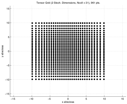
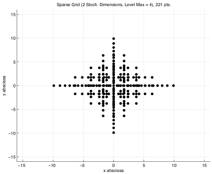
Figure 1: A Gauss-Hermite tensor-product grid (left) versus a Gauss-Hermite sparse grid (right) with a comparable number of points on each axis.

4.2 Collocation on sparse grids

In sparse grid collocation [56, 45], the polynomial accuracy is prescribed in terms of total degree. Sparse grids rules require much fewer points than tensor product rules as the dimension increases, but have the same asymptotic accuracy. This makes them applicable for problems with high number of stochastic dimensions. A tensor grid and a sparse grid rules that are comparable in terms of accuracy are shown in Figure 1.

Sparse grid rules are constructed hierarchically as linear combination of tensor products of nested one-dimensional rules, so that the total polynomial degree is a constant independent of dimension. The $N_{\textrm{term}}$-dimensional sparse grid quadrature rule of level $\ell_{\textrm{max}}$ is accurate to degree $(2\cdot\ell_{\textrm{max}}+1)$.

Each level between $\ell_{\textrm{max}}$ and $\ell_{\textrm{min}}=\max\{0,\ell_{\textrm{max}}-N_{\textrm{term}}+1\}$ is associated with a multi-index $\mathbf{p}=(p_{1},\ldots,p_{N_{\textrm{term}}})$, where $|\mathbf{p}|=\sum p_{i}$ denotes the levels of one dimensional rules used in each stochastic dimension. We consider the Gauss-Hermite points $\mathcal{H}(2^{p_{i}+1}-1)$ as the one dimensional abscissae of level $p_{i}$. Level $0$ consists of a single point, and for every subsequent level the number of points doubles plus one. For each partition $\mathbf{p}$, let the multi-index $\mathbf{m}=2^{\mathbf{p}+\mathbf{1}}-\mathbf{1}$ denote its degree. The $N_{\textrm{term}}$-dimensional sparse grid Gauss-Hermite interpolant is given by

$$\mathcal{I}^{\textrm{SG}}_{\ell_{\textrm{max}}}f(\mathbf{y})=\sum_{\ell_{\textrm{min}}\leq|\mathbf{p}|\leq\ell_{\textrm{max}}}(-1)^{\ell_{\textrm{max}}-|\mathbf{p}|}\cdot\binom{N_{\textrm{term}}-1}{\ell_{\textrm{max}}-|\mathbf{p}|}\cdot\mathcal{I}^{\textrm{TG}}_{\mathbf{m}}f(\mathbf{y}),$$

and the set of abscissae is

$$\mathcal{S}(\ell_{\textrm{min}},\ell_{\textrm{max}},N_{\textrm{term}})=\bigcup_{\ell_{\textrm{min}}\leq|\mathbf{p}|\leq\ell_{\textrm{max}}}\bigotimes_{i=1}^{N_{\textrm{term}}}\mathcal{H}(2^{p_{i}+1}-1).$$

5 Collocation-MMMFEM algorithms for Stokes-Darcy

As noted above, computing the fully discrete approximation to (16)–(18) in the coupled physical-stochastic space requires solving a sequence of deterministic Stokes-Darcy problems (24)–(26). These are solved in parallel by using a non-overlapping domain decomposition algorithm developed in [53]. It reduces to global fine scale problem to a coarse scale symmetric and positive definite interface problem, which is solved by a Krylov iterative solver such as the Conjugate Gradient (CG) method. We develop three algorithms that combine different implementations of the domain decomposition algorithm with stochastic collocation. The first method is based on the traditional domain decomposition algorithm, which requires solving subdomain problems at every CG iteration. The number of subdomain solves, which is the dominant cost in the algorithm, is proportional to the product of the total number of stochastic collocation points and the number of interface iterations. The other two methods exploit the efficiency of precomputing a multiscale flux basis, which is used to replace the subdomain solves by linear combination of the basis functions. One of these methods, referred to as deterministic multiscale flux basis, computes a new multiscale basis at each stochastic collocation. The number of subdomain solves for this method is proportional to the product of the total number of stochastic collocation points and the number of mortar degrees of freedom per subdomain. For the last method we follow the approach in [35] to gain additional efficiency by exploding the locality of the KL expansions. In particular, we precompute a full multiscale flux basis on each subdomain for all local stochastic realizations before the global collocation loop begins. This stochastic basis is reused multiple times during the global collocation loop, since the same local subdomain stochastic realization occurs over multiple global realizations. In this method, referred to as stochastic multiscale flux basis, the number of subdomain solves is proportional to the product of the number of mortar degrees of freedom per subdomain and the number of local stochastic collocation points, resulting in additional computational savings.

5.1 Reduction to an interface problem

Before presenting the three algorithms, we describe the non-overlapping domain decomposition algorithm for solving the deterministic Stokes-Darcy problem (24)–(26) that reduces the global problem to a coarse scale interface problem. We split (24)–(26) into two sets of complementary subproblems, one with specified interface data and all other data set to zero, and the other with zero interface data and the given source term and outside boundary conditions. For Stokes subdomains $D_{i}$, $1\leq i\leq N_{s}$, one of the subproblems is to find $\mathbf{u}_{h,i}^{*,\{k\}}({\boldsymbol{\lambda}})\in\widetilde{V}_{h,i}/\ker\,\tilde{a}_{i}$ and $p_{h,i}^{*,\{k\}}({\boldsymbol{\lambda}})\in\widetilde{W}_{h,i}$ with specified ${\boldsymbol{\lambda}}=(\lambda_{n},{\boldsymbol{\lambda}}_{\tau})$, where $\lambda_{n}$ and ${\boldsymbol{\lambda}}_{\tau}=(\lambda^{1}_{\tau},\ldots,\lambda^{d-1}_{\tau})$ represent the normal stress and tangential stress on $\Gamma_{ss}$, respectively, such that

$$\tilde{a}_{i}(\mathbf{u}_{h,i}^{*,\{k\}}({\boldsymbol{\lambda}}),\mathbf{v}_{i})+\tilde{b}_{i}(\mathbf{v}_{i},p_{h,i}^{*,\{k\}}({\boldsymbol{\lambda}}))$$

$$\qquad\qquad=-\langle\lambda_{n},\mathbf{v}_{i}\cdot\mathbf{n}_{i}\rangle_{\Gamma_{i}}-\sum_{l=1}^{d-1}\langle\lambda_{\tau}^{l},\mathbf{v}_{i}\cdot\mbox{\boldmath$\tau$}_{i}^{l}\rangle_{\Gamma_{i}\cap\Gamma_{ss}},\quad\forall\,\mathbf{v}_{i}\in\widetilde{V}_{h,i}/\ker\,\tilde{a}_{i},$$ (27)

$$\tilde{b}_{i}(\mathbf{u}_{h,i}^{*,\{k\}}({\boldsymbol{\lambda}}),w_{i})=0,\quad\forall\,w_{i}\in\widetilde{W}_{h,i},$$ (28)

where $\{\mbox{\boldmath$\tau$}_{i}^{l}\}_{l=1}^{d-1}$ is an orthogonal set of unit vectors tangential to $\partial D_{i}$ and the kernel space $\ker\,\tilde{a}_{i}:=\{\mathbf{v}\in\widetilde{V}_{i}:\tilde{a}_{i}(\mathbf{v},\mathbf{v})=0\}$ consists of a subset of all rigid body motions depending on the boundary types of $D_{i}$. For more detail we refer the reader to [53]. The complementary subproblem is to find $\bar{\mathbf{u}}^{\{k\}}_{h,i}\in\widetilde{V}_{h,i}/\ker\,a_{i}$ and $\bar{p}^{\{k\}}_{h,i}\in\widetilde{W}_{h,i}$ such that

$$\tilde{a}_{i}(\bar{\mathbf{u}}^{\{k\}}_{h,i},\mathbf{v}_{i})+\tilde{b}_{i}(\mathbf{v}_{i},\bar{p}^{\{k\}}_{h,i})=(\mathbf{f}_{i},\mathbf{v}_{i})_{D_{i}},\quad\forall\,\mathbf{v}_{i}\in\widetilde{V}_{h,i}/\ker\,a_{i},$$ (29)

$$\tilde{b}_{i}(\bar{\mathbf{u}}^{\{k\}}_{h,i},w_{i})=0,\quad\forall\,w_{i}\in\widetilde{W}_{h,i}.$$ (30)

Note that the first problem (27)–(28) has specified normal stress on the interface with zero boundary condition and source term, while the second problem (29)–(30) has specified boundary condition and source term and zero normal stress on the interface. Similarly, on the Darcy subdomains $D_{i}$, $N_{s}+1\leq i\leq N$, the first subproblem is to find $\mathbf{u}_{h,i}^{*,\{k\}}(\lambda)\in\widetilde{V}_{h,i}$ and $p_{h,i}^{*,\{k\}}(\lambda)\in\widetilde{W}_{h,i}$ with specified pressure $\lambda$ such that

$$\tilde{a}_{d,i}(\mathbf{u}_{h,i}^{*,\{k\}}(\lambda),\mathbf{v}_{i})+\tilde{b}_{i}(\mathbf{v}_{i},p_{h,i}^{*,\{k\}}(\lambda))=-\langle\lambda,\mathbf{v}_{i}\cdot\mathbf{n}_{i}\rangle_{\Gamma_{i}},\quad\forall\,\mathbf{v}_{i}\in\widetilde{V}_{h,i},$$ (31)

$$\tilde{b}_{i}(\mathbf{u}_{h,i}^{*,\{k\}}(\lambda),w_{i})=0,\quad\forall\,w_{i}\in\widetilde{W}_{h,i}.$$ (32)

The complementary subproblem is to find $\bar{\mathbf{u}}^{\{k\}}_{h,i}\in\widetilde{V}_{h,i}$ and $\bar{p}^{\{k\}}_{h,i}\in\widetilde{W}_{h,i}$ such that

$$\tilde{a}_{i}(\bar{\mathbf{u}}^{\{k\}}_{h,i},\mathbf{v}_{i})+\tilde{b}_{i}(\mathbf{v}_{i},\bar{p}^{\{k\}}_{h,i})=(\mathbf{f}_{i},\mathbf{v}_{i})_{D_{i}},\quad\forall\,\mathbf{v}_{i}\in\widetilde{V}_{h,i},$$ (33)

$$\tilde{b}_{i}(\bar{\mathbf{u}}^{\{k\}}_{h,i},w_{i})=-(q_{d},w_{i})_{D_{i}},\quad\forall\,w_{i}\in\widetilde{W}_{h,i}.$$ (34)

Using the interface condition (26), it is easy to see that (24)–(26) is equivalent to solving the interface problem: find $\lambda^{\{k\}}_{H}\in\widetilde{\Lambda}_{H}$ such that

$$s_{H}(\lambda^{\{k\}}_{H},\mu):=-\tilde{b}_{\Lambda}(\mathbf{u}^{*,\{k\}}_{h}(\lambda^{\{k\}}_{H}),\mu)=\tilde{b}_{\Lambda}(\bar{\mathbf{u}}^{\{k\}}_{h},\mu),\quad\forall\,\mu\in\widetilde{\Lambda}_{H},$$ (35)

and recovering the global velocity and pressure by

$$\mathbf{u}^{\{k\}}_{h}=\mathbf{u}^{*,\{k\}}_{h}(\lambda^{\{k\}}_{H})+\bar{\mathbf{u}}^{\{k\}}_{h},\quad p^{\{k\}}_{h}=p_{h}(\lambda^{\{k\}}_{H})+\bar{p}^{\{k\}}_{h}.$$

It is shown in [53] that the bilinear form $s_{H}(\cdot,\cdot)$ in (35) is symmetric and positive definite. We employ the CG method for its solution.

The interface problem (35) can be rewritten in an operator form

$$S_{H}^{\{k\}}\lambda_{H}^{\{k\}}=g_{H}^{\{k\}},$$ (36)

where $S_{H}^{\{k\}}:\widetilde{\Lambda}_{H}\rightarrow\widetilde{\Lambda}_{H}$ is a Steklov–Poincaré type operator, defined as

$$\left(S_{H}^{\{k\}}\lambda,\mu\right)=s_{H}^{\{k\}}(\lambda,\mu),\quad\forall\lambda,\mu\in\widetilde{\Lambda}_{H},$$

and $g_{H}^{\{k\}}$ is defined by $\langle g_{H}^{\{k\}},\mu\rangle_{\Gamma}=\tilde{b}_{\Lambda}(\bar{\mathbf{u}}_{h}^{\{k\}},\mu),\ \ \forall\mu\in\widetilde{\Lambda}_{H}$.

It is important to note that the dominant cost in solving (36) is computing the action of operator $S_{H}^{\{k\}}$ in every CG iteration. This action involves solving the Neumann-to-Dirichlet problem (27)–(28) in the Stokes subdomains, and the Dirichlet-to-Neumann problem (31)–(32) in the Darcy subdomains.

Let $\widetilde{\Lambda}_{H,i}$ be the restriction of $\widetilde{\Lambda}_{H}$ to $\Gamma_{i}$ and let $S_{H,i}^{\{k\}}$ be the restriction of $S_{H}^{\{k\}}$ to $\widetilde{\Lambda}_{H,i}$. The action of $S_{H}^{\{k\}}$ can be written as the sum of the actions of the local operators:

$$S_{H}^{\{k\}}\lambda_{H}=\sum_{i=1}^{N}S_{H,i}^{\{k\}}\lambda_{H,i}.$$

We proceed with the description of the three methods for solving (36).

5.2 Method S1: Collocation without multiscale flux basis

Method S1 (without multiscale flux basis) For $k=1,\ldots,N_{real}$, do  Step 1: Generate a permeability realization $K^{\{k\}}$ corresponding to the global collocation index $k$.  Step 2: Solve (36) using traditional MMMFEM for $\lambda_{H}^{\{k\}}$.  Step 3: Add the solution to the statistical moments with the collocation weight applied. End do

In any subdomain, Step 2 costs one set of subdomain solves in every CG iteration for applying $S_{H}^{\{k\}}$. Given a mortar function $\lambda_{H}$, the action of $S_{H,i}^{\{k\}}\lambda_{H,i}$ in subdomain $D_{i}$ includes:

1. Project $\lambda_{H,i}$ onto subdomain boundaries: $\lambda_{h,i}=\mathcal{L}_{h,i}\lambda_{H,i}$, where $\mathcal{L}_{h,i}$ is the $L^{2}$-projection operator onto the velocity space (for Stokes) or the normal trace of the velocity space (for Darcy) on $\Gamma_{i}$.

2. If $D_{i}$ is a Darcy subdomain, solve the subdomain problem (31)–(32) with Dirichlet data $\lambda_{h,i}$; If $D_{i}$ is a Stokes subdomain, solve the subdomain problem (27)–(28) with Neumann data $\lambda_{h,i}$.

3. Project the resulting flux in Darcy or velocity in Stokes back to the mortar space and compute the jump across the interfaces.

Let $N_{\textrm{iter}}(k)$ be the number of CG iterations for the $k$th stochastic realization. Then in any subdomain $D_{i}$ the leading term in the number of solves for method S1 is

$$N_{S1}:=\sum_{k=1}^{N_{\textrm{real}}}N_{\textrm{iter}}(k),$$ (37)

omitting the extra solves in the right hand side and solution recovery. The number of CG iterations depends on the condition number of the interface operator $S_{H}^{\{k\}}$, which grows with refining the grids or increasing the number of subdomains or permeability contrast [53], resulting in possibly large computational cost of Method S1.

5.3 Method S2: Collocation with deterministic multiscale flux basis

One way to reduce the cost of the MMMFEM for Stokes-Darcy flow is to employ a multiscale flux basis following the method introduced in [33]. When solving the deterministic problem $\eqref{operatorform}$, before the CG iteration starts, we compute on each subdomain the local solution for every mortar degree of freedom associated with the subdomain and store the results as a basis of flux responses in Darcy or velocity responses in Stokes. Then to evaluate the action of $S_{H}^{\{k\}}$ in every interface iteration, we simply use the linear combination of the basis instead of performing an extra subdomain solve. The algorithm for this method is as follows:

Method S2 (with deterministic multiscale flux basis) For $k=1,\ldots,N_{real}$, do  Step 1: Generate a permeability realization $K^{\{k\}}$ corresponding to the global collocation index $k$.  Step 2: On each $D_{i}$, compute and save the multiscale flux basis $\{\phi_{H,i}^{j,\{k\}}\}_{j=1}^{N_{\textrm{dof},i}}$  Step 3: Solve (36) for $\lambda_{H}^{\{k\}}$ using the MMMFEM with the computed basis.  Step 4: Add the solution to the statistical moments with the collocation weight applied. End do

In Step 2, where $N_{\textrm{dof},i}$ is the number of mortar degrees of freedom on $\Gamma_{i}$, we solve a subdomain problem for each mortar basis function. The mortar basis functions $\{\xi_{H,i}^{j}\}_{j=1}^{N_{\textrm{dof},i}}\subset\widetilde{\Lambda}_{H,i}$ are defined such that any $\lambda_{H,i}\in\widetilde{\Lambda}_{H,i}$ can be expressed uniquely by their linear combination:

$$\lambda_{H,i}=\sum_{j=1}^{N_{\textrm{dof},i}}c_{i}^{j}\xi_{H,i}^{j}.$$

For any $j=1\ldots N_{\textrm{dof},i}$, the multiscale flux basis is computed by

$$\phi_{H,i}^{j,\{k\}}=S_{H,i}^{\{k\}}\xi_{H,i}^{j}.$$

To evaluate $S_{H,i}^{\{k\}}\lambda_{H,i}$ in Step 3, we simply compute

$$S_{H,i}^{\{k\}}\lambda_{H,i}=\sum_{j=1}^{N_{\textrm{dof},i}}c_{i}^{j}\phi_{H,i}^{j,\{k\}}.$$

Since there are no solves inside the CG loop, the number of subdomain solves for Method S2 does not depend on the number of CG iterations. In any subdomain $D_{i}$, the number of subdomain solves for Method S2 has the leading term

$$N_{S2}:=N_{\textrm{dof},i}*N_{\textrm{real}}.$$ (38)

Unlike the cost of Method S1 (37), the dominant cost of Method S2 is independent of the condition number of the interface operator, which makes it less sensitive to $h$, $H$, and jumps in $K$. Comparing (38) to (37), we observe that in every stochastic realization, Method S2 costs less than Method S1 if the number of CG iterations $N_{\textrm{iter}}(k)$ is greater than the maximum number of mortar degrees of freedom per subdomain.

5.4 Method S3: Collocation with stochastic multiscale flux basis

The third method, which utilizes the approach from [35], is designed to achieve greater computational savings than Method S2 by exploiting the fact that the global KL expansion is a sum of local KL expansions. The main idea is to compute and store a multiscale flux basis for all local KL realizations before the global stochastic collocation loop. Since a local KL realization is repeated multiple times in the global KL collocation loop, the precomputed stochastic multiscale flux basis can be reused, resulting in further gain in computational efficiency. Below we present the algorithm for method S3.

Method S3 (with stochastic multiscale flux basis) For any Darcy subdomain $D_{i}$ that belongs to KL region $j$, set $N_{\textrm{real}}(j)$ to be the number of local KL realization; for any Stokes subdomain, $N_{\textrm{real}}(j)$ is set to 1. Pre-computation loop: stochastic multiscale basis For $k=1,\ldots,N_{\textrm{real}}(j)$, do  Step 1: Generate a permeability realization $K^{\{k\}}$ corresponding to the local collocation index $k$.  Step 2: Compute and save the multiscale flux basis under the current local index. End do Main loop: global stochastic collocation For $l=1,\ldots,N_{real}$, do  Step 3: Generate a permeability realization $K^{\{l\}}$ corresponding to the global collocation index $l$.  Step 4: Convert the global index to the subdomain’s local index $k$  Step 5: Solve (36) for $\lambda_{H}^{\{k\}}$ using the MMMFEM with the computed basis for local index $k$ in step 2.  Step 6: Add the solution to the statistical moments with collocation weight applied. End do

The algorithms for index conversion in Step 4 for tensor product grid and sparse grid are given in Algorithms 5 and 6 in [35], respectively. Notice that all subdomain solves in Method S3, except the extra two for RHS computation and solution recovery, are done in the pre-computation loop only. Therefore in subdomain $D_{i}$, the total number of solves has the leading term

$$N_{S3}:=N_{\textrm{dof},i}*N_{\textrm{real}}(j).$$ (39)

Compared to the leading term in $N_{S2}$ for method S2 (38), $N_{S3}$ is proportional to $N_{\textrm{real}}(j)$ instead of $N_{\textrm{real}}$. When there exists more than one KL region in the problem setting, in any KL region $j$ the number of local realizations $N_{\textrm{real}}(j)$ is less than the number of global realizations $N_{\textrm{real}}$, which makes Method S3 cost less in terms of subdomain solves than Method S2.

6 Numerical tests

In this section, three numerical examples are presented to test both tensor product and sparse grid collocations with Methods S1, S2 and S3. All three examples are motivated by coupled surface flow with groundwater flow with uncertain non-stationary heterogeneous permeability. The covariance function in KL region $D_{KL}^{(i)}$ is

$$C_{Y}^{(i)}(\mathbf{x},\overline{\mathbf{x}})=\left(\sigma_{Y}^{(i)}\right)^{2}\exp\left[-\frac{|x_{1}-\overline{x}_{1}|}{\eta_{1}^{(i)}}-\frac{|x_{2}-\overline{x}_{2}|}{\eta_{2}^{(i)}}\right],$$ (40)

where $\sigma_{Y}^{(i)}$ is the variance and $\eta_{j}^{(i)}$ is the correlation length in the $j$th physical dimension. The three examples are designed to test different levels of heterogeneity and uncertainty in terms of number of KL regions, correlation length, and variance. In addition, test case 2 illustrates the flexibility to use finer physical discretization grids in KL regions with smaller correlation lengths, and test case 3 presents an application to domains with irregular geometry.

For all tests, we use Taylor-Hood [51] triangular finite element in Stokes and the lowest order Raviart-Thomas [47] quadrilateral finite elements in Darcy for space discretization. All interfaces are discretized via discontinuous piecewise linear mortar finite elements. The methods are implemented in parallel for distributed memory computers using message passing interface (MPI). The numerical tests are run on a parallel cluster of Intel Xeon CPU E5-2650 v3 @ 2.30GHz processors with 192GB RAM, with each subdomain assigned to one core.

6.1 Test case 1

The first test case has a global domain $(0,1)\times(0,1.2)$, where $D_{d}=(0,1)\times(0,0.8)$ and $D_{s}=(0,1)\times(0.8,1.2)$. The problem is divided into 6 equal-size subdomains with two Stokes and four Darcy subdomains, see Figure 2 (left). The outside boundary conditions are given as follows: in Darcy, zero pressure is specified on the bottom edge, and no-flow condition on the left and right edges; in Stokes, velocity is specified on the left and top edges, with a parabolic inflow profile on the left and zero normal velocity and a linearly decreasing tangential slip on the top, while zero normal and tangential stresses are specified on the right edge.

The mean permeability is a given heterogeneous scalar field, which varies two orders of magnitude, see Figure 2 (right). There are two rectangular statistically independent KL regions in Darcy, defined as $(0,1)\times(0,0.4)$ and $(0,1)\times(0.4,0.8)$. In the tensor product grid collocation test we set $N_{\textrm{term}}(1)=2\times 1=2$ and $N_{\textrm{term}}(2)=3\times 3=9$. In the sparse grid test we set $N_{\textrm{term}}(1)=N_{\textrm{term}}(2)=5\times 5=25$. In both KL regions we set $\sigma_{Y}^{(i)}=1.0$ and $\eta_{j}^{(i)}=0.1$. In tensor product collocation, the grid is isotropic with $N_{\textrm{coll}}=2$ in each stochastic dimension. In sparse grid collocation, $\ell_{\textrm{max}}=1$, so on both cases we have a third degree of accuracy in each stochastic dimension. For the tensor product grid, the number of terms in the global KL expansion is $N_{\textrm{term}}=2+9=11$, resulting in number of global realizations $N_{\textrm{real}}=N_{\textrm{coll}}^{N_{\textrm{term}}}=2^{11}=2048$. For the sparse grid, the number of terms in the global KL expansion is $N_{\textrm{term}}=25+25=50$, resulting in number of global realizations $N_{\textrm{real}}=2*N_{\textrm{term}}+1=101$.

For the physical space discretization, we have a local mesh of size $64\times 64$ in every Darcy subdomain and size $32\times 32$ in every Stokes subdomain. The mortar mesh is $8\times 1$ on every interface on $\Gamma_{dd}$ and $4\times 1$ on every interface on $\Gamma_{sd}\cup\Gamma_{ss}$. One realization of the computed velocity field is shown in Figure 2 left. We observe infiltration from the Stokes region into the Darcy region with higher velocity in the areas of higher permeability. The normal velocity across the Stokes-Darcy interface is continuous and reasonable well resolved, even with the fairly coarse mortar mesh. The tangential velocity along the Stokes-Darcy interface is higher in the Stokes region.

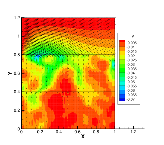
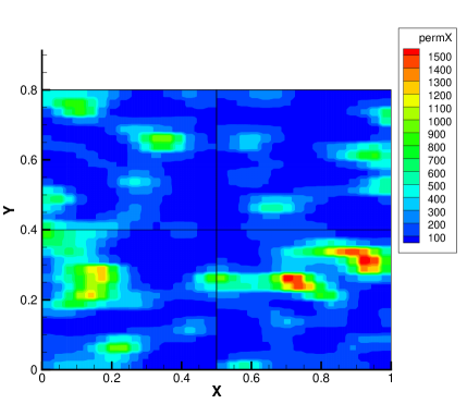
Figure 2: Case 1, solution realization - colors for vertical velocity and arrows for velocity vector (left) and permeability realization (right).

Tensor Product Collocation, $N_{\textrm{term}}=11$, $N_{\textrm{coll}}=2$ (2048 realizations)

	Method S1	Method S2	Method S3
Max. number of solves	1,499,257	167,936	45,056
Runtime in seconds	33457.4	4464.9	3357.1

Sparse Grid Collocation, $N_{\textrm{term}}=50$, $\ell_{\textrm{max}}=1$ (101 realizations)

	Method S1	Method S2	Method S3
Max. number of solves	71,237	8,282	4,282
Runtime in seconds	1566.1	220.5	156.8

Table 1: Number of subdomain solves and runtime in seconds for Case 1.

The number of solves and runtimes for all three methods on tensor product and sparse grid collocations are shown in Table 1. With tensor product collocation, Method S1 requires 1.5 million number of solves. Recalling (37), this very high number is due to the high value of $N_{\textrm{real}}=2048$, as well as a large number of CG iterations $N_{\textrm{iter}}(k)$ in each realization. In comparison, Methods S2 requires only about 11% of the number of solves and about 13% of the runtime of Method S1. We observe even larger savings in Method S3, which requires only about 27% of the number of solves of Method S2. This is due the fact that the stochastic multiscale basis in Method S3 is reused multiple times. In particular, recalling the leading costs (38) and (39), we note that $N_{\textrm{real}}=2^{11}$ and $N_{\textrm{real}}(2)=2^{9}$, resulting in a global to local ratio $N_{\textrm{real}}/N_{\textrm{real}}(2)=4.0$. However, the reduction in runtime in Method S3 compared to Method S2 is less significant, due to the additional cost of inter-processor communication at each CG iteration. Similar conclusions can be made in the sparse grid collocation case, where Method S2 requires about 12% of the subdomain solves and about 14% of the runtime of Method S1. Comparing Method S2 and Method S3, we note that Method S3 requires about 52% of the subdomain solves of Method S2, which is consistent with the global to local ratio $N_{\textrm{real}}/N_{\textrm{real}}(j)=101/51=1.99$. We conclude that higher global to local ratio results in increased reuse of the stochastic basis and increased reduction in the number of subdomain solves.

6.2 Test case 2

In this example we test a porous medium with an inclusion of higher and more heterogeneous permeability. The global domain $(0,1)^{2}$ is divided in half with the Stokes region on the top and the Darcy region on the bottom, and is partitioned into 32 subdomains. The outside boundary conditions are as in Case 1, with the exception that the zero normal velocity on the top edge is replaced with zero normal stress.

As shown in Figure 3, an L-shaped KL region 1 (red part) is contained within the Darcy domain, with its complement defined to be KL region 2 (gray part). In KL region 1, the mean permeability value is $e$, $\sigma_{Y}^{(1)}=1.0$ and $\eta_{j}^{(1)}=0.01$. In KL region 2, the mean permeability value is $e^{-1}$, $\sigma_{Y}^{(2)}=1.0$, and $\eta_{j}^{(2)}=0.1$. Note that in the inclusion, the mean permeability is more than 7 times larger and the correlation lengths are 10 times smaller than in the rest of the Darcy domain, see also the permeability realizations in top left panels in Figures 4 and 5. For the tensor product collocation, the grid is isotropic with $N_{\textrm{coll}}=2$ and $N_{\textrm{term}}=11$, where $N_{\textrm{term}}(1)=3\times 3$ and $N_{\textrm{term}}(2)=2\times 1$. For the sparse grid, we have $\ell_{\textrm{max}}=1$ and $N_{\textrm{term}}=200$, where $N_{\textrm{term}}(1)=14\times 14$ and $N_{\textrm{term}}(2)=2\times 2$. We note that in both collocation methods the number of KL terms is higher in the more heterogeneous L-shaped inclusion. Furthermore, with 196 KL terms for the sparse grid, the inclusion permeability is much more heterogeneous compared to the tensor product grid. The number of global realizations is $N_{\textrm{real}}=2^{11}=2048$ for tensor product and $N_{\textrm{real}}=2*200+1=401$ for sparse grid.

The physical space discretization is set as follows: for tensor product grid, we use a local mesh of $25\times 25$ in every Darcy subdomain and $8\times 8$ in every Stokes subdomain. A mortar mesh of $10\times 1$ is used on every interface on $\Gamma_{dd}$ and $4\times 1$ on every interface on $\Gamma_{sd}\cup\Gamma_{ss}$; for sparse grid, we use a local mesh of $20\times 20$ in every subdomain in the inclusion and $4\times 4$ elsewhere. A mortar mesh of $10\times 1$ is used on every interior interface of the inclusion, $4\times 1$ on each of its outside boundaries, and $2\times 1$ elsewhere.

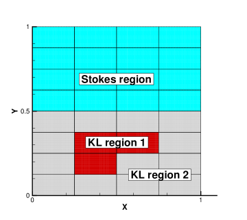
Figure 3: Case 2, illustration of KL regions.

Computed realizations, mean, and variance of the solution are shown in Figures 4 and 5 for tensor product and sparse grid, respectively. The general behavior of the flow is similar to Case 1, with a channel-like flow in the Stokes region infiltrating downward into the Darcy region. The largest vertical velocity is in the high permeability L-shaped inclusion. The computed solution variance indicates that the largest uncertainty in the velocity is within the inclusion, while the largest pressure uncertainty is along the Stokes-Darcy interface. As expected, the solution uncertainty is higher in the Darcy region, since there is no stochastic parameter in the Stokes region. Nevertheless, the solution uncertainty extends well into the Stokes region, being highest along the Stokes-Darcy interface. This is due to the fact that the coupling conditions imply that the solution is stochastic in the entire Stokes-Darcy domain.

The maximum number of subdomain solves and runtimes for Case 2 are shown in Table 2. We note that in the multiscale flux basis Methods S2 and S3, the subdomain with the maximum number of solves is the one at the corner of L-shaped region, since it has the highest number of mortar degrees of freedom on its interfaces. For the tensor product grid, Method S2 requires only 11% of the subdomain solves in Method S1 and 52% of the runtime. These numbers for the sparse grid are 13% and 83%, respectively. Again, the smaller gain in runtime is due to the inter-processor communication overhead, which is even more significant in the example because of the larger number of subdomains. As in Case 1, the stochastic multiscale basis Method S3 results in additional computational gain compared to Method S2. For tensor product grid Method S3 requires 26% of the subdomain solves of Method S2, which is consistent with the global to local ratio $N_{\textrm{real}}/N_{\textrm{real}}(1)=2^{11}/2^{9}=4.0$. However, the gain with sparse grid is much smaller, with Method S3 requiring 98% of the maximum number of subdomain solves of Method S2. This again can be explained with the global to local ratio. In particular, $N_{\textrm{real}}/N_{\textrm{real}}(1)=401/193=1.02$, thus the stochastic basis in KL region 1 is reused very few times. Such situation occurs when most of the dimensions in the global stochastic space are contained within one KL region, as is the case here, with 196 KL terms in KL region 1 out of total of 200 KL terms.

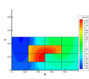
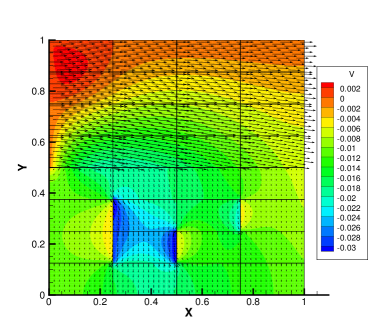
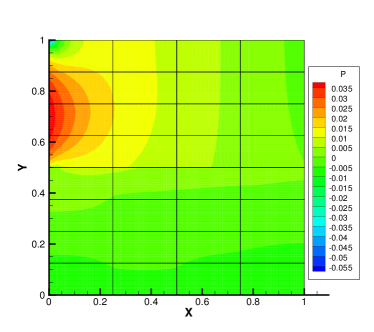
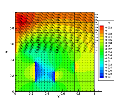
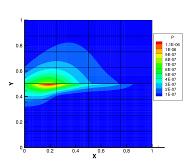
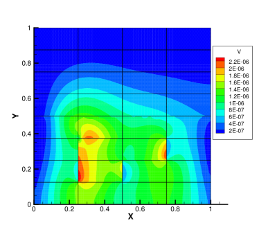
Figure 4: Case 2, tensor product grid, permeability realization (top-left), velocity realization (top-right), pressure mean value (middle-left), velocity mean value (middle-right), pressure variance (bottom-left), vertical velocity variance of (bottom-right).

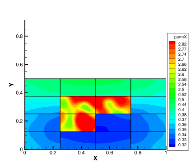
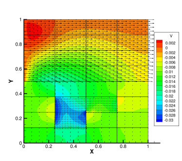
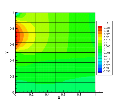
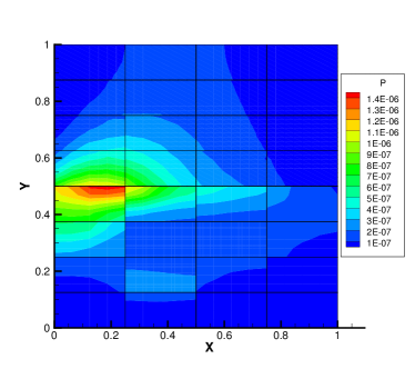
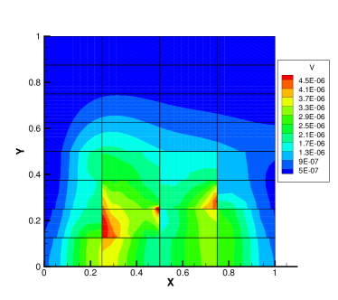
Figure 5: Case 2, sparse grid, permeability realization (top-left), velocity realization (top-right), pressure mean value (middle-left), velocity mean value (middle-right), pressure variance (bottom-left), vertical velocity variance of (bottom-right).

Tensor Product Collocation, $N_{\textrm{term}}=11$, $N_{\textrm{coll}}=2$ (2048 realizations) Method S1 Method S2 Method S3 Max. number of solves 3,033,494 331,776 86,016 Runtime in seconds 5893.3 3155.9 2707.6

Sparse Grid Collocation, $N_{\textrm{term}}=200$, $\ell_{\textrm{max}}=1$ (401 realizations) Method S1 Method S2 Method S3 Max. number of solves 346,709 45,714 44,818 Runtime in seconds 525.5 435.1 391.2

Table 2: Number of subdomain solves and runtime in seconds for Case 2.

6.3 Test case 3

The third test is a coupled surface water and groundwater flow with realistic geometry and highly heterogeneous permeability. The computational domain is shown in Figure 6 (right). There are $4\times 2=8$ subdomains on the global irregular region with Stokes in the top half and Darcy on the bottom. The outside boundary conditions are given as follows: in Darcy, zero pressure is specified on the bottom, and no-flow on left and right; for the Stokes region, inflow velocity is specified on the left and zero velocity on the right, along with zero normal and tangential stresses on the top. The mean permeability over the entire Darcy region is generated by a single realization of a global KL expansion truncated after 400 terms, with mean value one and covariance given in (40) with variance $\sigma_{Y}=2.1$ and correlation lengths $\eta_{1}=0.1$ and $\eta_{2}=0.05$. There are four KL regions in Darcy, represented by each one of the four Darcy subdomains, as shown in Figure 6 (top-left). In all KL regions, the variance is $\sigma_{Y}^{(i)}=1.0$ and the correlation lengths are $\eta_{j}^{(i)}=0.1$. One realization of the permeability field with tensor product collocation is presented in Figure 6 (bottom-left). For tensor product collocation, the grid is isotropic with $N_{\textrm{coll}}=2$, the stochastic dimensions are set by $N_{\textrm{term}}(j)=2\times 1$ for $j=1,2,3,4$ and $N_{\textrm{term}}=8$ in total. For sparse grid collocation, we have $\ell_{\textrm{max}}=1$ and $N_{\textrm{term}}=100$ with $N_{\textrm{term}}(j)=5\times 5$ for $j=1,2,3,4$. The physical grids are alternating $18\times 15$ and $15\times 12$ in the Darcy subdomains, and $12\times 15$ and $9\times 12$ in the Stokes subdomains. Mortar meshes of $4\times 1$ are used on all interfaces.

To handle the irregular geometry, we employ the multipoint flux mixed finite element method on quadrilaterals in the Darcy region [54], which can be reduced to a cell-centered finite difference scheme for the pressure. We impose the mortar conditions on curved interfaces by mapping the physical grids to reference grids with flat interfaces. For more details about this implementation, the reader is referred to [50].

Figure 7 shows the mean and variance of the computed solution with tensor product grid (left) and sparse grid (right). The predicted mean velocity with the two methods is similar, indicating that it is well resolved with both stochastic collocation methods. The computed variance is larger and better resolved with the sparse grid, due to the larger number of KL terms.

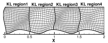
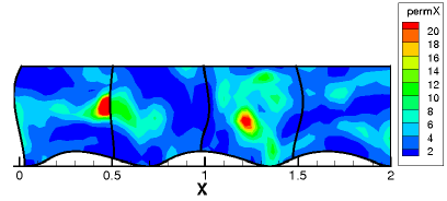
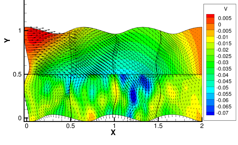
Figure 6: Case 3, KL regions and meshes (top-left), permeability realization (bottom-left), velocity realization (right).

Tensor Product Collocation, $N_{\textrm{term}}=8$, $N_{\textrm{coll}}=2$ (256 realizations) Method S1 Method S2 Method S3 Max. number of solves 58,728 21,248 960 Runtime in seconds 255.5 192.8 91.7

Sparse Grid Collocation, $N_{\textrm{term}}=100$, $\ell_{\textrm{max}}=1$ (201 realizations) Method S1 Method S2 Method S3 Max. number of solves 45,031 16,683 3,051 Runtime in seconds 178.3 107.4 82.6

Table 3: Number of subdomain solves and runtime in seconds for Case 3.

            

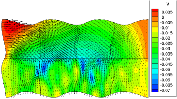
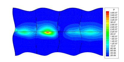
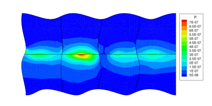
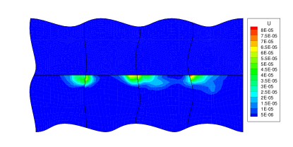
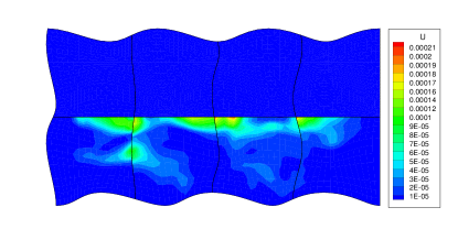
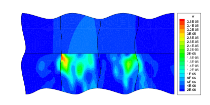
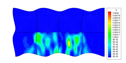
Figure 7: Case 3, solution with tensor product grid (left) and sparse grid (right); from top to bottom: velocity mean, pressure variance, horizontal velocity variance, vertical velocity variance.

The computational cost for Case 3 is presented in Table 3. The number of global stochastic realizations is $N_{\textrm{real}}=256$ in tensor product and $N_{\textrm{real}}=201$ in sparse grid. The number of subdomain solves for Method S1 is smaller compared to the previous examples, due to the fewer realizations and fewer CG iterations. Thus smaller computational savings with Methods S2 and S3 are expected. Nevertheless, with tensor product grid, Method S2 requires 36% of the subdomain solves of Method S1 and 75% of the runtime. With sparse grid, it requires 37% of the solves of Method S1 and 60% of the runtime. The global to local ratio in this case is larger, $N_{\textrm{real}}/N_{\textrm{real}}(j)=256/4=64$ for tensor product grid and $N_{\textrm{real}}/N_{\textrm{real}}(j)=201:51=3.94$ for sparse grid. This results in significant savings in Method S3 compared with Method S2 in terms of subdomain solves, with Method S3 requiring only 4.5% of the solves and 48% of the runtime with tensor product grid, and 18% of the solves and 77% of the runtime with sparse grid.

7 Conclusions

We have presented three algorithms for solving the coupled stochastic Stokes-Darcy problem with non-stationary porous media, one of which does not use a multiscale flux basis and the other two use deterministic and stochastic multiscale flux basis, respectively. The discretization includes stochastic collocation methods in the stochastic space and the MMMFEM in the physical space. The numerical tests in Section 6 demonstrate that the proposed algorithms can compute accurate statistical moments of the solution for a wide range of permeability heterogeneity and uncertainty, number of KL regions and KL terms. We generally observe a significant reduction in the number of subdomain solves when the multiscale flux basis is utilized for solving the coarse-scale mortar interface problem. The stochastic multiscale flux basis results in significant additional savings, due to its reuse during the global collocation loop, especially in the cases with large global to local realizations ratio, such as using tensor product grid collocation or having more KL regions. In all algorithms, the inter-processor communication cost in each CG iteration becomes a factor when the local problems are relatively cheap. A balancing preconditioner for the Darcy region [44, 46] could be used to reduce the number of iterations. A possible extension of this work is to incorporate stochasticity in the source term of the Stokes equation, e.g., in modeling rainfall in surface-subsurface flow simulations. In that case, one would expect even larger computational savings from the use of the stochastic multiscale flux basis.

References

- [1] J. Aarnes and Y. Efendiev. Mixed multiscale finite element methods for stochastic porous media flows. SIAM J. Sci. Comput., 30(5):2319–2339, 2008.
- [2] J. Aarnes, S. Krogstad, and K.-A. Lie. A hierarchical multiscale method for two-phase flow based upon mixed finite elements and nonuniform coarse grids. Multiscale Model. Simul., 5(2):337–363, 2006.
- [3] T. Arbogast. Implementation of a locally conservative numerical subgrid upscaling scheme for two-phase Darcy flow. Comput. Geosci., 6(3-4):453–481, 2002. Locally conservative numerical methods for flow in porous media.
- [4] T. Arbogast. Analysis of a two-scale, locally conservative subgrid upscaling for elliptic problems. SIAM J. Numer. Anal., 42:576–598, 2004.
- [5] T. Arbogast, G. Pencheva, M. Wheeler, and I. Yotov. A Multiscale Mortar Mixed Finite Element Method. Multiscale Model. Simul., 6(1):319, 2007.
- [6] D. N. Arnold, F. Brezzi, and M. Fortin. A stable finite element for the Stokes equations. Calcolo, 21(4):337–344 (1985), 1984.
- [7] B. Asokan and N. Zabaras. A stochastic variational multiscale method for diffusion in heterogeneous random media. J. Comp. Physics, 218(2):654–676, 2006.
- [8] I. Babuška, F. Nobile, and R. Tempone. A stochastic collocation method for elliptic partial differential equations with random input data. SIAM J. Numer. Anal., 45(3):1005–1034, 2008.
- [9] G. Beavers and D. Joseph. Boundary conditions at a naturally impermeable wall. J. Fluid. Mech, 30:197–207, 1967.
- [10] F. Brezzi, J. Douglas, Jr., and L. D. Marini. Two families of mixed elements for second order elliptic problems. Numer. Math., 88:217–235, 1985.
- [11] H. Chang and D. Zhang. A comparative study of stochastic collocation methods for flow in spatially correlated random fields. Commun. Comput. Phys., 6(3):509–535, 2009.
- [12] J. Chen, S. Sun, and X.-P. Wang. A numerical method for a model of two-phase flow in a coupled free flow and porous media system. J. Comput. Phys., 268:1–16, 2014.
- [13] W. Chen, D. Han, and X. Wang. Uniquely solvable and energy stable decoupled numerical schemes for the Cahn-Hilliard-Stokes-Darcy system for two-phase flows in karstic geometry. Numer. Math., 137(1):229–255, 2017.
- [14] Z. Chen and T. Hou. A mixed multiscale finite element method for elliptic problems with oscillating coefficients. Math. Comp., 72:541–576, 2003.
- [15] E. Chung, Y. Efendiev, and T. Y. Hou. Adaptive multiscale model reduction with generalized multiscale finite element methods. J. Comput. Phys., 320(C):69–95, Sept. 2016.
- [16] E. Chung, Y. Efendiev, and C. Lee. Mixed generalized multiscale finite element methods and applications. Multiscale Model. Simul., 13(1):338–366, 2015.
- [17] M. Crouzeix and P.-A. Raviart. Conforming and nonconforming finite element methods for solving the stationary Stokes equations. I. Rev. Française Automat. Informat. Recherche Opérationnelle Sér. Rouge, 7(R-3):33–75, 1973.
- [18] C. Dawson. A continuous/discontinuous Galerkin framework for modeling coupled subsurface and surface water flow. Comput. Geosci., 12(4):451–472, 2008.
- [19] M. Deb, I. Babuška, and J. Oden. Solution of stochastic partial differential equations using Galerkin finite element techniques. Comput. Methods Appl. Mech. Eng., 190(48):6359–6372, 2001.
- [20] M. Discacciati, E. Miglio, and A. Quarteroni. Mathematical and numerical models for coupling surface and groundwater flows. Appl. Numer. Math., 43(1-2):57–74, 2002. 19th Dundee Biennial Conference on Numerical Analysis (2001).
- [21] M. Discacciati and A. Quarteroni. Analysis of a domain decomposition method for the coupling of Stokes and Darcy equations. In Numerical mathematics and advanced applications, pages 3–20. Springer Italia, Milan, 2003.
- [22] M. Discacciati and A. Quarteroni. Convergence analysis of a subdomain iterative method for the finite element approximation of the coupling of Stokes and Darcy equations. Comput. Vis. Sci., 6(2-3):93–103, 2004.
- [23] P. Dostert, Y. Efendiev, and T. Hou. Multiscale finite element methods for stochastic porous media flow equations and application to uncertainty quantification. Comput. Methods Appl. Mech. Eng., 197(43-44):3445–3455, 2008.
- [24] Y. Efendiev, J. Galvis, and T. Y. Hou. Generalized multiscale finite element methods (GMsFEM). J. Comp. Physics, 251:116 – 135, 2013.
- [25] C. Farhat and F. Roux. A method of finite element tearing and interconnecting and its parallel solution algorithm. Internat. J. Methods Engrg., 32:1205–1227, 1991.
- [26] G. Fishman. Monte Carlo: Concepts, Algorithms, and Applications. Springer, Berlin, 1996.
- [27] J. Galvis and Y. Efendiev. Domain decomposition preconditioners for multiscale flows in high-contrast media. Multiscale Model. Simul., 8(4):1461–1483, 2010.
- [28] J. Galvis and M. Sarkis. Non-matching mortar discretization analysis for the coupling Stokes-Darcy equations. Electron. Trans. Numer. Anal., 26:350–384, 2007.
- [29] J. Galvis and M. Sarkis. FETI and BDD preconditioners for Stokes-Mortar-Darcy systems. Commun. Appl. Math. Comput. Sci., 5:1–30, 2010.
- [30] B. Ganapathysubramanian and N. Zabaras. Modelling diffusion in random heterogeneous media: Data-driven models, stochastic collocation and the variational multi-scale method. J. Comp. Physics, 226:326–353, 2007.
- [31] B. Ganis, H. Klie, M. Wheeler, T. Wildey, I. Yotov, and D. Zhang. Stochastic collocation and mixed finite elements for flow in porous media. Comput. Methods Appl. Mech. Eng., 197(43-44):3547–3559, 2008.
- [32] B. Ganis, G. Pencheva, M. F. Wheeler, T. Wildey, and I. Yotov. A frozen Jacobian multiscale mortar preconditioner for nonlinear interface operators. Multiscale Model. Simul., 10(3):853–873, 2012.
- [33] B. Ganis, D. Vassilev, C. Wang, and I. Yotov. A multiscale flux basis for mortar mixed discretizations of Stokes-Darcy flows. Comput. Methods Appl. Mech. Engrg., 313:259–278, 2017.
- [34] B. Ganis and I. Yotov. Implementation of a Mortar Mixed Finite Element Method using a Multiscale Flux Basis. Comput. Methods Appl. Mech. Eng., 198(49-52):3989–3998, 2009.
- [35] B. Ganis, I. Yotov, and M. Zhong. A stochastic mortar mixed finite element method for flow in porous media with multiple rock types. SIAM Journal on Scientific Computing, 33(3):1439–1474, 2011.
- [36] R. Ghanem and P. Spanos. Stochastic Finite Elements: A Spectral Approach. Springer-Verlag, New York, 1991.
- [37] V. Girault, D. Vassilev, and I. Yotov. Mortar multiscale finite element methods for Stokes-Darcy flows. Numerische Mathematik, 127:93–165, 2014.
- [38] R. Glowinski and M. Wheeler. Domain decomposition and mixed finite element methods for elliptic problems. In First International Symposium on Domain Decomposition Methods for Partial Differential Equations, Philadelphia, PA, 1988.
- [39] R. H. W. Hoppe, P. Porta, and Y. Vassilevski. Computational issues related to iterative coupling of subsurface and channel flows. Calcolo, 44(1):1–20, 2007.
- [40] T. Hou and X. Wu. A multiscale finite element method for elliptic problems in composite materials and porous media. J. Comp. Physics, 134(1):169–189, 1997.
- [41] T. Hughes, G. Feijóo, L. Mazzei, and J. Quincy. The variational multiscale method: a paradigm for computational mechanics. Comput. Methods Appl. Mech. Eng., 166(1-2):3–24, 1998.
- [42] W. Layton, F. Schieweck, and I. Yotov. Coupling fluid flow with porous media flow. SIAM J. Numer. Anal., 40(6):2195–2218, 2003.
- [43] Z. Lu and D. Zhang. Stochastic simulations for flow in nonstationary randomly heterogeneous porous media using a KL-based moment-equation approach. Multiscale Model. Simul., 6(1):228–245, 2008.
- [44] J. Mandel. Balancing domain decomposition. Communications in Numerical Methods for Engineering, 9(3):233–241, 1993.
- [45] F. Nobile, R. Tempone, and C. Webster. A sparse grid stochastic collocation method for partial differential equations with random input data. SIAM J. Numer. Anal., 46(5):2309–2345, 2008.
- [46] G. Pencheva and I. Yotov. Balancing domain decomposition for mortar mixed finite element methods on non-matching grids. Numer. Linear Algebra Appl., 10:159–180, 2003.
- [47] R. A. Raviart and J. M. Thomas. A mixed finite element method for 2nd order elliptic problems. In Mathematical Aspects of the Finite Element Method, Lecture Notes in Mathematics, volume 606, pages 292–315. Springer-Verlag, New York, 1977.
- [48] B. Rivière and I. Yotov. Locally conservative coupling of Stokes and Darcy flows. SIAM J. Numer. Anal., 42(5):1959–1977, 2005.
- [49] P. Saffman. On the boundary condition at the surface of a porous media. Stud. Appl. Math., L, (2):93–101, 1971.
- [50] P. Song, C. Wang, and I. Yotov. Domain decomposition for Stokes-Darcy flows with curved interfaces. Procedia Computer Science, 18:1077–1086, 2013.
- [51] C. Taylor and P. Hood. A numerical solution of the Navier-Stokes equations using the finite element technique. Internat. J. Comput. & Fluids, 1(1):73–100, 1973.
- [52] A. Toselli and O. Widlund. Domain Decomposition Methods - Algorithms and Theory. Springer-Verlag Berlin Heidelberg, 2005.
- [53] D. Vassilev, C. Wang, and I. Yotov. Domain decomposition for coupled Stokes and Darcy flows. Comput. Methods Appl. Mech. Engrg., 268:264–283, 2014.
- [54] M. F. Wheeler, G. Xue, and I. Yotov. A multiscale mortar multipoint flux mixed finite element method. ESAIM: Mathematical Modelling and Numerical Analysis (M2AN), 46(4):759–796, 2012.
- [55] C. L. Winter and D. M. Tartakovsky. Groundwater flow in heterogeneous composite aquifers. Water Resour. Res., 38(8), 2002.
- [56] D. Xiu and J. Hesthaven. High-order collocation methods for differential equations with random inputs. SIAM J. Sci. Comput., 27(3):1118–1139, 2005.
- [57] D. Xiu and G. Karniadakis. Modeling uncertainty in steady state diffusion problem via generalized polynomial chaos. Comput. Methods Appl. Mech. Eng., 191:4927–4948, 2002.
- [58] D. Zhang. Stochastic Methods for Flow in Porous Media: Coping with Uncertainties. Academic Press, San Diego, Calif., 2002.
- [59] D. Zhang and Z. Lu. An efficient, high-order perturbation approach for flow in random porous media via Karhunen–Loève and polynomial expansions. J. Comp. Physics, 194(2):773–794, 2004.