REGAL: Representation Learning-based Graph Alignment

Abstract.

Problems involving multiple networks are prevalent in many scientific and other domains. In particular, network alignment, or the task of identifying corresponding nodes in different networks, has applications across the social and natural sciences. Motivated by recent advancements in node representation learning for single-graph tasks, we propose REGAL (REpresentation learning-based Graph ALignment), a framework that leverages the power of automatically-learned node representations to match nodes across different graphs. Within REGAL we devise xNetMF, an elegant and principled node embedding formulation that uniquely generalizes to multi-network problems. Our results demonstrate the utility and promise of unsupervised representation learning-based network alignment in terms of both speed and accuracy. REGAL runs up to $30\times$ faster in the representation learning stage than comparable methods, outperforms existing network alignment methods by 20 to 30% accuracy on average, and scales to networks with millions of nodes each.

1. Introduction

Networks are powerful structures that naturally capture the wealth of relationships in our interconnected world, such as co-authorships, email exchanges, and friendships (Koutra and Faloutsos, 2017). The data mining community has accordingly proposed various methods for numerous tasks over a single network, like anomaly detection, link prediction, and user modeling. However, many graph mining tasks involve joint analysis of nodes across multiple networks. Some problems, like network alignment (Bayati et al., 2013; Zhang and Tong, 2016; Koutra et al., 2013a) and graph similarity (Koutra et al., 2013b), are inherently defined in terms of multiple graphs. In other cases, it is desirable to perform analysis across a collection of graphs, such as the MRI-based brain graphs of patients (Fallani et al., 2014), or snapshots of a temporal graph (Shah et al., 2015).

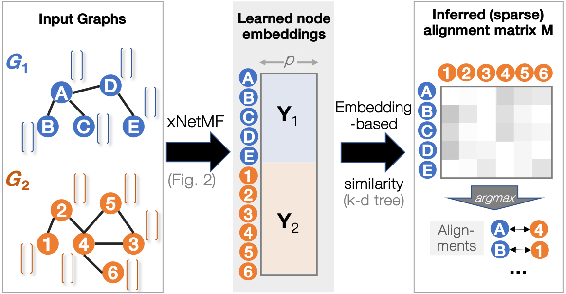
Figure 1. Pipeline of proposed graph alignment method, REGAL, based on our xNetMF representation learning method.

In this work, we study network alignment or matching, which is the problem of finding corresponding nodes in different networks. Network alignment is crucial for identifying similar users in different social networks, analyzing chemical compounds, studying protein-protein interaction, and various computer vision tasks, among others (Bayati et al., 2013). Many existing methods try to relax the computationally hard optimization problem, as designing features that can be directly compared for nodes in different networks is not an easy task. However, recent advances (Grover and Leskovec, 2016; Perozzi et al., 2014; Tang et al., 2015; Wang et al., 2016) have automated the process of learning node feature representations and have led to state-of-the-art performance in downstream prediction, classification, and clustering tasks. Motivated by these successes, we propose network alignment via matching latent, learned node representations. Formally, the problem can be stated as:

Problem 1.

Given two graphs $G_{1}$ and $G_{2}$ with node-sets $\mathcal{V}_{1}$ and $\mathcal{V}_{2}$ and possibly node attributes $\mathcal{A}_{1}$ and $\mathcal{A}_{2}$ resp., devise an efficient network alignment method that aligns nodes by learning directly comparable node representations $\mathbf{Y}_{1}$ and $\mathbf{Y}_{2}$, from which a node mapping $\phi:\mathcal{V}_{1}\rightarrow\mathcal{V}_{2}$ between the networks can be inferred.

To this end, we introduce REGAL, or REpresentation-based Graph ALignment, a framework that efficiently identifies node matchings by greedily aligning their latent feature representations (Fig. 1). REGAL is both highly intuitive and extremely powerful given suitable node feature representations. For use within this framework, we propose Cross-Network Matrix Factorization (xNetMF), which we introduce specifically to satisfy the requirements of the task at hand. xNetMF differs from most existing representation learning approaches that (i) rely on proximity of nodes in a single graph, yielding embeddings that are not comparable across disjoint networks (Heimann and Koutra, 2017), and (ii) often involve some procedural randomness (e.g., random walks), which introduces variance in the embedding learning, even in one network. By contrast, xNetMF preserves structural similarities rather than proximity-based similarities, allowing for generalization beyond a single network.

To learn node representations through an efficient, low-variance process, we formulate xNetMF as matrix factorization over a similarity matrix that incorporates structural similarity and attribute agreement (if the latter is available) between nodes in disjoint graphs. To avoid explicitly constructing a full similarity matrix, which requires computing all pairs of similarities between nodes in the multiple input networks, we extend the Nyström low-rank approximation commonly used for large-scale kernel machines  (Drineas and Mahoney, 2005). xNetMF is thus a principled and efficient implicit matrix factorization-based approach, requiring a fraction of the time and space of the naïve approach while avoiding ad-hoc sparsification heuristics.

Our contributions may be stated as follows:

• Problem Formulation. We formulate the important unsupervised graph alignment problem as a problem of learning and matching node representations that generalize to multiple graphs. To the best of our knowledge, we are the first to do so.

• Principled Algorithms. We introduce a flexible alignment framework, REGAL (Fig. 1), which learns node alignments by jointly embedding multiple graphs and comparing the most similar embeddings across graphs without performing all pairwise comparisons. Within REGAL we devise xNetMF, an elegant and principled representation learning formulation. xNetMF learns embeddings from structural and, if available, attribute identity, which are characteristics most conducive to multi-network analysis.

• Extensive Experiments. Our results demonstrate the utility of representation learning-based network alignment in terms of both speed and accuracy. Experiments on real graphs show that xNetMF runs up to $30\times$ faster than several existing network embedding techniques, and REGAL outperforms traditional network alignment methods by 20-30% in accuracy.

For reproducibility, the source code of REGAL and xNetMF is publicly available at https://github.com/GemsLab/REGAL.

2. Related Work

Our work focuses on the problem of network alignment, and is related to node representation learning and matrix approximation.

Network Alignment. Instances of the network alignment or matching problem appear in various settings: from data mining to security and re-identification (Zhang and Tong, 2016; Koutra et al., 2013a; Bayati et al., 2013), chemistry, bioinformatics (Vijayan and Milenković, 2017; Singh et al., 2008; Klau, 2009), databases, translation (Bayati et al., 2013), vision, and pattern recognition (Zaslavskiy et al., 2009). Network alignment is usually formulated as the optimization problem $\min_{\mathbf{P}}||\mathbf{P}\mathbf{A}_{1}\mathbf{P}^{T}-\mathbf{A}_{2}||_{F}^{2}$ (Koutra et al., 2013a), where $\mathbf{A}_{1}$ and $\mathbf{A}_{2}$ are the adjacency matrices of the two networks to be aligned, and $\mathbf{P}$ is a permutation matrix or a relaxed version thereof, such as doubly stochastic matrix (Vogelstein et al., 2011) or some other concave/convex relaxation (Zaslavskiy et al., 2009). Popular proposed solutions to the network alignment problem span genetic algorithms, spectral methods, clustering algorithms, decision trees, expectation maximization, probabilistic approaches, and distributed belief propagation (Vijayan and Milenković, 2017; Singh et al., 2008; Klau, 2009; Bayati et al., 2013). These methods usually require carefully tailoring for special formats or properties of the input graphs. For instance, specialized formulations may be used when the graphs are bipartite (Koutra et al., 2013a) or contain node/edge attributes (Zhang and Tong, 2016), or when some “seed” alignments are known a priori (Kazemi et al., 2015). Prior work using node embeddings designed for social networks to align users (Liu et al., 2016) has required such seed alignments. In contrast, our approach can be applied to attributed and unattributed graphs with virtually no change in formulation, and is unsupervised: it does not require prior alignment information to find high-quality matchings. Recent work (Heimann et al., 2018) has used hand-engineered features, while our proposed approach leverages the power of latent feature representations.

Node Representation Learning. Representation learning methods try to find similar embeddings for similar nodes (Goyal and Ferrara, 2017). They may be based on shallow (Grover and Leskovec, 2016) or deep architectures (Wang et al., 2016), and may discern neighborhood structure through random walks (Perozzi et al., 2014) or first- and second-order connections (Tang et al., 2015). Recent work inductively learns representations (Hamilton et al., 2017) and/or incorporates textual or other node attributes (Huang et al., 2017; Yang et al., 2015). However, all these methods use node proximity or neighborhood overlap to drive embedding, which has been shown to lead to inconsistency across networks (Heimann and Koutra, 2017).

Unlike these methods, the recent work struc2vec (Ribeiro et al., 2017) preserves structural similarity of nodes, regardless of their proximity in the network. Prior to this work, existing methods for structural role discovery mainly focused on hand-engineered features (Rossi and Ahmed, 2015). However, for structurally similar nodes, struc2vec embeddings were found to be visually more comparable (Ribeiro et al., 2017) than those learned by state-of-the-art proximity-based node embedding techniques as well as existing methods for role discovery (Henderson et al., 2012). While this work is most closely related to our proposed node embedding method, we summarize some crucial differences in Table 1. Additionally, we note that struc2vec, like work on structural node embeddings concurrent to ours (Donnat et al., 2018), cannot natively use node attributes.

Table 1. Qualitative comparison of structure-based embeddings.

struc2vec (Ribeiro et al., 2017)	xNetMF (Proposed)
Variable-length degree sequences compared with dynamic time warping	Fixed length vectors capturing neighborhood degree distributions
Variance-inducing, time-consuming random walk-based sampling	Efficient matrix factorization
Heuristic-based omission of similarity computations	Low-rank implicit approximation of full similarity matrix
¿0.5 hours to embed Arxiv network (Table 5) (Breitkreutz et al., 2008) using optimizations	¡90 sec to embed Arxiv network; $\sim 22\times$ speedup

Table 2. Qualitative comparison of related work to the embedding module of REGAL. (*: Method not based on random walks, RW)

	Structure	Attributes	RW-free*	Scalable	Cross-net
LINE (Tang et al., 2015)	✗	✗	✓	✓	✗
TADW (Yang et al., 2015)	✗	✓	✓	?	✗
node2vec (Grover and Leskovec, 2016)	?	✗	✗	?	✗
struc2vec  (Ribeiro et al., 2017)	✓	✗	✗	✗	?
xNetMF (in REGAL)	✓	✓	✓	✓	✓

Many well-known node embedding methods based on shallow architectures such as the popular skip-gram with negative sampling (SGNS) have been cast in matrix factorization frameworks (Yang et al., 2015; Qiu et al., 2018). However, ours is the first to cast node embedding using SGNS to capture structural identity in such a framework. In Table 2 we extend our qualitative comparison to some other well-known methods that use similar architectures. Their limitations inspire many of our choices in the design of REGAL and xNetMF.

In terms of applications, very few works consider using learned representations for problems that are inherently defined in terms of multiple networks, where embeddings must be compared. (Nikolentzos et al., 2017) computes a similarity measure between graphs based on the Earth Mover’s Distance (Levina and Bickel, 2001) between simple node embeddings generated from the eigendecomposition of the adjacency matrix. Here, we consider the significantly harder problem of learning embeddings that may be individually matched to infer node-level alignments.

Low-Rank Matrix Approximation. The Nyström method has been used for low-rank approximations of large, dense similarity matrices (Drineas and Mahoney, 2005). While the quality of its approximation has been extensively studied theoretically and empirically in a statistical learning context for kernel machines (Alaoui and Mahoney, 2015), to the best of our knowledge it has not been considered in the context of node embedding.

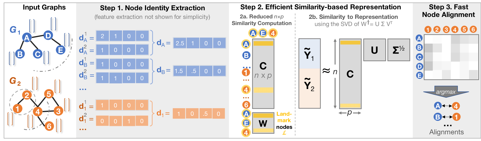
Figure 2. Proposed REGAL approach, consisting of 3 main steps. In the example, for the structural identity, up to $K=2$ hop away neighborhoods are taken into account (the 1-hop and 2-hop neighborhoods for nodes $A$ and $1$ are shown with dashed and dash-dotted lines, respectively). The discount factor is set to $\delta=0.5$. For simplicity, no logarithmic binning is applied on $\mathbf{d}^{k}_{u}$.

3. REGAL: REpresentation Learning-based Graph ALignment

In this section we introduce our representation learning-based network alignment framework, REGAL, for Problem 1. For simplicity we focus on aligning two graphs (e.g., social or protein networks), though our method can easily be extended to more networks. Let $G_{1}(\mathcal{V}_{1},\mathcal{E}_{1})$ and $G_{2}(\mathcal{V}_{2},\mathcal{E}_{2})$ be two unweighted and undirected graphs with node sets $\mathcal{V}_{1}$ and $\mathcal{V}_{2}$; edge sets $\mathcal{E}_{1}$ and $\mathcal{E}_{2}$; and possibly node attributes $\mathcal{A}_{1}$ and $\mathcal{A}_{2}$, respectively. Note that these graphs do not have to be the same size, unlike many other network alignment formulations that have this (often unrealistic) restriction. Let $n$ be the number of nodes across graphs, i.e., $n=|\mathcal{V}_{1}|+|\mathcal{V}_{2}|$. We define the main symbols in Table 3.

The steps of REGAL may be summarized as:

1. Node Identity Extraction: The first step extracts structure- and attribute-related information for all $n$ nodes.

2. Efficient Similarity-based Representation: The second step obtains the node embeddings, conceptually by factorizing a similarity matrix of the node identities from the previous step. To avoid the expensive computation of pairwise node similarities and explicit factorization, we extend the Nyström method for low-rank matrix approximation to perform an implicit similarity matrix factorization by (a) comparing the similarity of each node only to a sample of $p\ll n$ “landmark” nodes, and (b) using these node-to-landmark similarities to construct our representations from a decomposition of its low-rank approximation.

3. Fast Node Representation Alignment: Finally, we align nodes between graphs by greedily matching the embeddings with an efficient data structure that allows for fast identification of the top-$\alpha$ most similar embeddings from the other graph(s).

In the rest of this section we discuss and justify each step of REGAL, the pseudocode of which is given in Algorithm 1. Note that the first two steps, which output a set of node embeddings, comprise our xNetMF method, which may be independently used, particularly for further cross-network analysis tasks.

Table 3. Major symbols and definitions.

Symbols	Definitions
$G_{i}(\mathcal{V}_{i},\mathcal{E}_{i},\mathcal{A}_{i})$	graph $i$ with nodeset $\mathcal{V}_{i}$, edgeset $\mathcal{E}_{i}$, and node attributes $\mathcal{A}_{i}$
$\mathbf{A}_{i}$	adjacency matrix of $G_{i}$
$n_{i}$	number of nodes in graph $G_{i}$
$\mathcal{V}=\mathcal{V}_{1}\cup\mathcal{V}_{2}$	combined set of vertices in $G_{1}$ and $G_{2}$
$|\mathcal{V}|=n$	total number of nodes in graphs $G_{1}$ and $G_{2}$
$d_{\text{avg}}$	average node degree
${\mathcal{R}_{u}^{k}}$	set of $k$-hop neighbors of node $u$
$\mathbf{d}^{k}_{u}$	vector of node degrees in a single set $\mathcal{R}_{u}^{k}$
$K$	maximum hop distance considered
$\delta$	discount factor in $(0,1]$ for distant neighbors
$\mathbf{d}_{u}$	$=\sum_{k=1}^{K}\delta^{k-1}\mathbf{d}^{k}_{u}$ combined neighbor degree vector for node $u$
$b$	number of buckets for degree binning
$\mathbf{f}_{u}$	$F$-dimensional attribute vector for node $u$
$\mathbf{S},\tilde{\mathbf{S}}$	combined structural and attribute-based similarity matrix, and its approximation
$\mathbf{Y},\tilde{\mathbf{Y}}$	matrix with node embeddings as rows, and its approximation
$p$	number of landmark nodes in REGAL
$\alpha$	the number of alignments to find per node

3.1. Step 1: Node Identity Extraction

The goal of REGAL’s representation learning module, xNetMF, is to define node “identity” in a way that generalizes to multi-network problems. This step is critical because many existing works define identity based on node-to-node proximity, but in multi-network problems nodes have no direct connections to each other and thus cannot be sampled in each other’s contexts by random walks on separate graphs. To overcome this problem, we focus instead on more broadly comparable, generalizable quantities: structural identity, which relates to structural roles (Henderson et al., 2012), and attribute-based identity.

Structural Identity. In network alignment, the well-established assumption is that aligned nodes have similar structural connectivity or degrees (Koutra et al., 2013a; Zhang and Tong, 2016). Adhering to this assumption, we propose to learn about a node’s structural identity from the degrees of its neighbors. To gain higher-order information, we also consider neighbors up to $k$ hops from the original node.

For a node $u\in\mathcal{V}$, we denote $\mathcal{R}_{u}^{k}$ as the set of nodes that are exactly $k\geq 0$ steps away from $u$ in its graph $G_{i}$. We want to capture degree information about the nodes in $\mathcal{R}_{u}^{k}$. A basic approach would be to store the degrees in a $D$-dimensional vector $\mathbf{d}^{k}_{u}$, where $D$ is the maximum degree in the original graph $G$, with the $i$-th entry of $\mathbf{d}^{k}_{u}$, or $d_{u}^{k}(i)$, the number of nodes in $\mathcal{R}_{u}^{k}$ with degree $i$. For simplicity, an example of this approach is shown for the vectors $\mathbf{d}_{A},\mathbf{d}_{B}$, etc. in Fig. 2. However, real graphs have skewed degree distributions. To prevent one high-degree node from inflating the length of these vectors, we bin nodes together into $b=\lceil\log_{2}D\rceil$ logarithmically scaled buckets such that the $i$-th entry of $\mathbf{d}^{k}_{u}$ contains the number of nodes $u\in\mathcal{R}_{u}^{k}$ such that $\lfloor\log_{2}(deg(u))\rfloor=i$. This has two benefits: (1) it shortens the vectors $\mathbf{d}^{k}_{u}$ to a manageable $\lceil\log_{2}D\rceil$ dimensions, and (2) it makes their entries more robust to small changes in degree introduced by noise, especially for high degrees when more different degree values are combined into one bucket.

Attribute-Based Identity. Node attributes, or features, have been shown to be useful for cross-network tasks (Zhang and Tong, 2016). Given $F$ node attributes, we can create for each node $u$ an $F$-dimensional vector $\mathbf{f}_{u}$ representing its values (or lack thereof). For example, $f_{u}(i)$ corresponds to the $i^{th}$ attribute value for node $u$. Since we focus on node representations, we mainly consider node attributes, although we note that statistics such as the mean or standard deviation of edge attributes on incident edges to a node can easily be turned into node attributes. Note that while REGAL is flexible to incorporate attributes, if available, it can also rely solely on structural information when such side information is not available.

Cross-Network Node Similarity. We now incorporate the above aspects of node identity into a combined similarity function that can be used to compare nodes within or across graphs, relying on the comparable notions of structural and attribute identity, rather than direct proximity of any kind:

(1) $$\text{sim}(u,v)=\exp{[-\gamma_{s}\cdot||\mathbf{d}_{u}-\mathbf{d}_{v}||_{2}^{2}-\gamma_{a}\cdot\text{dist}(\mathbf{f}_{u},\mathbf{f}_{v})],}$$

where $\gamma_{s}$ and $\gamma_{a}$ are scalar parameters controlling the effect of the structural and attribute-based identity respectively; $\text{dist}(\mathbf{f}_{u},\mathbf{f}_{v})$ is the attribute-based distance of nodes $u$ and $v$, discussed below (this term is ignored if there are no attributes); $\mathbf{d}_{u}=\sum_{k=1}^{K}\delta^{k-1}\mathbf{d}^{k}_{u}$ is the neighbor degree vector for node $u$ aggregated over $K$ different hops; $\delta\in(0,1]$ is a discount factor for greater hop distances; and $K$ is a maximum hop distance to consider (up to the graph diameter). Thus, we compare structural identity at several levels by combining the neighborhood degree distributions at several hop distances, attenuating the influence of distant neighborhoods with a weighting schema that is often encountered in diffusion processes (Koutra et al., 2013b).

The distance between attribute vectors depends on the type of node attributes (e.g., categorical, real-valued). A variety of functions can be employed accordingly. For categorical attributes, which have been studied in attributed network alignment (Zhang and Tong, 2016), we propose using the number of disagreeing features as a attribute-based distance measure of nodes $u$ and $v$: $\text{dist}(\mathbf{f}_{u},\mathbf{f}_{v})=\textstyle\sum_{i=1}^{F}\mathds{1}_{f_{u}(i)\neq f_{v}(i)},$ where $\mathds{1}$ is the indicator function. Real-valued attributes can be compared by Euclidean or cosine distance, for example.

3.2. Step 2: Efficient Similarity-based Representation

As we have mentioned, many representation learning methods are stochastic (Tang et al., 2015; Perozzi et al., 2014; Wang et al., 2016; Grover and Leskovec, 2016; Ribeiro et al., 2017). A subset of these rely on random walks on the original graph (Perozzi et al., 2014; Grover and Leskovec, 2016) or a generated multi-layer similarity graph (Ribeiro et al., 2017)) to sample context for the SGNS embedding model. For cross-network analysis, we avoid random walks for two reasons: (1) The variance they introduce in the representation learning often makes embeddings across different networks non-comparable (Heimann and Koutra, 2017); and (2) they can add to the computational expense. For example, node2vec’s total runtime is dominated by its sampling time (Grover and Leskovec, 2016).

To overcome the aforementioned issues, we propose a new implicit matrix factorization-based approach that leverages a combined structural and attribute-based similarity matrix $\mathbf{S}$, which is induced by our similarity function in Eq. (1) and considers affinities at different neighborhoods. Intuitively, the goal is to find $n\times p$ matrices $\mathbf{Y}$ and $\mathbf{Z}$ such that: $\mathbf{S}\approx\mathbf{Y}\mathbf{Z}^{\top}$, where $\mathbf{Y}$ is the node embedding matrix and $\mathbf{Z}$ is not needed for our purposes. We first discuss the limitations of traditional approaches, then propose an efficient way of obtaining the embeddings without ever explicitly computing $\mathbf{S}$.

Limitations of Existing Approaches. A natural but naïve approach is to compute combined structural and attribute-based similarities between all pairs of nodes within and across both graphs to form the matrix $\mathbf{S}$, such that $\mathbf{S}_{ij}=sim(i,j)\;\forall i,j\in\mathcal{V}$. Then $\mathbf{S}$ can be explicitly factorized, for example by minimizing a factorization loss function given $\mathbf{S}$ as input, (e.g., the Frobenius norm $||\mathbf{S}-\mathbf{Y}\mathbf{Z}^{\top}||_{F}^{2}$ (Lee and Seung, 2001)). However, both the computation and storage of $\mathbf{S}$ have quadratic complexity in $n$. While this would allow us to embed graphs jointly, it lacks the needed scalability for multiple large networks.

Another alternative is to create a sparse similarity matrix by calculating only the “most important” similarities, for each node choosing a small number of comparisons using heuristics like similarity of node degree (Ribeiro et al., 2017). However, such ad-hoc heuristics may be fragile in the context of noise. We will have no approximation at all for most of the similarities, and there is no guarantee that the most important ones are computed.

Step 2a: Reduced $n\times p$ Similarity Computation. Instead, we propose a principled way of approximating the full similarity matrix $\mathbf{S}$ with a low-rank matrix $\tilde{\mathbf{S}}$, which is never explicitly computed. To do so, we randomly select $p\ll n$ “landmark” nodes chosen across both graphs $G_{1}$ and $G_{2}$ and compute their similarities to all $n$ nodes in these graphs using Eq. (1). This yields an $n\times p$ similarity matrix $\mathbf{C}$, from which we can extract a $p\times p$ “landmark-to-landmark” submatrix $\mathbf{W}$. As we explain below, these two matrices suffice to approximate the full similarity matrix and allow us to obtain node embeddings without actually computing and factorizing $\tilde{\mathbf{S}}$.

To do so, we extend the Nyström method, which has applications in randomized matrix methods for kernel machines (Drineas and Mahoney, 2005), to node embedding. The low-rank matrix $\tilde{\mathbf{S}}$ is given as:

(2) $$\tilde{\mathbf{S}}=\mathbf{C}\mathbf{W}^{\dagger}\mathbf{C}^{\top},$$

where $\mathbf{C}$ is an $n\times p$ matrix formed by sampling $p$ landmark nodes from $\mathcal{V}$ and computing the similarity of all $n$ nodes of $G_{1}$ and $G_{2}$ to the $p$ landmarks only, as shown in Fig. 2. Meanwhile, $\mathbf{W}^{\dagger}$ is the pseudoinverse of $\mathbf{W}$, a $p\times p$ matrix consisting of the pairwise similarities among the landmark nodes (it corresponds to a subset of $p$ rows of $\mathbf{C}$). We choose landmarks randomly; more elaborate (and slower) sampling techniques based on leverage scores (Alaoui and Mahoney, 2015) or node centrality measures offer little, if any, performance improvement.

Because $\tilde{\mathbf{S}}$ contains an estimate for the similarity between any pair of nodes in either graph, it would still take $\Omega(n^{2})$ time and space to compute and store. However, as we discuss below, to learn node representations we never have to explicitly construct $\tilde{\mathbf{S}}$ either.

Step 2b: From Similarity to Representation. Recall that our ultimate interest is not in the similarity matrix $\mathbf{S}$ or even an approximation such as $\tilde{\mathbf{S}}$, but in the node embeddings that we can obtain from a factorization of the latter. We now show that we can actually obtain these from the decomposition in Eq. (2):

Theorem 3.1.

Given graphs $G_{1}(\mathcal{V}_{1},\mathcal{E}_{1})$ and $G_{2}(\mathcal{V}_{2},\mathcal{E}_{2})$ with $n\times n$ joint combined structural and attribute-based similarity matrix $\mathbf{S}\approx\mathbf{Y}\mathbf{Z}^{T}$, its node embedding matrix $\mathbf{Y}$ can be approximated as

$$\tilde{\mathbf{Y}}=\mathbf{C}\mathbf{U}\mathbf{\Sigma}^{1/2},$$

where $\mathbf{C}$ is the $n\times p$ matrix of similarities between the $n$ nodes and $p$ randomly chosen landmark nodes, and $\mathbf{W}^{\dagger}=\mathbf{U}\mathbf{\Sigma}\mathbf{V}^{\top}$ is the full rank singular value decomposition of the pseudoinverse of the small $p\times p$ landmark-to-landmark similarity matrix $\mathbf{W}$.

Proof.

Given the full-rank SVD of the $p\times p$ matrix $\mathbf{W}^{\dagger}$ as $\mathbf{U}\mathbf{\Sigma}\mathbf{V}^{\top},$ we can rewrite Eq. (2) as $\mathbf{S}\approx\tilde{\mathbf{S}}=\mathbf{C}(\mathbf{U}\mathbf{\Sigma}\mathbf{V}^{\top})\mathbf{C}^{\top}=(\mathbf{C}\mathbf{U}\mathbf{\Sigma}^{1/2})\cdot(\mathbf{\Sigma}^{1/2}\mathbf{V}^{\top}\mathbf{C}^{\top})=\tilde{\mathbf{Y}}\tilde{\mathbf{Z}}^{\top}$. ∎

Now, we never have to construct an $n\times n$ matrix and then factorize it (i.e., by optimizing a nonconvex factorization objective). Instead, to derive $\tilde{\mathbf{Y}}$, the only node comparisons we need are for the $n\times p$ “skinny” matrix $\mathbf{C}$, while the expensive SVD is performed only on its small submatrix $\mathbf{W}$. Thus, we can obtain node representations by implicitly factorizing $\tilde{\mathbf{S}}$, a low-rank approximation of the full similarity matrix $\mathbf{S}$. The $p$-dimensional node embeddings of the two input graphs $G_{1}$ and $G_{2}$ are then subsets of $\tilde{\mathbf{Y}}$: $\tilde{\mathbf{Y}}_{1}$ and $\tilde{\mathbf{Y}}_{2}$, respectively. This construction corresponds to the explicit factorization (Fig. 3), but at significant runtime and storage savings.

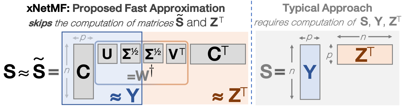
Figure 3. Proposed xNetMF (using the SVD of $\mathbf{W}^{\dagger}$) vs. typical matrix factorization for computing the node embeddings $\mathbf{Y}$. Our xNetMF method leads to significant savings in space and runtime.

As stated earlier, xNetMF, which we summarize in Alg. 2, forms the first two steps of REGAL. The postprocessing step, where we normalize the magnitude of the embeddings, makes them more comparable based on Euclidean distance, which we use in REGAL.

Connection between xNetMF and SGNS. We show a formal connection between matrix factorization, the technique behind our xNetMF, and a variant of the struc2vec framework: another form of structure-based embedding optimized with SGNS (Ribeiro et al., 2017) in Appendix A. Indeed, similar equivalences between SGNS and matrix factorization have been studied (Levy and Goldberg, 2014; Li et al., 2015) and applied to proximity-based node embedding methods (Qiu et al., 2018), but ours is the first to explore such connections for methods that preserve structural identity.

Algorithm 1 REGAL ($G_{1},G_{2}$, $p,K,\gamma_{s},\gamma_{a},\alpha$)

1:====== STEPS 1 and 2. Structural Node Representation Learning ======

2:$[\tilde{\mathbf{Y}}_{1},\tilde{\mathbf{Y}}_{2}]$ = xNetMF ($G_{1},G_{2},p,K,\gamma_{s},\gamma_{a}$) $\triangleright$ Learn $n_{1}\times p$ and $n_{2}\times p$ embeddings

3:=========== STEP 3. Fast Node Representation Alignment ===========

4:$\mathbf{M}$ = empty $\triangleright$ sparse $n_{1}\times n_{2}$ matrix $\mathbf{M}$ of possible alignments

5:$T$ = KDTree($\tilde{\mathbf{Y}}_{2}$) $\triangleright$ Build a $k$-d tree on the node embeddings of $G_{2}$

6:/* Match embeddings to infer alignments */

7:for $i=1\to n_{1}$ do

8:    /* For embedding $i$ in $G_{1}$, get the $\alpha$ most similar embed. in $G_{2}$ and distances*/

9:    [TOP-$\alpha$, TOP-dist] = QueryKDTree(T, $\tilde{\mathbf{Y}}_{1}[i]$, $\alpha$) $\triangleright$ $\tilde{\mathbf{Y}}_{1}[i]$: $i^{th}$ embedding

10:    for $j$ in TOP-$\alpha$ do

11:        $m_{ij}=e^{-\text{TOP-dist}[j]}$ $\triangleright$ Populating alignment matrix $\mathbf{M}$ with embed.

12:    end for$\triangleright$ similarities: $e^{\text{TOP-dist}[j]}=e^{-||\,\tilde{\mathbf{Y}}_{1}[i]\,-\,\tilde{\mathbf{Y}}_{2}[j]\,||_{2}^{2}}$

13:end for

14:return $\mathbf{M}$ $\triangleright$ alignments are largest entries in each row or column (Fig. 1)

Algorithm 2 xNetMF ($G_{1},G_{2},p,K,\gamma_{s},\gamma_{a}$)

1:================ STEP 1. Node Identity Extraction ================

2:for node $u$ in $\mathcal{V}_{1}\cup\mathcal{V}_{2}$ do

3:    for hop $k$ up to $K$ do $\triangleright$ counts of node degrees of $k$-hop neighbors of $u$

4:        $\mathbf{d}^{k}_{u}$ = CountDegreeDistributions($\mathcal{R}_{u}^{k}$) $\triangleright$ $1\leq K\leq\text{graph diameter}$

5:    end for

6:    $\mathbf{d}_{u}=\sum_{k=1}^{K}\delta^{k-1}\mathbf{d}^{k}_{u}$ $\triangleright$ discount factor $\delta\in(0,1]$

7:end for

8:========= STEP 2. Efficient Similarity-based Representation =========

9:========== STEP 2a. Reduced $n\times p$ Similarity Computation ==========

10:$\mathcal{L}=$ ChooseLandmarks($G_{1},G_{2}$,$p$) $\triangleright$ choose $p$ nodes from $G_{1}$, $G_{2}$

11:for node $u$ in $\mathcal{V}$ do

12:    for node $v$ in $\mathcal{L}$ do

13:        $c_{uv}=e^{-\gamma_{s}\cdot||\mathbf{d}_{u}-\mathbf{d}_{v}||_{2}^{2}\,-\,\gamma_{a}\cdot\text{dist}(\mathbf{f}_{u},\mathbf{f}_{v})}$

14:    end for

15:end for$\triangleright$ Used in low-rank approx. of similarity graph (not constructed)

16:=========== STEP 2b. From Similarity to Representation ============

17:$\mathbf{W}=\mathbf{C}[\mathcal{L},\mathcal{L}]$ $\triangleright$ Rows of $\mathbf{C}$ corresponding to landmark nodes

18:$[\mathbf{U},\mathbf{\Sigma},\mathbf{V}]$ = SVD($\mathbf{W}^{\dagger}$)

19:$\tilde{\mathbf{Y}}=\mathbf{C}\mathbf{U}\mathbf{\Sigma}^{-\frac{1}{2}}$ $\triangleright$ Embedding: implicit factorization of similarity graph

20:$\tilde{\mathbf{Y}}=Normalize(\tilde{\mathbf{Y}})$ $\triangleright$ Postprocessing: make embeddings have magnitude 1

21:$\tilde{\mathbf{Y}}_{1},\tilde{\mathbf{Y}}_{2}$ = Split($\tilde{\mathbf{Y}}$) $\triangleright$ Separate representations for nodes in $G_{1}$, $G_{2}$

22:return $\tilde{\mathbf{Y}}_{1},\tilde{\mathbf{Y}}_{2}$

3.3. Step 3: Fast Node Representation Alignment

The final step of REGAL is to efficiently align nodes using their representations, assuming that two nodes $u\in\mathcal{V}_{1}$ and $v\in\mathcal{V}_{2}$ may match if their xNetMF embeddings are similar. Let $\tilde{\mathbf{Y}}_{1}$ and $\tilde{\mathbf{Y}}_{2}$ be matrices of the $p$-dimensional embeddings for nodes in graphs $G_{1}$ and $G_{2}$. We take the likeliness of (soft) alignment to be proportional to the similarity between the nodes’ embeddings. Thus, we greedily align nodes to their closest match in the other graph based on embedding similarity, as shown in Fig. 2. This method is simpler and faster than optimization-based approaches, and works thanks to high-quality node feature representations.

Data structures for efficient alignment. A natural way to find the alignments for each node is to compute all pairs of similarities between node embeddings (i.e., the rows of $\tilde{\mathbf{Y}}_{1}$ and $\tilde{\mathbf{Y}}_{2}$) and choose the top-1 for each node. Of course, this is not desirable due to its inefficiency. Since in practice only the top-$\alpha$ most likely alignments are used, we turn to specialized data structures for quickly finding the closest data points. We store the embeddings $\tilde{\mathbf{Y}}_{2}$ in a $k$-d tree, a data structure used to accelerate exact similarity search for nearest neighbor algorithms and many other applications (Bhatia et al., 2010).

For each node in $G_{1}$, we can quickly query this tree with its embedding to find the $\alpha<<n$ closest embeddings from nodes in $G_{2}$. This allows us to compute “soft” alignments for each node by returning one or more nodes in the opposite graph with the most similar embeddings, unlike many existing alignment methods that only find “hard” alignments (Bayati et al., 2013; Zhang and Tong, 2016; Singh et al., 2008; Klau, 2009). Here, we define the similarity between the $p$-dimensional embeddings of nodes $u$ and $v$ as $sim_{emb}(\tilde{\mathbf{Y}}_{1}[u],\tilde{\mathbf{Y}}_{2}[v])=e^{-||\,\tilde{\mathbf{Y}}_{1}[u]\,-\,\tilde{\mathbf{Y}}_{2}[v]\,||_{2}^{2}}$, which converts the Euclidean distance to similarity. Since we only want to align nodes to counterparts in the other graph, we only compare embeddings in $\tilde{\mathbf{Y}}_{1}$ with ones in $\tilde{\mathbf{Y}}_{2}$. If multiple top alignments are desired, they may be returned in sorted order by their embedding similarity; we use sparse matrix notation in the pseudocode just for simplicity.

3.4. Complexity Analysis

Here we analyze the computational complexity of each step of REGAL. To simplify notation, we assume both graphs have $n_{1}=n_{2}=n^{\prime}$ nodes.

1. Extracting node identity: It takes approximately $O(n^{\prime}Kd_{avg}^{2})$ time, finding neighborhoods up to hop distance $K$ by joining the neighborhoods of neighbors at the previous hop: formally, we can construct $\mathcal{R}_{u}^{k}=\bigcup_{v\in\mathcal{R}_{u}^{k-1}}\mathcal{R}_{v}^{1}-\bigcup_{i=1}^{k-1}\mathcal{R}_{u}^{i}$. We could also use breadth-first search from each node to compute the $k$-hop neighborhoods in $O(n^{\prime 3})$ worst case time—in practice significantly lower for sparse graphs and/or small $K$—but we find that this construction is faster in practice.

2. Computing similarities: We compute the similarities of the length-$b$ features (weighted counts of node degrees in the k-hop neighborhoods, split into $b$ buckets) between each node and $p$ landmark nodes: this takes $O(n^{\prime}pb)$ time.

3. Obtaining representations: We first compute the pseudoinverse and SVD of the $p\times p$ matrix $\mathbf{W}$ in time $O(p^{3})$, and then left multiply it by $\mathbf{C}$ in time $O(n^{\prime}p^{2})$. Since $p<<n^{\prime}$, the total time complexity for this step is $O(n^{\prime}p^{2})$.

4. Aligning embeddings: We construct a $k$-d tree and use it to find the top alignment(s) in $G_{2}$ for each of the $n^{\prime}$ nodes in $G_{1}$ in average-case time complexity $O(n^{\prime}\log n^{\prime})$.

The total complexity is $O(n^{\prime}\max\{pb,p^{2},Kd_{avg}^{2},\log n^{\prime}\})$. As we show experimentally, it suffices to choose small $K$ as well as $p$ and $b$ logarithmic in $n^{\prime}$. With $d_{avg}$ often being small in practice, this can yield sub-quadratic time complexity. It is straightforward to show that the space requirements are sub-quadratic as well.

4. Experiments

We answer three important questions about our methods:
(Q1) How does REGAL compare to baseline methods for network alignment on noisy real world datasets (Table 5), with and without attribute information, in terms of accuracy and runtime?
(Q2) How scalable is REGAL?
(Q3) How sensitive are REGAL and xNetMF to hyperparameters?

Experimental Setup. Following the network alignment literature (Koutra et al., 2013a; Zhang and Tong, 2016), for each real network dataset with adjacency matrix $\mathbf{A}$, we generate a new network with adjacency matrix $\mathbf{A}^{\prime}=\mathbf{P}\mathbf{A}\mathbf{P}^{\top}$, where $\mathbf{P}$ is a randomly generated permutation matrix with the nonzero entries representing ground-truth alignments. We add structural noise to $\mathbf{A}^{\prime}$ by removing edges with probability $p_{s}$ without disconnecting any nodes.

For experiments with attributes, we generate synthetic attributes for each node if the graph does not have any. We add noise to these by flipping binary values or choosing categorical attribute values uniformly at random from the remaining possible values with probability $p_{a}$. For each dataset and noise level, noise is randomly and independently added.

All experiments are performed on an Intel(R) Xeon(R) CPU E5-1650 at 3.50GHz with 256GB RAM, with hyperparameters $\delta=0.01$, $K=2$, $\gamma_{s}=\gamma_{a}=1$, and $p=\lfloor 10\log_{2}n\rfloor$ unless otherwise stated. Landmarks for REGAL are chosen arbitrarily from among the nodes in our graphs, in keeping with the effectiveness and popularity of sampling uniformly at random (Drineas and Mahoney, 2005). In Sec. 4.3, we explore the parameter choices and find that these settings yield stable results at reasonable computational cost.

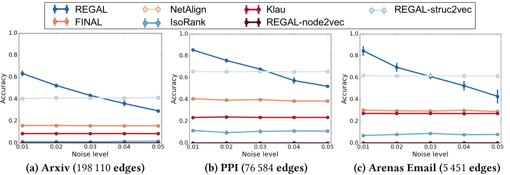
Figure 4. Accuracy of network alignment methods with varying $p_{s}$. REGAL (in dark blue) achieves consistently high accuracy and runs faster than its closest competitors (Table 4).

Table 4. Average (stdev) runtime in sec of alignment methods from 5 trials. The two fastest methods per dataset are in bold. REGAL is faster than its closest competitors in accuracy (Fig. 4).

Dataset	Arxiv	PPI	Arenas
FINAL	4182 (180)	62.88 (32.20)	3.82 (1.41)
NetAlign	149.62 (282.03)	22.44 (0.61)	1.89 (0.07)
IsoRank	17.04 (6.22)	6.14 (1.33)	0.73 (0.05)
Klau	1291.00 (373)	476.54 (8.98)	43.04 (0.80)
REGAL-node2vec	709.04 (20.98)	139.56 (1.54)	15.05 (0.23)
REGAL-struc2vec	1975.37 (223.22)	441.35 (13.21)	74.07 (0.95)
REGAL	86.80 (11.23)	18.27 (2.12)	2.32 (0.31)

Baselines. We compare against six baselines. Four are well known existing network alignment methods and two are variants of our proposed framework that match embeddings produced by existing node embedding methods (i.e., not xNetMF). The four existing network alignment methods are: (1) FINAL, which introduces a family of algorithms optimizing quadratic objective functions (Zhang and Tong, 2016); (2) NetAlign, which formulates alignment as an integer quadratic programming problem and solves it with message passing algorithms (Bayati et al., 2013); (3) IsoRank, which solves a version of the integer quadratic program with relaxed constraints (Singh et al., 2008); and (4) Klau’s algorithm (Klau), which imposes a linear programming relaxation, decomposes the symmetric constraints and solves it iteratively (Klau, 2009). These methods all require as input a matrix containing prior alignment information, which we construct from degree similarity, taking the top $\lfloor\log_{2}n\rfloor$ entries for each node; REGAL, by contrast, does not require prior alignment information.

For the two variants of our framework, which we refer to as (5) REGAL-node2vec and (6) REGAL-struc2vec, we replace our own xNetMF embedding step (i.e., Steps 1 and 2 in REGAL) with existing node representation learning methods node2vec (Grover and Leskovec, 2016) or struc2vec (Ribeiro et al., 2017): two recent, state-of-the-art node embedding methods that make a claim about being able to capture some form of structural equivalence. To apply these embedding methods, which were formulated for a single network, we create a single input graph $G$ by combining the graphs with respective adjacency matrices $\mathbf{A}$ and $\mathbf{A}^{\prime}$ into one block-diagonal adjacency matrix $[\mathbf{A}\;\mathbf{0};\mathbf{0}\;\mathbf{A}^{\prime}]$. Beyond the input, we use their default parameters: 10 random walks of length 80 for each node to sample context with a window size of 10. For node2vec, we set $p=q=1$ (other values make little difference). For struc2vec, we use the recommended optimizations (Ribeiro et al., 2017) to compress the degree sequences and reduce the number of node comparisons, which were found to speed up computation with little effect on performance (Ribeiro et al., 2017). As we do for our xNetMF method, we consider a maximum hop distance of $K=2$.

Metrics. We compare REGAL to baselines with two metrics: alignment accuracy, which we take as (# correct alignments) / (total # alignments), and runtime. When computing results, we average over 5 independent trials on each dataset at each setting (with different random permutations and noise additions) and report the mean result and the standard deviation (as bars around each point in our plots.) We also show where REGAL’s soft alignments contain the “correct” similarities within its top $\alpha<<n$ choices using the more general top-$\alpha$ accuracy: (# correct alignments in top-$\alpha$ choices) / (total # alignments). This metric does not apply to the existing network alignment baselines that do not directly match node embeddings and only find hard alignments.

Table 5. Real data used in our experiments.

Name	Nodes	Edges	Description
Facebook (Viswanath et al., 2009)	63 731	817 090	social network
Arxiv (Leskovec and Krevl, 2014)	18 722	198 110	collaboration network
DBLP (Prado et al., 2013)	9 143	16 338	collaboration network
PPI (Breitkreutz et al., 2008)	3 890	76 584	protein-protein interaction
Arenas Email (Kunegis, 2013)	1 133	5 451	communication network

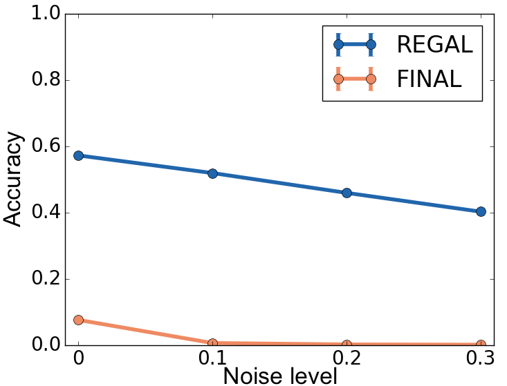
(a) 1 synthetic binary attribute

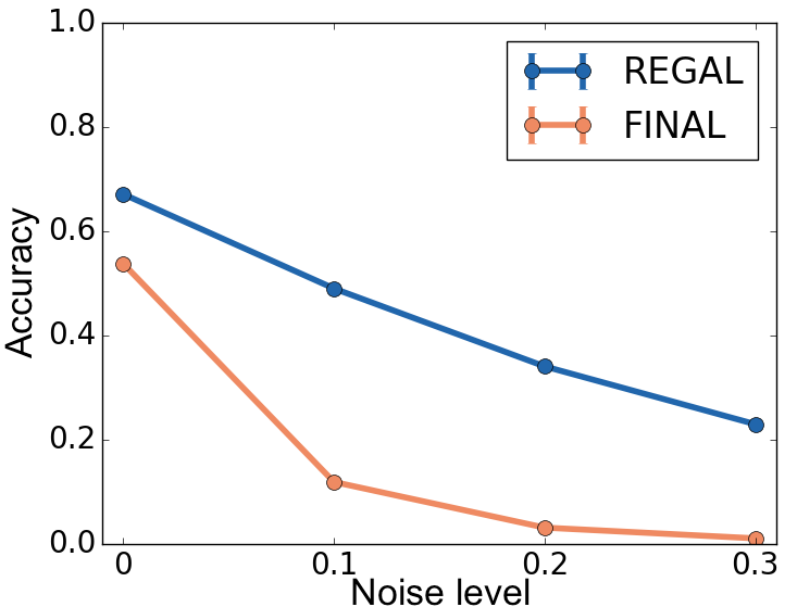
(b) 3 synthetic binary attributes

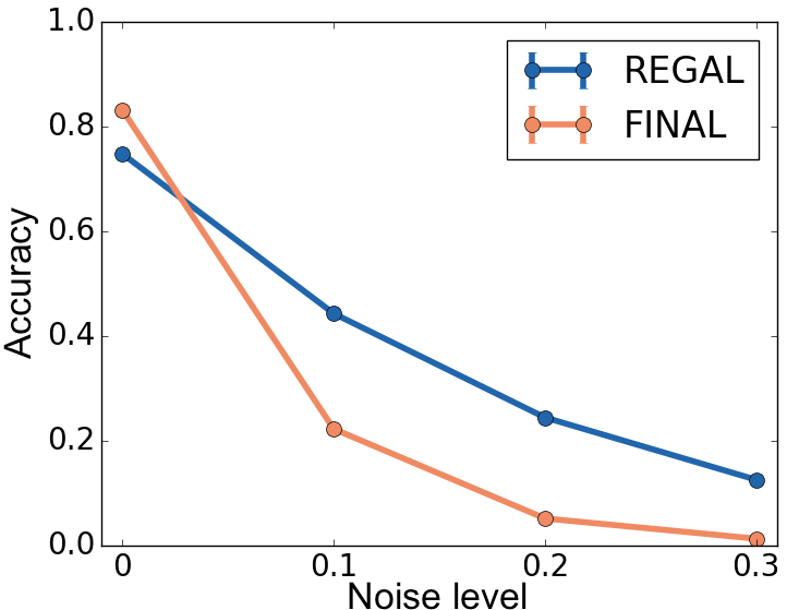
(c) 5 synthetic binary attributes

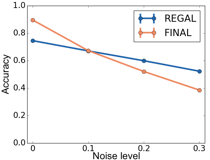
(d) Real attribute (29 values)

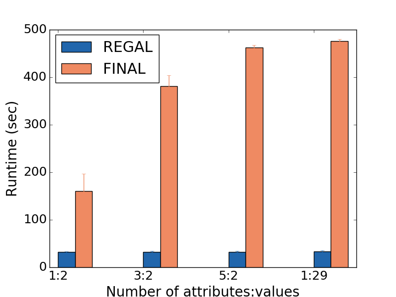
(e) Runtime with attributes

Figure 5. DBLP Network alignment with varying $p_{a}$: REGAL is more robust to attribute noise (plots a-d) and runs faster (plot e) than FINAL for various numbers and types of attributes. In (e) the x axis consists of $<$# of attributes: # of values$>$ pairs corresponding to plots (a)-(d).

4.1. Q1: Comparative Alignment Performance

To assess the comparative performance of REGAL versus existing network alignment methods on a variety of challenging datasets, we perform two experiments studying the effects of structural and attribute noise, respectively.

4.1.1. Effects of structural noise.

In this experiment we study how well REGAL matches nodes based on structural identity alone. This also allows us to compare to the baseline network alignment methods NetAlign, IsoRank, and Klau, as well as the node embedding methods node2vec and struc2vec, none of which was formulated to handle or align attributed graphs (which we study in Sec. 4.1.2). As we discuss further below, REGAL is one of the fastest network alignment methods, especially on large datasets, and has comparable or better accuracy than all baselines.

Results. (1) Accuracy. The accuracy results on several datasets are shown in Figure 4. The structural embedding REGAL variants consistently perform best. Both REGAL (matching our proposed xNetMF embeddings) and REGAL-struc2vec are significantly more accurate than all non-representation learning baselines across noise levels and datasets. As expected, REGAL-node2vec does hardly better than random chance because rather than preserving structural similarity, it preserves similarity to nodes based on their proximity to each other, which means there is no way of identifying similarity to corresponding nodes in other, disconnected graphs (even when we combine them into one large graph, because they form disconnected components.) This major limitation of embedding methods that use proximity-based node similarity criteria (Heimann and Koutra, 2017) justifies the need for structural embeddings for cross-network analysis.

Between REGAL and REGAL-struc2vec, the two highest performers, REGAL performs better with lower amounts of noise. This is likely because struc2vec’s randomized context sampling introduces some variance into the representations that xNetMF does not have, as nodes that should match will have different embeddings not only because of noise, but also because they had different contexts sampled. With higher amounts of noise (4-5%), REGAL outperforms REGAL-struc2vec in speed, but at the cost of some accuracy. It is also worth noting that their accuracy margin is smaller for larger graphs. On larger datasets, our simple and fast logarithmic binning scheme (Step 1 in Sec. 3.1) provides a robust enough way of comparing nodes with high expected degrees. However, on small graphs with a few thousand nodes and edges, it appears that struc2vec’s use of dynamic time warping (DTW) better handles misalignment of degree sequences from noise because it is a nonlinear alignment scheme. Still, we will see that REGAL is significantly faster than its struc2vec variant, since DTW is computationally expensive (Ribeiro et al., 2017), as is context sampling and SGNS training.

(2) Runtime. In Table 4, we compare the average runtimes of all different methods across noise levels. We observe that REGAL scales significantly better using xNetMF than when using other node embedding methods. Notably, REGAL is 6-8$\times$ faster than REGAL-node2vec and 22-31$\times$ faster than REGAL-struc2vec. This is expected as both dynamic time warping (in struc2vec) and context sampling for SGNS (in struc2vec and node2vec) come with large computational costs. REGAL, at the cost of some robustness to high levels of noise, avoids both the variance and computational expense of random-walk-based sampling. This is a significant benefit that allows REGAL to achieve up to an order of magnitude speedup over the other node embedding methods. Additionally, REGAL is able to leverage the power of node representations and also use attributes, unlike the other representation learning methods.

Comparing to baselines that do not use representation learning, we see that REGAL is competitive in terms of runtime as well as significantly more accurate. REGAL is consistently faster than FINAL and Klau, the next two best-performing methods by accuracy (NetAlign is virtually tied for third place with Klau on all datasets). Although NetAlign runs faster than REGAL on small datasets like Arenas, on larger datasets like Arxiv NetAlign’s message passing becomes expensive. Finally, while IsoRank is consistently the fastest method, it performs among the worst on all datasets in accuracy. Thus, we can see that our REGAL framework is also one of the fastest network alignment methods as well as the most accurate.

4.1.2. Effects of attribute-based noise.

In the second experiment, we study REGAL’s comparative sensitivity to $p_{a}$ when we use node attributes. Here we compare REGAL to FINAL because it is the only baseline that handles attributes. We also omit embedding methods othen than xNetMF, since they operate on plain graphs.

We study a subnetwork of a larger DBLP collaboration network extracted in (Zhang and Tong, 2016) (Table 5). This dataset has 1 node attribute with 29 values, corresponding to the top conference in which each author (a node in the network) published. This single attribute is quite discriminatory: with so many possible attribute values, a comparatively smaller number of nodes share the same value. We add $p_{s}=0.01$ structural noise to randomly generated permutations.

We also increase attribute information by increasing the number of attributes. To do so, we simulate different numbers of binary attributes. We study somewhat higher levels of attribute noise, as they are not strictly required for network alignment.

Results. In Figure 5, we see that REGAL mostly outperforms FINAL in the presence of attribute noise (both for real and multiple synthetic attributes), or in the case of limited attribute information (e.g., only 1-3 binary attributes in Fig. 5a-5c). This is because FINAL relies heavily on attributes, whereas REGAL uses structural and attribute information in a more balanced fashion.

While FINAL achieves slightly higher accuracy than REGAL with abundant attribute information from many attributes or attribute values and minimal noise (e.g. the real attribute with 29 values in Figure 5d, or 5 binary attributes in Figure 5c), this is expected due to FINAL’s reliance on attributes. Also, in Figure 5e where we plot the runtime with respect to number of $<$attributes : attribute values$>$, we see FINAL incurs significant runtime increases as it uses extra attribute information. Even without these added attributes, REGAL is up to two orders of magnitude faster than FINAL.

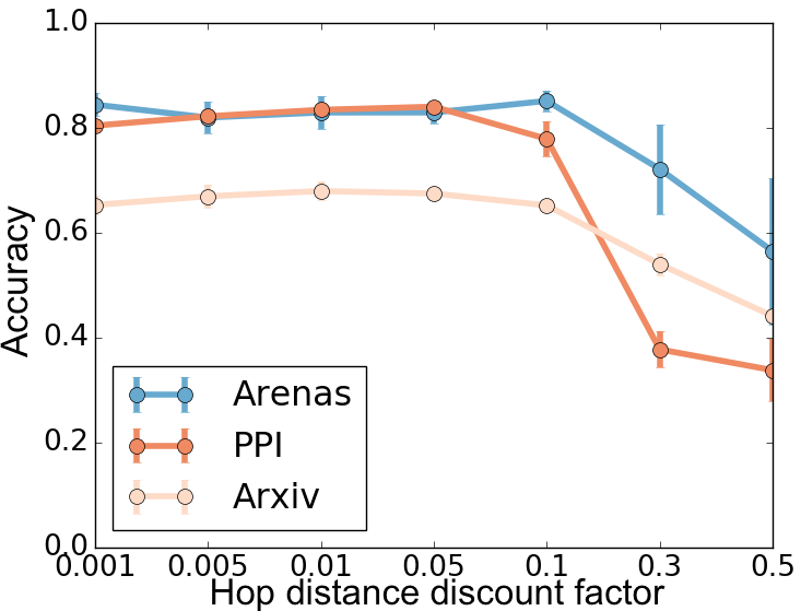
(a) Discount factor $\delta$

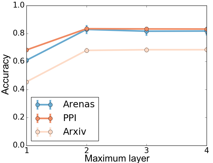
(b) Maximum hop distance $K$

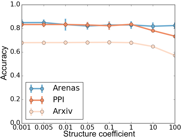
(c) Coeff. $\gamma_{s}$ (structural sim.)

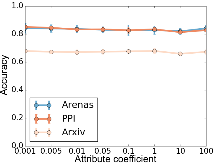
(d) Coeff. $\gamma_{a}$ (attribute sim.)

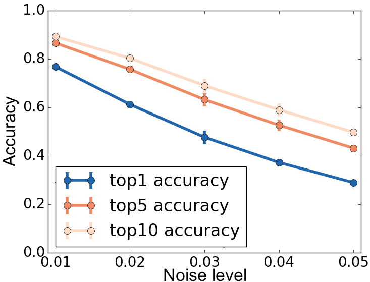
(e) top-$\alpha$ scores on Facebook (Viswanath et al., 2009)

Figure 6. Robustness of REGAL to hyperparameters on different datasets: REGAL is generally robust for a range of values, without fine tuning.

4.2. Q2: Scalability

To analyze the scalability of REGAL, we generate Erdös-Rényi graphs with $n=100$ to 1,000,000 nodes and constant average degree 10, along with one binary attribute. We generate a randomized, noisy permutation ($p_{s}=0.01,p_{a}=0.05$) and look for the top $\alpha=1$ alignments. Thus, we embed both graphs–double the number of nodes in a single graph. Figure 7 shows the runtimes for the major steps of our methods.

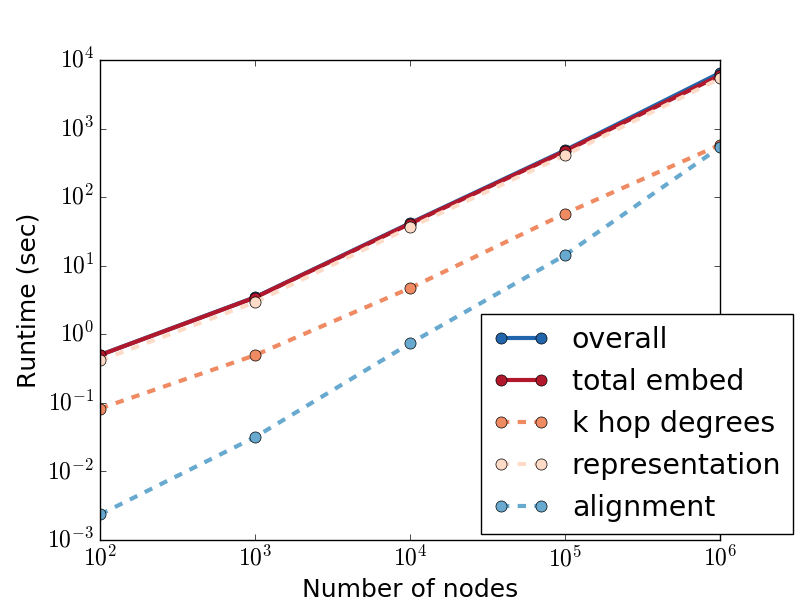
Figure 7. REGAL is subquadratic.

Results. We see that the total runtimes of REGAL’s steps are clearly sub-quadratic, which is rare for alignment tasks. In practice this means that REGAL can scale to very large networks. The dominant step is computing $O(n\log n)$ similarities to landmarks in $\mathbf{C}$ and using this to form the Nyström-based representation. The alignment time complexity grows the most steeply, as the dimensionality $p$ grows with the network size and increasingly affects lookup times. In practice, though, the alignment adds little overhead time, even for the largest graph, because of the $k$-d tree. Without it, REGAL runs out of memory on 100K or more nodes.

From a practical perspective, while our current implementation is single-threaded, many steps—including the expensive embedding construction and alignment steps—are easily and trivially parallelizable, offering possibilities for even greater speedups.

4.3. Q3: Sensitivity Analysis

To understand how REGAL’s hyperparameters affect performance, we analyze accuracy by varying hyperparameters in several experiments. For brevity, we report results at $p_{s}=0.01$ and with a single binary noiseless attribute, although further experiments with different settings yielded similar results. Overall we find that REGAL is robust to different settings and datasets, indicating that REGAL can be applied readily to different graphs without requiring excessive domain knowledge or fine-tuning.

Results. (1) Discount factor $\delta$ and max hop distance $K$. Figures 6a and 6b respectively show the performance of REGAL as a function of $\delta$, the discount factor on further hop distances, and $K$, the maximum hop distance to consider. We find that some higher-order structural information does help (thus $K=2$ performs slightly better than $K=1$), but only up to a point. Beyond approximately 2 layers out, the structural similarity is so tenuous that it primarily adds noise to the neighborhood degree distribution (furthermore, computing further hop distances adds computational expense). Choosing $\delta$ between $0.01$–$0.1$ tends to yield best performance. Larger discount factors $\delta$ tend to do poorly, though extremely small values may lose higher-order structural information.

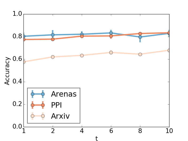
(a) Accuracy w.r.t. # of landmarks

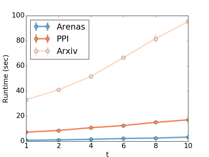
(b) Runtime w.r.t. # of landmarks

Figure 8. Robustness of REGAL to $t$, which controls the number of landmarks $p=\lfloor t\log_{2}n\rfloor$: choosing more landmarks is more computationally expensive but can slightly increase accuracy.

(2) Weights of structural $\gamma_{s}$ and attributed $\gamma_{a}$ similarity. Next, we explore how to set the coefficients on the terms in the similarity function weighting structural and attribute similarity, which also governs a tradeoff between structural and attribute identity. In Figs. 6c and 6d we respectively vary $\gamma_{s}$ and $\gamma_{a}$ while setting the other to be 1. In general, setting these parameters to be 1, our recommended default value, does fairly well. Significantly larger values yield less stable performance.

(3) Dimensionality of embeddings $p$. To study the effects of the rank of the implicit low-rank approximation, which is also the dimensionality of the embeddings, we set the number of landmarks $p$ equal to $\lfloor t\log_{2}n\rfloor$ and vary $t$. Figure 8a shows that the accuracy is generally highest for the highest values of $t$, but Figure 8b shows the expected increase in REGAL’s runtime as more similarities are computed in $\mathbf{C}$ and higher-dimensional embeddings are compared. To spare no expense in maximizing accuracy we use $t=10$. However, fewer landmarks still yield almost as high accuracy if computational constraints or high dimensionality are issues.

(4) Top-$\alpha$ accuracy. It is worth studying not just the proportion of correct hard alignments, but also the top-$\alpha$ scores of the soft alignments that REGAL can return. We perform alignment without attributes on a large Facebook subnetwork (Viswanath et al., 2009) and visualize the top-1, top-5, and top-10 scores in Fig. 6e. Across noise settings, the top-$\alpha$ scores are considerably several percentage points higher than the top-1 scores, indicating that even when REGAL misaligns a node, it often still recognizes the similarity of its true counterpart. REGAL’s ability to find soft alignments could be valuable in many applications, like entity resolution across social networks (Koutra et al., 2013a).

5. Conclusion

Motivated by the numerous applications of network alignment in social, natural, and other sciences, we proposed REGAL, a network alignment framework that leverages the power of node representation learning by aligning nodes via their learned embeddings. To efficiently learn node embeddings that are comparable across multiple networks, we introduced xNetMF within REGAL. To the best of our knowledge, we are the first to propose an unsupervised representation learning-based network alignment method.

Our embedding formulation captures node similarities using structural and attribute identity, making it suitable for cross-network analysis. Unlike other embedding methods that sample node context with computationally expensive and variance-inducing random walks, our extension of the Nyström low-rank approximation allows us to implicitly factorize a similarity matrix without having to fully construct it. Furthermore, we showed that our formulation is a matrix factorization perspective on the skip-gram objective optimized over node context sampled from a similarity graph. Experimental results showed that REGAL is up to 30% more accurate than baselines and $30\times$ faster in the representation learning stage. Future directions include extending our techniques to weighted networks and incorporating edge signs or other attributes.

Appendix A Connections: xNetMF and SGNS

Here we unpack the key components of the struc2vec framework (Ribeiro et al., 2017), a random walk-based structural representation learning approach, and we find a matrix factorization interpretation at the heart of it.

Given a (single-layer) similarity graph $\mathbf{S}$, for each node $v$, struc2vec samples context nodes $\mathcal{C}$ with $m$ random walks of length $\ell$ starting from $v$. The probability of going from node $u$ to node $v$ is proportional to the nodes’ (structural) similarity $s_{uv}$. This yields a co-occurrence matrix $\mathbf{D}$: $d_{uv}=\#(u,v)$ is the number of times node $v$ was visited in context of node $u$. Afterward, struc2vec optimizes a skip-gram objective function with negative sampling (SGNS):

(3) $$\max_{\mathbf{Y},\mathbf{C}}\sum_{y\in\mathcal{V},c\in\mathcal{C}}\#(y,c)\log\sigma(\mathbf{y}^{\top}\mathbf{c})+\ell\cdot\mathbb{E}_{\mathbf{c}^{\prime}\sim P_{D}}\log\sigma(-\mathbf{y}^{\top}\mathbf{c}^{\prime})$$

where $\mathbf{y}$ and $\mathbf{c}$ are the embeddings of a node $y$, and its context node $c$, resp.; $P_{D}(c)=\sum_{y\in\mathcal{V}}\#(y,c)/\sum_{y\in\mathcal{V},c\in C}\#(y,c)$ is the empirical probability that a node is sampled as some other node’s context; and $\sigma(x)=(1+e^{-x})^{-1}$ is the sigmoid function. Analysis of SGNS for word embeddings (Li et al., 2015) showed under some assumptions on the upper bound of the co-occurrence count between two words that the objective of SGNS in Eq. (3) is equivalent to matrix factorization of the co-occurrence matrix $\mathbf{D}$, or MF$(\mathbf{D},\mathbf{Y}^{\top}\mathbf{C})$. Here MF is the objective of matrix factorization on $\mathbf{D}$ (formally defined in (Li et al., 2015), but in practice other matrix factorization techniques work well).

Now, under these assumptions, we show a connection between optimizing Eq. (3) with context sampled from the similarity graph (as in struc2vec), and factorizing the graph (as in xNetMF).

Lemma A.1.

Equation (3), defined over a context sampled by performing $m$ length-1 random walks per node over $\mathbf{S}$, is equivalent to MF$(\mathbf{S},\mathbf{Y}^{\top}\mathbf{C})$ in the limit as $m$ goes to $\infty$, up to scaling of $\mathbf{S}$.

Proof.

This follows from the Law of Large Numbers. As $m\rightarrow\infty$, the co-occurrence matrix $\mathbf{D}$ converges to its expectation. This is just $m\cdot\mathbf{S}$, since $d_{ij}$ is the # of times node $v_{j}$ is sampled in a random walk of length 1 from $v_{i}$, which is equal to the # of walks from node $v_{i}$ times the probability that the walk goes to $v_{j}$ from $v_{i}$, or $m\cdot s_{ij}$. (Since MF is invariant to scaling, we normalize $\mathbf{D}$ w.l.o.g.) ∎

Note that in struc2vec, increasing $m$ to sample more context reduces variance in $\mathbf{D}$, but increasing $\ell$ simply causes the random walks to move further from the original node $v$ and sample context based on similarity to more structurally distant nodes. Lemma A.1 connects xNetMF to a version of struc2vec with maximal $m$ and minimal $\ell$, further justifying its success by comparison.

References

- (1)
- Alaoui and Mahoney (2015) Ahmed Alaoui and Michael W Mahoney. 2015. Fast randomized kernel ridge regression with statistical guarantees. In NIPS. 775–783.
- Bayati et al. (2013) Mohsen Bayati, David F Gleich, Amin Saberi, and Ying Wang. 2013. Message-passing algorithms for sparse network alignment. ACM TKDD 7, 1 (2013), 3.
- Bhatia et al. (2010) Nitin Bhatia et al. 2010. Survey of Nearest Neighbor Techniques. International Journal of Computer Science and Information Security 8, 2 (2010), 302–305.
- Breitkreutz et al. (2008) Bobby-Joe Breitkreutz, Chris Stark, Teresa Reguly, Lorrie Boucher, Ashton Breitkreutz, Michael Livstone, Rose Oughtred, Daniel H Lackner, Jürg Bähler, Valerie Wood, et al. 2008. The BioGRID interaction database: 2008 update. Nucleic acids research 36, suppl 1 (2008), D637–D640.
- Donnat et al. (2018) Claire Donnat, Marinka Zitnik, David Hallac, and Jure Leskovec. 2018. Learning Structural Node Embeddings via Diffusion Wavelets. In KDD.
- Drineas and Mahoney (2005) Petros Drineas and Michael W Mahoney. 2005. On the Nyström method for approximating a Gram matrix for improved kernel-based learning. JMLR 6 (2005), 2153–2175.
- Fallani et al. (2014) Fabrizio De Vico Fallani, Jonas Richiardi, Mario Chavez, and Sophie Achard. 2014. Graph analysis of functional brain networks: practical issues in translational neuroscience. Phil. Trans. R. Soc. B 369, 1653 (2014), 20130521.
- Goyal and Ferrara (2017) Palash Goyal and Emilio Ferrara. 2017. Graph Embedding Techniques, Applications, and Performance: A Survey. arXiv preprint arXiv:1705.02801 (2017).
- Grover and Leskovec (2016) Aditya Grover and Jure Leskovec. 2016. node2vec: Scalable feature learning for networks. In KDD. ACM, 855–864.
- Hamilton et al. (2017) Will Hamilton, Zhitao Ying, and Jure Leskovec. 2017. Inductive representation learning on large graphs. In NIPS. 1025–1035.
- Heimann and Koutra (2017) Mark Heimann and Danai Koutra. 2017. On Generalizing Neural Node Embedding Methods to Multi-Network Problems. In KDD MLG Workshop.
- Heimann et al. (2018) Mark Heimann, Wei Lee, Shengjie Pan, Kuan-Yu Chen, and Danai Koutra. 2018. HashAlign: Hash-Based Alignment of Multiple Graphs. In Pacific-Asia Conference on Knowledge Discovery and Data Mining. Springer, 726–739.
- Henderson et al. (2012) Keith Henderson, Brian Gallagher, Tina Eliassi-Rad, Hanghang Tong, Sugato Basu, Leman Akoglu, Danai Koutra, Christos Faloutsos, and Lei Li. 2012. Rolx: structural role extraction & mining in large graphs. In KDD. ACM, 1231–1239.
- Huang et al. (2017) Xiao Huang, Jundong Li, and Xia Hu. 2017. Label informed attributed network embedding. In WSDM. ACM, 731–739.
- Kazemi et al. (2015) Ehsan Kazemi, S Hamed Hassani, and Matthias Grossglauser. 2015. Growing a graph matching from a handful of seeds. Proceedings of the VLDB Endowment 8, 10 (2015), 1010–1021.
- Klau (2009) Gunnar W Klau. 2009. A new graph-based method for pairwise global network alignment. BMC bioinformatics 10 Suppl 1 (2009), S59.
- Koutra and Faloutsos (2017) Danai Koutra and Christos Faloutsos. 2017. Individual and Collective Graph Mining: Principles, Algorithms, and Applications. Morgan & Claypool Publishers.
- Koutra et al. (2013a) Danai Koutra, Hanghang Tong, and David Lubensky. 2013a. Big-align: Fast bipartite graph alignment. In ICDM. IEEE, 389–398.
- Koutra et al. (2013b) Danai Koutra, Joshua T Vogelstein, and Christos Faloutsos. 2013b. Deltacon: A principled massive-graph similarity function. In SDM. SIAM, 162–170.
- Kunegis (2013) Jérôme Kunegis. 2013. Konect: the koblenz network collection. In WWW. ACM, 1343–1350.
- Lee and Seung (2001) Daniel D Lee and H Sebastian Seung. 2001. Algorithms for non-negative matrix factorization. In Advances in neural information processing systems. 556–562.
- Leskovec and Krevl (2014) Jure Leskovec and Andrej Krevl. 2014. SNAP Datasets: Stanford Large Network Dataset Collection. http://snap.stanford.edu/data. (June 2014).
- Levina and Bickel (2001) Elizaveta Levina and Peter Bickel. 2001. The earth mover’s distance is the mallows distance: Some insights from statistics. In ICCV, Vol. 2. IEEE, 251–256.
- Levy and Goldberg (2014) Omer Levy and Yoav Goldberg. 2014. Neural word embedding as implicit matrix factorization. In NIPS. 2177–2185.
- Li et al. (2015) Yitan Li, Linli Xu, Fei Tian, Liang Jiang, Xiaowei Zhong, and Enhong Chen. 2015. Word Embedding Revisited: A New Representation Learning and Explicit Matrix Factorization Perspective. In IJCAI.
- Liu et al. (2016) Li Liu, William K Cheung, Xin Li, and Lejian Liao. 2016. Aligning Users across Social Networks Using Network Embedding. In IJCAI. 1774–1780.
- Nikolentzos et al. (2017) Giannis Nikolentzos, Polykarpos Meladianos, and Michalis Vazirgiannis. 2017. Matching Node Embeddings for Graph Similarity. In AAAI.
- Perozzi et al. (2014) Bryan Perozzi, Rami Al-Rfou, and Steven Skiena. 2014. Deepwalk: Online learning of social representations. In KDD. ACM, 701–710.
- Prado et al. (2013) Adriana Prado, Marc Plantevit, Céline Robardet, and Jean-Francois Boulicaut. 2013. Mining graph topological patterns: Finding covariations among vertex descriptors. IEEE TKDE 25, 9 (2013), 2090–2104.
- Qiu et al. (2018) Jiezhong Qiu, Yuxiao Dong, Hao Ma, Jian Li, Kuansan Wang, and Jie Tang. 2018. Network Embedding as Matrix Factorization: Unifying DeepWalk, LINE, PTE, and node2vec. In WSDM. ACM.
- Ribeiro et al. (2017) Leonardo FR Ribeiro, Pedro HP Saverese, and Daniel R Figueiredo. 2017. struc2vec: Learning Node Representations from Structural Identity. In KDD. ACM, 385–394.
- Rossi and Ahmed (2015) Ryan A Rossi and Nesreen K Ahmed. 2015. Role discovery in networks. IEEE Transactions on Knowledge and Data Engineering 27, 4 (2015), 1112–1131.
- Shah et al. (2015) Neil Shah, Danai Koutra, Tianmin Zou, Brian Gallagher, and Christos Faloutsos. 2015. Timecrunch: Interpretable dynamic graph summarization. In KDD. ACM, 1055–1064.
- Singh et al. (2008) Rohit Singh, Jinbo Xu, and Bonnie Berger. 2008. Global alignment of multiple protein interaction networks with application to functional orthology detection. PNAS 105, 35 (Sep 2008), 12763–8. https://doi.org/10.1073/pnas.0806627105
- Tang et al. (2015) Jian Tang, Meng Qu, Mingzhe Wang, Ming Zhang, Jun Yan, and Qiaozhu Mei. 2015. Line: Large-scale information network embedding. In WWW. ACM, 1067–1077.
- Vijayan and Milenković (2017) Vipin Vijayan and Tijana Milenković. 2017. Multiple network alignment via multiMAGNA++. IEEE/ACM TCBB (2017).
- Viswanath et al. (2009) Bimal Viswanath, Alan Mislove, Meeyoung Cha, and Krishna P Gummadi. 2009. On the evolution of user interaction in facebook. In WOSN. ACM, 37–42.
- Vogelstein et al. (2011) Joshua T. Vogelstein, John M. Conroy, Louis J. Podrazik, Steven G. Kratzer, Donniell E. Fishkind, R. Jacob Vogelstein, and Carey E. Priebe. 2011. Fast Inexact Graph Matching with Applications in Statistical Connectomics. CoRR abs/1112.5507.
- Wang et al. (2016) Daixin Wang, Peng Cui, and Wenwu Zhu. 2016. Structural deep network embedding. In KDD. ACM, 1225–1234.
- Yang et al. (2015) Cheng Yang, Zhiyuan Liu, Deli Zhao, Maosong Sun, and Edward Chang. 2015. Network Representation Learning with Rich Text Information. In IJCAI.
- Zaslavskiy et al. (2009) Mikhail Zaslavskiy, Francis Bach, and Jean-Philippe Vert. 2009. A Path Following Algorithm for the Graph Matching Problem. TPAMI 31, 12 (Dec. 2009), 2227–2242.
- Zhang and Tong (2016) Si Zhang and Hanghang Tong. 2016. FINAL: Fast Attributed Network Alignment.. In KDD. ACM, 1345–1354.