A note on the integrability of Hamiltonian 1 : 2 : 2 resonance

Abstract

We study the integrability of the Hamiltonian normal form of 1 : 2 : 2 resonance. It is known that this normal form truncated to order three is integrable. The truncated to order four normal form contains too many parameters. For a generic choice of parameters in the normal form up to order four we prove a non-integrability result using Morales-Ramis theory. We also isolate a non-trivial case of integrability.

Keywords: Hamiltonian 1 : 2 : 2 resonance, Liouville integrability Differential Galois groups, Morales-Ramis theory

1 Introduction

For an analytic Hamiltonian $H(q,p)$ with an elliptic equilibrium at the origin, we have the following expansion

$$H=H_{2}+H_{3}+H_{4}+\ldots,$$ (1.1)

where $H_{2}=\sum\omega_{j}(q_{j}^{2}+p_{j}^{2}),\quad\omega_{j}>0$ and $H_{j}$ are homogeneous of degree $j$.

It is said that the frequency vector $\omega=(\omega_{1},\ldots,\omega_{n})$ satisfies a resonant relation if there exists a vector $k=(k_{1}\ldots,k_{n}),k_{j}\in\mathbb{Z}$, such that $(\omega,k)=\sum k_{j}\omega_{j}=0$, $|k|=\sum|k_{j}|$ being the order of the resonance.

There exists a procedure called normalization, which simplifies the Hamiltonian function in a neighborhood of the equilibrium and and is achieved by means of canonical near-identity transformations [3, 19, 21]. When resonances appear this simplified Hamiltonian is called Birkhoff-Gustavson normal form. To study the behavior of a given Hamiltonian system near the equilibrium one usually considers the normal form truncated to some order

$$\bar{H}=H_{2}+\bar{H}_{3}+\ldots+\bar{H}_{m}.$$ (1.2)

Note that by construction $\{\bar{H}_{j},H_{2}\}=0$ ( $\{,\}$ being the Poisson bracket). This means that the truncated resonant normal form has at least two integrals - $\bar{H}$ and $H_{2}$.

The first integrals for the resonant normal form $\bar{H}$ are approximate integrals for the original system, see Verhulst [21] for the precise statements. If the truncated normal form happens to be integrable then the original Hamiltonian system is called near-integrable.

In this note we study the integrability of the semi-simple Hamiltonian 1 : 2 : 2 resonance. The classical water molecule model and concrete models of coupled rigid bodies serve as examples which are described by the Hamiltonian systems in 1 : 2 : 2 resonance, see Haller [7].

A recent review of some known results on integrability of the Hamiltonian normal forms can be found in [22].

When studying normal forms it is customary to introduce the complex coordinates

$$z_{j}=q_{j}+ip_{j},\quad\zeta_{j}=q_{j}-ip_{j}.$$

The generating functions of the algebra of the elements which are Poisson-commuting with

$$H_{2}=(q_{1}^{2}+p_{1}^{2})+2(q_{2}^{2}+p_{2}^{2})+2(q_{3}^{2}+p_{3}^{2})$$

are written, for example in [13, 19]:

$$z_{j}\zeta_{j},\,\,j=1,2,3,\quad z_{2}\zeta_{3},\quad\zeta_{2}z_{3},$$

$$z_{1}^{2}\zeta_{2},\quad\zeta_{1}^{2}z_{2},\quad z_{1}^{2}\zeta_{3},\quad\zeta_{1}^{2}z_{3}.$$ (1.3)

Then the Hamiltonian normal form up to order 4 is

$$\bar{H}=H_{2}+\bar{H}_{3}+\bar{H}_{4},$$ (1.4)

where

$$H_{2} =z_{1}\zeta_{1}+2z_{2}\zeta_{2}+2z_{3}\zeta_{3},$$

$$\bar{H}_{3} =az_{1}^{2}\zeta_{2}+\bar{a}\zeta_{1}^{2}z_{2}+bz_{1}^{2}\zeta_{3}+\bar{b}\zeta_{1}^{2}z_{3},$$ (1.5)

$$\bar{H}_{4} =c_{1}(z_{1}\zeta_{1})^{2}+c_{2}z_{1}\zeta_{1}z_{2}\zeta_{2}+c_{3}z_{1}\zeta_{1}z_{3}\zeta_{3}+c_{4}z_{2}\zeta_{2}z_{3}\zeta_{3}+c_{5}(z_{2}\zeta_{2})^{2}+c_{6}(z_{3}\zeta_{3})^{2}+$$

$$d(z_{2}\zeta_{3})^{2}+\bar{d}(\zeta_{2}z_{3})^{2}+(z_{1}\zeta_{1})(ez_{2}\zeta_{3}+\bar{e}\zeta_{2}z_{3})+(z_{2}\zeta_{2})(fz_{2}\zeta_{3}+\bar{f}\zeta_{2}z_{3})+(z_{3}\zeta_{3})(gz_{2}\zeta_{3}+\bar{g}\zeta_{2}z_{3}).$$

For the normal form of the 1 : 2 : 2 resonance, normalized to degree three

$$\bar{H}=H_{2}+\bar{H}_{3}$$ (1.6)

symplectic coordinate changes allow to make the coefficients in $\bar{H}_{3}$ real and additionally to achieve $b=0$ [2, 9]. This makes the cubic normal form integrable (see also [1] where results on the integrability for other first order resonances are given). In particular, detailed geometric analysis based on 1 : 2 resonance is given in [9, 8, 7]. To see what happens in the normal form normalized to order four, van der Aa and Verhulst [2] consider a specific term from $\bar{H}_{4}$, which destroys the intrinsic symmetry of (1.6) and as a result causes the loss of the extra integral.

More geometric approach is taken by Haller and Wiggins [8, 7]. For a class of resonant Hamiltonian normal forms (1 : 2 : 2 among them) normalized to degree four, they prove the following results. First, most invariant 3-tori of the cubic normal form (1.6) survive on all but finite number of energy surfaces. Second, there exist wiskered 2-tori which intersect in a non-trivial way giving rise to multi-pulse homoclinic and heteroclinic connections. The existence of these wiskered 2-tori is the ”geometric” source of non-integrability.

To study the integrability of the normal form (1) we adopt more algebraic approach here. We assume that at least one of $(a,b)$ is different from zero, say $a\neq 0,b=0$ (see the above explanations). On the contrary, if $a=b=0$, i.e., there is no cubic part, there exists an additional integral $I_{1}:=z_{1}\zeta_{1}=p_{1}^{2}+q_{1}^{2}$ and the normal form truncated to order 4 is integrable. In particular, the normal form

$$\bar{H} =\frac{1}{2}(p_{1}^{2}+q_{1}^{2})+\frac{2}{2}(q_{2}^{2}+p_{2}^{2}+q_{3}^{2}+p_{3}^{2})$$ (1.7)

$$+a_{1}(p_{1}^{2}+q_{1}^{2})^{2}+a_{2}(p_{2}^{2}+q_{2}^{2}+p_{3}^{2}+q_{3}^{2})^{2}+a_{3}(p_{1}^{2}+q_{1}^{2})(p_{2}^{2}+q_{2}^{2}+p_{3}^{2}+q_{3}^{2})++a_{4}(p_{3}q_{2}-q_{3}p_{2})^{2}$$

is integrable with the following quadratic first integrals

$$I_{1}:=p_{1}^{2}+q_{1}^{2},\quad F_{1}:=p_{2}^{2}+q_{2}^{2}+p_{3}^{2}+q_{3}^{2},\quad F_{2}:=p_{3}q_{2}-q_{3}p_{2}.$$ (1.8)

For this case, the action-angle variables are introduced in a similar way as in [17] and the KAM theory conditions can be verified upon certain restrictions on the coefficients $a_{j}$ of the normal form (1.7).

Further, we perform a time dependent canonical transformation as in [6, 5] to eliminate the quadratic part of (1). Still there are too many parameters in (1), so we take a generic choice which in cartesian coordinates reads

$$\bar{H} =a[q_{2}(q_{1}^{2}-p_{1}^{2})+2q_{1}p_{1}p_{2}]$$ (1.9)

$$+\frac{\alpha}{2}[(q_{2}q_{3}+p_{2}p_{3})^{2}-(p_{2}q_{3}-q_{2}p_{3})^{2}]+\frac{\beta}{2}(q_{2}q_{3}+p_{2}p_{3})(q_{1}^{2}+p_{1}^{2}).$$

The main result of this note is the following

Theorem 1.

For the system governed by the Hamiltonian (1.9) we have the following assertions:

(i) if $\alpha\neq 0$ it is non-integrable;

(ii) if $\alpha=0$ it is Liouville integrable with the additional first integral

$$F=4a^{2}(q_{3}^{2}+p_{3}^{2})-a\beta\left[q_{3}(q_{1}^{2}-p_{1}^{2})+2q_{1}p_{1}p_{3}\right]+\frac{\beta^{2}}{16}(q_{1}^{2}+p_{1}^{2})^{2}+\beta^{2}(q_{2}q_{3}+p_{2}p_{3})^{2}.$$ (1.10)

In order to prove (i) we make use of Morales-Ramis theory, see [14, 15, 16] for the fundamental theorems and examples of their applications. This theory gives necessary conditions for Liouville integrability of a Hamiltonian system in terms of abelianity of the differential Galois groups of variational equations along certain particular solution. It generalizes the Ziglin’s work [23] who uses the monodromy group of the variational equations instead.

All the notions, definitions, statements and proofs about the differential Galois theory can be found in [12, 10, 18, 20].

The proof of Theorem 1 is given in the next section. We finish with some remarks on application of this approach in investigating the integrability of other Hamiltonian resonances.

2 Proof of Theorem 1

In this section we prove Theorem 1. The proof of (i) is carried out in two steps. First, we find a particular solution and write the variational equation along it. It appears that its Galois group is $\mathrm{SL}(2,\mathbb{C})$ except for the cases $\beta/(\sqrt{2}\alpha)\in\mathbb{Z}$. Then we take the simplest case $\beta=0$ and choose another particular solution. The Galois group of the corresponding variational equations turns out to be solvable, but non-commutative.

Proof: The Hamilton’s equations corresponding to (1.9) are

$$\dot{q}_{1} = 2a(q_{1}p_{2}-q_{2}p_{1})+\beta p_{1}(q_{2}q_{3}+p_{2}p_{3}),$$

$$\dot{p}_{1} = -2a(q_{1}q_{2}+p_{1}p_{2})-\beta q_{1}(q_{2}q_{3}+p_{2}p_{3}),$$

$$\dot{q}_{2} = 2aq_{1}p_{1}+\alpha[p_{3}(q_{2}q_{3}+p_{2}p_{3})-q_{3}(p_{2}q_{3}-q_{2}p_{3})]+\frac{\beta}{2}p_{3}(q_{1}^{2}+p_{1}^{2}),$$ (2.1)

$$\dot{p}_{2} = -a(q_{1}^{2}-p_{1}^{2})-\alpha[q_{3}(q_{2}q_{3}+p_{2}p_{3})+p_{3}(p_{2}q_{3}-q_{2}p_{3})]-\frac{\beta}{2}q_{3}(q_{1}^{2}+p_{1}^{2}),$$

$$\dot{q}_{3} = \alpha[p_{2}(q_{2}q_{3}+p_{2}p_{3})+q_{2}(p_{2}q_{3}-q_{2}p_{3})]+\frac{\beta}{2}p_{2}(q_{1}^{2}+p_{1}^{2}),$$

$$\dot{p}_{3} = -\alpha[q_{2}(q_{2}q_{3}+p_{2}p_{3})-p_{2}(p_{2}q_{3}-q_{2}p_{3})]-\frac{\beta}{2}q_{2}(q_{1}^{2}+p_{1}^{2}).$$

In order to apply the Morales-Ramis theory we need a non-equilibrium solution.

Proposition 1.

Suppose $\alpha\neq 0$. Then the system (2) has a particular solution of the form

$$q_{2}=\frac{1}{\sqrt{2\alpha t}},\quad q_{3}=p_{3}=\frac{i}{2\sqrt{\alpha t}},\quad q_{1}=p_{1}=p_{2}=0.$$ (2.2)

The proof is straightforward.

$\hfill\square$

Denote $dq_{j}=\xi_{j},dp_{j}=\eta_{j},j=1,2,3$. Then the normal variational equations (NVE) along the solution (2.2) is written in $\xi_{1},\eta_{1}$ variables

$$\dot{\xi}_{1}=\left[\frac{i\beta}{2\sqrt{2}\alpha t}-\frac{\sqrt{2}a}{\sqrt{\alpha t}}\right]\eta_{1},\quad\dot{\eta}_{1}=-\left[\frac{i\beta}{2\sqrt{2}\alpha t}+\frac{\sqrt{2}a}{\sqrt{\alpha t}}\right]\xi_{1}.$$ (2.3)

Further, we put $t=\tau^{2}$ (in fact, this transformation is a two-branched covering mapping which preserves the identity component of the Galois group of (2.3)). Denote $P:=\frac{i\beta}{\sqrt{2}\alpha},Q:=\frac{2\sqrt{2}a}{\sqrt{\alpha}}\neq 0$. Then the system (2.3) becomes

$$\begin{pmatrix}\xi_{1}\\ \eta_{1}\end{pmatrix}^{{}^{\prime}}=\left[\begin{pmatrix}0&-Q\\ -Q&0\end{pmatrix}+\frac{1}{\tau}\begin{pmatrix}0&P\\ -P&0\end{pmatrix}\right]\begin{pmatrix}\xi_{1}\\ \eta_{1}\end{pmatrix},\qquad(^{\prime}=d/d\tau).$$ (2.4)

We scale the independent variable $\tau\to Q\tau$ and perform a linear change

$$\begin{pmatrix}\xi_{1}\\ \eta_{1}\end{pmatrix}=T\begin{pmatrix}x\\ y\end{pmatrix},\quad T=\frac{1}{\sqrt{2}}\begin{pmatrix}1&-1\\ 1&1\end{pmatrix},$$

which transforms the leading matrix in (2.4) into diagonal form. Thus we get

$$\begin{pmatrix}x\\[4.30554pt] y\end{pmatrix}^{{}^{\prime}}=\left[\begin{pmatrix}-1&0\\[4.30554pt] 0&1\end{pmatrix}+\frac{1}{\tau}\begin{pmatrix}0&P\\[4.30554pt] -P&0\end{pmatrix}\right]\begin{pmatrix}x\\[4.30554pt] y\end{pmatrix}.$$ (2.5)

For the system (2.5) $\tau=0$ is a regular singular point and $\tau=\infty$ is an irregular singular point.

Now we study the local Galois group $G_{\infty}$. By a Theorem of Ramis [11, 12] this group is topologically generated by the formal monodromy, the exponential torus and the Stokes matrices. One can find the formal solutions near $\tau=\infty$, then the exponential torus $\mathcal{T}$ turns out to be isomorphic to $\mathbb{C}^{*}$, i.e., $\mathcal{T}=\{\mathrm{diag}(c,c^{-1}),c\neq 0\}$ and the formal monodromy is trivial.

In fact, for the general system of that kind Balser et al. [4] have obtained the actual fundamental matrix solution in terms of exponentials and Kummer’s functions and as a result they have got the Stokes matrices. The detailed calculations can be found in [4] or [11].

In our particular case (2.5) the Stokes matrices are

$$St_{1}=\begin{pmatrix}1&0\\ s_{1}&1\end{pmatrix},\qquad St_{2}=\begin{pmatrix}1&s_{2}\\ 0&1\end{pmatrix},$$ (2.6)

where

$$s_{1}=-2\pi iP\frac{1}{\Gamma(1+Pi)\Gamma(1-Pi)},\qquad s_{2}=2\pi iP\frac{1}{\Gamma(1-Pi)\Gamma(1+Pi)}.$$ (2.7)

The monodromy around the regular singular point $\tau=0$ is $M_{0}\cong\mathrm{diag}(e^{2\pi i(iP)},e^{-2\pi i(iP)})$. Since the differential Galois group $G_{0}$ is topologically generated by $M_{0}$, then $G_{0}\subset G_{\infty}$ or $G=G_{\infty}$, but this is known result for the considered systems.

It is clear from (2.6) and (2.7) that the identity component $G^{0}$ of the Galois group of the system (2.5) is abelian if and only if $s_{1}=s_{2}=0$, that is, $iP\in\mathbb{Z}$ or $\beta/\sqrt{2}\alpha\in\mathbb{Z}$.

Therefore, if

$$\alpha\neq 0,\quad\frac{\beta}{\sqrt{2}\alpha}\neq\mathbb{Z},$$ (2.8)

the Galois group of (2.5) is $G=G^{0}=\mathrm{SL}(2,\mathbb{C})$ and the non-integrability of the Hamiltonian system (2) follows from the Morales-Ramis theory.

Remark 1. Alternatively, one can reduce the system (2.5) to a particular Whittaker equation and study its Galois group with the same end result (see [14]).

To see that $\alpha\neq 0$ is the actual obstruction to the integrability, we proceed with the simplest of the cases when the second condition in (2.8) is violated, namely $\beta=0$.

We need another particular solution.

Proposition 2.

Suppose $\alpha\neq 0,\beta=0$. Then the system (2) admits the following solution

$$q_{2}=\frac{2a}{\alpha},\quad q_{1}=p_{1}=\frac{a}{\alpha}\exp\left(-\frac{4a^{2}}{\alpha}t\right),\quad q_{3}=p_{3}=\frac{i}{\sqrt{2}}q_{1},\quad p_{2}=0.$$ (2.9)

The proof is immediate.

$\hfill\square$

Denote again $\xi_{j}=dq_{j},\eta_{j}=dp_{j},j=1,2,3.$ Then the variational equations (VE) along the solution (2.9) split nicely. Indeed, introducing the variables $v_{1}=\xi_{1}-\eta_{1},v_{3}=\xi_{3}-\eta_{3}$ we have

$$\dot{v}_{1} = 2aq_{2}v_{1}+4aq_{1}\eta_{2},$$

$$\dot{\eta}_{2} = -2aq_{1}v_{1}-2\alpha q_{3}^{2}\eta_{2}-2\alpha q_{2}q_{3}v_{3},$$ (2.10)

$$\dot{v}_{3} = \alpha q_{2}^{2}v_{3}+4\alpha q_{2}q_{3}\eta_{2}.$$

The above system admits an integral

$$d\bar{H}=q_{1}v_{1}+q_{3}v_{3}:=0,$$ (2.11)

which stems from the linearization of $\bar{H}$ along the solution (2.9). With the help of (2.11) we remove $v_{3}$ from (2) and obtain the system

$$\dot{v}_{1} = \frac{4a^{2}}{\alpha}\left(v_{1}+e^{-\frac{4a^{2}}{\alpha}t}\eta_{2}\right),$$ (2.12)

$$\dot{\eta}_{2} = \frac{2a^{2}}{\alpha}e^{-\frac{4a^{2}}{\alpha}t}v_{1}+\frac{a^{2}}{\alpha}\left(e^{-\frac{4a^{2}}{\alpha}t}\right)^{2}\eta_{2}.$$

Now, after introducing a new independent variable $z:=e^{-\frac{4a^{2}}{\alpha}t}$ we get the algebraic form of the above system (${}^{\prime}=d/dz$)

$$v_{1}^{\prime} = -\frac{1}{z}v_{1}-\eta_{2},$$ (2.13)

$$\eta_{2}^{\prime} = -\frac{1}{2}v_{1}-\frac{z}{4}\eta_{2}.$$

Fortunately, in this case we can find the fundamental system of solutions

$$\begin{pmatrix}v_{1}\\ \eta_{2}\end{pmatrix}=\Phi\begin{pmatrix}D_{1}\\ D_{2}\end{pmatrix},$$

where $D_{1},D_{2}$ are arbitrary constants and $\Phi$ is the fundamental matrix

$$\Phi:=(\Phi^{(1)},\Phi^{(2)})=\begin{pmatrix}-\frac{z}{2}&\quad-2\frac{e^{-\frac{z^{2}}{8}}}{z}-\frac{z}{2}\int\frac{e^{-\frac{z^{2}}{8}}}{z}dz\\[4.30554pt] 1&\int\frac{e^{-\frac{z^{2}}{8}}}{z}dz\end{pmatrix},$$ (2.14)

which in turn implies that its Galois group is solvable.

Let us see whether it is abelian. The coefficient field of the system (2.13) is $K:=\mathbb{C}(z)$ with the usual derivation. From the type of the solutions (2.14) we conclude that the corresponding Picard-Vessiot extension is

$$L:=\mathbb{C}\left(z,e^{-\frac{z^{2}}{8}},\int\frac{e^{-\frac{z^{2}}{8}}}{z}dz\right).$$

Let $G:=Gal(L/K)$ be the Galois group of (2.13) and $\sigma\in G$, that is, $\sigma$ is a differential automorphism of $L$ fixing $K$. Using that $\sigma\left(e^{-\frac{z^{2}}{8}}\right)=\delta e^{-\frac{z^{2}}{8}}$ and the well-known fact that $\int e^{-z^{2}}dz$ is not an elementary function, we have

$$\sigma\Phi=\Phi R_{\sigma},\quad R_{\sigma}=\begin{pmatrix}1&\gamma\\ 0&\delta\end{pmatrix},\,\delta,\gamma\in\mathbb{C}^{*}.$$

Hence, the Galois group is represented by the matrix group $\Big{\{}\begin{pmatrix}1&\gamma\\ 0&\delta\end{pmatrix},\,\gamma,\delta\neq 0\Big{\}}$, which is connected, solvable, but clearly non-commutative.

Remark 2. As a matter of fact, $G$ is isomorphic to the semidirect product of the additive group and the multiplicative group $G\cong G_{a}\rtimes G_{m}$, see e.g. Magid [10].

Therefore when $\alpha\neq 0$, the Hamiltonian system (2) is non-integrable by the Morales-Ramis theory. This finishes the proof of (i).

Remark 3. Note that we do not have a rigorous proof of non-integrability of the cases $\beta\neq 0$ in (2.8). This is because we can’t find a suitable particular solution. The reasoning is as follows: since the system (2) is non-integrable for the simplest and symmetric case $\beta=0$, then it will be non-integrable for $\beta\neq 0$ in (2.8) again. Numerical experiments indicate chaotic behavior which suggests non-integrability.

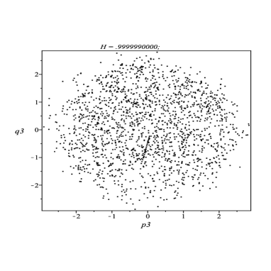
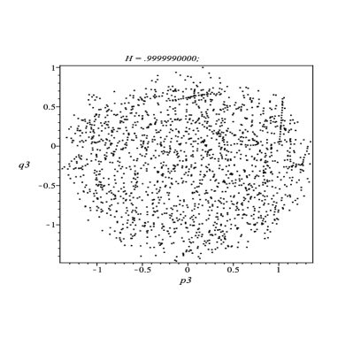
Figure 1: Poincaré cross sections for $\beta/(\sqrt{2}\alpha)=-1$ and $\beta/(\sqrt{2}\alpha)=1$.

A meticulous proof would require probably the use of higher variations [15, 16].

A natural question arises: what happens when $\alpha=0,\,\beta\neq 0$? Numerical experiments suggest a very regular behavior of the trajectories of (2). Note that if any additional integral $F$ exists, it should be a real valued combination of the generators (1) of the normal form since $\{H_{2},F\}=0$. After some calculations the function $F$ (1.10) turns out to be the needed additional integral, which justifies (ii). This proves Theorem 1.

$\hfill\blacksquare$

3 Concluding Remark

In this note we study the integrability of the truncated to order four normal form of the 1 : 2 : 2 resonance. This normal form contains too many parameters which makes difficult the complete analysis of the problem. Foe a generic choice of parameters we prove that the corresponding normal form is meromorphically non-integrable. Due to the works [8, 7] the non-integrability has a clear geometric and dynamical meaning. As in the study of other first order resonances [5] we use the Morales-Ramis theory.

Perhaps, the obtaining of two integrable cases is the more interesting result here. The first one (1.7) is natural and easy, moreover, it is KAM non-degenerated upon certain conditions on the parameters. The second one with the extra integral (1.10) is non-trivial and can not be explained by obvious symmetry.

In fact, we could extend the non-integrability result for a larger set of parameters of the normal form, but couldn’t succeed in finding an additional integral, so it is preferable to state Theorem 1 in that way. Of course, this does not mean that there are no other integrable cases.

Let us note that the algebraic approach adopted here and in [5] can be applied to study integrability of other resonance Hamiltonian normal forms in three degrees of freedom. cf. [22, 13]. We can remove the quadratic part of the normal form $H_{2}$ one way or another. This allows us to deal with the resonances $1:k:l$ even in the case when $k$ ( or $l$) is negative. A systematic way how to obtain the generators of the corresponding normal forms is given in Hansmann [13]. Note that 1 : 2 : -2 and 1 : -1 : 2 are generically non semi-simple.

Acknowledgements.

This work is supported by grant DN 02-5 of Bulgarian Fund ”Scientific Research”.

References

• [1] E. van der Aa, First order resonances in three degrees of freedom, Celest. Mech. 31 (1983) 163–191.
• [2] E. van der Aa, F. Verhulst, Asymptotic integrability and periodic solutions of a Hamiltonian system in 1 : 2 : 2 resonance, SIAM J. Math. Anal. 15(5)(1984) 890–911.
• [3] V. Arnold, V. Kozlov, and A. Neishtadt, Mathematical Aspects of Classical and Celestial Mechanics, in: Dynamical systems III, Springer-Verlag, New York 2006.
• [4] W. Balser, W. Jurkat, D. Lutz, Birkhoff invariants and Stokes’ multipliers for meromorphic linear differntial equations, J. Math. Anal. Appl. 71 (1979) 48–94.
• [5] O. Christov, Non-integrability of first order resonances in Hamiltonian systems in three degrees of freedom, Celest. Mech. Dyn. Astr. 112 (2012) 149–167.
• [6] J. Ford, The statistical mechanics of classical analytic dynamics, in: Cohen, E.D.G. (ed.) Fundamental Problems in Statistical Mechanics, vol. 3. 1975.
• [7] G. Haller, Chaos near Resonance, App. Math. Sciences, vol. 138, Springer-Verlag, New York 1999.
• [8] G. Haller, S. Wiggins, Geometry and chaos near resonant equilibria of 3-DOF Hamiltonian systems, Phys. D 90 (1996) 319–365.
• [9] M. Kummer, On resonant Hamiltonian systems with finitely many degrees of freedom, p. 19–31 in: A. SΓ‘enz, et al. (Eds.), Local and global methods of nonlinear dynamics, Silver Spring 1984, Lecture Notes in Physiscs, vol. 252, Springer-Verlag, Berlin 1986.
• [10] A. Magid, Lectures on Differential Galois Theory, University lecture series, vol. 7, AMS, Providence, 1994.
• [11] J. Martinet, J-P. Ramis, ThΓ©orie de Galois diffΓ©rentielle et resommation, Computer algebra and Differntial equations, Academic Press, London, 117–214 (1989).
• [12] C. Mitschi, Differential Galois groups and G-functions, Computer algebra and Differential equations, Academic Press, London, 149–180 (1991).
• [13] H. Hansmann, Local and Semi-Local Bifurcations in Hamiltonian Dynamical Systems: Results and Examples, Lecture Notes in Mathematics, vol. 1893, Springer, Berlin, 2007.
• [14] J. Morales Ruiz, Differential Galois Theory and Non integrability of Hamiltonian Systems, Prog. in Math., v. 179, BirkhΓ€user, 1999.
• [15] J. Morales-Ruiz, J-P. Ramis, and C. SimΓ³, Integrability of Hamiltonian systems and differential Galois groups of higher variational equations, Annales scientifiques de l’École normale supΓ©rieure 40 (2007) 845–884.
• [16] J. Morales-Ruiz, J-P. Ramis, Integrability of Dynamical systems through Differential Galois Theory: practical guide, Contemporary Math. 509 (2010).
• [17] B. Rink, Symmetry and resonance in periodic FPU-chains, Comm. Math. Phys. 218 (3)(2001), 665–685.
• [18] M. van der Put, M. Singer, Galois Theory of Linear Differential Equations, Grundlehren der Mathematischen Wissenschaften, vol. 328, Springer-Verlag, 2003.
• [19] J. Sanders, F. Verhulst, J. Murdock, Averaging methods in Nonlinear Dynamical Systems, Appl. Math. Sci., vol. 59, Springer-Verlag 2007.
• [20] M. Singer, Introduction to the Galois theory of linear differential equations, Algebraic theory of differential equations, London Mathematical Society Lecture Note Series, Cambridge University Press, Vol. 2, No. 357, 1–82, 2009.
• [21] F. Verhulst, Symmetry and integrability in Hamiltonian normal forms, in: D. Bambusi, G. Gaeta (Eds.), Symmetry and Perturbation Theory, Quadern GNFM, Farenze, 245–284, 1998.
• [22] F. Verhulst, Integrability and non-integrability of Hamiltonian normal forms, Acta Appl. Math. 137 (2015) 253–272.
• [23] S. Ziglin, Branching of solutions and non-existence of first integrals in Hamiltonian mechanics, Func. Anal. Appl., I – vol. 16, (1982) 30–41; II – vol. 17, 1983 8–23.