Backlash Identification in Two-Mass Systems by Delayed Relay Feedback

Abstract

Backlash, also known as mechanical play, is a piecewise differentiable nonlinearity which exists in several actuated systems, comprising, e.g., rack-and-pinion drives, shaft couplings, toothed gears, and other machine elements. Generally, the backlash is nested between the moving parts of a complex dynamic system, which handicaps its proper detection and identification. A classical example is the two-mass system which can approximate numerous mechanisms connected by a shaft (or link) with relatively high stiffness and backlash in series. Information about the presence and extent of the backlash is seldom exactly known and is rather conditional upon factors such as wear, fatigue and incipient failures in the components. This paper proposes a novel backlash identification method using one-side sensing of a two-mass system. The method is based on the delayed relay operator in feedback that allows stable and controllable limit cycles to be induced and operated within the (unknown) backlash gap. The system model, with structural transformations required for the one-side backlash measurements, is given, along with the analysis of the delayed relay in velocity feedback. Experimental evaluations are shown for a two-inertia motor bench that has coupling with backlash gap of about one degree.

1 Introduction

Mechanical backlash, i.e., the phenomenon of play between adjacent movable parts, is well known and causes rather disturbing side-effects such as lost motion, undesired limit cycles in a closed control loop, reduction of the apparent natural frequencies and other. For a review of this phenomenon we refer to [1]. It is the progressive wear and fatigue-related cracks in mechanical structures that can develop over the operation time of an actuated system with backlash; this is in addition to appearance of a parasitic noise [2]. Moreover, increasing backlash leads to more strongly pronounced chaotic behavior [3] that, in general, mitigates against accurate motion control of the system.

Two-mass systems with backlash, as schematically shown in Fig. 1, constitute a rather large class of the motion systems. Here, a driving member, which is a motor or generally actuator, is coupled to the driven member (load) by various construction elements, i.e., gears, couplings, or kinematic pairs. The connecting elements contain a finite gap, here denoted by $2\beta$, usually of a small size comparing to the rated relative displacement of the motion system. Within this gap, both moving masses become decoupled from each other. It is important to note that this structure has a backlash in feedback which differs significantly from feedthrough systems where a static backlash element appears either in the input or output channel. Those types of systems with backlash have also attracted considerable attention in systems analysis and control, see, e.g., [4], [5]. However, they should not be confused with the types of backlash feedback systems as depicted in Fig. 1 and addressed in the following. Some previous studies which consider analysis and control of backlash feedback systems can be found in, e.g., [6, 7, 8].

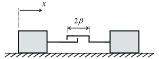
Figure 1: Two-mass system with backlash.

Despite the fact that the fundamental understanding of backlash mechanisms appears to be something of a solved problem, case-specific modeling, and above all, reliable detection and identification still remain relevant and open-ended problems in systems and control engineering. Applications can be found in industrial robotic manipulators, e.g., [9], flexible medical robots, e.g., [10], servo drive systems, e.g., [11, 12], automotive power trains, e.g., [13] and other areas. Information about the presence and extent of backlash, which is a rather undesirable structural element, is seldom exactly known, and usually requires identification under regular operational conditions, i.e. during exploitation. When both the motor-side and load-side of a two-mass (two-inertia) system are equipped with high-resolution position sensors (encoders), see for instance [14], the identification of backlash becomes a trivial task which can be accomplished under various quasi-static, low-excitation conditions. A frequently encountered case, however, is when load-side sensing is not available, or is associated with special auxiliary measures which can markedly differ from the normal operational conditions. A typical situation occurs when only the driving actuator is equipped with an encoder or other position-giving sensor, while the total drive train, presumably with backlash, has no access to additional measurements.

In the last two decades, various strategies for estimation, and hence identification, of the backlash between two moving parts, have been developed. A very early study and analysis of the backlash phenomenon in geared mechanisms was made by [15]. A specially designed impulse excitation and motor current filtering method was proposed in [11] for high-precision servo systems. While straightforward in realization, the method relies on the assumption that the torque impulses are sufficient to move the motor and, at the same time, to keep the load immobile. For systems with high and uncertain damping and additional elasticity modes, such excitation can be challenging with regard to realization and manifestation of the backlash. The nonlinear observation of backlash states was proposed and evaluated in [16], though both motor-side and load-side measurements were required. An identification approach based on the ridges and skeletons of wavelet transforms was demonstrated by [17]. The method requires a relatively broadband frequency excitation and a combined time-frequency analysis that can be challenging in a practical application. One of the most established strategies of backlash identification, using motor-side sensing only, was reported in [12]. It should be noted, however, that the underlying ideas were previously provided in [15]. This approach will also be taken as a reference method for experimental evaluation in the present work. Another, more frequency-domain-related approach for analyzing backlash by approximating it with a describing function, can be found in [18]. This relies on the so-called ”exact backlash mode” introduced in [19]. Describing function analysis of systems with impact and backlash can be found in [20]. An experimental comparison of several backlash identification methods, mainly based on the previous works of [11, 13, 12], can be found in [21]. There, the authors concluded that the method of integration of the motor speed [12] was the most accurate from those under evaluation.

The objective of this paper is to introduce a new strategy for identifying the backlash in two-mass systems when only a motor-side sensing is available. In addition, this method does not require a large excitation of the overall motion dynamics, in contrast to [12]. This can be advantageous for various machines and mechanisms where the load cannot be driven at higher velocities and accelerations. The proposed method relies on the appearance of stable and controllable limit cycles, while using a delayed relay in the velocity feedback loop. We recall that relay feedback systems have been intensively studied since the earlier pioneering works [22, 23] and successfully applied in, e.g., auto-tuning of controllers [24] and other purposes such as mass identification [25]. In the present study, the uncertainties and parasitic effects of the system dynamics are not explicitly taken into account, but the relay in feedback provides the necessary robustification, which is also confirmed by experiments. Further we note that attempts to use a relay feedback for identifying backlash in two-mass systems were also made in [26]. However, the relay feedback was solely used for inducing a large-amplitude periodic motion, while the underlying identification strategy relied on the motor speed pattern analysis, similar as in [12]. Furthermore, an exact detection of zero-crossing and extremum instants is required, along with the ratio of the masses (correspondingly inertias).

The rest of the paper is organized as follows. In section II we describe the underlying modeling approach for two-mass systems with backlash, and the required structural transformations which allow consideration of the two-mass system as a plant with the motor-side sensing only. Section III contains a detailed analysis of the feedback relay system and induced limit cycles, including controllable drifting, which enables operating the motor within and beyond the backlash gap. An experimental case study with the minimal necessary identification of system parameters and relay-based backlash identification is provided in section IV, together with comparison to the reference method reported in [12]. The paper is summarized and the conclusions are drawn in section V.

2 Two-Mass System with Backlash

The block diagram of a generalized two-mass system with backlash is shown in Fig. 2. Note that this complies with the principal structure introduced in section 1, cf. with Fig. 1. The motor-side and load-side dynamics, described in the relative coordinates $x_{m}$ and $x_{L}$ respectively, are given by

$$m\ddot{x}_{m}+d\dot{x}_{m}+f\mathrm{sign}(\dot{x}_{m})=u-\tau,$$ (1)

$$M\ddot{x}_{L}+D\dot{x}_{L}+F\mathrm{sign}(\dot{x}_{L})=\tau.$$ (2)

Both are coupled in the forward and feedback manner by the overall transmitted force $\tau$, which is often referred to as a link (or joint) force. Note that in the following we will use the single terms force, displacement and velocity while keeping in mind the generalized forces, correspondingly generalized motion variables. Thus, the rotary coordinates and corresponding rotary degrees of freedom will be equally considered without changing the notation of the introduced variables. For example, in the case study of the two-inertia system presented in section 4. Clearly, the parameters $m$, $M$, $d$, $D$, $f$ and $F$ are the motor and load masses, damping and Coulomb friction coefficients respectively. We will also denote the known invertible mapping $(u-\tau)\mapsto x_{m}$ by $G_{m}$ and $\tau\mapsto x_{L}$ by $G_{L}$. Here, we explicitly avoid any notations of the transfer function since the dynamics of (1) and (2) include also the nonlinear terms of Coulomb friction. Furthermore we note that despite nonlinear friction can impose more complex by-effects, see e.g. [27, 28], a constant Coulomb friction only is considered here. This is justified by using the discontinuous relay operator in feedback which allows overcoming stiction and other transient by-effects of the nonlinear friction. Using the nonlinear function $g(\cdot)$, where the parameters are unknown but a certain structure can be assumed, we will elucidate the force transmission characteristics of the link.

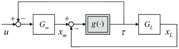
Figure 2: Block diagram of two-mass system with backlash in the link.

Usually the link is excited by the relative displacement, directly resulting from

$$\delta=x_{m}-x_{L},$$ (3)

between the motor and load. We assume that the link transfer characteristics offer a relatively high, but yet finite, stiffness and incorporate a backlash connected in series. Under high stiffness conditions we understand the first resonance peak which can be detected and identified within the measurable frequency range, however sufficiently beyond the input frequencies and control bandwidth of the system.

We assume that the backlash itself is sufficiently damped so that the relative displacement between the ”impact pair” is not subject to any long-term oscillations when the mechanics engage. Here, we recall that the simplest modeling approach for the backlash in two-mass systems, used for instance in [12, 14], applies the dead-zone operator (with $\delta$ argument) only, while the dead-zone output is subsequently gained by the stiffness of the link. This arrangement results in a proper backlash behavior merely at lower frequencies, but tends to produce spurious $\delta$-oscillations at higher harmonics. More detailed consideration of the backlash in two-mass systems incorporates a nonlinear damping at impact [8], for which advanced impact models can be found, e.g., in [29, 30]. Also note that in [19], an inelastic impact was considered when the backlash gap was closed, and the switching distinction for gap and contact modes was made, cf. further with eq. (4).

The above assumption of sufficient backlash damping allows a simple structural transformation of the block diagram from Fig. 2 to be made. Assuming a rigid coupling at the backlash contacts and loss-of-force transmission at the backlash gap, an equivalent model can be obtained, as shown in Fig. 3. Obviously, the consideration of the backlash element in Fig. 3 is purely kinematic, so that an ideal play-type hysteresis [31, 32] is assumed between the motor and load displacements. The kinematic backlash, which is the Prandtl-Ishlinskii operator of the play type, can be written in the differential form as

$$\dot{x}_{L}=\left\{\begin{array}[]{ll}\dot{x}_{m}&\hbox{if }\;x_{L}=x_{m}-\beta,\;\dot{x}_{m}>0\>,\\[2.84544pt] \dot{x}_{m}&\hbox{if }\;x_{L}=x_{m}+\beta,\;\dot{x}_{m}<0\>,\\[2.84544pt] 0&\hbox{if }\;x_{m}-\beta<x_{L}<x_{m}+\beta\>,\\[2.84544pt] 0&\hbox{otherwise}\>,\end{array}\right.$$ (4)

cf. with [9, 33], where the total gap is $2\beta$. Note that the backlash acts as a structure-switching nonlinearity $x_{L}=\mathrm{P}[x_{m}]$, so that two operational modes are distinguished. The first mode, within the backlash gap i.e. when $|\delta|<\beta$, implies zero feedback of the $G_{L}^{-1}$ dynamics. The second mode, is during mechanics engagement, i.e., $|\delta|=\beta$ provides the feedback coupling by $G_{L}^{-1}$, so that the system performs as a single mass with the lumped parameters $(m+M)$ and $(d+D)$. During the switching between both modes the play operator (4) becomes non-differentiable. That is, the first time-derivative of the $\mathrm{P}$-output to an inherently $\mathcal{C}^{2}$-smooth motor position input contains step discontinuities. Correspondingly, the second time-derivative constitutes the weighted delta impulses, in terms of the distribution theory. These impulses can be interpreted as an instantaneous impact force $\tau$ which excites the motor dynamics when the backlash switches between gap and engagement, and vice versa. We should stress that this switching mechanism does not explicitly account for the link stiffness and damping at impact, as previously mentioned. However, this is not critical at lower frequencies, since the link stiffness is assumed to be sufficiently high, and the motor and load dynamics are subject to the viscous and Coulomb friction damping; cf. (1) and (2). Also we note that the hybrid approach, with a switching structure for the gap and engagement, was also used in [34] for modeling and control of mechanical systems with backlash.

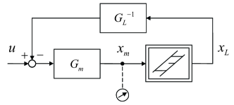
Figure 3: Equivalent block diagram for modeling the two-mass system with backlash described by the play-type hysteresis operator.

A significant feature of the equivalent model shown in Fig. 3 is that it allows the two-mass system with backlash to be considered as a single closed loop, while assuming that the motor-side sensing only is available. This is a decisive property we will make use of when identifying backlash by using one-side sensing of the two-mass system. It is to recall that the loop is closed during the engagement mode and open during the gap mode of the backlash in dynamic system. This results in an impulsive behavior during mode switching. Therefore, the motor dynamics are disturbed periodically when a controllable stable limit cycle occurs. We analyze this situation further in section 3.3.

3 Delayed Relay Feedback

The proposed backlash identification is based on the delayed relay in the feedback of the motor velocity. Consider the relay feedback system as shown in Fig. 4. Note that the structure represents our system, as introduced in section 2, when operating in the backlash gap mode, i.e., $y=0$. From the point of view of a control loop with relay, the switching feedback force (see Fig. 3) can be seen as an exogenous signal $y$. The non-ideal relay, also known as hysteron [31], switches between two output values $\pm h$, while the switching input is ”delayed” by the predefined threshold values $\pm e$. Therefore $2e$ is the relay width, corresponding to the hysteron’s size, and $h$ is the amplification gain of the relay output. The hysteron with input $z$ is defined, according to [27], as:

$$H(t)=h\,\min\Bigl{[}\mathrm{sign}(z+e),\max\bigl{[}H(t^{-}),\mathrm{sign}(z-e)\bigr{]}\Bigr{]},$$ (5)

while its initial state at $t_{0}$ is given by

$$H(t_{0})=\left\{\begin{array}[]{ll}h\,\mathrm{sign}\bigl{(}z(t_{0})\bigr{)},&\hbox{ if }z(t_{0})\in(-\infty,-e]\,\vee\,[e,\infty),\\[2.84544pt] \left\{-h,+h\right\},&\hbox{ otherwise.}\end{array}\right.$$ (6)

It can be seen that the hysteron has a memory of the previous state at $t^{-}$ and keeps its value as long as $z\in(-e,e)$.

In the following, we will first assume that the relay feedback system from Fig. 4 is self-sustaining, i.e., without a disturbing factor, i.e., $y=0$. Subsequently, in sections 3.2 and 3.3 we will allow for $y\neq 0$ and analyze the resulting behavior while approaching the proposed strategy of backlash identification. Note that $y\neq 0$ corresponds to the engagement mode of the backlash, with reference to the original system from Fig. 3.

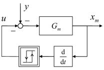
Figure 4: Relay feedback system with motor dynamics in the loop.

3.1 Symmetric Unimodal Stable Limit Cycle

It is well known that relay feedback systems can possess a stable limit cycle [35]. For a single-input-single-output (SISO) linear time invariant (LTI) system we write

$$\dot{x} = Ax+Bu,$$ (7)

$$z = Cx,$$ (8)

assuming the $n\times n$ system matrix $A$ is a Hurwitz matrix, and assuming that the input and output coupling vectors $B$ and $C$ satisfy $CB>0$. When a relay $u=-H[z]$ closes the feedback loop, the state space obtains two parallel switching surfaces which partition the state space into the corresponding cells. For $H>0$, the system dynamics is given by $\dot{x}=Ax-Bh$, and for $H<0$ by $\dot{x}=Ax+Bh$, while the total amplitude of the relay switching is $2h$, see (5). If the relay in (5) is non-ideal, i.e., $e>0$, then the existence of a solution of (7) and (8) with relay (5) in feedback is guaranteed [36], and the state trajectory will reach one of the switching surfaces for an arbitrary initial state. The necessary condition for globally stable limit cycles of the relay feedback system with a relay gain $h$, is given by

$$CA^{-1}Bh+e<0,$$ (9)

cf. with [36]. Otherwise, a trajectory starting at $A^{-1}BH$ would not converge to the limit cycle. In the following, we describe the most significant characteristics of the stable limit cycles of the relay feedback system as shown in Fig. 4. Note that these base on the above assumptions and conditions taken from the literature. For more details on the existence and analysis of limit cycles in relay feedback systems we refer to [35, 37, 36]. The limit cycle existence condition in the control systems with backlash and friction has also been studied in [38].

Considering the motor velocity dynamics (1), first without Coulomb friction, and the relay (5) in negative feedback, the condition for stable limit cycles (9) becomes

$$e<\frac{h}{d}.$$ (10)

In fact, the velocity threshold $|e|$ should be first reachable for a given system damping and excitation force provided during the last switching of the relay. Therefore, (10) specifies the boundaries for parameterization of the relay, so that to ensure the trajectory reaches one of the switching surfaces $\pm e$ independently of the initial state. In cases where the motor damping is not well known, its upper bound can be assumed, thus capturing the ”worst case” of an overdamped system.

Once also the Coulomb friction contributes in (1), the condition (10) becomes a necessary but not a sufficient one. Obviously, sufficient conditions should relate the motor Coulomb friction coefficient $f$ to the relay, as in (5), since both are the matched operators of one and the same argument $\dot{x}_{m}$. Both are discrete switching operators, so that

$$h>f$$ (11)

is required for the relay to overcome the Coulomb friction. It is essential that the velocity sign changes while the (delayed) relay simultaneously keeps its control value. For the boundary case $f<h\rightarrow f$, the relay feedback system with, for instance, $H<0$ becomes $m\ddot{x}_{m}=-d\dot{x}_{m}+2f$ after the velocity sign changes from the positive to negative. Based on that, the condition for the relay threshold results in

$$e<\frac{2f}{d},$$ (12)

while following the same line of development as that for deriving (10) from (9). Note that all three conditions (10)-(12) should hold, in order to guarantee the existence of a stable limit cycle once the Coulomb friction is incorporated.

For determining the position amplitude of the limit cycles, whose velocity amplitude is $2e$ by definition, consider the state trajectories of the system $m\ddot{x}_{m}+d\dot{x}_{m}+f\mathrm{sign}(\dot{x}_{m})=-h$. The corresponding initial velocity is $e$, immediately after the relay switches down to $-h$. It can easily be shown that the associated phase portrait of the state trajectories, with an initial position $x_{m}(0)$, can be written as

$$x_{m}=\frac{-0.5m\dot{x}_{m}^{2}}{d\dot{x}_{m}+h+f\mathrm{sign}(\dot{x}_{m})}+x_{m}(0).$$ (13)

Solving (13) for three characteristic velocities $\dot{x}_{m}=\{e,0,-e\}$, one obtains the start, maximal, and minimal positions $x3$, $x4$, and $x2$ of the half-limit cycle, as shown in Fig. 5.

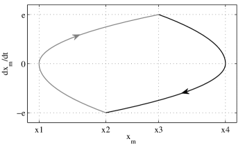
Figure 5: Symmetric unimodal limit cycle.

Note that in the case of $d,f=0$, the points $x2$ and $x3$ coincide with each other. Since the symmetric relay (5) induces a symmetric unimodal limit cycle, the second half-cycle can be obtained by mirroring the first one, derived by (13); once across the axis connecting both switching points at $\pm e$ and once across the orthogonal axis going through its center (see Fig. 5). The intersection of the axes constitutes the origin of the limit cycles, which is the manifold $\{x_{m},|\,\dot{x}_{m}=0\}$. Obviously, the $x_{m}$ coordinate depends on the initial conditions and the system excitation. We also recall that the limit cycle is symmetric if $\xi(t+t^{*})=-\xi(t)$ where $\xi(t)$ is a nontrivial periodic solution of (5)-(8) with period $2t^{\ast}$. The limit cycle is also called unimodal when it switches only twice per period; see [36] for details. The symmetry and unimodality of the limit cycle, as depicted in Fig. 5, implies that $x4-x3=x2-x1$. Therefore the total position amplitude, denoted by $X_{\xi}$, becomes $2(x4-x3)+(x3-x2)$. Evaluating $x2$, $x3$, $x4$ points, computed by (13), yields

$$X_{\xi}=-\frac{e^{2}h\,m}{(f+h+d\,e)(f-h+d\,e)}.$$ (14)

For determining the period of the limit cycle, the same differential equation $m\ddot{x}_{m}+d\dot{x}_{m}+f\mathrm{sign}(\dot{x}_{m})=-h$ is solved with respect to time, together with the initial and final values $\dot{x}_{m}(0)=e$ and $\dot{x}_{m}(t^{*})=-e$ respectively. This yields

$$t^{*}=-\frac{m}{d}\Bigl{[}\ln\Bigl{(}1+\frac{d\,e}{f-h}\Bigr{)}+\ln\Bigl{(}\frac{f+h}{f+h+d\,e}\Bigr{)}\Bigr{]}.$$ (15)

3.2 Drifting Limit Cycle

In the previous subsection, the conditions for a unimodal limit cycle of the system as shown in Fig. 4 were derived, and the characteristic features in terms of the displacement amplitude and period were given by (14) and (15). We note that the limit cycle can appear within the gap mode of backlash, (see section II), provided $X_{\xi}<2\beta$, so that the motor and load remain decoupled (compare with Fig. 3).

In order to realize a drifting limit cycle, consider a modified relay from (5) and (6) so that the amplitude becomes

$$h=\left\{\begin{array}[]{ll}\alpha_{+}h_{0},&\hbox{ if }\;\mathrm{sign}(H)>0,\\ \alpha_{-}h_{0},&\hbox{ if }\;\mathrm{sign}(H)<0.\\ \end{array}\right.$$ (16)

Here, $h_{0}$ is the amplitude of the underlying symmetric relay (5) and (6), and $\alpha_{+},\alpha_{-}\geq 1$ with $\alpha_{+}\neq\alpha_{-}$ scales it, so as to provide an unbalanced control effort when switching. This leads to differing acceleration and deceleration phases of the limit cycle, so that the trajectory does not close after one period (compare with Fig. 5), and becomes continuously drifting as in the example shown in Fig. 6. Note that the case where $\alpha_{-}>\alpha_{+}$ is illustrated here. As in section 3.1, one can solve the trajectories between two consecutive switches separately for $\alpha_{-}h_{0}$ and $\alpha_{+}h_{0}$, and obtain the relative shift $X_{C}=x_{e}-x_{s}$ of the limit cycle per period as follows:

$$X_{C}=\frac{-e^{2}h_{0}^{2}\,m(\alpha_{-}^{2}-\alpha_{+}^{2})\,(f+d\,e)}{(-\alpha_{-}^{2}h_{0}^{2}+d^{2}e^{2}+2de+f^{2})(-\alpha_{+}^{2}h_{0}^{2}+d^{2}e^{2}+2de+f^{2})}.$$ (17)

Following the same line of developments as in section 3.1, the period of the drifting limit cycle, i.e., the time of arrival at $x_{e}$ can be obtained as

$$T_{C} = -\frac{m}{d}\Bigl{(}\ln\frac{f+\alpha_{-}h_{0}}{f+de+\alpha_{-}h_{0}}+\ln\frac{f+de-\alpha_{-}h_{0}}{f-\alpha_{-}h_{0}}+$$ (18)

$$+ \ln\frac{f+\alpha_{+}h_{0}}{f+de+\alpha_{+}h_{0}}+\ln\frac{f+de-\alpha_{+}h_{0}}{f-\alpha_{+}h_{0}}\Bigr{)}$$

Obviously, the average drifting velocity of the limit cycle can be computed from (17) and (18) as $\dot{X}_{C}\approx X_{C}/T_{C}$.

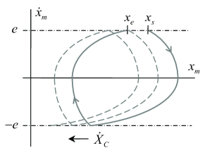
Figure 6: Drifting limit cycle of amplitude-asymmetric relay ($\alpha_{-}>\alpha_{+}$)

Note that (17) and (18) characterize the drifting limit cycle which proceeds within the backlash gap without impact with the load side. The impact behavior of drifting limit cycles is addressed below, and that from the associated relative load displacement point of view.

3.3 Impact Behavior at Limit Cycles

In order to analyze the impact behavior at limit cycles, i.e., the situation where the load side is permanently shifted, as long as it is periodically excited by the drifting limit cycle, consider first the impact phenomenon of two colliding masses $m$ and $M$. Note that when considering the impact and the engagement mode of the backlash, the conditions (10)-(12) are not explicitly re-evaluated due to nontrivial (and also possibly chaotic) solutions. However, making some smooth assumptions, we evaluate the impact behavior at the limit cycles and show their persistence within numerical simulations and later in experiments.

Introducing the coefficient of restitution $0\leq\varepsilon\leq 1$ and denoting the velocities immediately after impact by the superscript ”⁺” one can show that

$$\dot{x}_{m}^{+} = \frac{\dot{x}_{L}(1-\varepsilon)M+\dot{x}_{m}(m-\varepsilon M)}{M+m},$$ (19)

$$\dot{x}_{L}^{+} = \frac{\dot{x}_{L}(M-\varepsilon m)+\dot{x}_{m}(1+\varepsilon)m}{M+m}.$$ (20)

The above velocity jumps directly follow from the Newton’s law and the conservation of momentum, see e.g. [20] for details. Recall that a zero coefficient of restitution means a fully plastic collision, while $\varepsilon=1$ constitutes the ideal elastic case. For the relatively low velocities at impact (since small backlash gaps are usually assumed) and stiff (metallic) backlash structures, we take $\varepsilon\approx 1$, cf. with [29]. Further, we assume the load velocity to be zero and the motor velocity amplitude to be (in the worst case) maximal, i.e., $\max|\dot{x}_{m}|=e$, immediately before the impact. Due to the above assumptions, the load velocity (20) after impact can be determined as an upper bound:

$$\bar{\dot{x}}_{L}^{+}=\frac{2\,m\,e}{M+m}.$$ (21)

Note that (21) constitutes an ideal case without any structural and frictional damping at impact, whereas a real load velocity after impact will generally be lower in amplitude than (21). Nevertheless, (21) provides a reasonable measure of the relative load motion immediately after the backlash engages. Solving the unidirectional motion $M\ddot{x}_{L}+D\dot{x}_{L}+F=0$, which, for zero final velocity and the initial velocity given by (21), yields the relative displacement of the load until the idle state as

$$X_{L}=\frac{F\,M}{D^{2}}\ln\Bigl{(}\frac{F(M+m)}{F(M+m)+2D\,e\,m}\Bigr{)}+\frac{2M\,e\,m}{D(M+m)}.$$ (22)

Intuitively, assuming well-damped (through $F$ and $D$) load dynamics, the load displacement $X_{L}$ due to a single impulse at the impact should be relatively low. At the same time, it can be seen that the logarithmic contribution with negative sign in the first summand of (22) is balanced by the linear increase of the second summand, depending on the parameter $e$. In the sum, the quadratic shape of $X_{L}$ as a function of $e$ occurs at lower values of $e$, and it approaches a linear slope once $e$ grows (see Fig. 7). Hence, the $e$ parameter should be kept as low-valued as possible, given the system parameters $m$, $M$, $D$ and $F$. This will ensure a displacement of the load which is as low as possible, i.e., $X_{L}\rightarrow 0$, induced by the single impulse at impact. Furthermore, low values of $e$ are required firstly to fulfill the necessary and sufficient conditions (10) and (12) of the limit cycle, and secondly to keep the amplitude as low as possible and therefore within the backlash gap (see (14)).

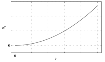
Figure 7: Relative displacement of the load after the backlash impact as a function of the relay parameter $e$ according to (22); qualitative example.

Obviously, the maximal load displacement (22) will be induced periodically by the drifting limit cycle, (see section 3.2), each time the impact occurs. In fact, the motor side, which is moving in a drifting limit cycle, produces a sequence of impulses that continuously ”push” the load side once the instantaneous impulse can overcome the system stiction. The resulting load motion, though periodic due to the drifting limit cycle, can be rather chaotic, due to the amplitude and phase shifts produced by the series of impulses. Due to the inherent uncertainties of the Coulomb friction, viscous damping [39] and non-deterministic system stiction, an exact (analytic) computation of the resulting load motion appears to be only marginally feasible, with unsystematic errors that reveal the predicted trajectory as less credible. At the same time, it can be shown that for the $h$ amplitude selection to be close to $f+F$, a continuous propulsion of the load should occur in the direction of $\dot{X}_{C}$. An example of a numerical simulation of the system (1) and (2) with backlash and an asymmetric relay (5), (6) and (16) in feedback, is shown in Fig. 8. It can be seen that the motor displacement exhibits a uniform drifting limit cycle during the gap mode, until it reaches the backlash boundary and begins to interact with the load side. It is evident that the average drifting velocity of the limit cycle $\dot{X}_{C}$, corresponding to the slope in Fig. 8, differs between the gap and engagement modes. This makes the backlash boundary easily detectable based on the motor displacement trajectory only. Note that in the numerical simulation shown, neither damping uncertainties nor stiction of the load is taken into account. Thus, in a real two-mass system with backlash, a nonuniform motion during engagement mode is expected to differ markedly from that within the backlash gap, cf. with experiments in section 4.

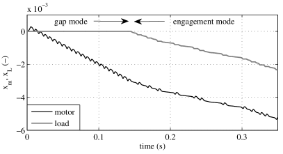
Figure 8: Motor and load displacement during the gap and engagement modes.

4 Experimental Case Study

This section is devoted to an experimental case study on detecting and identifying backlash in a two-inertia system, using only motor-side sensing. The parameters of linear system dynamics, i.e., inertia and damping, are first identified from the frequency response function. The total Coulomb friction level required for the analysis of stable limit cycles (cf. section 3), is estimated using simple unidirectional motion experiments. In addition, the steady limit cycles previously analyzed are induced and confirmed with experiments for unconstrained operation within the backlash gap. The nominal backlash size was measured by means of both motor-side and load-side encoders and used as a reference value. The proposed backlash identification approach, as described in section 3, was followed and evaluated in the laboratory setup. In addition, the reference method [12] was evaluated experimentally for two different excitation conditions and compared with the proposed method.

4.1 Laboratory Setup

An experimental laboratory setup (see picture in Fig. 9), consisting of two identical motors, each with a 20-bit high-resolution encoder, was used in this study.

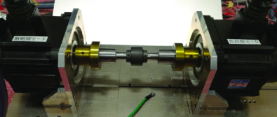
Figure 9: Experimental setup with a gear coupling.

Note that only the motor-side encoder is utilized for the required system identification and for evaluation of the proposed backlash estimation method. The load-side encoder is used for reference measurements only. In this setup, the backlash can be added or removed by replacing the rigid coupling with the gear coupling shown in the picture. A standard proportional-integral (PI) current controller is implemented on-board with the motor amplifier, with a bandwidth of 1.2 kHz. In the experiments, the sampling frequency is set to 2.5 kHz and the control parts are discretized using the Tustin method.

4.2 System Identification

4.2.1 Two-Mass System Parameters

The parameters of the two-mass system, i.e., $m$, $d$, $M$ and $D$, can be identified by measuring the frequency response function (FRF) on the motor side. It is worth emphasizing that the identified motor inertia and damping are sufficient for analyzing and applying the proposed backlash identification approach. Thus, if the above parameters are available or otherwise previously identified, the FRF-based identification discussed below will not be required. The measured frequency characteristics, shown in Fig. 10, disclose the antiresonance and resonance behavior.

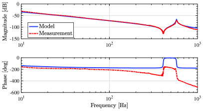
Figure 10: Frequency characteristics measurements of the setup from the motor torque to the motor-side angle versus the fitted two-mass system model.

Table 1: Identified parameters of two-mass system.

Motor-side inertia $m$	8.78e-4	kgm2
Motor-side damping coefficient $d$	6.20e-2	Nms/rad
Load-side inertia $M$	8.78e-4	kgm2
Load-side damping coefficient $D$	3.60e-2	Nms/rad

The parameters of the two-mass (two-inertia) system are identified by fitting both peak regions. Here, the frequency characteristics from the motor torque to the motor-side angle are determined for the setup equipped with rigid coupling (without backlash). This corresponds to the case of a nominal plant where no backlash disturbance develops during the operation. Note that for a sufficient system excitation, similar FRF characteristics can also be obtained in the presence of a small backlash. Otherwise, the basic parameters, such as lumped mass and damping of the motor and load sides, are assumed to be available from the manufacturer’s data sheets and additional data from design correspondingly manufacturing.

The measured FRF shows that the setup can be modeled as a two-mass system which has an antiresonance frequency of about 409 Hz and a resonance frequency of about 583 Hz. The fitted model response is indicated in Fig. 10 by the blue solid line, while the measurement results are indicated by the red dashed line. A visible discrepancy in the phase response is due to an inherent time delay in the digital control system. However, this becomes significant in a higher frequency range only and is therefore neglected. The identified parameters are listed in Table 1.

4.2.2 Coulomb Friction

The combined motor-side and load-side Coulomb friction $f+F$ is identified by measuring the motor torque when the motor-side velocity is controlled for constant reference values. Figure 11 shows the obtained torque-velocity measurements. Blue circles indicate the measured data, captured from multiple constant velocity drive experiments, and the red line indicates the linear slope fitted by the least-squares method. Here, the Coulomb friction torque of 0.1 Nm is determined from the intercept of the fitted line with the torque axis. In the same way, the friction-velocity curve is determined for the negative velocity range, not shown here due to its similarity. Here, the determined Coulomb friction value was $-0.0993$ Nm which demonstrates that the friction behavior of the total drive is sufficiently symmetrical around zero. An average value of $f+F=0.0999$ Nm is further assumed, while a very rough estimation of the motor-side Coulomb friction is half of the total value, i.e., $f\approx 0.05$ Nm. Note that an exact knowledge of $f$ is not required to satisfy the conditions derived in section 3. Knowledge of the total Coulomb friction coefficient $f+F$ alone is sufficient for applying the relay feedback system.

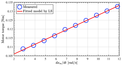
Figure 11: Friction-velocity identification measurements.

4.2.3 Nominal Backlash Size

For evaluation of the proposed method, the nominal backlash size is first identified using both the motor- and load-side encoders. Figure 12 shows the measured $(x_{m}$, $x_{L})$ map when the motor-side position is open-loop controlled by a low-amplitude and low-frequency sinusoidal wave. The detected backlash is $2\beta=19.05$ mrad, which can be seen as a low value, i.e., below one degree.

It should be emphasized that when the motor is moving forwards after a negative direction reversal, the load side is first moving together with the motor side, even though both are within the backlash gap (see the lower left-hand range in Fig. 12).

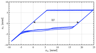
Figure 12: Nominal backlash identified using both encoders.

This spurious side-effect can be explained by adhesion between the motor and load sides and the specific structure of the gear coupling. Since the gear coupling used in the setup consists of an internal tooth ring and two external tooth gears, it exhibits, so to speak, a double backlash, which cannot be exactly captured by the standard modeling assumptions previously made for a two-mass system with backlash. It is evident that the forward transitions, as depicted in Fig. 12 and further in Fig. 16 and Fig. 17, exhibit some non-deterministic creep-like behavior that cannot be attributed to backlash nonlinearity as assumed. Therefore, in order to be able to consider the backlash effect without adhesive disturbances, only the backward-moving phases are regarded as suitable for evaluation.

4.3 Steady Limit Cycle

As described in section 3.1, the delayed relay feedback produces steady limit cycles. The experimentally measured limit cycle is shown in Fig. 13.

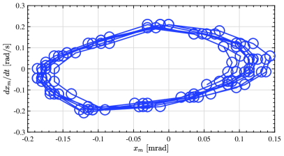
Figure 13: Steady limit cycle caused by delayed relay feedback.

The assumed relay parameters $h=0.1$ and $e=0.1$ satisfy (10)-(12). The total amplitude $X_{\xi}$ of the limit cycle is required to be small compared to the backlash size. In addition, the period of the limit cycle $2t^{*}$ is required to be large enough, with respect to the system sampling rate, so as to ensure a sufficient number of samples per period of the limit cycle. The values computed according to (14) and (15) are $X_{\xi}=0.128$ mrad and $t^{*}=2.45$ msec respectively. The average $X_{\xi}$ value, determined from the example measurements shown in Fig. 13, is about 0.28 mrad. This is not surprising, since the measured steady limit cycle is subject to the time delay of the control system so that the actual switchings do not occur exactly at $\pm e=\pm 0.1$ rad/sec as required by the relay parameterization. Rather, they appear at $\pm 0.2$ rad/sec, which is double the set relay parameter value $e$. Nevertheless, the limit cycle remains stable, almost without drifting, and displays the expected characteristic shape, cf. with Fig. 5. Here, we note that the gear coupling with backlash was installed, so that the steady limit cycle as shown in Fig. 13 clearly occurs within the backlash gap, without impact with the load side. The half-period $t^{*}$, determined from the measurements, corresponds to about six or seven samplings, i.e., 2.4 to 2.8 msec, and is in accordance with that computed by (15). Recall that knowledge of $t^{*}$ is significant for deciding the sufficiency of the sampling rate with regard to the relay control parameters.

4.4 Motor-Side Backlash Identification

The proposed backlash identification method is implemented and evaluated experimentally. The results are evaluated for two different sets of relay parameters. The two cases are defined as follows. Case 1: $h_{0}$=0.12, $e$=0.1, $\alpha$ = 2, and Case 2: $h_{0}$=0.1, $e$=0.1, $\alpha$ = 2.5. The $\alpha$ values are selected by trial and error when operating the feedback relay system and observing sufficient movement (drift) of the resulting limit cycle, cf. with Fig. 8. Note that a periodic sequence for which the relay asymmetry coefficients $\alpha_{+}$ and $\alpha_{-}$ alternate, for example: $[\alpha_{+},\alpha_{-}]$ = [2, 1] for the first five seconds followed by $[\alpha_{+},\alpha_{-}]$ = [1, 2] for the next five seconds, and so on, has been applied.

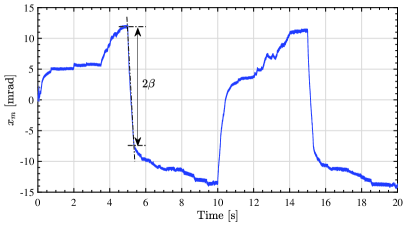
Figure 14: Backlash identification using the proposed method, Case 1.

This allows for changing the drift direction of the limit cycles, and therefore exploring both the backlash gap in both directions as well as the coupled motion beyond the gap, i.e., during the engagement mode. Recall that only the backward-moving phases are evaluated so as to estimate the backlash without adhesion side-effects.

The motor position responses in Case 1 and Case 2 are shown in Fig. 14 and Fig. 15 respectively.

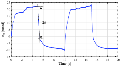
Figure 15: Backlash identification using the proposed method, Case 2.

The full backlash width 2$\beta$ can be determined by the sudden change of the motor position’s slope. The slope of the motor position is steeply and uniform within the backlash gap, since the load is decoupled from the motor side. When the impact between them occurs, the slope suddenly changes and becomes less steep and also irregular. The determined 2$\beta$ values in Case 1 and Case 2 are 19.30 mrad and 23.62 mrad respectively, while the nominal backlash width identified using the load-side encoder, as in section 4.2, is 19.05 mrad. This confirms that the proposed method can identify the backlash width using the motor-side information only. Note that the recorded motor position pattern is subject to various deviations between the slopes over multiple periods which mitigates against an exact read-off of the backlash size value (see Fig. 14 and Fig. 15). For accuracy enhancement and correspondingly better generalization, the $2\beta$ values read-off over multiple periods can be averaged.

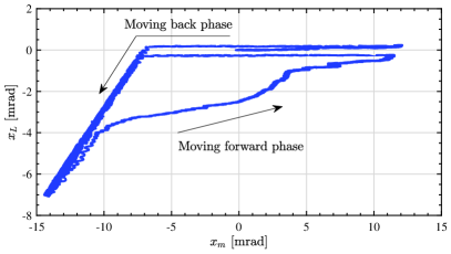
Figure 16: Measured $x_{L}$-$x_{m}$ map in Case 1.

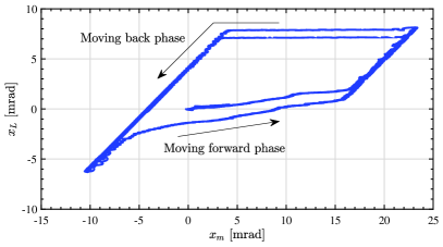
Figure 17: Measured $x_{L}$-$x_{m}$ map in Case 2.

Figures 16 and 17 show the corresponding $(x_{m},x_{L})$ maps, as a reference measurement, for both experimental cases. Recall that the load-side encoder signal is not used for backlash identification. Both figures indicate that the limit cycles generated by the delayed relay with asymmetric amplitudes are drifting controllably along all transitions of the backlash. Only the forward-moving phases suffer from adhesion side-effects, while the backwards phases coincide exactly with the backlash shape, cf. with Fig. 12.

4.5 Comparison with Reference Method

In order to assess the performance of the proposed method, another already established backlash identification strategy [12] has been taken as a reference method. This method also uses the motor-side information only when identifying the backlash in two-inertia systems. The basics of the reference method are described below. For more details we refer to [15, 12].

The reference method applies the triangular-wave reference velocity to the PI motor velocity controller. Considering the controlled plant as a one-inertia system, i.e., with the lumped parameters $m+M$ and $d+D$, the PI velocity controller has been designed by the pole placement such that its control bandwidth is set to 5 Hz. After the sign of the motor-side acceleration changes, due to the triangular velocity reference, the motor side moves back from one end to the opposite end of the backlash gap. At the same time, the load side continues to (freely) move in the initial direction until the backlash impact. The instant when the motor and load sides are decoupled is defined as $t_{1}$ and the instant when the motor and load sides are in contact again is defined as $t_{2}$ (see Fig. 18 and Fig. 19). The reference method identifies the backlash width by integrating the relative motor velocity between these two instants. If the load-side viscosity is small enough, and $t_{2}-t_{1}$ is short enough, the decrease of the load-side velocity during $t_{2}-t_{1}$ can be neglected. Therefore, one can assume $\dot{x}_{L}(t)=\hat{\dot{x}}_{L}=\dot{x}_{m}(t_{1})$ for $t_{1}\leq t\leq t_{2}$. Then, the total backlash width is estimated as

$$2\beta=\left|\int\limits_{t_{1}}^{t_{2}}\bigl{(}\dot{x}_{L}(t)-\dot{x}_{m}(t)\bigr{)}\mathrm{d}t\right|\simeq T_{s}\left|\sum\limits_{k_{1}}^{k_{2}}\bigl{(}\hat{\dot{x}}_{L}-\dot{x}_{m}(k)\bigr{)}\right|,$$ (23)

where $T_{s}$ is the sampling time and $k_{1}t=t_{1}$ and $k_{2}t=t_{2}$.

The results from two different triangular waves are evaluated. Here, two cases are defined as Case 3 – for which the triangular wave slope is 1400 and the period is 0.2 s, and Case 4 – for which the triangular wave slope is 500 and the period is 0.4 s. Obviously, Case 3 is more ”aggressive” in terms of the system excitation, as regards the higher reference acceleration/deceleration of the total drive. Figures 18 and 19 show the measured velocity responses of Case 3 and Case 4 respectively. Since the acceleration in Case 3 is larger than that in Case 4, the decrease in $\dot{x}_{L}(t)$ for $t_{1}\leq t\leq t_{2}$ is smaller, which reduces the estimation error. According to (23), the 2$\beta$ values are calculated as 31.0 mrad and 42.6 mrad for Case 3 and Case 4 respectively.

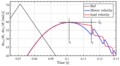
Figure 18: Backlash identification using the reference method, Case 3.

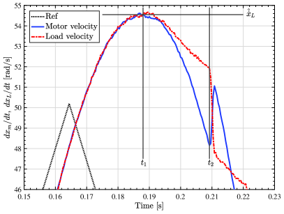
Figure 19: Backlash identification using the reference method, Case 4.

Inherently, the reference method provides an overestimated backlash width, as is apparent from Fig. 18 and Fig. 19. In order to reduce the estimation error, which is mainly driven by the assumption $\dot{x}_{L}(t)=\hat{\dot{x}}_{L}=\dot{x}_{m}(t_{1})$, the reference method requires larger accelerations, to make the decoupling between the motor-side and load-side faster once the sign of the motor acceleration changes. Therefore, the reference method inherently requires more ”aggressive” system excitations and generally larger load inertias to allow for a free, correspondingly decoupled, load motion phase. At the same time, higher and uncertain damping and Coulomb friction values will lead to higher errors when estimating $2\beta$ according to (23).

The backlash identification results for all four above cases, i.e. for the proposed method and reference method, are summarized in Table 2, while the nominal backlash size was measured as 19.05 mrad.

Table 2: Backlash identification results summary

Case 1	Case 2	Case 3	Case 4
19.3 mrad	23.6 mrad	31.0 mrad	42.6 mrad

5 Conclusions

A new approach for identifying backlash in two-mass systems is proposed, with the principal advantage of using the motor-side sensing only, which is a common practice for various machines and mechanisms. The method is based on the delayed relay in feedback of the motor velocity, which allows for inducing the stable limit cycles of amplitudes significantly lower than the backlash gap. The limit cycles can then be operated as drifting while being controlled by an asymmetric relay amplitude. The analyzed period of limit cycles, cf. (15), imposes certain boundary on applicability of the method and that in relation to the sampling time and possible time delays of sensing and actuating in the relay feedback loop. Another factor inherently limiting the proposed method is the sensing resolution of the motor-side, correspondingly the accuracy with which the relative velocity used for relay feedback can be measured.

We provide a detailed analysis of steady and drifting limit cycles for two-mass systems with backlash, and derive the conditions for the minimal set of system parameters which can be easily identified. The experimental evaluation of the method is performed on a test bench with two coupled motors, where the rigid coupling is replaceable by one with a small backlash gap of about one degree. The known identification method reported in [12] is taken as a reference for comparison. Several advantages of the proposed method, in terms of less aggressive system excitations and no need for high-speed motions of the overall two-mass system, are shown and discussed along with the experimental results.

This work has received funding from the European Union s Horizon 2020 research and innovation programme (H2020-MSCA-RISE-2016) under the Marie Sklodowska-Curie grant agreement No 734832.

References

- [1] Nordin, M., and Gutman, P.-O., 2002. “Controlling mechanical systems with backlash a survey”. Automatica, 38(10), pp. 1633–1649.
- [2] Dion, J.-L., Le Moyne, S., Chevallier, G., and Sebbah, H., 2009. “Gear impacts and idle gear noise: Experimental study and non-linear dynamic model”. Mech. Syst. and Sign. Process., 23(8), pp. 2608–2628.
- [3] Tjahjowidodo, T., Al-Bender, F., and Van Brussel, H., 2007. “Quantifying chaotic responses of mechanical systems with backlash component”. Mech. Syst. and Sign. Process., 21(2), pp. 973–993.
- [4] Tao, G., and Kokotovic, P. V., 1995. “Continuous-time adaptive control of systems with unknown backlash”. IEEE Transactions on Automatic Control, 40(6), pp. 1083–1087.
- [5] Hägglund, T., 2007. “Automatic on-line estimation of backlash in control loops”. Journal of Process Control, 17(6), pp. 489–499.
- [6] Brandenburg, G., Unger, H., and Wagenpfeil, A., 1986. “Stability problems of a speed controlled drive in an elastic system with backlash and corrective measures by a load observer”. In International conference on electrical machines, pp. 523–527.
- [7] Hori, Y., Iseki, H., and Sugiura, K., 1994. “Basic consideration of vibration suppression and disturbance rejection control of multi-inertia system using sflac (state feedback and load acceleration control)”. IEEE Transactions on Industry Applications, 30(4), pp. 889–896.
- [8] Gerdes, J. C., and Kumar, V., 1995. “An impact model of mechanical backlash for control system analysis”. In American Control Conference, Vol. 5, pp. 3311–3315.
- [9] Ruderman, M., Hoffmann, F., and Bertram, T., 2009. “Modeling and identification of elastic robot joints with hysteresis and backlash”. IEEE Trans. on Industrial Electronics, 56(10), pp. 3840–3847.
- [10] Morimoto, T. K., Hawkes, E. W., and Okamura, A. M., 2017. “Design of a compact actuation and control system for flexible medical robots”. IEEE Robotics and Automation Letters, 2(3), pp. 1579–1585.
- [11] Gebler, D., and Holtz, J., 1998. “Identification and compensation of gear backlash without output position sensor in high-precision servo systems”. In IEEE 24th Annual Conference of the Industrial Electronics Society (IECON’98), pp. 662–666.
- [12] Villwock, S., and Pacas, M., 2009. “Time-domain identification method for detecting mechanical backlash in electrical drives”. IEEE Trans. on Industrial Electronics, 56(2), pp. 568–573.
- [13] Lagerberg, A., and Egardt, B., 2007. “Backlash estimation with application to automotive powertrains”. IEEE Transactions on Control Systems Technology, 15(3), pp. 483–493.
- [14] Yamada, S., and Fujimoto, H., 2016. “Proposal of high backdrivable control using load-side encoder and backlash”. In IEEE 42nd Annual Conference of Industrial Electronics Society (IECON2016), pp. 6429–6434.
- [15] Tustin, A., 1947. “The effects of backlash and of speed-dependent friction on the stability of closed-cycle control systems”. Journal of the Institution of Electrical Engineers - Part IIA: Automatic Regulators and Servo Mechanisms, 94, pp. 143–151.
- [16] Merzouki, R., Davila, J., Fridman, L., and Cadiou, J., 2007. “Backlash phenomenon observation and identification in electromechanical system”. Control Engineering Practice, 15(4), pp. 447–457.
- [17] Tjahjowidodo, T., Al-Bender, F., and Van Brussel, H., 2007. “Experimental dynamic identification of backlash using skeleton methods”. Mech. Syst. and Sign. Process., 21(2), pp. 959–972.
- [18] Lichtsinder, A., and Gutman, P.-O., 2016. “Closed-form sinusoidal-input describing function for the exact backlash model”. IFAC-PapersOnLine, 49(18), pp. 422–427.
- [19] Nordin, M., Galic’, J., and Gutman, P.-O., 1997. “New models for backlash and gear play”. International journal of adaptive control and signal processing, 11(1), pp. 49–63.
- [20] Barbosa, R. S., and Machado, J. T., 2002. “Describing function analysis of systems with impacts and backlash”. Nonlinear Dynamics, 29(1), pp. 235–250.
- [21] Yang, M., Tang, S., Tan, J., and Xu, D., 2012. “Study of on-line backlash identification for pmsm servo system”. In IECON 38th Annual Conference on IEEE Industrial Electronics Society (IECON), pp. 2036–2042.
- [22] Andronov, A. A., and Khajkin, S., 1949. Theory of oscillations. Princeton Univ Press.
- [23] Mullin, J. F., and Jury, I. E., 1959. “A phase-plane approach to relay sampled-data feedback systems”. Transactions of the American Institute of Electrical Engineers, Part II: Applications and Industry, 77(6), pp. 517–524.
- [24] Hang, C., Astrom, K., and Wang, Q., 2002. “Relay feedback auto-tuning of process controllers a tutorial review”. Journal of process control, 12(1), pp. 143–162.
- [25] Mizuno, T., Adachi, T., Takasaki, M., and Ishino, Y., 2008. “Mass measurement system using relay feedback with hysteresis”. Journal of System Design and Dynamics, 2(1), pp. 188–196.
- [26] Han, Y., Liu, C., and Wu, J., 2016. “Backlash identification for pmsm servo system based on relay feedback”. Nonlinear Dynamics, 84(4), pp. 2363–2375.
- [27] Ruderman, M., and Iwasaki, M., 2015. “Observer of nonlinear friction dynamics for motion control”. IEEE Transactions on Industrial Electronics, 62(9), pp. 5941–5949.
- [28] Ruderman, M., and Rachinskii, D., 2017. “Use of Prandtl-Ishlinskii hysteresis operators for Coulomb friction modeling with presliding”. Journal of Physics: Conference Series, 811(1), p. 012013.
- [29] Hunt, K., and Crossley, F., 1975. “Coefficient of restitution interpreted as damping in vibroimpact”. Journal of Applied Mechanics, Trans. ASME, 42(2), pp. 440–445.
- [30] Lankarani, H. M., and Nikravesh, P. E., 1994. “Continuous contact force models for impact analysis in multibody systems”. Nonlinear Dynamics, 5(2), pp. 193–207.
- [31] Visintin, A., 1994. Differential models of hysteresis. Springer.
- [32] Krejci, P., 1996. Hysteresis, Convexity and Dissipation in Hyperbolic Equations. Gattötoscho, Tokyo.
- [33] Ruderman, M., and Rachinskii, D., 2017. “Use of Prandtl-Ishlinskii hysteresis operators for Coulomb friction modeling with presliding”. In Journal of Physics: Conference Series, Vol. 811, p. 012013.
- [34] Rostalski, P., Besselmann, T., Barić, M., Belzen, F. V., and Morari, M., 2007. “A hybrid approach to modelling, control and state estimation of mechanical systems with backlash”. International Journal of Control, 80(11), pp. 1729–1740.
- [35] Åström, K. J., 1995. “Oscillations in systems with relay feedback”. In Adaptive Control, Filtering, and Signal Processing. pp. 1–25.
- [36] Gonçalves, J. M., Megretski, A., and Dahleh, M. A., 2001. “Global stability of relay feedback systems”. IEEE Transactions on Automatic Control, 46(4), pp. 550–562.
- [37] Johansson, K. H., Rantzer, A., and Åström, K. J., 1999. “Fast switches in relay feedback systems”. Automatica, 35(4), pp. 539–552.
- [38] Lichtsinder, A., and Gutman, P.-O., 2010. “Limit cycle existence condition in control systems with backlash and friction”. IFAC Proceedings Volumes, 43(14), pp. 469–474.
- [39] Ruderman, M., 2015. “Computationally efficient formulation of relay operator for Preisach hysteresis modeling”. IEEE Transactions on Magnetics, 51(12), pp. 1–4.