Approximate Set Union via Approximate Randomization

Abstract

We develop a randomized approximation algorithm for the size of set union problem $\arrowvert A_{1}\cup A_{2}\cup...\cup A_{m}\arrowvert$, which is given a list of sets $A_{1},\,...,\,A_{m}$ with approximate set size $m_{i}$ for $A_{i}$ with $m_{i}\in\left((1-\beta_{L})|A_{i}|,\,(1+\beta_{R})|A_{i}|\right)$, and biased random generators with ${\rm Prob}\left(x={\rm RandomElement}(A_{i})\right)\in\left[{1-\alpha_{L}\over|A_{i}|},\,{1+\alpha_{R}\over|A_{i}|}\right]$ for each input set $A_{i}$ and element $x\in A_{i},$ where $i=1,\,2,\,...,\,m$. The approximation ratio for $\arrowvert A_{1}\cup A_{2}\cup...\cup A_{m}\arrowvert$ is in the range $\left[(1-\epsilon)(1-\alpha_{L})(1-\beta_{L}),\,(1+\epsilon)(1+\alpha_{R})(1+\beta_{R})\right]$ for any $\epsilon\in(0,\,1)$, where $\alpha_{L},\,\alpha_{R},\,\beta_{L},\,\beta_{R}\in(0,\,1)$. The complexity of the algorithm is measured by both time complexity and round complexity. The algorithm is allowed to make multiple membership queries and get random elements from the input sets in one round. Our algorithm makes adaptive accesses to input sets with multiple rounds. Our algorithm gives an approximation scheme with ${\rm O}(m\cdot(\log m)^{{\rm O}(1)})$ running time and ${\rm O}(\log m)$ rounds, where $m$ is the number of sets. Our algorithm can handle input sets that can generate random elements with bias, and its approximation ratio depends on the bias. Our algorithm gives a flexible tradeoff with time complexity ${\rm O}\left(m^{1+\xi}\right)$ and round complexity ${\rm O}\left({1\over\xi}\right)$ for any $\xi\in(0,\,1)$. We prove that our algorithm runs sublinear in time under certain condition that each element in $A_{1}\cup A_{2}\cup...\cup A_{m}$ belongs to $m^{a}$ for any fixed $a>0$. A ${\rm O}\left(r(r+l|\lambda|)^{3}l^{3}d^{4}\right)$ running time dynamic programming algorithm is proposed to deal with an interesting problem in number theory area that is to count the number of lattice points in a $d-$dimensional ball $B_{d}(r,\,p,\,d)$ of radius $r$ with center at $p\in D(\lambda,\,d,\,l)$, where $D(\lambda,\,d,\,l)=\{(x_{1},\,\cdots,\,x_{d}):(x_{1},\,\cdots,\,x_{d})$ with $x_{k}=i_{k}+j_{k}\lambda$ for an integer $j_{k}\in[-l,\,l]$, and another arbitrary integer $i_{k}$ for $k=1,\,2,\,...,\,d\}$. We prove that it is $\#$P-hard to count the number of lattice points in a set of balls, and we also show that there is no polynomial time algorithm to approximate the number of lattice points in the intersection of $n$-dimensional balls unless P=NP.

1 Introduction

Computing the cardinality of set union is a basic algorithmic problem that has a simple and natural definition. It is related to the following problem: given a list of sets $A_{1},\,...,\,A_{m}$ with set size $|A_{i}|$, and random generators ${\rm RandomElement}(A_{i})$ for each input set $A_{i}$, where $i=1,\,2,\,...,\,m,$ compute $\arrowvert A_{1}\cup A_{2}\cup...\cup A_{m}\arrowvert$. This problem is $\#$P-hard if each set is $0,\,1$-lattice points in a high dimensional cube [35]. Karp, Luby, and Madras [29] developed a $(1+\epsilon)$-randomized approximation algorithm to improve the runnning time for approximating the number of distinct elements in the union $A_{1}\cup\cdots\cup A_{m}$ to linear ${\rm O}((1+\epsilon)m/\epsilon^{2})$ time. Their algorithm is based on the input that provides the exact size of each set and an uniform random element generator of each set. Bringmann and Friedrich [8] applied Karp, Luby, and Madras’ algorithm in deriving approximate algorithm for high dimensional geometric object with uniform random sampling. They also proved that it is #P-hard to compute the volume of the intersection of high dimensional boxes, and showed that there is no polynomial time $2^{d^{1-\epsilon}}$-approximation unless NP=BPP. In the algorithms mentioned above, some of them were based on random sampling, and some of them provided exact set sizes when approximating the cardinalities of multisets of data and some of them dealt with two multiple sets. However, in realty, it is really hard to give an uniform sampling or exact set size especially when deal with high dimensional problems.

A similar problem has been studied in the streaming model: given a list of elements with multiplicity, count the number of distinct items in the list. This problem has a more general format to compute frequency moments $F_{k}=\sum\limits_{i=1}^{m}n_{i}^{k}$, where $n_{i}$ denotes the number of occurrences of $i$ in the sequence. This problem has received a lot of attention in the field of streaming algorithms [2, 4, 5, 7, 14, 15, 18, 19, 20, 21, 25, 28].

Motivation: The existing approximate set union algorithm [29] needs each input set has a uniform random generator. In order to have approximate set union algorithm with broad application, it is essential to have algorithm with biased random generator for each input set, and see how approximation ratio depends on the bias. In this paper, we propose a randomized approximation algorithm to approximate the size of set union problem by extending the model used in [29]. In order to show why approximate randomization method is useful, we generalize the algorithm that was designed by Karp, Luby, and Madras [29] to an approximate randomization algorithm. A natural problem that counting of lattice points in d-dimensional ball is discussed to support the useful of approximate randomization algorithm. In our algorithm, each input set $A_{i}$ is a black box that can provide its size $|A_{i}|$, generate a random element ${\rm RandomElement}(A_{i})$ of $A_{i}$, and answer the membership query $(x\in A_{i}?)$ in $O(1)$ time. Our algorithm can handle input sets that can generate random elements with bias with ${\rm Prob}(x={\rm RandomElement}(A_{i}))\in\left[{1-\alpha_{L}\over|A_{i}|},\,{1+\alpha_{R}\over|A_{i}|}\right]$ for each input set $A_{i}$ and approximate set size $m_{i}$ for $A_{i}$ with $m_{i}\in[(1-\beta_{L})|A_{i}|,\,(1+\beta_{R})|A_{i}|]$.

As the communication complexity is becoming important in distributed environment, data transmission among variant machines may be more time consuming than the computation inside a single machine. Our algorithm complexity is also measured by the number of rounds. The algorithm is allowed to make multiple membership queries and get random elements from the input sets in one round. Our algorithm makes adaptive accesses to input sets with multiple rounds. The round complexity is related a distributed computing complexity if input sets are stored in a distributed environment, and the number of rounds indicates the complexity of interactions between a central server, which runs the algorithm to approximate the size of set union, and clients, which save one set each.

Computation via bounded queries to another set has been well studied in the field of structural complexity theory. Polynomial time truth table reduction has a parallel way to access oracle with all queries to be provided in one round [9]. Polynomial time Turing reduction has a sequential way to access oracle by providing a query and receiving an answer in one round [12]. The constant-round truth table reduction (for example, see [16]) is between truth table reduction, and Turing reduction. Our algorithm is similar to a bounded round truth table reduction to input sets to approximate the size set union. Karp, Luby, and Madras [29]’s algorithm runs like a Turing reduction which has the number of adaptive queries proportional to the time.

We design approximation scheme for the number of lattice points in a $d$-dimensional ball with its center in $D(\lambda,\,d,\,l)$, where $D(\lambda,\,d,\,l)$ to be the set points $p_{d}=(x_{1},\,\cdots,\,x_{d})$ with $x_{i}=i+j\lambda$ for an integer $j\in[-l,\,l]$, another arbitrary integer $i$, and an arbitrary real number $l$. It returns an approximation in the range $[{(1-\beta)C(r,\,p,\,d)},\,{(1+\beta)C(r,\,p,\,d)}]$ in a time ${\rm poly}\left(d,\,{1\over\beta},\,|l|,\,|\lambda|\right)$, where $C(r,\,p,\,d)$ is the number of lattice points in a $d$-dimensional ball with radius $r$ and center $p\in D(\lambda,\,d,\,l)$. We also show how to generate a random lattice point in a $d$-dimensional ball with its center at $D(\lambda,\,d,\,l)$. It generates each lattice point inside the ball with a probability in $\left[{1-\alpha\over C(r,p,d)},\,{1+\alpha\over C(r,p,d)}\right]$ in a time ${\rm poly}\left(d,\,{1\over\alpha},\,|l|,\,|\lambda|,\,\log r\right)$, where the $d$-dimensional ball has radius $r$ and center $p\in D(\lambda,\,d,\,l)$. Without the condition that a ball center is inside $D(\lambda,\,d,\,l)$, counting the number of lattice points in a ball may have time time complexity that depends on dimension number $d$ exponentially even the radius is as small as $d$. Counting the number of lattice points inside a four dimensional ball efficiently implies an efficient algorithm to factorize the product of two prime numbers ($n=pq$) as $C(\sqrt{n},\,(0,\,...,\,0),\,4)-C(\sqrt{n-1},\,(0,...,0),\,4)=8(1+pA+q+n)$ (see [3, 27]). Therefore, a fast exact counting lattice points inside a four dimensional ball implies a fast algorithm to crack RSA public key system.

This gives a natural example to apply our approximation scheme to the number of lattice points in a list of balls. We prove that it is $\#$P-hard to count the number of lattice points in a set of balls, and we also show that there is no polynomial time algorithm to approximate the number of lattice points in the intersection n-dimensional balls unless P=NP. We found that it is an elusive problem to develop a ${\rm poly}\left(d,\,{1\over\epsilon}\right)$ time $(1+\epsilon)$-approximation algorithm for the number of lattice points of $d$-dimensional ball with a small radius. We are able to handle the case with ball centers in $D(\lambda,\,d,\,l)$, which can approximate an arbitrary center by adjusting parameters $\lambda$ and $l$. This is our main technical contributions about lattice points in a high dimensional ball.

It is a classical problem in analytic number theory for counting the number of lattice points in d-dimensional ball, and has been studied in a series of articles [1, 6, 10, 11, 13, 22, 23, 26, 30, 31, 33, 34, 36, 37, 39, 38, 40] in the field of number theory. Researchers are interested in both upper bounds and lower bounds for the error term $E_{d}(r)=N_{d}(r)-\pi^{\frac{d}{2}}\Gamma(\frac{1}{2}d+1)^{-1}r^{d},$ where $N_{d}(r)=\#\{x\in\mathbb{Z}^{d}:|x|\leq r\}$ is the number of lattice points inside a sphere of radius $r$ centered at the origin and $\pi^{\frac{d}{2}}\Gamma(\frac{1}{2}d+1)^{-1}r^{d}$ (where $\Gamma(.)$ is Gamma Function) is the volume of a $d-dimensional$ sphere of radius $r$. When $d=2$, the problem is called “Gauss Circle Problem”; Gauss proved that $E_{2}(r)\leq r$. Gauss’s bound was improved in papers [13, 22, 26]. Walfisz [38] showed that $E_{d}(r)=\Omega_{\pm}(r^{d-2})$ and $E_{d}(r)\leq r^{d-2}$, where $f(x)=\Omega_{+}(F(x))(f(x)=\Omega_{-}(F(x)))$ as $x\rightarrow\infty$ if there exist a sequence $\{x_{n}\}\rightarrow\infty$ and a positive number $C$, such that for all $n\geq 1,$ $f(x_{n})>C|F(x_{n})|$ ($f(x_{n})<-C|F(x_{n})|$). Most of the above results focus on the ball centered at the origin, and few papers worked on variable centers but also consider fixed dimensions and radii going to infinity [6, 10, 36, 40].

Our Contributions: We have the following contributions to approximate the size of set union. 1. It has constant number of rounds to access the input sets. This reduces an important complexity in a distributed environment where each set stays a different machine. It is in contrast to the existing algorithm that needs $\Omega(m)$ rounds in the worst case. 2. It handles the approximate input set sizes and biased random sources. The existing algorithms assume uniform random source from each set. Our approximation ratio depends on the approximation ratio for the input set sizes and bias of random generator of each input set. The approximate ratio for $|A_{1}\cup A_{2}\cup\cdots\cup A_{m}|$ is controlled in the range in $\left[(1-\epsilon)(1-\alpha_{L})(1-\beta_{L}),\,(1+\epsilon)(1+\alpha_{R})(1+\beta_{R})\right]$ for any $\epsilon\in(0,\,1)$, where $\alpha_{L},\,\alpha_{R},\,\beta_{L},\,\beta_{R}\in(0,\,1)$. 3. It runs in sublinear time when each element belongs to at least $m^{a}$ sets for any fixed $a>0.$ We have not seen any sublinear results about this problem. 4. We show a tradeoff between the number of rounds, and the time complexity. It takes $\log m$ rounds with time complexity ${\rm O}\left(m(\log m)^{O(1)}\right)$, and takes ${\rm O}\left(\frac{1}{\xi}\right)$ rounds, with a time complexity ${\rm O}\left(m^{1+\xi}\right)$. We still maintain the time complexity nearly linear time in the classical model. Our algorithm is based on a new approach that is different from that in [29]. 5. We identify two additional parameters $z_{min}$ and $z_{max}$ that affect both the complexity of rounds and time, where $z_{min}$ is the least number of sets that an element belongs to, and $z_{max}$ is the largest number of sets that an element belongs to.

Our algorithm developed in the randomized model only accesses a small number of elements from the input sets. The algorithm developed in the streaming model algorithm accesses all the elements from the input sets. Therefore, our algorithm is incomparable with the results in the streaming model [2, 4, 5, 7, 14, 15, 18, 19, 20, 21, 25, 28].

Organization: The rest of paper is organized as follows. In Section 2, we define the computational model and complexity. Section 3 presents some theorems that play an important role in accuracy analysis. In Section 4, we give a randomized approximation algorithm to approximate the size of set union problem; time complexity and round complexity also analysis in Section 4. Section 5 discusses a natural problem that counting of lattice points in high dimensional balls to support the useful of approximation randomized algorithm. An application of high dimensional balls in Maximal Coverage gives in Section 6. In Section 7, we summarize with conclusions.

2 Computational Model and Complexity

In this section, we show our model of computation, and the definition of complexity.

2.1 Model of Randomization

Definition 1

Let $A$ be a set of elements.

1. A $\alpha$-biased random generator for set $A$ is a generator that each element in $A$ is generated with probability in the range $\left[{1-\alpha\over|A|},\,{1+\alpha\over|A|}\right]$.

2. A $(\alpha_{L},\alpha_{R})$-biased random generator for set $A$ is a generator that each element in $A$ is generated with probability in the range $\left[{1-\alpha_{L}\over|A|},\,{1+\alpha_{R}\over|A|}\right]$.

Definition 2

Let $L$ be a list of sets $A_{1},\,A_{2},\,\cdots,\,A_{m}$ such that each supports the following operations:

1. The size of $A_{i}$ has an approximation $m_{i}\in\left[(1-\beta_{L})|A_{i}|,\,(1+\beta_{R})|A_{i}|\right]$ for $i=1,\,2,\,\cdots,\,m$. Both $M=\sum\limits_{i=1}^{m}m_{i}$ and $m$ are part of the input.

2. Function RandomElement$(A_{i})$ returns a $(\alpha_{L},\,\alpha_{R})$-biased approximate random element $x$ from $A_{i}$ for $i=1,\,2,\,\cdots,\,m$.

3. Function query$(x,\,A_{i}$) function returns $1$ if $x\in A_{i}$, and $0$ otherwise.

Definition 3

For a list $L$ of sets $A_{1},\,A_{2},\,\cdots,\,A_{m}$ and real numbers $\alpha_{L},\,\alpha_{R},\,\beta_{L},\,\beta_{R}\in[0,\,1)$, it is called $\left((\alpha_{L},\,\alpha_{R}),\,(\beta_{L},\,\beta_{R})\right)$-list if each set $A_{i}$ is associated with a number $m_{i}$ with $(1-\beta_{L})|A_{i}|\leq m_{i}\leq(1+\beta_{R})|A_{i}|$ for $i=1,\,2,\,\cdots,\,m$, and the set $A_{i}$ has a $(\alpha_{L},\,\alpha_{R})$-biased random generator RandomElement($A_{i}$).

Definition 4

The model of randomized computation for our algorithm is defined below:

1. The input is a list $L$ defined in Definition 2.

2. It allows all operations defined in Definition 2.

2.2 Round and Round Complexity

The round complexity is the total number of rounds used in the algorithm. Our algorithm has several rounds to access input sets. At each round, the algorithm send multiple requests to random generators, and membership queries, and receives the answers from them.

Our algorithm is considered as a client-server interaction (see Fig. 1). The algorithm is controlled by the server side, and each set is a client. In one round, the server asks some questions to clients which are selected.

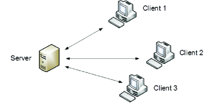
Figure 1: Client-server Interaction

The parameters $m,\,\epsilon,\,\gamma$ may be used to determine the time complexity and round complexity, where $\epsilon$ controls the accuracy of approximation, $\gamma$ controls the failure probability, and $m$ is the number of sets.

3 Preliminaries

During the accuracy analysis, Hoeffiding Inequality [24] and Chernoff Bound (see [32]) play an important role. They show how the number of samples determines the accuracy of approximation.

Theorem 5 ([24])

Let $X_{1},\,\ldots,\,X_{m}$ be $m$ independent random variables in $[0,\,1]$ and $X=\sum\limits_{i=1}^{m}X_{i}$.

i. If $X_{i}$ takes $1$ with probability at most $p$ for $i=1,\,\ldots,\,m$, then for any $\epsilon>0$, $\Pr(X>pm+\epsilon m)<e^{-{\epsilon^{2}m\over 2}}$.

ii. If $X_{i}$ takes $1$ with probability at least $p$ for $i=1,\,\ldots,\,m$, then for any $\epsilon>0$, $\Pr(X<pm-\epsilon m)<e^{-{\epsilon^{2}m\over 2}}$.

Theorem 6

Let $X_{1},\,\ldots,\,X_{m}$ be $m$ independent random $0$-$1$ variables, where $X_{i}$ takes $1$ with probability at least $p$ for $i=1,\,\ldots,\,m$. Let $X=\sum\limits_{i=1}^{m}X_{i}$, and $\mu=E[X]$. Then for any $\delta>0$, $\Pr(X<(1-\delta)pm)<e^{-{1\over 2}\delta^{2}pm}$.

Theorem 7

Let $X_{1},\,\ldots,\,X_{m}$ be $m$ independent random $0$-$1$ variables, where $X_{i}$ takes $1$ with probability at most $p$ for $i=1,\,\ldots,\,m$. Let $X=\sum\limits_{i=1}^{m}X_{i}$. Then for any $\delta>0$, $\Pr(X>(1+\delta)pm)<\left[{e^{\delta}\over(1+\delta)^{(1+\delta)}}\right]^{pm}$.

Define $g_{1}(\delta)=e^{-{1\over 2}\delta^{2}}$ and $g_{2}(\delta)={e^{\delta}\over(1+\delta)^{(1+\delta)}}$. Define $g(\delta)=\max\left(g_{1}(\delta),\,g_{2}(\delta)\right)$. We note that $g_{1}(\delta)$ and $g_{2}(\delta)$ are always strictly less than $1$ for all $\delta>0$. It is trivial for $g_{1}(\delta)$. For $g_{2}(\delta)$, this can be verified by checking that the function $f(x)=(1+x)\ln(1+x)-x$ is increasing and $f(0)=0$. This is because $f^{\prime}(x)=\ln(1+x)$ which is strictly greater than $0$ for all $x>0$.

We give a bound for ${e^{\delta}\over(1+\delta)^{(1+\delta)}}$. Let $u(x)={e^{x}\over(1+x)^{(1+x)}}$. We consider the case $x\in[0,\,1]$. We have

$$\ln u(x) = x-(1+x)\ln(1+x)\leq x-(1+x)(x-{x^{2}\over 2})=x-(x+{x^{2}\over 2}-{x^{3}\over 3})\leq-{x^{2}\over 6}.$$

Therefore,

$$u(x)\leq e^{-{x^{2}\over 6}}$$ (1)

for all $x\in[0,\,1]$. We let

$$g^{*}(x)=e^{-{x^{2}\over 6}}.$$ (2)

We have $g(x)\leq g^{*}(x)$ for all $x\in[0,\,1]$.

A well known fact, called union bound, in probability theory is the inequality

$$\Pr(E_{1}\cup E_{2}\ldots\cup E_{m})\leq\Pr(E_{1})+\Pr(E_{2})+\ldots+\Pr(E_{m}),$$

where $E_{1},\,E_{2},\,\ldots,\,E_{m}$ are $m$ events that may not be independent. In the analysis of our randomized algorithm, there are multiple events such that the failure from any of them may fail the entire algorithm. We often characterize the failure probability of each of those events, and use the above inequality to show that the whole algorithm has a small chance to fail after showing that each of them has a small chance to fail.

4 Algorithm Based on Adaptive Random Samplings

In this section, we develop a randomized algorithm for the size of set union when the approximate set sizes and biased random generators are given for the input sets. We give some definitions before the presentation of the algorithm. The algorithm developed in this section has an adaptive way to access the random generators from the input sets. All the random elements from input sets are generated in the beginning of the algorithm, and the number of random samples is known in the beginning of the algorithm. The results in this section show a tradeoff between the time complexity and the round complexity.

Definition 8

Let $L=A_{1},A_{2},\cdots,A_{m}$ be a list of finite sets.

1. For an element $x$, define $T(x,L)=\big{|}\{i:1\leq i\leq m$ and $x\in A_{i}\}\big{|}$.

2. For an element $x$, and a subset of indices with multiplicity $H$ of $\{1,2,\cdots,m\}$, define $S(x,H)=\big{|}\{i:i\in H$ and $x\in A_{i}\}\big{|}$.

3. Define ${\rm minThickness}(L)=\min\{T(x,L):x\in A_{1}\cup A_{2}\cup\cdots\cup A_{m}\}$.

4. Define ${\rm maxThickness}(L)=\max\{T(x,L):x\in A_{1}\cup A_{2}\cup\cdots\cup A_{m}\}$.

5. Let $W$ be a subset with multiplicity of $A_{1}\cup\cdots\cup A_{m}$, define $F(W,h,s)={s\over h}\sum\limits_{x\in W}{1\over T(x,L)}$, and $F^{\prime}(W)=\sum\limits_{x\in W}{1\over T(x,L)}={h\over s}F(W,h,s)$.

6. For a $\delta\in(0,1)$, partition $A_{1}\cup A_{2}\cup\cdots\cup A_{m}$ into $A_{1}^{\prime},\cdots,A_{k}^{\prime}$ such that $A_{i}^{\prime}=\{x:x\in A_{1}\cup A_{2}\cup\cdots\cup A_{m}$ and $T(x,L)\in[(1+\delta)^{i-1},(1+\delta)^{i})\}$ where $i=1,2,...,k.$ Define $v(\delta,z_{1},z_{2},L)=k$, which is the number of sets in the partition under the condition that $z_{1}\leq T(x,L)\leq z_{2}$.

4.1 Overview of Algorithm

We give an overview of the algorithm. For a list $L$ of input sets $A_{1},\cdots,A_{m}$, each set $A_{i}$ has an approximate size $m_{i}$ and a random generator. It is easy to see that $|A_{1}\cup A_{2}\cup\cdots\cup A_{m}|=\sum\limits_{i=1}^{m}\sum\limits_{x\in A_{i}}{1\over T(x,L)}$. The first phase of the algorithm generates a set $R_{1}$ of sufficient random samples from the list of input sets. The set $R_{1}$ has the property that ${m_{1}+\cdots+m_{m}\over|R_{1}|}\cdot\sum\limits_{x\in R_{1}}{1\over T(x,L)}$ is close to $\sum\limits_{i=1}^{m}\sum\limits_{x\in A_{i}}{1\over T(x,L)}$. We will use the variable $sum$ with initial value zero to approximate it. Each stage $i$ removes the set $V_{i}$ of elements from $R_{i}$ that each element $x\in V_{i}$ satisfies $T(x,L)\in\left[{T_{i}\over 4f_{1}(m)},T_{i}\right]$, and all elements $x\in R_{i}$ with $T(x,L)\in\left[{T_{i}\over f_{1}(m)},T_{i}\right]$ are in $V_{i}$, where $T_{i}=\max\{T(x,L):x\in R_{i}\}$ and $f_{1}(m)$ is a function at least $8$, which will determine the number of rounds, and the trade off between the running time and the number of rounds. In phase $i$, we choose a set $H_{i}$ of $u_{i}$ (to be large enough) of indices from $1,\cdots,m$, and use ${S(x,H_{i})m\over u_{i}}$ to approximate $T(x,L)$. It is accurate enough if $u_{i}$ is large enough. The elements left in $R_{i}-V_{i}$ will have smaller $T(x,L)$. The set $R_{i+1}$ will be built for the next stage $i+1$. When $R_{i}-V_{i}$ is shrinked to $R_{i+1}$ by random sampling in $R_{i}-V_{i}$, each element in $R_{i+1}$ will have its weight to be scaled by a factor ${|R_{i}-V_{i}|\over h_{i+1}}$. When an element $x$ is put into $V_{i}$, it is removed from $R_{i}$, and an approximate value of ${1\over T(x,L)}$ multiplied by its weight is added to $sum$. Finally, we will prove that $sum\cdot(m_{1}+\cdots+m_{m})$ is close to $\sum\limits_{i=1}^{m}\sum\limits_{x\in A_{i}}{1\over T(x,L)}$, which is equal to $|A_{1}\cup A_{2}\cup\cdots\cup A_{m}|$.

Example 1. Let $L$ be a list of $10$ sets $A_{1},\,A_{2},\,\cdots,\,A_{10},$ where $A_{i}=B_{i}\cup C$ with $|C|=1000$ and $|B_{i}|=100$ for $i=1,\,2,\,\cdots,\,10.$ In the beginning of the algorithm, we generate a set $R_{1}$ of $h_{1}=220$ random samples from list $L,$ where there are $200$ random samples with higher thickness $T(x,\,L),$ namely, these $200$ random samples locate in $C$ and $20$ random samples with lower thickness $T(x,\,L)$, say, these $20$ random samples locate in $B_{i}.$ At the first round, we only need select sets $A_{1},\,A_{3},$ and $A_{6}$ to approximate the thickness $T(x,\,L)$ of the $200$ random samples locating at $C.$ Then at the second round, we have to select all the sets $A_{1},\,A_{2},\,\cdots,\,A_{10},$ to approximate the thickness $T(x,\,L)$ of the $20$ random samples coming from $B_{i}$ (See Fig. 2).

Figure 2: Set Union of Ten Sets

4.2 Algorithm Description

Before giving the algorithm, we define an operation that selects a set of random elements from a list $L$ of sets $A_{1},\cdots,A_{m}$. We always assume $m\geq 2$ throughout the paper.

Definition 9

Let $L$ be a list of $m$ sets $A_{1},A_{2},\cdots,A_{m}$ with $m_{i}\in[(1-\beta_{L})|A_{i}|,(1+\beta_{R})|A_{i}|]$ and $(\alpha_{L},\alpha_{R})$-biased random generator RandomElement($A_{i}$) for $i=1,2,\cdots,m$, and $M=m_{1}+m_{2}+\cdots+m_{m}$. A random choice of $L$ is to get an element $x$ via the following two steps:

1. With probability ${m_{i}\over M}$, select a set $A_{i}$ among $A_{1},\cdots,A_{m}$.

2. Get an element $x$ from set $A_{i}$ via RandomElement$(A_{i})$.

We give some definitions about the parameters and functions that affect our algorithm below. We assume that $\epsilon\in(0,1)$ is used to control the accuracy of approximation, and $\gamma\in(0,1)$ is used to control the failure probability. Both parameters are from the input. In the following algorithm, the two integer parameters $z_{min}$ and $z_{max}$ with $1\leq z_{\min}\leq{\rm minThickness}(L)\leq{\rm maxThickness}(L)\leq z_{\max}\leq m$ can help speed up the computation. The algorithm is still correct if we use default case with $z_{min}=1$ and $z_{max}=m$.

1. The following parameters are used to control the accuracy of approximation at different stages of algorithm:

   $$\epsilon_{0} = {\epsilon\over 9},\epsilon_{1}={\epsilon_{0}\over 6(\log{m})},\epsilon_{2}={\epsilon_{1}\over 4},\epsilon_{3}={\epsilon_{0}\over 3},$$ (3)

   $$\delta = {\epsilon_{2}\over 2}.$$ (4)

2. The following parameters are used to control the failure probability at several stages of the algorithm:

   $$\gamma_{1} = {\gamma\over 3},\gamma_{2}={\gamma\over 6\log{m}}.$$ (5)

3. Function $f_{1}(.)$ is used to control the number of rounds of the algorithm. Its growth rate is mainly determined by the parameter $c_{1}$ that will be determined later:

   $$f_{1}(m) = 8m^{c_{1}}\ {\rm with\ }c_{1}\geq 0,$$ (6)

4. Function $f_{2}(.)$ is used to check the number of random samples in $A_{j}^{\prime}$ of Stage $1$ in the algorithm. We will use different ways to control the accuracy of approximation between the case $|A_{i}|\leq{|A_{1}\cup A_{2}\cup\cdots\cup A_{m}|\over f_{2}(m)}$ and the other case $|A_{i}|>{|A_{1}\cup A_{2}\cup\cdots\cup A_{m}|\over f_{2}(m)}$. It is mainly used in the proof of Lemma 15 that shows it keeps the accuracy of approximation when algorithm goes from Stage $i$ to Stage $i+1$.

   $$f_{2}(m) = {2v(\delta,z_{\min},z_{\max},L)\over\epsilon_{3}}+{2\log{{m}\over z_{\min}}\over\epsilon_{3}\log(1+\delta)}.$$ (7)

5. Function $f_{3}(.)$ is used as a threshold to count the number $t_{i,j}$ of random samples in $R_{i}\cap A_{j}^{\prime}$ of Stage $i$ in the algorithm. We will use different ways to control the accuracy of approximation between the case $t_{i,j}\leq f_{3}(m)$ and the other case $t_{i,j}>f_{3}(m)$. It is mainly used in the proof of Lemma 12 that shows that the number of random samples at Stage $1$ will provide enough accuracy of approximation.

   $$f_{3}(m) = {f_{1}(m)}\cdot{6\ln{2\over\gamma_{2}}\over\epsilon_{2}^{2}}.$$ (8)

6. Function $f_{4}(.)$ is used to determine the growth rate of function Function $f_{5}(.)$, which is defined by equation (10).

   $$f_{4}(m) = {f_{2}(m)\log{{m}^{2}\over\epsilon_{1}}\over 6\epsilon_{1}^{2}}+{f_{3}(m)\over\epsilon_{2}f_{1}(m)}.$$ (9)

7. Function $f_{5}(.)$ determines the number of random samples from the input sets in the beginning of the algorithm:

   $$f_{5}(m) = {mf_{4}(m)\over z_{\min}}.$$ (10)

8. The following parameter is also used to control failure probability in a stage of the algorithm:

   $$\gamma_{3} = {\gamma_{2}\over 2f_{5}(m)}.$$ (11)

9. Function $f_{6}(.)$ affects the number of random indices in the range $\{1,2,\cdots,m\}$. Those random indices will be used to choose input sets to detect the approximate $T(x,L)$ for those random samples $x$:

   $$f_{6}(m) = f_{1}(m)\left({24\over\epsilon_{1}^{2}}\cdot{\ln{2\over\gamma_{3}}}\right).$$ (12)

Algorithm 1 ApproximateUnion($L,z_{\min},z_{\max},M,\gamma,\epsilon$)

$\mathbf{Input:}$ $L$ is a list of $m$ sets $A_{1},A_{2},\cdots,A_{m}$ with $m\geq 2$, $m_{i}\in[(1-\beta_{L})|A_{i}|,(1+\beta_{R})|A_{i}|]$ and $(\alpha_{L},\alpha_{R})$-biased random generator RandomElement($A_{i}$) for $i=1,2,\cdots,m$, integers $z_{min}$ and $z_{max}$ with $1\leq z_{\min}\leq minThickness(L)\leq maxThickness(L)\leq z_{\max}\leq m$, parameter $\gamma\in(0,1)$ to control the failure probability, parameter $\epsilon\in(0,1)$ to control the accuracy of approximation, and $M=m_{1}+m_{2}+\cdots+m_{m}$ as the sum of sizes of input sets.
$\mathbf{Output:}$ $sum\cdot M.$

1:  Let $h_{1}=f_{5}(m)$

2:  Let $i=1$

3:  Let currentThickness${}_{1}=z_{max}$

4:  Let $s_{1}={m\over{currentThickness_{1}}}$

5:  Let $s_{1}^{\prime}=1$

6:  Let $sum=0$

7:  Obtain a set $R_{1}$ of $h_{1}$ random choices of $L$ (see Definition 9)

8:  Stage $i$

9:    Let $u_{i}=s_{i}\cdot f_{6}(m)$

10:    Select $u_{i}$ random indices $H_{i}=\{k_{1},\cdots,k_{u_{i}}\}$ from $\{1,2,\cdots,m\}$

11:    Compute $S(x,H_{i})$ for each $x\in R_{i}$

12:    Let $V_{i}$ be the subset of $R_{i}$ with elements $x$ satisfying $S(x,H_{i})\geq\frac{currentThickness_{i}}{2f_{1}(m)\cdot m}\cdot u_{i}$

13:    Let $sum=sum+s_{i}^{\prime}\sum\limits\limits_{x\in V_{i}}{u_{i}\over S(x,H_{i})m}$

14:    Let $currentThickness_{i+1}={currentThickness_{i}\over f_{1}(m)}$

15:    Let $s_{i+1}={m\over currentThickness_{i+1}}$

16:    Let $h_{i+1}={h_{1}\over s_{i+1}}$

17:    If $(|R_{i}|-|V_{i}|<h_{i+1})$

18:    Then

19:    $\{$

20:      Let $R_{i+1}=R_{i}-V_{i}$

21:      Let $a_{i}=1$

22:    }

23:    Else

24:    {

25:      Let $R_{i+1}$ be a set of random $h_{i+1}$ samples from $R_{i}-V_{i}$

26:      Let $a_{i}={|R_{i}|-|V_{i}|\over h_{i+1}}$

27:    }

28:    Let $s_{i+1}^{\prime}=s_{i}^{\prime}\cdot a_{i}$

29:    Let $i=i+1$

30:    If ($currentThickness_{i}<z_{min}$)

31:      Return $sum\cdot M$ and terminate the algorithm

32:    Else

33:      Enter the next Stage $i$

We let $M=m_{1}+m_{2}+\cdots+m_{m}$ and $z_{\min}$ be part of the input of the algorithm. It makes the algorithm be possible to run in a sublinear time when $z_{\min}\geq m^{a}$ for a fixed $a>0$. Otherwise, the algorithm has to spend $\Omega(m)$ time to compute $M$.

4.3 Proof of Algorithm Performance

The accuracy and complexity of algorithm ApproximateUnion(.) will be proven in the following lemmas. Lemma 10 gives some basic properties of the algorithm. Lemma 12 shows that $R_{1}$ has random samples are used so that $F(R_{1},h_{1},1)\left(\sum\limits_{i=1}^{m}m_{i}\right)$ is an accurate approximation for $\sum\limits_{i=1}^{m}\sum\limits_{x\in A_{i}}{1\over T(x,L)}$.

Lemma 10

The algorithm ApproximateUnion(.) has the following properties:

1. $g^{*}(\epsilon_{1})^{f_{4}(m)\over f_{2}(m)}\leq{\epsilon_{1}\over m^{2}}$.

2. $v(\delta,z_{\min},z_{\max},L)={\rm O}\left({\log{z_{\max}\over z_{\min}}\over\delta}\right)$.

3. ${2v(\delta,z_{\min},z_{\max},L)\over f_{2}(m)}\leq\epsilon_{3}$ and $f_{2}(m)={\rm O}\left({\log{m\over z_{\min}}\over\delta\epsilon_{3}}\right)$.

4. $R_{i}$ contains at most $h_{i}$ items.

5. $g^{*}(\epsilon_{2})^{f_{3}(m)\over f_{1}(m)}\leq{\gamma_{2}\over 2}$.

6. $f_{4}(m)={\rm O}\left({1\over\epsilon^{4}}\left(\log{m\over z_{\min}}\right)\cdot\log{{m}\over\epsilon}\cdot\left(\log{m}\right)^{3}+{(\log m)^{3}(\ln{1\over\gamma}+\log m)\over\epsilon^{3}}\right)$.

7. $f_{6}(m)={\rm O}\left({m^{c_{1}}\over\epsilon^{2}}\cdot(\log m)^{2}(\log{2\over\gamma}+\log m+\log f_{4}(m))\right)$.

Proof:  The statements are easily proven according to the setting in the algorithm.

Statement  i: It follows from equations (2) and (9).

Statement  ii: By Definition 8, we need $v(\delta,z_{\min},z_{\max},L)$ with $z_{min}(1+\delta)^{v(\delta,z_{\min},z_{\max},L)}\geq z_{max}$. Thus, we have $v(\delta,z_{\min},z_{\max},L)\leq 2\left({\log{z_{\max}\over z_{\min}}\over\log(1+\delta)}\right)={\rm O}\left({\log{z_{\max}\over z_{\min}}\over\delta}\right)$ since $\log(1+\delta)=\Theta(\delta)$.

Statement  iii: It is easy to see that $\log(1+\delta)=\Theta(\delta)$ and $1\leq z_{max}\leq m$. It follows from equation (7), and Statement  ii.

Statement  iv: It follows from lines 19 to 27 in the algorithm.

Statement v: It follows from equation (8).

Statement  vi: By equation (9), Statement iii and equation (3), we have

$$f_{4}(m) = {f_{2}(m)\log{{m}^{2}\over\epsilon_{1}}\over 6\epsilon_{1}^{2}}+{f_{3}(m)\over\epsilon_{2}f_{1}(m)}$$

$$\leq \left(6f_{2}(m)\cdot\log{{m}^{2}\over\epsilon_{1}}\cdot\left({\log{m}\over\epsilon_{0}}\right)^{2}+{f_{3}(m)\over\epsilon_{2}f_{1}(m)}\right)$$

$$= {\rm O}\left(f_{2}(m)\cdot\log{{m}^{2}\over\epsilon_{1}^{2}}\cdot\left({\log{m}\over\epsilon_{0}}\right)^{2}+{1\over\epsilon_{2}}\cdot{\ln{2\over\gamma_{2}}\over\epsilon_{2}^{2}}\right)$$

$$= {\rm O}\left({1\over\delta\epsilon_{3}\epsilon_{0}^{2}}(\log{m\over z_{\min}})\cdot\log{{m}\over\epsilon_{1}}\cdot(\log{m})^{2}+{\log m\over\epsilon_{0}}\cdot{\ln{2\over\gamma_{2}}\over\epsilon_{2}^{2}}\right)$$

$$= {\rm O}\left({1\over\delta\epsilon_{3}\epsilon_{0}^{2}}(\log{m\over z_{\min}})\cdot\log{{m}\over\epsilon_{1}}\cdot(\log{m})^{2}+{\log m\over\epsilon_{0}}\cdot{\ln{2\over\gamma_{2}}\over\epsilon_{2}^{2}}\right)$$

$$= {\rm O}\left({1\over\epsilon^{4}}\left(\log{m\over z_{\min}}\right)\cdot\log{{m}\over\epsilon}\cdot\left(\log{m}\right)^{3}+{(\log m)^{3}(\ln{1\over\gamma}+\log m)\over\epsilon^{3}}\right).$$

Statement vii: By equation (12), we have

$$f_{6}(m) = f_{1}(m)\left({24\over\epsilon_{1}^{2}}\cdot{\ln{2\over\gamma_{3}}}\right)$$ (13)

$$= {\rm O}\left({m^{c_{1}}\over\epsilon_{1}^{2}}\cdot{\ln{2\over\gamma_{3}}}\right)$$ (14)

$$= {\rm O}\left({m^{c_{1}}\over\epsilon^{2}}\cdot(\log m)^{2}(\log{2\over\gamma_{2}}+\ln f_{5}(m))\right)$$ (15)

$$= {\rm O}\left({m^{c_{1}}\over\epsilon^{2}}\cdot(\log m)^{2}(\log{2\over\gamma_{2}}+\ln m+\ln f_{4}(m))\right)$$ (16)

$$= {\rm O}\left({m^{c_{1}}\over\epsilon^{2}}\cdot(\log m)^{2}(\log{2\over\gamma_{2}}+\log m+\log f_{4}(m))\right)$$ (17)

$$= {\rm O}\left({m^{c_{1}}\over\epsilon^{2}}\cdot(\log m)^{2}(\log{2\over\gamma}+\log m+\log f_{4}(m))\right).$$ (18)

 

Lemma 11 gives an upper bound for the number of rounds for the algorithm. It shows how round complexity depends on $z_{max},z_{min}$ and $f_{1}(.)$.

Lemma 11

The number of rounds of the algorithm is ${\rm O}\left({\log{z_{max}\over z_{min}}\over\log f_{1}(m)}\right)$.

Proof:  By line 3 of the algorithm, we have ${\rm currentThickness}_{1}=z_{max}$. Variable
${\rm currentThickness}_{i}$ is reduced by a factor $f_{1}(m)$ each phase as ${\rm currentThickness}_{i+1}={{\rm currentThickness}_{i}\over f_{1}(m)}$ by line 14 of the algorithm. By the termination condition of line 30 of the algorithm, if $y$ is the number of phases of the algorithm, we have $y\leq y^{\prime}$, where $y^{\prime}$ is any integer with ${z_{max}\over f_{1}(m)^{y^{\prime}}}<z_{min}$. Thus, $y={\rm O}\left({\log{z_{max}\over z_{min}}\over\log f_{1}(m)}\right)$.         

Lemma 12 shows the random samples, which are saved in $R_{1}$ in the beginning of the algorithm, will be enough to approximate the size of set union via $F(R_{1},h_{1},1)M$. In the next a few rounds, algorithm will approximate $F(R_{1},h_{1},1)$.

Lemma 12

With probability at least $1-\gamma_{1}$, $F(R_{1},h_{1},1)M\in[\frac{(1-\epsilon_{0}){(1-\alpha_{L})(1-\beta_{L})}}{1+\delta}|A_{1}\cup\cdots\cup A_{m}|,\,(1+\epsilon_{0}){(1+\alpha_{R})(1+\beta_{R})(1+\delta)}|A_{1}\cup\cdots\cup A_{m}|]$.

Proof:  Let $A=|A_{1}\cup\cdots\cup A_{m}|$ and $U=|A_{1}|+|A_{2}|+\cdots+|A_{m}|$. For an arbitrary set $A_{i}$ in the list $L$, and an arbitrary element $x\in A_{i}$, with at least the following probability $x$ is selected via ${\rm RandomElement}(A_{i})$ at line 7 of Algorithm ApproximateUnion(.),

$${m_{i}\over m_{1}+m_{2}+\cdots+m_{m}}{1-\alpha_{L}\over|A_{i}|} \geq {(1-\beta_{L})|A_{i}|\over M}{1-\alpha_{L}\over|A_{i}|}$$

$$= {(1-\beta_{L})(1-\alpha_{L})\over M}.$$

Similarly, with at most the following probability $x$ is chosen via ${\rm RandomElement}(A_{i})$ at line 7 of Algorithm ApproximateUnion(.),

$${m_{i}\over m_{1}+m_{2}+\cdots+m_{m}}{1+\alpha_{R}\over|A_{i}|} \leq {(1+\beta_{R})|A_{i}|\over M}{1+\alpha_{R}\over|A_{i}|}$$

$$= {(1+\beta_{R})(1+\alpha_{R})\over M}.$$

Define $\rho_{L}=1-{(1-\beta_{L})(1-\alpha_{L})}$ and $\rho_{R}={(1+\beta_{R})(1+\alpha_{R})}-1$. Each element $x$ in $A_{1}\cup A_{2}\cup\cdots\cup A_{m}$ is selected with probability in $\left[{(1-\rho_{L})T(x,L)\over M},{(1+\rho_{R})T(x,L)\over M}\right]$.

Define $T_{1}=\left\{A_{j}^{\prime}:|A_{j}^{\prime}|\leq{A\over f_{2}(m)}\right\}$, and $T_{2}=\left\{A_{j}^{\prime}:|A_{j}^{\prime}|>{A\over f_{2}(m)}\right\}$ (see  vi of Definition 8). Let $t_{j}=\min\left\{T(x,L):x\in A_{j}^{\prime}\right\}$. We discuss two cases:

Case 1: $A_{j}^{\prime}\in T_{1}$. When one element $x$ is chosen, the probability that $x\in A_{j}^{\prime}$ is in the range $\left[{(1-\rho_{L})t_{j}|A_{j}^{\prime}|\over M},{(1+\rho_{R})(1+\delta)t_{j}|A_{j}^{\prime}|\over M}\right]$. Let $p_{j}={(1+\rho_{R})(1+\delta)t_{j}\cdot{A\over f_{2}(m)}\over M}$. Since $z_{\min}\leq{\rm minThickness}(L)$, we have $z_{\min}\leq{\rm minThickness}(L)\leq t_{j}$. It is easy to see that $mA\geq U$. We have

$$p_{j}h_{1} = {(1+\rho_{R})(1+\delta)t_{j}\cdot{A\over f_{2}(m)}\over M}\cdot{mf_{4}(m)\over z_{\min}}$$ (19)

$$\geq {(1+\rho_{R})(1+\delta)\cdot f_{4}(m)mA\over f_{2}(m)M}$$

$$\geq {(1+\rho_{R})(1+\delta)\cdot f_{4}(m)U\over f_{2}(m)M}$$

$$\geq {(1+\rho_{R})(1+\delta)\cdot f_{4}(m)\over f_{2}(m)(1+\beta_{R})}$$

$$= {(1+\alpha_{R})(1+\delta)\cdot f_{4}(m)\over f_{2}(m)}.$$

Let $\omega_{1}(m)={(1+\alpha_{R})(1+\delta)\cdot f_{4}(m)\over f_{2}(m)}$. Thus, $p_{j}h_{1}\geq\omega_{1}(m)$.

Let $R_{1,j}$ be the elements of $R_{1}$ and also in $A_{j}^{\prime}$. By Theorem 7, with probability at most $P_{j}=g^{*}(1)^{p_{j}\cdot h_{1}}\leq g^{*}(1)^{\omega_{1}(m)}\leq{\gamma_{1}\over 2}$ (by equation (7), equation (9) and inequality (19)), there are more than $2p_{j}h_{1}={2(1+\rho_{R})(1+\delta)t_{j}\cdot{A\over f_{2}(m)}\over M}\cdot h_{1}$ elements to be chosen from $A_{j}^{\prime}$ into $R_{1}$. Thus,

$$F^{\prime}(R_{1,j})\leq{2p_{j}h_{1}\over t_{j}}={2(1+\rho_{R})(1+\delta)\cdot A\over f_{2}(m)M}\cdot h_{1},$$ (20)

with probability at most $P_{j}$ to fail.

Case 2: $A_{j}^{\prime}\in T_{2}$. When $h_{1}$ elements are selected to $R_{1}$, let $v_{j}$ be the number of elements selected in $A_{j}^{\prime}$. When one element $x$ is chosen, the probability that $x\in A_{j}^{\prime}$ is in the range $\left[{(1-\rho_{L})t_{j}|A_{j}^{\prime}|\over M},{(1+\rho_{R})(1+\delta)t_{j}|A_{j}^{\prime}|\over M}\right]$.

Let $p_{j,1}={(1-\rho_{L})t_{j}|A_{j}^{\prime}|\over M}$ and $p_{j,2}={(1+\rho_{R})(1+\delta)t_{j}|A_{j}^{\prime}|\over M}$.

We have

$$p_{j,1}h_{1} = {(1-\rho_{L})t_{j}|A_{j}^{\prime}|\over M}\cdot h_{1}$$ (21)

$$> {(1-\rho_{L})t_{j}{A\over f_{2}(m)}\over M}\cdot h_{1}\geq{(1-\rho_{L})z_{min}A\cdot h_{1}\over f_{2}(m)M}={(1-\rho_{L})z_{min}A\cdot mf_{4}(m)\over z_{min}f_{2}(m)M}$$

$$\geq {(1-\rho_{L})f_{4}(m)\over f_{2}(m)(1+\beta_{R})}.$$

We have

$$p_{j,2}h_{1} = {(1+\rho_{R})(1+\delta)t_{j}|A_{j}^{\prime}|\over M}\cdot h_{1}$$ (22)

$$> {(1+\rho_{R})(1+\delta)t_{j}\cdot{A\over f_{2}(m)}\over M}\cdot h_{1}$$

$$\geq {(1+\rho_{R})(1+\delta)z_{min}\cdot A\over f_{2}(m)M}\cdot h_{1}$$

$$= {(1+\rho_{R})(1+\delta)z_{min}\cdot A\over f_{2}(m)M}\cdot{mf_{4}(m)\over z_{min}}$$

$$\geq {(1+\rho_{R})(1+\delta)\cdot f_{4}(m)\over f_{2}(m)(1+\beta_{R})}$$

$$\geq {(1+\alpha_{R})(1+\delta)\cdot f_{4}(m)\over f_{2}(m)}.$$

With probability at most $g^{*}(\epsilon_{3})^{p_{j,1}\cdot h_{1}}\leq{\gamma_{1}\over 4}$ (by equation (7), equation (9) and inequality (21)),

$$v_{j}<{(1-\epsilon_{3})(1-\rho_{L})t_{j}|A_{j}^{\prime}|\over M}\cdot h_{1}=(1-\epsilon_{3})(1-\rho_{L})t_{j}h_{1}\cdot{|A_{j}^{\prime}|\over M}.$$

With probability at most $g^{*}(\epsilon_{3})^{p_{j,2}\cdot h_{1}}\leq{\gamma_{1}\over 4}$ (by equation (7), equation (9) and inequality (22)),

$$v_{j}>{(1+\epsilon_{3})(1+\rho_{R})(1+\delta)t_{j}|A_{j}^{\prime}|\over M}\cdot h_{1}=(1+\epsilon_{3})(1+\rho_{R})(1+\delta)t_{j}h_{1}\cdot{|A_{j}^{\prime}|\over M}.$$

Therefore, with probability at least $1-\gamma_{1}/2$, we have

$$v_{j}\in\left[(1-\epsilon_{3})(1-\rho_{L})t_{j}h_{1}\cdot{|A_{j}^{\prime}|\over M},(1+\epsilon_{3})(1+\rho_{R})(1+\delta)t_{j}h_{1}\cdot{|A_{j}^{\prime}|\over M}\right].$$ (23)

Thus, we have that there are sufficient elements of $A_{j}^{\prime}$ to be selected with high probability, which follows from Theorem 6 and Theorem 7.

In the rest of the proof, we assume that inequality (20) holds if the condition of Case 1 holds, and inequality (23) holds if the condition of Case 2 holds.

Now we consider

$$F(R_{1},h_{1},1)={1\over h_{1}}\sum\limits_{x\in R_{1}}{1\over T(x,L)}$$ (24)

$$= {1\over h_{1}}\left(\sum\limits_{R_{1,j}\ with\ A_{j}^{\prime}\in T_{1}}\sum\limits_{x\in R_{1,j}}{1\over T(x,L)}+\sum\limits_{R_{1,j}\ with\ A_{j}^{\prime}\in T_{2}}\sum\limits_{x\in R_{1,j}}{1\over T(x,L)}\right)$$

$$\leq {1\over h_{1}}{2(1+\rho_{R})(1+\delta)v(\delta,z_{\min},z_{\max},L)\cdot A\over f_{2}(m)M}\cdot h_{1}$$

$$+\frac{1}{h_{1}}\sum\limits_{R_{1,j}\ with\ A_{j}^{\prime}\in T_{2}}\sum\limits_{x\in R_{1,j}}{1\over T(x,L)}$$

$$\leq {1\over h_{1}}\left({2(1+\rho_{R})(1+\delta)v(\delta,z_{\min},z_{\max},L)\cdot A\over f_{2}(m)M}\cdot h_{1}+\sum\limits_{R_{1,j}\ with\ A_{j}^{\prime}\in T_{2}}{v_{j}\over t_{j}}\right)$$

$$\leq {1\over h_{1}}\left({2(1+\rho_{R})(1+\delta)v(\delta,z_{\min},z_{\max},L)\cdot A\over f_{2}(m)M}\cdot h_{1}\right)$$

$$+{1\over h_{1}}\left(\sum\limits_{R_{1,j}\ with\ A_{j}^{\prime}\in T_{2}}{(1+\epsilon_{3})(1+\rho_{R})(1+\delta)h_{1}\cdot{|A_{j}^{\prime}|\over M}}\right)$$

$$= {2(1+\rho_{R})(1+\delta)v(\delta,z_{\min},z_{\max},L)\cdot A\over f_{2}(m)M}$$

$$+\sum\limits_{R_{1,j}\ with\ A_{j}^{\prime}\in T_{2}}{(1+\epsilon_{3})(1+\rho_{R})(1+\delta)\cdot{|A_{j}^{\prime}|\over M}}$$

$$\leq \left({2(1+\rho_{R})(1+\delta)v(\delta,z_{\min},z_{\max},L)\over f_{2}(m)}+(1+\epsilon_{3})(1+\rho_{R})(1+\delta)\right){A\over M}$$

$$= \left(1+\epsilon_{3}+{2v(\delta,z_{\min},z_{\max},L)\over f_{2}(m)}\right)(1+\rho_{R})(1+\delta){A\over M}$$

$$\leq (1+2\epsilon_{3})(1+\rho_{R})(1+\delta){A\over M}$$

$$\leq (1+\epsilon_{0})(1+\rho_{R})(1+\delta){A\over M}.$$

The transition from (24) to (4.3) is by Statement iii of Lemma 10. For the lower bound part, we have the following inequalities:

$$F(R_{1},h_{1},1)={1\over h_{1}}\sum\limits_{x\in R_{1}}{1\over T(x,L)}$$ (26)

$$\geq {1\over h_{1}}\left(\sum\limits_{R_{1,j}\ with\ A_{j}^{\prime}\in T_{2}}\sum\limits_{x\in R_{1,j}}{1\over T(x,L)}\right)$$

$$\geq {1\over h_{1}}\left(\sum\limits_{R_{1,j}\ with\ A_{j}^{\prime}\in T_{2}}{v_{j}\over(1+\delta)t_{j}}\right)$$

$$\geq {1\over h_{1}}\left(\sum\limits_{R_{1,j}\ with\ A_{j}^{\prime}\in T_{2}}{(1-\epsilon_{3})(1-\rho_{L})h_{1}\cdot{|A_{j}^{\prime}|\over(1+\delta)M}}\right)$$

$$= {(1-\epsilon_{3})(1-\rho_{L})\over(1+\delta)M}\left(\sum\limits_{R_{1,j}\ with\ A_{j}^{\prime}\in T_{2}}|A_{j}^{\prime}|\right)$$

$$= {(1-\epsilon_{3})(1-\rho_{L})\over(1+\delta)M}\sum\limits_{R_{1,j}\ with\ A_{j}^{\prime}\in T_{1}}|A_{j}^{\prime}|+{(1-\epsilon_{3})(1-\rho_{L})\over(1+\delta)M}\sum\limits_{R_{1,j}\ with\ A_{j}^{\prime}\in T_{2}}|A_{j}^{\prime}|$$

$$-{(1-\epsilon_{3})(1-\rho_{L})\over(1+\delta)M}\sum\limits_{R_{1,j}\ with\ A_{j}^{\prime}\in T_{1}}|A_{j}^{\prime}|$$

$$= {(1-\epsilon_{3})(1-\rho_{L})\over(1+\delta)M}\left(A-\sum\limits_{R_{1,j}\ with\ A_{j}^{\prime}\in T_{1}}|A_{j}^{\prime}|\right)$$

$$\geq {(1-\epsilon_{3})(1-\rho_{L})\over(1+\delta)M}\left(A-{v(\delta,z_{\min},z_{\max},L)A\over f_{2}(m)}\right)$$

$$= \left(1-{v(\delta,z_{\min},z_{\max},L)\over f_{2}(m)}\right)\frac{(1-\epsilon_{3})(1-\rho_{L})}{(1+\delta)}{A\over M}$$

$$\geq (1-\epsilon_{3})\frac{(1-\epsilon_{3})(1-\rho_{L})}{(1+\delta)}{A\over M}$$

$$\geq \frac{(1-\epsilon_{0})(1-\rho_{L})}{(1+\delta)}{A\over M}.$$

The transition from (26) to (4.3) is by Statement $3$ of Lemma 10. Therefore, $F(R_{1},h_{1},1)M\in\left[\frac{(1-\epsilon_{0})(1-\rho_{L})}{(1+\delta)}A,\,(1+\epsilon_{0})(1+\rho_{R})(1+\delta)A\right]$.         

Lemma 13 shows that at stage $i$, it can approximate $T(x,L)$ for all random samples with highest $T(x,L)$ in $R_{i}$. Those random elements with highest $T(x,L)$ will be removed in stage $i$ so that the algorithm will look for random elements with smaller $T(x,L)$ in the coming stages.

Lemma 13

After the execution of Stage $i$, with probability at least $1-\gamma_{2}$, we have the following three statements:

1. Every element $x\in R_{i}$ with $T(x,L)\geq{{\rm currentThickness}_{i}\over 4f_{1}(m)}$ has $S(x,H_{i})\in$
   $\left[(1-\epsilon_{1}){T(x,L)\over{m}}u_{i},(1+\epsilon_{1}){T(x,L)\over{m}}u_{i}\right]$.

2. Every element $x\in V_{i}$ with $T(x,L)\geq{{\rm currentThickness}_{i}\over f_{1}(m)}$, it satisfies the condition in line 12 of the algorithm.

3. Every element $x\in V_{i}$ with $T(x,L)<{{\rm currentThickness}_{i}\over 4f_{1}(m)}$, it does not satisfy the condition in line 12 of the algorithm.

Proof:  It follows from Theorem 6 and Theorem 7. There are $u_{i}=s_{i}f_{6}(m)$ indices are selected among $\{1,2,\cdots,m\}$. Let $p={T(x,L)\over{m}}$.

Statment i: We have $pu_{i}={T(x,L)\over{m}}\cdot s_{i}f_{6}(m)\geq{{\rm currentThickness}_{i}\over 4f_{1}(m)}\cdot{1\over{m}}\cdot s_{i}f_{6}(m)={{\rm currentThickness}_{i}\over 4f_{1}(m)}\cdot{1\over{m}}\cdot{m\over{\rm currentThickness}_{i}}\cdot f_{6}(m)={f_{6}(m)\over 4f_{1}(m)}$.

With probability at most $P_{1}=g^{*}(\epsilon_{1})^{pu_{i}}\leq{\gamma_{3}\over 2}$ (by equations (8), and (12)), $S(x,H_{i})<(1-\epsilon_{1}){T(x,L)\over{m}}u_{i}$. With probability at most $P_{2}=g^{*}(\epsilon_{1})^{pu_{i}}\leq{\gamma_{3}\over 2}$ (by equations (8) and (12)), $S(x,H_{i})>(1+\epsilon_{1}){T(x,L)\over{m}}u_{i}$.

There are at most $h_{i}$ elements in $R_{i}$ by Statement iv of Lemma 10. Therefore, with probability at most $h_{i}(P_{1}+P_{2})\leq h_{1}(P_{1}+P_{2})\leq h_{1}\cdot\gamma_{3}={\gamma_{2}\over 2}$,

$$S(x,H_{i})\not\in\left[(1-\epsilon_{1}){T(x,L)\over{m}}u_{i},(1+\epsilon_{1}){T(x,L)\over{m}}u_{i}\right].$$

Statement ii: This statement of the lemma follows from Statement i.

Statement iii: This part of the lemma follows from Theorem 6 and Theorem 7. For $x\in V_{i}$ with $T(x,L)<{{\rm currentThickness}_{i}\over 4f_{1}(m)}$, let $p={{\rm currentThickness}_{i}\over 4f_{1}(m)}$. With probability at most $g^{*}(1)^{pu_{i}}\leq{\gamma_{3}\over 2}$ (by equations (8), and (12)), we have $S(x,H_{i})\geq 2pu_{i}$. There are at most $h_{i}$ elements in $R_{i}$ by Statement iv of Lemma 10. Therefore, with probability at most $h_{1}\cdot\gamma_{3}\leq{\gamma_{2}\over 2}$, there exists one $x\in V_{i}$ with $T(x,L)<{{\rm currentThickness}_{i}\over 4f_{1}(m)}$ to satisfy $S(x,H_{i})\geq 2pu_{i}$.         

Lemma 14

Let $x$ and $y$ be positive real numbers with $1\leq y$. Then we have:

1. $1-xy<(1-x)^{y}$.

2. If $xy<1$, then $(1+x)^{y}<1+2xy$.

3. If $x_{1},x_{2}\in[0,1)$, then $1-x_{1}-x_{2}\leq(1-x_{1})(1-x_{2})$, and $(1+x_{1})(1+x_{2})\leq 1+2x_{1}+x_{2}$.

Proof:  By Taylor formula, we have $(1-x)^{y}=1-xy+{y\cdot(y-1)\over 2}\theta^{2}$ for some $\theta\in[0,x]$. Thus, we have $(1-x)^{y}\geq 1-yx$. Note that the function $(1+{1\over z})^{z}$ is increasing, and $\lim_{z\rightarrow+\infty}(1+{1\over z})^{z}=e$. We also have $(1+x)^{y}\leq(1+x)^{{1\over x}\cdot xy}\leq e^{xy}\leq 1+xy+(xy)^{2}\leq 1+2xy$.

It is trivial to verify Statement iii. $1-x_{1}-x_{2}\leq(1-x_{1})(1-x_{2})$. Clearly, $(1+x_{1})(1+x_{2})=1+x_{1}+x_{2}+x_{1}x_{2}\leq 1+2x_{1}+x_{2}$.         

Lemma 15 shows that how to gradually approximate $F(R_{1},h_{1},1)M$ via several rounds. It shows that the left random samples stored in $R_{i+1}$ after stage $i$ is enough to approximate $F^{\prime}(R_{i}-V_{i})$.

Lemma 15

Let $y$ be the number of stages. Let $V_{i}$ be the set of elements removed from $R_{i}$ in Stage $i$. Then we have the following facts:

1. With probability at least $1-\gamma_{2}$, $a_{i}F^{\prime}(R_{i+1})\in[(1-\epsilon_{1})F^{\prime}(R_{i}-V_{i}),(1+\epsilon_{1})F^{\prime}(R_{i}-V_{i})]$, and

2. With probability at least $1-2y\gamma_{2}$, $\sum_{i=1}^{y}s_{i}^{\prime}F^{\prime}(V_{i})\in[(1-y\epsilon_{1})S,(1+2y\epsilon_{1})S]$, where $S=F(R_{1},h_{1},1)$.

Proof: Let $h_{i}^{\prime}=h_{i}-|V_{i}|$. If an local is too small, it does not affect the global sum much. In $R_{i+1}$, we deal with the elements $x$ of $T(x,L)<{{\rm currentThickness}_{i}\over f_{1}(m)}$. By Lemma 13, with probability at least $1-\gamma_{2}$, $R_{i}-V_{i}$ does not contain any $x$ with $T(x,L)\geq{{\rm currentThickness}_{i}\over f_{1}(m)}$.

Let $t_{i,j}$ be the number of elements of $A_{j}^{\prime}$ in $R_{i}$ with multiplicity. Let $B_{i,j}$ be the set of elements in both $R_{i}$ and $A_{j}^{\prime}$ with multiplicity.

Statement i: We discuss two cases:

Case 1: $|R_{i}|-|V_{i}|<h_{i+1}$. This case is trivial since $R_{i+1}=R_{i}-V_{i}$ and $a_{i}=1$ according to the algorithm (line (19) to line (22)).

In the following Case 2, we assume the condition of Case 1 is false. Thus, $h_{i}^{\prime}\geq h_{i+1}$.

Case 2: $|R_{i}|-|V_{i}|\geq h_{i+1}$. We have

$$F^{\prime}(R_{i}-V_{i}) \geq {h_{i}^{\prime}\over{{\rm currentThickness}_{i}\over f_{1}(m)}}\geq{h_{i+1}\over{{\rm currentThickness}_{i}\over f_{1}(m)}}$$ (28)

$$= {{h_{1}\over s_{i+1}}\cdot f_{1}(m)\over{\rm currentThickness}_{i}}={f_{4}(m)\over z_{min}}.$$

Two subcases are discussed below.

Subcase 2.1: $t_{i,j}\leq f_{3}(m)$, in this case, $B_{i,j}$ has a small impact for the global sum.

Let $p={f_{3}(m)\over h_{i}^{\prime}}$. By Theorem 6 and Theorem 7, with probability at least $1-g^{*}(1)^{ph_{i+1}}=1-g^{*}(1)^{f_{3}(m)\over f_{1}(m)}\geq 1-{\gamma_{2}\over 2}$ (by equation (8)),

$$|B_{i+1,j}|\leq 2ph_{i+1}=2\cdot{f_{3}(m)\over h_{i}^{\prime}}\cdot{h_{i}\over f_{1}(m)}={2f_{3}(m)\over f_{1}(m)}\cdot{h_{i}\over h_{i}^{\prime}}\leq{2f_{3}(m)\over f_{1}(m)}\cdot{h_{i}\over h_{i+1}}\leq{2f_{3}(m)\over f_{1}(m)^{2}}.$$

We assume $|B_{i+1,j}|\leq{2f_{3}(m)\over f_{1}(m)^{2}}$. We have $F^{\prime}(B_{i+1,j})\leq{|B_{i+1,j}|\over z_{min}}\leq{2f_{3}(m)\over z_{min}f_{1}(m)^{2}}$. Clearly, $a_{i}\leq f_{1}(m)$. Thus,

$$a_{i}F^{\prime}(B_{i+1,j}) \leq f_{1}(m)\cdot{2f_{3}(m)\over z_{min}f_{1}(m)^{2}}={2f_{3}(m)\over z_{min}f_{1}(m)}$$ (29)

$$= {2f_{3}(m)\over f_{4}(m)f_{1}(m)}\cdot{f_{4}(m)\over z_{min}}$$

$$\leq {2f_{3}(m)\over f_{1}(m)f_{4}(m)}\cdot F^{\prime}(R_{i}-V_{i})$$ (30)

$$\leq {2\epsilon_{2}\cdot F^{\prime}(R_{i}-V_{i})\over v(\delta,z_{\min},z_{\max},L)}.$$ (31)

The transition from (29) to (30) is by inequality (28). The transition from (30) to (31) is by inequality (9).

Subcase 2.2: $t_{i,j}>f_{3}(m)$ in $R_{i}$, in this case, $B_{j}^{\prime}$ does not lose much accuracy. From $R_{i}$ to $R_{i+1}$, $h_{i+1}={h_{i}\over f_{1}(m)}$ elements are selected.

Let $q={t_{i,j}\over h_{i}^{\prime}}$. We have

$$qh_{i+1}={t_{i,j}\over h_{i}^{\prime}}\cdot h_{i+1}=t_{i,j}\cdot{h_{i+1}\over h_{i}^{\prime}}\geq t_{i,j}\cdot{h_{i+1}\over h_{i}}\geq{f_{3}(m)\over f_{1}(m)}.$$ (32)

With probability at most $g^{*}(\epsilon_{2})^{qh_{i+1}}\leq{\gamma_{2}\over 2}$ (by inequality (32) and Statement v of Lemma 10), we have that $|B_{i+1,j}|<(1-\epsilon_{2})qh_{i+1}$. With probability at most $g^{*}(\epsilon_{2})^{qh_{i+1}}\leq{\gamma_{2}\over 2}$ (by inequality (32) and Statement v of Lemma 10), we have that $|B_{i+1,j}|>(1+\epsilon_{2})qh_{i+1}$. They follow from Theorem 6 and Theorem 7.

We assume $|B_{i+1,j}|\in\left[(1-\epsilon_{2})qh_{i+1},(1+\epsilon_{2})qh_{i+1}\right]$. Thus, $a_{i}F^{\prime}(B_{i+1,j})\in[(1-\epsilon_{2})t_{i,j},(1+\epsilon_{2})t_{i,j}]$. So, $a_{i}F^{\prime}(B_{i+1,j})\in\left[{(1-\epsilon_{2})F^{\prime}(R_{i,j})\over 1+\delta},(1+\epsilon_{2})F^{\prime}(R_{i,j})(1+\delta)\right]$.

We have

$$a_{i}F^{\prime}(R_{i+1}) = a_{i}\left(\sum_{j}F^{\prime}(B_{i+1,j})\right)$$ (33)

$$\leq (1+\epsilon_{2})(1+\delta)F^{\prime}(R_{i}-V_{i})+{2\epsilon_{2}F^{\prime}(R_{i}-V_{i})\over v(\delta,z_{\min},z_{\max},L)}\cdot v(\delta,z_{\min},z_{\max},L)$$ (34)

$$\leq ((1+\epsilon_{2})(1+\delta)+2\epsilon_{2})F^{\prime}(R_{i}-V_{i})$$ (35)

$$\leq (1+4\epsilon_{2})F^{\prime}(R_{i}-V_{i})$$ (36)

$$\leq (1+\epsilon_{1})F^{\prime}(R_{i}-V_{i}).$$ (37)

The transition from (33) to (34) is by inequality (31). The transition from (35) to (36) is based on equation (4). The transition from (36) to (37) is based on equations (3).

We have

$$a_{i}F^{\prime}(R_{i+1}) = a_{i}\left(\sum_{j}F^{\prime}(B_{i+1,j})\right)$$ (38)

$$\geq {(1-\epsilon_{2})F^{\prime}(R_{i}-V_{i})\over(1+\delta)}-{2\epsilon_{2}F^{\prime}(R_{i}-V_{i})\over v(\delta,z_{\min},z_{\max},L)}\cdot v(\delta,z_{\min},z_{\max},L)$$ (39)

$$\geq \left({(1-\epsilon_{2})\over(1+\delta)}-2\epsilon_{2}\right)F^{\prime}(R_{i}-V_{i})$$ (40)

$$\geq (1-4\epsilon_{2})F^{\prime}(R_{i}-V_{i})$$ (41)

$$\geq (1-\epsilon_{1})F^{\prime}(R_{i}-V_{i}).$$ (42)

The transition from (38) to (39) is based on inequality (31). The transition from (41) to (42) is based on equations (3).

Statement ii: In the rest of the proof, we assume that if $|R_{i}|-|V_{i}|\geq h_{i+1}$, then $F^{\prime}(R_{i+1})=F^{\prime}(R_{i}-V_{i})$, and if $|R_{i}|-|V_{i}|<h_{i+1}$, then $a_{i}F^{\prime}(R_{i+1})\in[(1-\epsilon_{1})F^{\prime}(R_{i}-V_{i}),(1+\epsilon_{1})F^{\prime}(R_{i}-V_{i})]$.

In order to prove Statement ii, we give an inductive proof that $s_{k+1}^{\prime}F^{\prime}(R_{k+1})+\sum_{i=1}^{k}s_{i}^{\prime}F^{\prime}(V_{i})\in[(1-\epsilon_{1})^{k}S,(1+\epsilon_{1})^{k}S]$. It is trivial for $k=0$. Assume that $s_{k}^{\prime}F^{\prime}(R_{k})+\sum_{i=1}^{k-1}s_{i}^{\prime}F^{\prime}(V_{i})\in[(1-\epsilon_{1})^{k-1}S,(1+\epsilon_{1})^{k-1}S]$.

Since $F^{\prime}(R_{k})=F^{\prime}(R_{k}-V_{k})+F^{\prime}(V_{k})$, we have $a_{k}F^{\prime}(R_{k+1})+F^{\prime}(V_{k})\in[(1-\epsilon_{1})F^{\prime}(R_{k}),(1+\epsilon_{1})F^{\prime}(R_{k})]$.

Thus, we have

$$s_{k+1}^{\prime}F^{\prime}(R_{k+1})+\sum_{i=1}^{k}s_{i}^{\prime}F^{\prime}(V_{i}) = s_{k+1}^{\prime}F^{\prime}(R_{k+1})+s_{k}^{\prime}F^{\prime}(V_{k})+\sum_{i=1}^{k-1}s_{i}F^{\prime}(V_{i})$$

$$= s_{k}^{\prime}(a_{k}F^{\prime}(R_{k+1})+F^{\prime}(V_{k}))+\sum_{i=1}^{k-1}s_{i}F^{\prime}(V_{i})$$

$$\leq (1+\epsilon_{1})s_{k}^{\prime}F^{\prime}(R_{k})+\sum_{i=1}^{k-1}s_{i}F^{\prime}(V_{i})$$

$$\leq (1+\epsilon_{1})\left(s_{k}^{\prime}F^{\prime}(R_{k})+\sum_{i=1}^{k-1}s_{i}F^{\prime}(V_{i})\right)$$

$$\leq (1+\epsilon_{1})^{k}S.$$

Similarly, we have

$$s_{k+1}^{\prime}F^{\prime}(R_{k+1})+\sum_{i=1}^{k}s_{i}^{\prime}F^{\prime}(V_{i}) = s_{k+1}^{\prime}F^{\prime}(R_{k+1})+s_{k}F^{\prime}(V_{k})+\sum_{i=1}^{k-1}s_{i}^{\prime}F^{\prime}(V_{i})$$

$$= s_{k}^{\prime}\left(a_{k}F^{\prime}(R_{k+1})+F^{\prime}(V_{k})\right)+\sum_{i=1}^{k-1}s_{i}^{\prime}F^{\prime}(V_{i})$$

$$\geq (1-\epsilon_{1})s_{k}^{\prime}F^{\prime}(R_{k})+\sum_{i=1}^{k-1}s_{i}^{\prime}F^{\prime}(V_{i})$$

$$\geq (1-\epsilon_{1})\left(s_{k}^{\prime}F^{\prime}(R_{k})+\sum_{i=1}^{k-1}s_{i}^{\prime}F^{\prime}(V_{i})\right)$$

$$\geq (1-\epsilon_{1})^{k}S.$$

Thus, we have $s_{k+1}^{\prime}F^{\prime}(R_{k+1})+\sum_{i=1}^{k}s_{i}^{\prime}F^{\prime}(V_{i})\in[(1-\epsilon_{1})^{k}S,(1+\epsilon_{1})^{k}S]$.

Therefore, with probability at least $1-y\gamma_{2}-y\gamma_{2}$, $\sum_{i=1}^{y}s_{i}^{\prime}F^{\prime}(V_{i})\in[(1-\epsilon_{1})^{y}S,(1+\epsilon_{1})^{y}S]\subseteq[(1-\epsilon_{1}y)S,(1+2\epsilon_{1}y)S]$ by Lemma 14.

 

Lemma 16 gives the time complexity of the algorithm. The running time depends on several parameters.

Lemma 16

The algorithm ApproximateUnion(.) runs in ${\rm O}\left({{m}f_{4}(m)f_{6}(m)\over z_{\min}}\cdot\left({\log{z_{\max}\over z_{\min}}\over\log f_{1}(m)}\right)\right)$ time.

Proof:  Let $y$ be the total number of stages. By Lemma 11, we have $y={\rm O}\left({\log{z_{max}\over z_{min}}\over\log f_{1}(m)}\right)$.

The time of each stage is $t_{i}=h_{i}\cdot u_{i}=h_{1}f_{6}(m)={{m}\over z_{\min}}f_{4}(m)f_{6}(m)$, which is mainly from line 12 of the algorithm. Therefore, the total time is $\sum\limits_{i=1}^{y}t_{i}\leq{{m}\over z_{\min}}\cdot f_{4}(m)f_{6}(m)y$.

 

We have Theorem 17 to show the performance of the algorithm. The algorithm is sublinear if ${\rm minThickness}(L)\geq{m}^{a}$ for a fixed $a>0$, and has a $z_{\min}$ with ${\rm minThickness}(L)\geq z_{\min}\geq{m}^{b}$ for a positive fixed $b$ ($b$ may not be equal to $a$) to be part of input to the algorithm.

Theorem 17

The algorithm ApproximateUnion(.) takes ${\rm O}\left({{m}f_{4}(m)f_{6}(m)\over z_{\min}}\cdot\left({\log{z_{\max}\over z_{\min}}\over\log f_{1}(m)}\right)\right)$ time and ${\rm O}\left({\log{z_{\max}\over z_{\min}}\over\log f_{1}(m)}\right)$ rounds such that with probability at least $1-\gamma$, it gives a

$$sum\cdot M\in[{(1-\epsilon)(1-\alpha_{L})(1-\beta_{L})}\cdot|A_{1}\cup\cdots\cup A_{m}|,{(1+\epsilon)(1+\alpha_{R})(1+\beta_{R})}\cdot|A_{1}\cup\cdots\cup A_{m}|],$$

where $z_{\min}$ and $z_{\max}$ are parameters with $1\leq z_{\min}\leq{\rm minThickness}(L)\leq{\rm maxThickness}(L)$
$\leq z_{\max}\leq m$, where functions $f_{1}(.)$, $f_{4}(.)$, and $f_{6}(.)$ are defined in equations (9), (6), and (12), respectively.

Proof:  Let $y$ be the number of stages. By Lemma 13, with probability at least $1-y\gamma_{2}$,

$$sum\in\left[\left(1-\epsilon_{1}\right)\sum\limits_{i=1}^{y}s_{i}^{\prime}F^{\prime}(V_{i}),\,\left(1+\epsilon_{1}\right)\sum\limits_{i=1}^{y}s_{i}^{\prime}F^{\prime}(V_{i})\right].$$

By Lemma 15, with probability at least $1-2y\gamma_{2}$,

$$\sum_{i=1}^{y}s_{i}^{\prime}F^{\prime}(V_{i})\in\left[\left(1-y\epsilon_{1}\right)F(R_{1},h_{1},1),\,\left(1+2y\epsilon_{1}\right)F(R_{1},h_{1},1)\right].$$

By Lemma 12, with probability at least $1-\gamma_{1}$,

$$F(R_{1},h_{1},1)\left(\sum\limits_{i=1}^{m}m_{i}\right)\in[ \frac{(1-\epsilon_{0}){(1-\alpha_{L})(1-\beta_{L})}}{1+\delta}|A_{1}\cup\cdots\cup A_{m}|,$$

$${(1+\epsilon_{0})(1+\alpha_{R})(1+\beta_{R})(1+\delta)}|A_{1}\cup\cdots\cup A_{m}|].$$

Therefore, with probability at least $1-\gamma_{1}-2y\gamma_{2}$,

$$sum\cdot M\in[ \frac{(1-y\epsilon_{1})(1-\epsilon_{0})(1-\epsilon_{1})(1-\alpha_{L})(1-\beta_{L})}{1+\delta}\cdot|A_{1}\cup\cdots\cup A_{m}|,$$

$${(1+2y\epsilon_{1})(1+\epsilon_{0})(1+\epsilon_{1})(1+\alpha_{R})(1+\beta_{R})(1+\delta)}|A_{1}\cup\cdots\cup A_{m}|].$$

Now assume

$$sum\cdot M\in[ \frac{(1-y\epsilon_{1})(1-\epsilon_{0})(1-\epsilon_{1})(1-\alpha_{L})(1-\beta_{L})}{1+\delta}\cdot|A_{1}\cup\cdots\cup A_{m}|,$$

$${(1+2y\epsilon_{1})(1+\epsilon_{0})(1+\epsilon_{1})(1+\alpha_{R})(1+\beta_{R})(1+\delta)}|A_{1}\cup\cdots\cup A_{m}|].$$

By Statement iii of Lemma 14, we have

$$1-\epsilon\leq 1-y\epsilon_{1}-\epsilon_{0}-\frac{9}{8}\epsilon_{1}\leq(1-y\epsilon_{1})(1-\epsilon_{0})\left(1-\frac{9}{8}\epsilon_{1}\right)\leq\frac{(1-y\epsilon_{1})(1-\epsilon_{0})\left(1-\epsilon_{1}\right)}{1+\delta},$$

and $(1+2y\epsilon_{1})(1+\epsilon_{0})(1+\epsilon_{1})(1+\delta)\leq(1+2y\epsilon_{1})(1+2\epsilon_{0}+\epsilon_{1})(1+\delta)\leq(1+2y\epsilon_{1})(1+4\epsilon_{0}+2\epsilon_{1}+\delta)\leq(1+8\epsilon_{0}+4\epsilon_{1}+2\delta+2y\epsilon_{1})\leq(1+8\epsilon_{0}+4\epsilon_{1}+\epsilon_{2}+2y\epsilon_{1})\leq(1+8\epsilon_{0}+{\epsilon_{0}\over 3}+{\epsilon_{0}\over 3}+{\epsilon_{0}\over 3})\leq 1+9\epsilon_{0}\leq 1+\epsilon$. Therefore,

$$sum\cdot M\in[{(1-\epsilon)(1-\alpha_{L})(1-\beta_{L})}\cdot|A_{1}\cup\cdots\cup A_{m}|,{(1+\epsilon)(1+\alpha_{R})(1+\beta_{R})}\cdot|A_{1}\cup\cdots\cup A_{m}|].$$

The algorithm may fail at the case after selecting $R_{1}$, or one of the stages. By the union bound, the failure probability is at most $\gamma_{1}+2\gamma_{2}\cdot\log{m}\leq\gamma$. We have that with probability at least $1-\gamma$ to output the sum that satisfies the accuracy described in the theorem. The running time and the number of rounds of the algorithm follow from Lemma 16 and Lemma 11, respectively.         

Since $1\leq z_{\min}\leq{\rm minThickness}(L)\leq{\rm maxThickness}(L)\leq z_{\max}\leq m$, we have the following Corollary 18. Its running time is almost linear in the classical model.

Corollary 18

There is a ${\rm O}({\rm poly}({1\over\epsilon},\log{1\over\gamma})\cdot{m}\cdot(\log{m})^{{\rm O}(1)})$ time and ${\rm O}(\log m)$ rounds algorithm for $|A_{1}\cup A_{2}\cup\cdots A_{m}|$ such that with probability at least $1-\gamma$, it gives a $sum\cdot M\in[{(1-\epsilon)(1-\alpha_{L})(1-\beta_{L})}\cdot|A_{1}\cup\cdots\cup A_{m}|,{(1+\epsilon)(1+\alpha_{R})(1+\beta_{R})}\cdot|A_{1}\cup\cdots\cup A_{m}|]$.

Proof:  We let $f_{1}(m)=8$ with $c_{1}=0$ in equation (6). Let $z_{min}=1$ and $z_{max}=m$. It follows from Theorem 17 and Statements vi and vii of Lemma 10 as we have the inequality (43):

$$\left({{m}f_{4}(m)f_{6}(m)\over z_{\min}}\cdot\left({\log{z_{\max}\over z_{\min}}\over\log f_{1}(m)}\right)\right)={\rm O}({\rm poly}({1\over\epsilon},\log{1\over\gamma})\cdot{m}\cdot(\log{m})^{{\rm O}(1)}).$$ (43)

 

Corollary 19

For each $\xi>0$, there is a ${\rm O}({\rm poly}({1\over\epsilon},\log{1\over\gamma})\cdot m^{1+\xi})$ time and ${\rm O}({1\over\xi})$ rounds algorithm for $|A_{1}\cup A_{2}\cup\cdots A_{m}|$ such that with probability at least $1-\gamma$, it gives a $sum\cdot M\in[{(1-\epsilon)(1-\alpha_{L})(1-\beta_{L})}\cdot|A_{1}\cup\cdots\cup A_{m}|,{(1+\epsilon)(1+\alpha_{R})(1+\beta_{R})}\cdot|A_{1}\cup\cdots\cup A_{m}|]$.

Proof:  We let $f_{1}(m)=8m^{\xi/2}$ with $c_{1}={\xi\over 2}$ in equation (6). Let $z_{min}=1$ and $z_{max}=m$. It follows from Theorem 17 and Statements vi and vii of Lemma 10 as we have the inequality (44):

$$\left({{m}f_{4}(m)f_{6}(m)\over z_{\min}}\cdot\left({\log{z_{\max}\over z_{\min}}\over\log f_{1}(m)}\right)\right)={\rm O}({\rm poly}({1\over\epsilon},\log{1\over\gamma})\cdot m^{1+\xi}).$$ (44)

 

An interesting open problem is to find an ${\rm O}(m)$ time and ${\rm O}(\log m)$ rounds approximation scheme for $|A_{1}\cup A_{2}\cup\cdots A_{m}|$ with a similar accuracy performance as Corollary 18. We were not able to adapt the method from Karp, Luby, and Madras [29] to solve this problem.

5 Approximate Random Sampling for Lattice Points in High Dimensional Ball

In this section, we propose algorithms to approximate the numebr of lattice points in a high dimensional ball, and also develop algorithms to generate a random lattice point inside a high dimensional ball.

Before present the algorithms, some definitions are given below.

Definition 20

Let integer $d>0$ be a dimensional number, $\mathbb{R}^{d}$ be the $d-$dimensional Euclidean Space.

1. For two points $p,\ q\in\mathbb{R}^{d},$ define $||p-q||$ to be Euclidean Distance.

2. A point $p\in\mathbb{R}^{d}$ is a lattice point if $p=(y_{1},...,y_{d})$ with $y_{i}\in\mathbb{Z}$ for $i=1,2,...,d.$

3. Let $p\in\mathbb{R}^{d}$, and $r>0.$ Define $B_{d}(r,p,d)$ be a $d-$dimensional ball of radius $r$ with center at $p.$

4. Let $q=(\mu_{1},\mu_{2},...,\mu_{d})\in\mathbb{R}^{d}.$ Define $B_{d}(r,q,k)=\{(z_{1},z_{2},...,z_{d})\in\mathbb{R}^{d}:z_{1}=\mu_{1},...,z_{d-k}=\mu_{d-k}\ and\ \sum\limits_{i=1}^{d}(\mu_{i}-z_{i})^{2}\leq r^{2}\}.$

5. Let $p\in\mathbb{R}^{d}$, and $r>0.$ Define $C(r,p,d)$ be the number of lattice points in the $d-$dimensional ball of radius $r$ with the center at $p$.

6. Let $\lambda,$ $l$ be real numbers. Define $D(\lambda,d,l)=\{(x_{1},\cdots,x_{d}):(x_{1},\cdots,x_{d})$ with $x_{k}=i_{k}+j_{k}\lambda$ for an integer $j_{k}\in[-l,\ l]$, and another arbitrary integer $i_{k}$ for $k=1,2,...,d\}$.

7. Let $\lambda,$ $l$ be real numbers. Define $D^{\ast}(\lambda,d,l)=\{(x_{1},\cdots,x_{d}):(x_{1},\cdots,x_{d})$ with $x_{k}=j_{k}\lambda$ for an integer $j_{k}\in[-l,\ l]$ with $k=1,2,...,d\}$.

8. Let $\lambda=a^{-m},$ where $a$ and $m$ are integer and $a\geq 2.$ Define $D^{\ast\ast}(\lambda,d)=\{(x_{1},\cdots,x_{d}):(x_{1},\cdots,x_{d})$ with $x_{k}=i_{k}+j_{k}\lambda$ for an integer $j_{k}\in[-\lambda^{-1}+1,\lambda^{-1}-1],$ and another arbitrary integer $i_{k}$ for $k=1,2,...,d\}$.

5.1 Randomized Algorithm for Approximating Lattice Points for High Dimensional Ball

In this section, we develop algorithms to approximate the number of lattice points in a $d$-dimensional ball $B_{d}(r,p,d)$. Two subsubsections are discussed below.

5.1.1 Counting Lattice Points of High Dimensional Ball with Small Radius

In this section, we develop a dynamic programming algorithm to count the number of lattice points in $d-$dimensional ball $B_{d}(r,p,d).$ Some definitions and lemmas that is used to prove the performance of algorithm are given before present the algorithm.

Definition 21

Let $p$ be a point in $\mathbb{R}^{d},$ and $p\in D(\lambda,d,L).$ Define $E(r^{\prime},p,h,k)$ be the set of $k-$dimensional balls $B_{d}(r^{\prime},q,k)$ of radii $r^{\prime}$ with center at $q=(y_{1},y_{2},...,y_{h},x_{h+1},...,x_{d})$ where $h=d-k$ is the number of initial integers of the center $q$ and $y_{t}\in\mathbb{Z}$ for $t=1,2,...,h.$

Lemma 22 shows that for any two balls with same dimensional number, if their radii equal and the number of initial integers of their center also equal, then they have same number of lattice points.

Lemma 22

For two $k-$dimensional balls $B_{d}(r,q,k)$ and $B_{d}(r,q^{\prime},k),$ if $B_{d}(r,q,k)\in E(r,p,h,k)$ and $B_{d}(r,q^{\prime},k)\in E(r,p,h,k),$ then $C(r,q,k)=C(r,q^{\prime},k).$

Proof:  In order to prove that $C(r,q,k)=C(r,q^{\prime},k),$ we need to show that there is a bijection bewtten the set of of lattice points inside ball $B_{d}(r,q,k)$ and the set of lattice points inside ball $B_{d}(r,q^{\prime},k),$ where $q=(y_{1},y_{2},...,y_{h},x_{h+1},...,x_{d})$ and $q^{\prime}=(y^{\prime}_{1},y^{\prime}_{2},...,y^{\prime}_{h},x_{h+1},...,x_{d})$ with $y^{\prime}_{t},y_{t}\in\mathbb{Z}$ for $t=1,2,...,h.$

Statement $1$: $\forall\ q_{1}=(z_{1},z_{2},...,z_{d})\in B_{d}(r,q,k),$ where $z_{t}\in\mathbb{Z}$ for $t=1,2,...,d.$

we have

$$(z_{1}-y_{1})^{2}+\cdots+(z_{h}-y_{h})^{2}+(z_{h+1}-x_{h+1})^{2}+\cdots+(z_{d}-x_{d})^{2}\leq r^{2}$$

then

$$(z_{1}+y^{\prime}_{1}-y_{1}-y^{\prime}_{1})^{2}+\cdots+(z_{h}+y^{\prime}_{h}-y_{h}-y^{\prime}_{h})^{2}+(z_{h+1}-x_{h+1})^{2}+\cdots+(z_{d}-x_{d})^{2}\leq r^{2}.$$

Therefore, there exists a lattice point $(z_{1}+y^{\prime}_{1}-y_{1},...,z_{h}+y^{\prime}_{h}-y_{h},z_{h+1},...,z_{d})\in B_{d}(r,q^{\prime},k)$ correspoding to $q_{1}.$

Statement $2$: $\forall\ q^{\prime}_{1}=(z^{\prime}_{1},z^{\prime}_{2},...,z^{\prime}_{d})\in B_{d}(r,q^{\prime},k),$ where $z^{\prime}_{t}\in\mathbb{Z}$ for $t=1,2,...,d.$

we have

$$(z^{\prime}_{1}-y^{\prime}_{1})^{2}+\cdots+(z^{\prime}_{h}-y^{\prime}_{h})^{2}+(z^{\prime}_{h+1}-x_{h+1})^{2}+\cdots+(z^{\prime}_{d}-x_{d})^{2}\leq r^{2}$$

and

$$(z^{\prime}_{1}-y^{\prime}_{1}+y_{1}-y_{1})^{2}+\cdots+(z^{\prime}_{h}-y^{\prime}_{h}+y_{h}-y_{h})^{2}+(z^{\prime}_{h+1}-x_{h+1})^{2}+\cdots+(z^{\prime}_{d}-x_{d})^{2}\leq r^{2}.$$

Therefore, there exists a lattice point $(z^{\prime}_{1}-y^{\prime}_{1}+y_{1},...,z^{\prime}_{h}-y^{\prime}_{h}+y_{h},z^{\prime}_{h+1},...,z^{\prime}_{d})\in B_{d}(r,q,k)$ correspoding to $q^{\prime}_{1}.$

Based on above two statements, there exists a bijection between the set of lattice points inside ball $B_{d}(r,q,k)$ and the set of lattice points inside ball $B_{d}(r,q^{\prime},k).$

Therefore, $C(r,q,k)=C(r,q^{\prime},k).$         

Lemma 23 shows that we can move ball $B_{d}(r,q,k)$ by an integer units in every dimension without changing the number of lattice points in the ball.

Lemma 23

Let $\lambda$ be a real number. For two $k-$dimensional balls $B_{d}(r,q_{1},k)$ and $B_{d}(r,q_{2},k),$ where $q_{1}=(y_{1},y_{2},...,y_{d-k},x_{d-k+1},...,x_{d})$, $q_{2}=(y^{\prime}_{1},y^{\prime}_{2},...,y^{\prime}_{d-k},x^{\prime}_{d-k+1},...,x^{\prime}_{d})$ with $y_{t},y^{\prime}_{t}\in\mathbb{Z},$ $t=1,2,...,d-k,$ and $x_{t^{\prime}}=i_{t^{\prime}}+j_{t^{\prime}}\lambda$, $i_{t^{\prime}}$ is an integer and $j_{t^{\prime}}\in[-l,l]$ for $t^{\prime}=d-k+1,...,d,$ if $x^{\prime}_{t^{\prime}}=j_{t^{\prime}}\lambda,$ then we have $C(r,q_{1},k)=C(r,q_{2},k).$

Proof:  Since $B_{d}(r,q_{1},k)\in E(r,p,h,k)$ and $B_{d}(r,q_{2},k)\in E(r,p,h,k)$ with $h=d-k,$ we have $C(r,q_{1},k)=C(r,q_{2},k)$ via Lemma 22.         

We define $R(r,p,d)$ be a set of radii $r^{\prime}$ for the balls that generated by the intersection of $B_{d}(r,p,d)$ wiht hyper-plane $x_{1}=y_{1},$ …, $x_{k}=y_{k},$ …, $x_{d}=y_{d}.$

Definition 24

For a $d-$dimensional ball $B_{d}(r,p,d)$ of radius $r$ with center at $p=(x_{1},x_{2},...,x_{d})$.

1. Define $R(r,p,d)=\{r^{\prime}:r^{\prime 2}=r^{2}-\sum\limits_{i=1}^{k}(y_{i}-x_{i})^{2}\ with\ y_{i}\in\mathbb{Z}\ and\ \sum\limits_{i=1}^{k}(y_{i}-x_{i})^{2}\leq r^{2}\ for\ some\ integer\ k\in[1,d]\}$.

Lemma 25 shows that we can reduce the cardinality of $R(r,p,d)$ from exponentional to polynomial when setting the element of the ball’s center has same type (i.e. $p\in D(\lambda,d,l)$.)

Lemma 25

Let $B_{d}(r,p,d)$ be a $d-$dimensional ball of radius $r$ with center at $p,$ where $p\in D^{\ast}(\lambda,d,l),$ then $|R(r,p,d)|\leq 4(r+l|\lambda|)^{3}l^{3}d^{3}$ and $R(r,p,d)$ can be generated in ${\rm O}\left((r+l|\lambda|)^{3}l^{3}d^{3}\right)$ time.

Proof:  Since $r^{\prime 2}=r^{2}-\sum\limits_{i=1}^{k}(y_{i}-x_{i})^{2}$ for $0\leq k\leq d,$ we have $r^{\prime}$ as:

$$r^{\prime 2} =r^{2}-(y_{1}-j_{1}\lambda)^{2}-\cdots-(y_{d}-j_{d}\lambda)^{2}$$

$$=r^{2}-[y_{1}^{2}-2y_{1}j_{1}\lambda+j_{1}^{2}\lambda^{2}]-\cdots-[y_{d}^{2}-2y_{d}j_{d}\lambda+j_{d}^{2}\lambda^{2}]$$

$$=r^{2}-\{y_{1}^{2}+y_{2}^{2}+\cdots+y_{d}^{2}\}$$

$$+\{2y_{1}j_{1}+2y_{2}j_{2}+\cdots+2y_{d}j_{d}\}\lambda$$

$$-\{j_{1}^{2}+j_{2}^{2}+j_{3}^{2}+\cdots+j_{d}^{2}\}\lambda^{2}.$$

Let $R^{\prime}=\{r^{\prime}|r^{\prime 2}=r^{2}-(x+y\lambda+z\lambda^{2})\ with\ x,\ y,\ and\ z\ is\ nonnegative\ integer\}$, it is easy to see that $r^{\prime}\in R^{\prime}$ then $R\subseteq R^{\prime}.$

Let

$$\left\{\begin{array}[]{lr}X=\{x^{\prime}|x^{\prime}=y_{1}^{2}+y_{2}^{2}+...+y_{d}^{2}\ with\ y_{i}\in[r-l|\lambda|,r+l|\lambda|],\ 0\leq i\leq d\}&\\ Y=\{y^{\prime}|y^{\prime}=2y_{1}j_{1}+2y_{2}j_{2}+...+2y_{d}j_{d}\ with\ y_{i}j_{i}\in[I(r-l|\lambda|),I(r+l|\lambda|)],\ 0\leq i\leq d\}&\\ Z=\{z^{\prime}|z^{\prime}=j_{1}^{2}+j_{2}^{2}+j_{3}^{2}+...+j_{d}^{2}\ with\ j_{i}\in[-l,l],\ 0\leq i\leq d\},&\end{array}\right.$$

then we have:

$$\left\{\begin{array}[]{lr}|Z|\leq dl^{2}&\\ |Y|\leq 4d(r+l|\lambda|)l&\\ |X|\leq d(r+l|\lambda|)^{2}.&\end{array}\right.$$ (45)

For each $r^{\prime}\in R$, we have $r^{\prime 2}=r^{2}-(x+y\lambda+z\lambda^{2})$ with $x\in X$, $y\in Y$, and $z\in Z$. Therefore, $|R|\leq dl^{2}\cdot 4d(r+l|\lambda|)l\cdot d(r+l|\lambda|)^{2}=4(r+l|\lambda|)^{3}l^{3}d^{3}$ via inequality (45). Then $R(r,p,d)$ can be generated in ${\rm O}\left((r+l|\lambda|)^{3}l^{3}d^{3}\right)$ time.

 

Lemma 26 is a spacial case of Lemma 25. It shows that there at most $(r^{2}+1)a^{2m}$ cases of the radii when the elements of the center are the type like fractions in base $a$. For example, $p=(3.891,5.436,...,5.743)\in\mathbb{R}^{d}.$

Lemma 26

Let $\lambda=a^{-m}$ where $a$ is a interger with $a\geq 2.$ Let $B_{d}(r,p,d)$ be a $d-$dimensional ball of radius $r$ with center at $p\in D^{\ast\ast}(\lambda,d),$ then $|R(r,p,d)|\leq(r^{2}+1)a^{2m}$ and $R(r,p,d)$ can be generated in ${\rm O}\left((r^{2}+1)a^{2m}\right)$ time.

Proof:  We have

$$r^{\prime 2} =r^{2}-(y_{1}-j_{1}\lambda)^{2}-\cdots-(y_{d}-j_{d}\lambda)^{2}$$

$$=r^{2}-[y_{1}^{2}-2y_{1}j_{1}\lambda+j_{1}^{2}\lambda^{2}]-\cdots-[y_{d}^{2}-2y_{d}j_{d}\lambda+j_{d}^{2}\lambda^{2}]$$

$$=r^{2}-\{y_{1}^{2}+y_{2}^{2}+\cdots+y_{d}^{2}\}$$

$$+\{2y_{1}j_{1}+2y_{2}j_{2}+\cdots+2y_{d}j_{d}\}\lambda$$

$$-\{j_{1}^{2}+j_{2}^{2}+j_{3}^{2}+\cdots+j_{d}^{2}\}\lambda^{2}$$

via Lemma 25.

For each $r^{\prime 2}$, it can be transformed into $r^{\prime 2}=r^{2}-(x+y\lambda+z\lambda^{2})$ with $x,\,y$ and $z$ are integers,

and

$$\left\{\begin{array}[]{lr}|z|\leq a^{m}&\\ |y|\leq a^{m}&\\ |x|\leq(r^{2}+1).&\end{array}\right.$$ (46)

Therefore, $|R|\leq(r^{2}+1)a^{2m}$ via inequality (46). Then $R(r,p,d)$ can be generated in ${\rm O}\left((r^{2}+1)a^{2m}\right)$ time.

 

Definition 27

For a $d-$dimensional ball $B_{d}(r,p,d)$ of radius $r$ with center at $p=(x_{1},x_{2},...,x_{d})$.

1. Define $p[k]=(0,...,0,x_{k+1},...,x_{d})$ for some integer $k\in[1,d]$.

2. Define $Z(r,x,t)$ with $Z(r,x,t)^{2}=r^{2}-(t-x)^{2}$ if $|t-x|\leq r,$ where $t$ is a integer and $x\in\mathbb{R}$.

We give a dynamic programming algorithm to count the number of lattice points in a $d-$dimensional ball $B_{d}(r,p,d).$

Algorithm 2 CountLatticePoint($r$, $p$, $d$)

$\mathbf{Input:}$ $p=(x_{1},x_{2},...,x_{d})$ where $x_{k}=i_{k}+j_{k}\lambda$ for an integer $j_{k}\in[-l,l]$, and another arbitrary integer $i_{k}$ for $k=1,2,...,d.$ $r$ is radius and $d$ is dimensional numbers.
$\mathbf{Output:}$ The number of lattice points of the $d-$dimensional ball $B_{d}(r,p,d).$

1:  Let $r_{0}=r$

2:  For $k=d-1$ to $0$

3:    for each $r_{k}\in R(r,p,d)$

4:      let $C(r_{k},p[k],d-k)=\sum\limits_{t\in\mathbb{Z}\ and\ t\in[-r_{k}+x_{k+1},\ r_{k}+x_{k+1}]}C(z(r_{k},x_{k+1},t),p[k+1],d-(k+1))$

5:      save $C(r_{k},p[k],d-k)$ to the look up table

6:  Return $C(r_{0},p[0],d)$

We note that if $d-(k+1)=0$ then $C(z(r_{k},x_{k+1},t),p[k+1],d-(k+1))=1,$ otherwise $z(r_{k},x_{k+1},t)$ is in $R(r,p,d)$ (i.e. $C(z(r_{k},x_{k+1},t),p[k+1],d-(k+1))$ is avaiable in the table).

Theorem 28

Assume $\lambda$ be a real number and $p\in D(\lambda,d,l),$ then there is a ${\rm O}(r(r+l|\lambda|)^{3}l^{3}d^{4})$ time algorithm to count $C(r,p,d)$.

Proof:  Line 2 has $d$ iterations, Line 3 takes $4(r+l|\lambda|)^{3}l^{3}d^{3}$ to compute $r_{k}$ via Lemma 25, and Line 4 has at most $2\lfloor r\rfloor+1$ items to add up.

Therefore, the algorithm CountLatticePoints(.) takes ${\rm O}(r(r+l|\lambda|)^{3}l^{3}d^{4})$ running time.

 

Remark: When $\lambda=\frac{1}{\pi},$ this is a specail case of Theorem 28, and the running time of the algorithm is ${\rm O}(r(r+l|\lambda|)^{3}l^{3}d^{4}).$ The algorithm can count the lattice points of high dimensional ball if the element of the center of the ball has same type like $i+j\lambda$ even though $\lambda$ is a irrational number.

Theorem 29 shows that the algorithm can count the number of lattice points of high dimensional ball if the element of the center of the ball has same type like fractions in base $a$.

Theorem 29

Assume $\lambda=a^{-m}$ and $p\in D^{\ast\ast}(\lambda,d)$, where $m$ and $a$ are integers with $a\geq 2,$ then there is a ${\rm O}(r^{3}a^{2m}d)$ time algorithm to count $C(r,p,d)$.

Proof:  Line 2 has $d$ iterations, Line 3 takes $(r^{2}+1)a^{2m}$ to compute $r_{k}$ via Lemma 26, and Line 4 has at most $2\lfloor r\rfloor+1$ items to add up.

Therefore, the algorithm CountLatticePoints(.) takes ${\rm O}(rd(r^{2}+1)a^{2m})$ running time.

 

Corollary 30

Assume $\lambda=10^{-m}$ and $p\in D^{\ast\ast}(\lambda,d)$, where $m$ is a integer, then there is a ${\rm O}(r^{3}10^{2m}d)$ time algorithm to count $C(r,p,d)$.

5.1.2 Approximating Lattice Points in High Dimensional Ball with Large Radius

In this section, we present an $(1+\beta)$-approximation algorithm to approximate the number of lattice points in a $d-$dimensional ball $B_{d}(r,p,d)$ of large radius with an arbitrary center $p$, where $\beta$ is used to control the accuracy of approximation.

Some definitions are presented before prove theorems.

Definition 31

For each lattice point $q=(y_{1},y_{2},...,y_{d})\in\mathbb{R}^{d}$ with $y_{i}\in\mathbb{Z}$ for $i=1,2,...,d$.

1. Define $Cube(q)$ to be the $d-$dimensional unit cube with center at $\left(y_{1}+\frac{1}{2},...,y_{d}+\frac{1}{2}\right).$

2. Define $I(B_{d}(r,p,d))=\{q\ |\ Cube(q)\subset B_{d}(r,p,d)\}.$

3. Define $E(B_{d}(r,p,d))=\{q\ |\ Cube(q)\notin I(B_{d}(r,p,d))\ and\ Cube(q)\cap B_{d}(r,p,d)\neq\emptyset\}.$

Theorem 32 gives an $(1+\beta)-$approximation with running time ${\rm O}(d)$ algorithm to approximate the number of lattice point $C(r,p,d)$ with $p$ is an arbitrary center and $r>\frac{2d^{\frac{3}{2}}}{\beta}.$

Theorem 32

For an arbitrary $\beta\in(0,1),$ there is a $(1+\beta)-$approximation algorithm to compute $C(r,p,d)$ of $d-$dimensional ball $B_{d}(r,p,d)$ with running time ${\rm O}(d)$ for an arbitrary center $p$ when $r>\frac{2d^{\frac{3}{2}}}{\beta}.$

Proof:  Let $|I(B_{d}(r,p,d))|$ be the number of lattice points $q\in I(B_{d}(r,p,d))$, $|E(B_{d}(r,p,d))|$ be the number of lattice points $q\in E(B_{d}(r,p,d)),$ and $V_{d}(r)$ be the volume of a $d-$dimensional ball with radius $r$.

Now consider two $d-$dimensional balls $B_{d}(r-\sqrt{d},p,d)$ and $B_{d}(r+\sqrt{d},p,d)$ that have the same center as ball $B_{d}(r,p,d).$ Since every lattice point $q$ corresponds to a $Cube(q)$ via Definition 31, then we have:

$$\left\{\begin{array}[]{lr}V_{d}(r-\sqrt{d})\leq|I(B_{d}(r,p,d))|\leq V_{d}(r)&\\ 0\leq|E(B_{d}(r,p,d))|\leq V_{d}(r+\sqrt{d})-V_{d}(r).&\end{array}\right.$$

Therefore,

$$V_{d}(r-\sqrt{d})\leq C(r,p,d)=|I(B_{d}(r,p,d))|+|E(B_{d}(r,p,d))|\leq V_{d}(r+\sqrt{d}).$$

Then the bias is $\frac{|I(B_{d}(r,p,d))|+|E(B_{d}(r,p,d))|}{V_{d}(r)}$ when using $V_{d}(r)$ to approximate $C(r,p,d).$

The volume formula for a $d-dimensional$ ball of raduis $r$ is

$$V_{d}(r)=f(d)\cdot r^{d}$$

where $f(d)=\pi^{\frac{d}{2}}\Gamma\left(\frac{1}{2}d+1\right)^{-1}$ and $\Gamma(.)$ is Euler’s gamma function. Then

$$\frac{|I(B_{d}(r,p,d))|+|E(B_{d}(r,p,d))|}{V_{d}(r)} \leq\frac{V_{d}(r+\sqrt{d})}{V_{d}(r)}$$

$$=\frac{f(d)\cdot(r+\sqrt{d})^{d}}{f(d)\cdot r^{d}}$$

$$=\left(1+\frac{\sqrt{d}}{r}\right)^{d}$$

$$\leq e^{\frac{d^{\frac{3}{2}}}{r}}$$

$$\leq 1+\frac{2d^{\frac{3}{2}}}{r}.$$

Similarly, we have

$$\frac{|I(B_{d}(r,p,d))|+|E(B_{d}(r,p,d))|}{V_{d}(r)} \geq\frac{V_{d}(r-\sqrt{d})}{V_{d}(r)}$$

$$=\frac{f(d)\cdot(r-\sqrt{d})^{d}}{f(d)\cdot r^{d}}$$

$$=\left(1-\frac{\sqrt{d}}{r}\right)^{d}$$

$$\geq 1-\frac{d^{\frac{3}{2}}}{r}$$

$$\geq 1-\frac{2d^{\frac{3}{2}}}{r}.$$

From above two inequalities, we have

$$\left(1-\frac{2d^{\frac{3}{2}}}{r}\right)\cdot V_{d}(r)\leq C(r,p,d)\leq\left(1+\frac{2d^{\frac{3}{2}}}{r}\right)\cdot V_{d}(r),$$

then we have

$$\frac{1}{1+\frac{2d^{\frac{3}{2}}}{r}}\cdot C(r,p,d)\leq V_{d}(r)\leq\frac{1}{1-\frac{2d^{\frac{3}{2}}}{r}}\cdot C(r,p,d).$$

Simplify the above inequality, we have

$$\left(1-\frac{2d^{\frac{3}{2}}}{r-2d^{\frac{3}{2}}}\right)C(r,p,d)\leq V_{d}(r)\leq\left(1+\frac{2d^{\frac{3}{2}}}{r-2d^{\frac{3}{2}}}\right)C(r,p,d).$$

Thus, we have

$$(1-\beta)C(r,p,d)\leq V_{d}(r)\leq(1+\beta)C(r,p,d)$$ (47)

with $\beta>\frac{2d^{\frac{3}{2}}}{r-2d^{\frac{3}{2}}}.$

It takes ${\rm O}(d)$ to compute $V_{d}(r)=f(d)\cdot r^{d}$, since it takes ${\rm O}(d)$ to compute $f(d)$ where $f(d)=\pi^{\frac{d}{2}}\Gamma\left(\frac{1}{2}d+1\right)^{-1}.$ Therefore, the algorithm takes ${\rm O}(d)$ running time to approximate $C(r,p,d)$ becasue of Equation (47).         

Theorem 33

There is an $(1+\beta)$-approximation algorithm with running time ${\rm O}(d)$ to approximate $C(r,p,d)$ of $B_{d}(r,p,d)$ with an arbitrry center $p$ when $r>\frac{2d^{\frac{3}{2}}}{\beta}$; and there is an dynamic programming algorithm with running time ${\rm O}\left(\frac{1}{\beta}d^{\frac{11}{2}}l^{3}\left(\frac{2d^{\frac{3}{2}}}{\beta}+l|\lambda|\right)^{3}\right)$ to count $C(r,p,d)$ with center $p\in D(\lambda,d,l)$ when $r\leq\frac{2d^{\frac{3}{2}}}{\beta}.$

Proof:  We discuss two cases based the radius of the $d$-dimensional ball.

Case 1: When counting the number of lattice points of a $d$-dimensional ball with center $p\in D(\lambda,d,l)$ for $r\leq\frac{2d^{\frac{3}{2}}}{\beta}$, apply Theorem  28.

Case 2: When approximating the number of lattice points of a $d$-dimensional ball with an arbitrary center $p$ for $r>\frac{2d^{\frac{3}{2}}}{\beta}$, apply Theorem  32.         

Corollary 34

There is a dynamic programming algorithm to count $C(r,p,d)$ of $B_{d}(r,p,d)$ with running time ${\rm O}\left(\frac{1}{\beta}d^{\frac{11}{2}}l^{3}\left(\frac{2d^{\frac{3}{2}}}{\beta}+l|\lambda|\right)^{3}\right)$ for $p\in D(\lambda,d,l)$ when $r\leq\frac{2d^{\frac{3}{2}}}{\beta}.$

5.2 A Randomized Algorithm for Generating Random Lattice Point of High Dimensional Ball

In this section, we propose algorithms to generate a random lattice point inside a high dimensional ball. Two subsections are discussed below.

5.2.1 Generating a Random Lattice Point inside High Dimensional Ball with Small Radius

In this section, we develop a recursive algorithm to generate a random lattice point inside a $d-$dimensional ball $B_{d}(r,p,d)$ of small radius with center $p\in D(\lambda,d,l).$

The purpose of the algorithm RecursiveSmallBallRandomLatticePoint$(r,p,t,d)$ is to recursively generate a random lattice point in the ball $B_{d}(r,p,t)$.

Algorithm 3 RecursiveSmallBallRandomLatticePoint(r, p, t, d)

$\mathbf{Input:}$ $p=(y_{1},y_{2},...,y_{d-t},x_{d-t+1},...,x_{d})$ where $x_{k}=i_{k}+j_{k}\lambda$ with arbitrary integer $i_{k},$ integer $j_{k}\in[-l,l],$ and $y_{i}\in\mathbb{Z},i=1,2,...,d-t$, $t$ is a dimension number with $0\leq t\leq d.$
$\mathbf{Output:}$ Generate a random lattice point inside $t-$dimensional ball.

1:  Save $C(r_{k},p[k],d-k)$ into look up table C-Table by using Algorithm $CountLatticePoint(r,p,d)$ for $k=0,1,...,d-1$

2:  If $t=0$

3:    Return lattice point $(y_{1},y_{2},...,y_{d})$

4:  Else

5:    Return RecursiveSmallBallRandomLatticePoint$(r^{\prime},q,t-1,d)$ with probability $\frac{C(r^{\prime},q,t-1)}{C(r,p,t)},$ where $q=(y_{1},y_{2},...,y_{d-t},y_{d-t+1},x_{d-t+2},...,x_{d})$ with $y_{d-t+1}\in[x_{d-t+1}-r,x_{d-t+1}+r]$ satisfying $||p-q||^{2}\leq r^{2}$, and $r^{\prime 2}=r^{2}-||p-q||^{2}$

We note that $C(.,.,.)$ is available at C-Table in ${\rm O}(1)$ step and the implementation of line 5 of the algorithm is formally defined below: Partition $I=[1,\ C(r,p,t)]\cap\mathbb{Z}$ into $I_{1},\cdots,I_{w}$, where $I_{i}$ is uniquely corresponds to an integer $y_{d-t+1}\in[x_{d-t+1}-r,x_{d-t+1}+r]$ satisfying $q=(y_{1},y_{2},...,y_{d-t},y_{d-t+1},x_{d-t+2},...,x_{d})$, $||p-q||^{2}\leq r^{2}$, and $|I_{i}|=C(r^{\prime},q,t-1)$. Generate a random number $z\in I$. If $z\in I_{i}$ ($I_{i}$ is mapped to $y_{d-t+1}$), then it returns RecursiveSmallBallRandomLatticePoint$(r^{\prime},q,t-1,d)$ with $q=(y_{1},y_{2},...,y_{d-t},y_{d-t+1},x_{d-t+2},...,x_{d})$.

The algorithm RandomSmallBallLatticePoint$(r,p,d)$ is to generate a random lattice point in the ball $B_{d}(r,p,d)$. It calls the function RecursiveSmallBallRandomLatticePoint(.).

Algorithm 4 RandomSmallBallLatticePoint(r, p, d)

$\mathbf{Input:}$ $p=(x_{1},x_{2},...,x_{d})$ where $x_{k}=i_{k}+j_{k}\lambda$ with arbitrary integer $i_{k},$ integer $j_{k}\in[-l,l]$ for $k=1,2,\cdots,d$.
$\mathbf{Output:}$ Generate a random lattice point inside $d-$dimensional ball.

1:  Return RecursiveSmallBallRandomLatticePoint$(r,p,d,d)$

Theorem 35

For an arbitrary $\beta\in(0,1),$ assume $\lambda$ be a real number and $p\in D(\lambda,d,l),$ then there is a ${\rm O}\left(\frac{1}{\beta}d^{\frac{11}{2}}l^{3}\left(\frac{2d^{\frac{3}{2}}}{\beta}+l|\lambda|\right)^{3}\right)$ time algorithm to generate a lattice point inside a $d-$dimensional ball $B_{d}(r,p,d).$

Proof:  By algorithm RandomSmallBallLatticePoint(.), we can generate a random lattice point inside $d-$dimensional ball $B_{d}(r,p,d)$ with probability $\frac{C(r^{\prime},q,d-1)}{C(r,p,d)}\cdot\frac{C(r^{\prime\prime},q^{\prime},d-2)}{C(r^{\prime},q,d-1)}\cdot...\cdot\frac{1}{C(r^{(d-1)},q^{(d-1)},0)}=\frac{1}{C(r,p,d)}.$

It takes ${\rm O}\left(\frac{1}{\beta}d^{\frac{11}{2}}l^{3}\left(\frac{2d^{\frac{3}{2}}}{\beta}+l|\lambda|\right)^{3}\right)$ to compute $C(r,p,d)$ via Theorem 33, then algorithm SmallBallRandomLatticePoint(.) takes ${\rm O}\left(\frac{1}{\beta}d^{\frac{11}{2}}l^{3}\left(\frac{2d^{\frac{3}{2}}}{\beta}+l|\lambda|\right)^{3}\right)+{\rm O}(d)$ running time. Thus, the algorithm takes ${\rm O}\left(\frac{1}{\beta}d^{\frac{11}{2}}l^{3}\left(\frac{2d^{\frac{3}{2}}}{\beta}+l|\lambda|\right)^{3}\right)$ running time.         

5.2.2 Generating a Random Lattice Point of High Dimensional Ball with Large Radius

In this section, we develop an $(1+\alpha)-$approximation algorithm to generate a random lattice point inside a $d-$dimensional ball $B_{d}(r,p,d)$ of large radius $r$ with arbitrary center $p,$ where $\alpha$ is used to control the accuracy of approximation.

We first propose an approximation algorithm RecursiveBigBallRandomLatticePoint(.) to generate a random lattice point inside a $d-$dimensional ball $B_{d}(r,p,d)$ of radius $r$ with lattice point center $p,$ then we apply algorithm RecursiveBigBallRandomLatticePoint(.) to design algorithm BigBallRandomLatticePoint(.) to generate an approximate random lattice point in a $d-$dimensional ball $B_{d}(r^{\prime},p,d)$ of radius $r^{\prime}$ with arbitrary center $p.$

Before present the algorithms, we give some definition and lemmas that is used to analysis algorithm RecursiveBigBallRandomLatticePoint(.).

Definition 36

For an arbitrary $\beta\in(0,1),$ let $B_{d}(r,q,k)$ be $k-$dimensional ball of radius $r$ with arbitrary center $q.$ Define $P(r,q,k)$ as

$$P(r,q,k)=\left\{\begin{array}[]{rcl}C(r,q,k)&&{r\leq\frac{2d^{\frac{3}{2}}}{\beta}}\\ V_{k}(r)&&{otherwise,}\end{array}\right.$$

where $C(r,q,k)$ is the number of lattice point of $k-$dimensional ball $B_{d}(r,q,k)$ and $V_{k}(r)$ is the volume of ball $B_{d}(r,q,k).$

Lemma 37 shows that we can use $P(r,q,k)$ to approximate $C(r,q,k)$ for $k-$dimensional ball $B_{d}(r,q,k)$ no matter how much the radius $r$ it is.

Lemma 37

For an arbitrary $\beta\in(0,1).$ Let $B_{d}(r,q,k)$ be $k-$dimensional ball of radius $r$ with arbitrary center $q,$ then $(1-\beta)C(r,q,k)\leq P(r,q,k)\leq(1+\beta)C(r,q,k).$

Proof:  Two cases are considered.

Case 1: If $r\leq\frac{2d^{\frac{3}{2}}}{\beta},$ we have $P(r,q,k)=C(r,q,k)$ via Definition 36.

Case 2: If $r>\frac{2d^{\frac{3}{2}}}{\beta},$ we have:

$$(1-\beta)\cdot C(r,q,k)\leq V_{k}(r)\leq(1+\beta)\cdot C(r,q,k)$$

via Theorem 32, where $V_{k}(r)$ be the volume of $k-$dimensional ball $B_{d}(r,q,k)$ with radius $r.$

Therefore, we have

$$(1-\beta)\cdot C(r,q,k)\leq P(r,q,k)\leq(1+\beta)\cdot C(r,q,k),$$

because $P(r,q,k)=V_{k}(r)$ via Definition 36.

By combining the above two cases, we conclude that:

$$(1-\beta)C(r,q,k)\leq P(r,q,k)\leq(1+\beta)C(r,q,k).$$

 

Lemma 38 shows that for two $k-$dimensional balls, if their radius are almost equal, then the number of their lattice points also are almost equal.

Lemma 38

For an arbitrary $\beta\in(0,1)$ and a real number $\delta,$ let $B_{d}(r^{\prime},q,k)$ be a $k-$dimensional ball of radius $r^{\prime}$ with lattice center at $q$ and $B_{d}(r^{\prime\prime},q,k)$ be a $k-$dimensional ball of radius $r^{\prime\prime}>\frac{2d^{\frac{3}{2}}}{\beta}$ with lattice center at $q$, where $q=(y_{1},y_{2},...,y_{d})$ with $y_{t}\in\mathbb{Z}$ and $t=1,2,...,d,$ if $r^{\prime\prime}\leq r^{\prime}\leq\left(1+\delta\right)r^{\prime\prime},$ then $C(r^{\prime\prime},q,k)\leq C(r^{\prime},q,k)\leq\frac{1+\beta}{1-\beta}\left(1+\delta\right)^{k}C(r^{\prime\prime},q,k).$

Proof:  Let $V_{d}(r)$ be the volume of $d-$dimensional ball of radius $r.$ Since the volume formula for a $d-dimensional$ ball of raduis $r$ is

$$V_{d}(r)=f(d)\cdot r^{d}$$

where $f(d)=\pi^{\frac{d}{2}}\Gamma\left(\frac{1}{2}d+1\right)^{-1}$ and $\Gamma(.)$ is Euler’s gamma function. Then, we have the following as:

$$V_{k}(r^{\prime\prime})\leq V_{k}(r^{\prime})\leq V_{k}(r^{\prime\prime})\cdot\left(1+\delta\right)^{k}.$$

Since $r^{\prime\prime}>\frac{2d^{\frac{3}{2}}}{\beta},$ $r^{\prime}\geq r^{\prime\prime}>2\frac{d^{\frac{3}{2}}}{\beta},$ then we have

$$\left\{\begin{array}[]{lr}\frac{1}{1+\beta}V_{k}(r^{\prime})\leq C(r^{\prime},q,k)\leq\frac{1}{1-\beta}V_{k}(r^{\prime})&\\ \frac{1}{1+\beta}V_{k}(r^{\prime\prime})\leq C(r^{\prime\prime},q,k)\leq\frac{1}{1-\beta}V_{k}(r^{\prime\prime})&\end{array}\right.$$ (48)

via Theorem 32,

Plugging inequality (48) to above inequality, then we have

$$C(r^{\prime},q,k) \leq\frac{1}{1-\beta}V_{k}(r^{\prime})$$

$$\leq\frac{1}{1-\beta}V_{k}(r^{\prime\prime})\cdot\left(1+\delta\right)^{k}$$

$$=\frac{(1+\beta)}{(1-\beta)}\frac{1}{(1+\beta)}V_{k}(r^{\prime\prime})\cdot\left(1+\delta\right)^{k}$$

$$\leq\frac{(1+\beta)}{(1-\beta)}\cdot\left(1+\delta\right)^{k}C(r^{\prime\prime},q,k)$$

and we also have

$$C(r^{\prime},q,k)\geq C(r^{\prime\prime},q,k).$$

Therefore,

$$C(r^{\prime\prime},q,k)\leq C(r^{\prime},q,k)\leq\frac{1+\beta}{1-\beta}\left(1+\delta\right)^{k}C(r^{\prime\prime},q,k).$$

 

Definition 39

For an integer interval $[a,b]$, $c\in\mathbb{Z}$, $r>0$, and $\delta\in(0,1)$, an $(r,c,1+\delta)$-partition for $[a,b]$ is to divide $[a,b]$ into $[a_{1},b_{1}],[a_{2},b_{2}],\cdots,[a_{w},b_{w}]$ that satisfies the following conditions:

1. $a_{1}=a,a_{i+1}=b_{i}+1$ for $i=1,\cdots,w-1$.

2. For any $x,y\in\{a_{i},b_{i}\}$, $r^{2}-(x-c)^{2}\leq(1+\delta)^{2}(r^{2}-(y-c)^{2})$ and $r^{2}-(y-c)^{2}\leq(1+\delta)^{2}(r^{2}-(x-c)^{2})$.

3. For any $x\in\{a_{i},b_{i}\}$ and $y\in\{a_{i+1},b_{i+1}\}$, $r^{2}-(x-c)^{2}>(1+\delta)^{2}(r^{2}-y^{2})$ or $r^{2}-(y-c)^{2}>(1+\delta)^{2}(r^{2}-x^{2})$.

The purpose of the algorithm RecursiveBigBallRandomLatticePoint(.) is to recursivly generate a random lattice point inside the $d-$dimensional ball $B_{d}(r,p,d)$ of radius $r$ with lattice point center $p.$

Algorithm 5 RecursiveBigBallRandomLatticePoint(r, p, t, d)

$\mathbf{Input:}$ $p=(z_{1},z_{2},...,z_{d-t},y_{d-t+1},...,y_{d})$ where $z_{i}\in\mathbb{Z}$ with $1\leq i\leq d-t$, and $y_{i}\in\mathbb{Z}$ with $d-t+1\leq i\leq d$, $\alpha\in(0,1)$ is a parameter to control the bias, $r$ is radius, and $t$ is dimensional number.
$\mathbf{Output:}$ $Z=\{z_{1},...,z_{d}\}.$

1:  If $t=0$

2:    Return $(z_{1},z_{2},...,z_{d})$

3:  Let $I_{1}=[a_{1},b_{1}],\cdots,I_{w}=[a_{w},b_{w}]$ be the union of intervals via $\left(r,y_{d-t+1},1+\frac{\epsilon_{4}}{g(d)}\right)$-partitions for $[\lceil{y_{d-t+1}-r}\rceil,y_{d-t+1}]\cap\mathbb{Z}$ and $[y_{d-t+1}+1,\lfloor{y_{d-t+1}+r}\rfloor]\cap\mathbb{Z}$, where $\epsilon_{4}\in(0,1)$ and $g(d)$ is a function of $d$

4:  Let $M=\sum\limits_{i=1}^{w}(b_{i}-a_{i}+1)P(r_{i},p_{i},t-1)$, where $p_{i}=(z_{1},z_{2},...,z_{d-t},b_{i},y_{d-t+2},...,y_{d})$, and $r_{i}^{2}=r^{2}-(b_{i}-y_{d-t+1})^{2}$

5:  Return RecursiveBigBallRandomLatticePoint$(r_{i}^{\prime},p_{i}^{\prime},t-1,d)$ with probability $\frac{P(r_{i},p_{i},t-1)}{M}$, where $z_{d-t+1}=b_{i}$, $p_{i}=(z_{1},z_{2},...,z_{d-t},z_{d-t+1},y_{d-t+2},...,y_{d})$, and $r_{i}^{2}=r^{2}-(z_{d-t+1}-y_{d-t+1})^{2}$, $p_{i}^{\prime}=(z_{1},z_{2},...,z_{d-t},z_{d-t+1}^{\prime},y_{d-t+2},...,y_{d})$, and $r_{i}^{\prime 2}=r^{2}-(z_{d-t+1}^{\prime}-y_{d-t+1})^{2}$ and a random integer $z_{d-t+1}^{\prime}\in[a_{i},b_{i}]$

We note that the implementation of $\left(r,y_{d-t+1},1+\frac{\epsilon_{4}}{g(d)}\right)$-partitions in line 3 is as the following pictures:

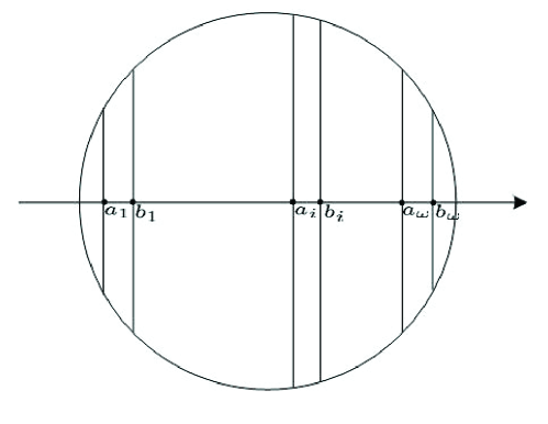
Figure 3: Example of $\left(r,y_{d-t+1},1+\frac{\epsilon_{4}}{g(d)}\right)$-Partitions in 2D

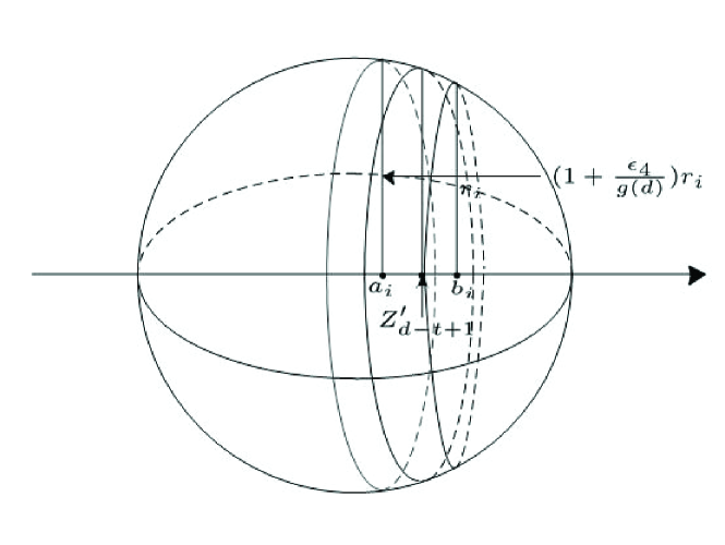
Figure 4: Example of $\left(r,y_{d-t+1},1+\frac{\epsilon_{4}}{g(d)}\right)$-Partitions in 3D

We have the following algorithm that can generate an approximate random lattice point in a large ball with an arbitrary center, which may not be a lattice point.

Definition 40

Let integer $d>0$ be a dimensional number, $\mathbb{R}^{d}$ be the $d-$dimensional Euclidean Space.

1. A point $q=(x^{\prime}_{1},x^{\prime}_{2},...,x^{\prime}_{d})\in\mathbb{R}^{d}$ is the nearest lattice point of $p=(x_{1},...,x_{d})\in\mathbb{R}^{d}$ if it satisfies $x^{\prime}_{i}=\left\{\begin{array}[]{rcl}\lfloor x_{i}\rfloor&&{x_{i}-[x_{i}]\leq\frac{1}{2}}\\ \lceil x_{i}\rceil&&{x_{i}-[x_{i}]>\frac{1}{2},}\end{array}\right.$ for $x_{i}\geq 0$ or $x^{\prime}_{i}=\left\{\begin{array}[]{rcl}\lceil x_{i}\rceil&&{|x_{i}|-[|x_{i}|]\leq\frac{1}{2}}\\ \lfloor x_{i}\rfloor&&{|x_{i}|-[|x_{i}|]<\frac{1}{2},}\end{array}\right.$ for $x_{i}<0,$ where $i=1,2,...,d.$

Algorithm 6 BigBallRandomLatticePoint(r, p, d)

$\mathbf{Input:}$ $p=(x_{1},\cdots,...,x_{d})$ where $x_{i}\in\mathbb{R}$ with $1\leq i\leq d,$ $\alpha\in(0,1)$ is a parameter to control the bias, $r$ is radius, and $k$ is dimensional number.
$\mathbf{Output:}$ Generate a random lattice point inside $d-$dimensional ball.

1:  Let $q$ be the nearest lattice point of $p$ in $\mathbb{R}^{d}$

2:  Repeat

3:    Let $s=$RecursiveBigBallRandomLatticePoint$(r+\sqrt{d},q,d)$

4:  Until $s\in B_{d}(r,p,d)$

5:  Return $s$

Theorem 41

For an arbitrary $\alpha\in(0,1),$ there is an algorithm with runing time ${\rm O}\left(\frac{d^{3}\log r}{\alpha}\right)$ and $(1+\alpha)-$bias for a $d-$dimensional ball $B_{d}(r,q,d)$ to generate a random lattice point with radius $r>\frac{2d^{3}}{\alpha}$ that centered at $q=(y_{1},y_{2},...,y_{d})$ with $y_{t}\in\mathbb{Z},$ $t=1,2,...,d.$

Proof:  In line 5 of algorithm RecursiveBigBallRandomLatticePoint(.), define

$r^{\prime 2}_{i}=\left\{\begin{array}[]{rcl}r^{2}-(y_{d-t+1}-a_{i})^{2}&&{if\ a_{i}\leq y_{d-t+1}}\\ r^{2}-(y_{d-t+1}-b_{i})^{2}&&{otherwise,}\end{array}\right.$,

$p^{\prime}_{i}=\left\{\begin{array}[]{rcl}(z_{1},z_{2},...,z_{d-t},a_{i},y_{d-t+2},...,y_{d})&&{if\ a_{i}\leq y_{d-t+1}}\\ (z_{1},z_{2},...,z_{d-t},b_{i},y_{d-t+2},...,y_{d})&&{otherwise,}\end{array}\right.$

and

$r^{2}_{i}=\left\{\begin{array}[]{rcl}r^{2}-(y_{d-t+1}-b_{i})^{2}&&{if\ b_{i}\leq y_{d-t+1}}\\ r^{2}-(y_{d-t+1}-a_{i})^{2}&&{otherwise,}\end{array}\right.$

$p_{i}=\left\{\begin{array}[]{rcl}(z_{1},z_{2},...,z_{d-t},b_{i},y_{d-t+2},...,y_{d})&&{if\ b_{i}\leq y_{d-t+1}}\\ (z_{1},z_{2},...,z_{d-t},a_{i},y_{d-t+2},...,y_{d})&&{otherwise.}\end{array}\right.$

Let $v(i)=(b_{i}-a_{i}+1),$ and $r^{\prime}_{i}=\frac{r_{i}}{1+\frac{\epsilon_{4}}{g(d)}},$ then we have

$$\sum\limits_{i}C(r^{\prime}_{i},p^{\prime}_{i},t-1)v(i)\leq C(r_{i},p_{i},t)\leq\sum\limits_{i}C(r_{i},p_{i},t-1)v(i).$$

Since $r^{\prime}_{i}=\frac{r_{i}}{1+\frac{\epsilon_{4}}{g(d)}},$ then

$$\frac{1-\beta}{1+\beta}\left(1+\frac{\epsilon_{4}}{g(d)}\right)^{-(t-1)}\sum\limits_{i}C(r_{i},p_{i},t-1)v(i)\leq C(r_{i},p_{i},t)$$

and

$$C(r_{i},p_{i},t)\leq\sum\limits_{i}C(r_{i},p_{i},t-1)v(i)$$

via Lemma 38, where $\delta=1+\frac{\epsilon_{4}}{g(d)}$.

Via Lemma 37 we have

$$\left(\frac{1-\beta}{1+\beta}\right)^{2}\left(1+\frac{\epsilon_{4}}{g(d)}\right)^{-(t-1)}\sum\limits_{i}P(r_{i},p_{i},t-1)v(i)\leq P(r_{i},p_{i},t)$$

and

$$P(r_{i},p_{i},t)\leq\frac{1+\beta}{1-\beta}\sum\limits_{i}P(r_{i},p_{i},t-1)v(i).$$

Thus, we have

$$\left(\frac{1-\beta}{1+\beta}\right)^{2}\left(1+\frac{\epsilon_{4}}{g(d)}\right)^{-(t-1)}\leq\frac{P(r_{i},p_{i},t)}{\sum\limits_{i}P(r_{i},p_{i},t-1)v(i)}\leq\frac{1+\beta}{1-\beta}.$$

From above inequality, we have

$$\left(\frac{1-\beta}{1+\beta}\right)^{2}\left(1+\frac{\epsilon_{4}}{g(d)}\right)^{-(t-1)}\frac{1}{P(r_{i},p_{i},t)}\leq\frac{1}{\sum\limits_{i}P(r_{i},p_{i},t-1)v(i)}\leq\frac{1+\beta}{1-\beta}\frac{1}{P(r_{i},p_{i},t)}.$$

Via Lemma 37 we have

$$\frac{(1-\beta)^{2}}{(1+\beta)^{3}}\left(1+\frac{\epsilon_{4}}{g(d)}\right)^{-(t-1)}\frac{1}{C(r_{i},p_{i},t)}\leq\frac{1}{\sum\limits_{i}P(r_{i},p_{i},t-1)v(i)}\leq\frac{1+\beta}{(1-\beta)^{2}}\frac{1}{C(r_{i},p_{i},t)}.$$

Let $g(d)=d^{2},$ $\epsilon_{4}=\frac{\alpha}{4}$ and $\beta=\frac{\alpha}{\alpha+16d+16}$. Since Algorithm RecursiveBigBallRandomLatticePoint(.) has $d$ iteration, we can generate a random lattice point with bias of probability as:

$$\frac{P(r_{i},p_{i},d-1)}{\sum\limits_{i}P(r_{i},p_{i},d-2)v(i)}\cdot\frac{P(r_{i},p_{i},d-2)}{\sum\limits_{i}P(r_{i},p_{i},d-1)v(i)}\cdots\frac{P(r_{i},p_{i},0)}{\sum\limits_{i}P(r_{i},p_{i},0)v(i)}$$

$$\leq \frac{1+\beta}{(1-\beta)^{2}}\frac{1}{C(r,p,d)}\cdot\left(\frac{1+\beta}{1-\beta}\right)^{d-1}\cdot P(r_{i},p_{i},0)$$

$$\leq \frac{1}{1-\beta}\frac{1}{C(r,p,d)}\cdot\left(\frac{1+\beta}{1-\beta}\right)^{d}\cdot(1+\beta)C(r_{i},p_{i},0)$$

$$= \left(\frac{1+\beta}{1-\beta}\right)^{d+1}\frac{1}{C(r,p,d)}$$

$$= \left(1+\frac{2\beta}{1-\beta}\right)^{d+1}\frac{1}{C(r,p,d)}$$

$$\leq e^{\frac{2\beta}{1-\beta}(d+1)}\frac{1}{C(r,p,d)}$$

$$\leq \left(1+\frac{4\beta}{1-\beta}(d+1)\right)\frac{1}{C(r,p,d)}$$

$$\leq (1+\alpha)\frac{1}{C(r,p,d)}$$

and

$$\frac{P(r_{i},p_{i},d-1)}{\sum\limits_{i}P(r_{i},p_{i},d-2)v(i)}\cdot\frac{P(r_{i},p_{i},d-2)}{\sum\limits_{i}P(r_{i},p_{i},d-1)v(i)}\cdots\frac{P(r_{i},p_{i},0)}{\sum\limits_{i}P(r_{i},p_{i},0)v(i)}$$

$$\geq \frac{(1-\beta)^{2}}{(1+\beta)^{3}}\left(1+\frac{\epsilon_{4}}{g(d)}\right)^{-(d-1)}\frac{1}{C(r,p,d)}\left(\frac{1-\beta}{1+\beta}\right)^{2(d-1)}\left(1+\frac{\epsilon_{4}}{g(d)}\right)^{\frac{-(d-1)(d-2)}{2}}(1-\beta)C(r_{i},p_{i},0)$$

$$= \left(\frac{1-\beta}{1+\beta}\right)^{2d+1}\left(1+\frac{\epsilon_{4}}{g(d)}\right)^{\frac{-(d-1)d}{2}}\frac{1}{C(r,p,d)}$$

$$\geq \left(1-\frac{2\beta}{1+\beta}\right)^{2d+1}\left(1+\frac{\epsilon_{4}}{g(d)}\right)^{\frac{-d^{2}}{2}}\frac{1}{C(r,p,d)}$$

$$\geq \left(1-\frac{2\beta}{1+\beta}\right)^{2d}\left(1+\frac{\epsilon_{4}}{g(d)}\right)^{-d^{2}}\frac{1}{C(r,p,d)}$$

$$\geq \left(1-\frac{4\beta d}{1+\beta}\right)\left(1-\frac{\epsilon_{4}d^{2}}{g(d)}\right)\frac{1}{C(r,p,d)}$$

$$\geq \left(1-\frac{4\beta d}{1+\beta}\right)\left(1-\epsilon_{4}\right)\frac{1}{C(r,p,d)}$$

$$\geq \left(1-\frac{4\beta d}{1+\beta}-\epsilon_{4}\right)\frac{1}{C(r,p,d)}$$

$$\geq \left(1-\frac{4\beta d}{1+\beta}\right)\left(1-\epsilon_{4}\right)\frac{1}{C(r,p,d)}$$

$$\geq \left(1-\alpha\right)\frac{1}{C(r,p,d)}.$$

Therefore, we can generate a random lattice point with probability between

$$\left[\left(1-\alpha\right)\frac{1}{C(r,p,d)},\ \left(1+\alpha\right)\frac{1}{C(r,p,d)}\right].$$

In line 3 of algorithm RecursiveBigBallRandomLatticePoint(.), it forms a $\left(r,y_{d-t+1},1+\frac{\epsilon_{4}}{g(d)}\right)$-partition $I_{1},\cdots,I_{w}$ for $[\lceil{y_{d-t+1}-r}\rceil,\lfloor{y_{d-t+1}+r}\rfloor]\cap\mathbb{Z}$ and $[y_{d-t+1}+1,\lfloor{y_{d-t+1}+r}\rfloor]\cap\mathbb{Z}$. Then, there are at most $w$ number of $a_{i}$, where $w$ such that $\frac{r}{\left(1+\frac{\epsilon_{4}}{g(d)}\right)^{w}}\leq 1.$ Solving $w,$ we have $w\geq\frac{g(d)\log r}{\epsilon_{4}}.$ And there are $d$ iterations in algorithm RecursiveBigBallRandomLatticePoint(.).

Thus, the running time of the algorithm is ${\rm O}\left(\frac{g(d)\log r}{\epsilon_{4}}\cdot d\right)={\rm O}(\frac{d^{3}\log r}{\epsilon_{4}})={\rm O}\left(\frac{d^{3}\log r}{\alpha}\right).$         

$\mathbf{Remark:}$ We note that there are at most one $(t-1)-$dimensional ball of radius $r<\frac{2d^{3}}{\alpha}$ with center at a lattice point, where $t=1,2,...,d.$ For this case, we can apply Theorem 35 with $\beta=0.$

Theorem 42

For arbitrary $\alpha\in(0,1),$ and $\alpha^{\prime}\in(0,1),$ there is an $(1+\alpha^{\prime})-$bias algorithm with runing time ${\rm O}\left(\frac{d^{3}\log(r+\sqrt{d})}{\alpha}\right)$ for a $d-$dimensional ball $B_{d}(r,q,d)$ to generate a random lattice point of radius $r>\frac{2d^{\frac{3}{2}}}{\alpha}$ with an arbitrary center.

Proof:  Consider another ball $B_{d}(r^{\prime},q,d)$ of radius $r^{\prime}$ with lattice center $q=(y_{1},y_{2},...,y_{d})$ that contains ball $B_{d}(r,p,d)$ , where $r^{\prime}=r+\sqrt{d}.$ Let $V_{d}(r)$ be the volume of a $d-$dimensional ball with radius $r,$ then probability that a lattice point in $B_{d}(r^{\prime},q,d)$ belongs to $B_{d}(r,p,d)$ is at least $(1-\alpha){C(r,p,d)\over C(r^{\prime},p,d)}$.

Via Theorem 32, we have

$$\left\{\begin{array}[]{lr}\frac{1}{1+\beta}V_{d}(r)\leq C(r,p,d)\leq\frac{1}{1-\beta}V_{d}(r)&\\ \frac{1}{1+\beta}V_{d}(r+\sqrt{d})\leq C(r^{\prime},q,d)\leq\frac{1}{1-\beta}V_{d}(r+\sqrt{d}),&\end{array}\right.$$

then we have

$$\frac{1-\beta}{1+\beta}\frac{V_{d}(r)}{V_{d}(r+\sqrt{d})}\leq\frac{C(r,p,d)}{C(r^{\prime},p,d)}\leq\frac{1+\beta}{1-\beta}\frac{V_{d}(r)}{V_{d}(r+\sqrt{d})}.$$

The formula for a $d-dimensional$ ball of raduis $r$ is

$$V_{d}(r)=f(d)\cdot r^{d}$$

where $f(d)=\pi^{\frac{d}{2}}\Gamma\left(\frac{1}{2}d+1\right)^{-1}$ and $\Gamma(.)$ is Euler’s gamma function. Let $\beta=\frac{\alpha}{8+\alpha}$ and $\alpha>\frac{2d^{\frac{3}{2}}}{r+\sqrt{d}},$

$$(1-\alpha){C(r,p,d)\over C(r^{\prime},p,d)} \geq(1-\alpha)\frac{1-\beta}{1+\beta}\frac{f(d)\cdot r^{d}}{f(d)\cdot\left(r+\sqrt{d}\right)^{d}}$$

$$=(1-\alpha)\frac{1-\beta}{1+\beta}\left(1-\frac{\sqrt{d}}{r+\sqrt{d}}\right)^{d}$$

$$\geq(1-\alpha)\frac{1-\beta}{1+\beta}\left(1-\frac{d^{\frac{3}{2}}}{r+\sqrt{d}}\right)$$

$$\geq(1-\alpha)\left(1-\frac{2\beta}{1-\beta}\right)\left(1-\frac{d^{\frac{3}{2}}}{r+\sqrt{d}}\right)$$

$$\geq\left(1-\alpha-\frac{2\beta}{1-\beta}-\frac{d^{\frac{3}{2}}}{r+\sqrt{d}}\right).$$

Therefore, the probability a lattice point in $B_{d}(r^{\prime},q,d)$ belongs to $B_{d}(r,p,d)$ fails is at most $\left(\alpha+\frac{2\beta}{1-\beta}+\frac{d^{\frac{3}{2}}}{r+\sqrt{d}}\right),$ where $\left(\alpha+\frac{2\beta}{1-\beta}+\frac{d^{\frac{3}{2}}}{r+\sqrt{d}}\right)<1,$ which means the algorithm BigBallRandomLatticePoint(.) fails with small possibility.

The probability to generate a random lattic point in ball $B_{d}(r^{\prime},q,d)$ is in range of

$$\left[(1-\alpha)\frac{1}{C(r^{\prime},q,d)},(1+\alpha)\frac{1}{C(r^{\prime},q,d)}\right]$$

via Theorem 41. Then the bias to generate a random lattic point in ball $B_{d}(r,p,d)$ is $\frac{\Pr(p_{i})}{\sum_{i}\Pr(p_{i})},$ where $\Pr(p_{i})\in\left[(1-\alpha)\frac{1}{C(r^{\prime},q,d)},(1+\alpha)\frac{1}{C(r^{\prime},q,d)}\right].$

Then, we have

$$\frac{\Pr(p_{i})}{\sum\limits_{i}\Pr(p_{i})} \leq\frac{(1+\alpha)\frac{1}{C(r^{\prime},q,d)}}{(1-\alpha)\frac{1}{C(r^{\prime},q,d)}C(r,p,d)}$$

$$=\frac{1+\alpha}{1-\alpha}\frac{1}{C(r,p,d)}$$

$$=\left(1+\frac{2\alpha}{1-\alpha}\right)\frac{1}{C(r,p,d)},$$

and

$$\frac{\Pr(p_{i})}{\sum\limits_{i}\Pr(p_{i})} \geq\frac{(1-\alpha)\frac{1}{C(r^{\prime},q,d)}}{(1+\alpha)\frac{1}{C(r^{\prime},q,d)}C(r,p,d)}$$

$$=\frac{1-\alpha}{1+\alpha}\frac{1}{C(r,p,d)}$$

$$=\left(1-\frac{2\alpha}{1+\alpha}\right)\frac{1}{C(r,p,d)}$$

$$\geq\left(1-\frac{2\alpha}{1-\alpha}\right)\frac{1}{C(r,p,d)}.$$

Therefore, the probability to generate a random lattice point in $B_{d}(r,p,d)$ is range of

$$\left[(1-\alpha^{\prime})\frac{1}{C(r,p,d)},(1+\alpha^{\prime})\frac{1}{C(r,p,d)}\right]$$

where $\alpha^{\prime}=\frac{2\alpha}{1-\alpha}.$

It takes ${\rm O}\left(\frac{d^{3}\log(r+\sqrt{d})}{\alpha}\right)$ running time to generate a random lattice point inside a $d-$dimensional ball $B_{d}(r+\sqrt{d},p,d)$ with a lattice point center via Theorem 41. Thus, the algorithm BigBallRandomLatticePoint(.) takes ${\rm O}\left(\frac{d^{3}\log(r+\sqrt{d})}{\alpha}\right)$ running time to generate a random lattice.         

Theorem 43

For an arbitrary $\alpha\in(0,1),$ there is an algorithm with runing time ${\rm O}\left(\frac{d^{3}\log(r+\sqrt{d})}{\alpha}\right)$ and $(1+\alpha)-$bias for a $d-$dimensional ball $B_{d}(r,q,d)$ to generate a random lattice pointo f radius $r>\frac{2d^{\frac{3}{2}}}{\alpha}$ with a arbitrary center; and there is a ${\rm O}\left(\frac{1}{\beta}d^{\frac{11}{2}}l^{3}\left(\frac{2d^{\frac{3}{2}}}{\beta}+l|\lambda|\right)^{3}\right)$ time algorithm to generate a lattice point inside a $d-$dimensional ball $B_{d}(r,p,d)$ of radius $r\leq\frac{2d^{\frac{3}{2}}}{\alpha}$ with center $p\in D(\lambda,d,l)$.

Proof:  We discuss two cases based the radius of the $d$-dimensional ball.

Case 1: When generate a random lattice point inside a $d$-dimensional ball of radius $r>\frac{2d^{\frac{3}{2}}}{\alpha}$ with center arbitrary center $p$, apply Theorem  42.

Case 2: When generate a random lattice point inside a $d$-dimensional ball of radius $r\leq\frac{2d^{\frac{3}{2}}}{\alpha}$ with center $p\in D(\lambda,d,l)$, apply Theorem  35.         

5.3 Count Lattice Point in the Union of High Dimensional Balls

In this section, we apply the algorithm developed in Section 4 to count the total number of lattice point in the union of high dimensional balls.

Theorem 44

There is a ${\rm O}\left({\rm poly}\left({1\over\epsilon},\log{1\over\gamma}\right)\cdot{m}\cdot(\log{m})^{{\rm O}(1)}\right)$ time and ${\rm O}(\log m)$ rounds algorithm for the number of lattice points in $B_{1}\cup B_{2}\cup\cdots\cup B_{m}$ such that with probability at least $1-\gamma$, it gives a $sum\cdot M\in[{(1-\epsilon)(1-\alpha_{L})(1-\beta_{L})}\cdot|B_{1}\cup\cdots\cup B_{m}|,{(1+\epsilon)(1+\alpha_{R})(1+\beta_{R})}\cdot|B_{1}\cup\cdots\cup B_{m}|],$ where each ball $B_{i}$ satisfy that either its radius $r>\frac{2d^{\frac{3}{2}}}{\beta}$ or its center $p\in D(\lambda,d,l)$ and $|B_{1}\cup\cdots\cup B_{m}|$ is the total number of lattice point of union of $m$ high dimensional balls.

Proof:  Apply Theorem 33 and Theorem 43, we have $m_{i}$ for each ball $B_{i}$ with

$$m_{i}\in\left((1-\beta_{L})C_{i}(r_{i},p_{i},t),(1+\beta_{R})C_{i}(r_{i},p_{i},t)\right),$$

and biased random generators with

$${\rm Prob}(x={\rm RandomElement}(B_{i}))\in\left[{1-\alpha_{L}\over C_{i}(r_{i},p_{i},t)},{1+\alpha_{R}\over C_{i}(r_{i},p_{i},t)}\right]$$

for each input ball $B_{i}$, where $C_{i}(r_{i},p_{i},t)$ is the number of lattice point of $t-$dimensional ball $B_{i}$ of radius $r_{i}$ for $i=1,2,...,m$. Then apply Theorem 17.         

5.4 Hardness to Count Lattice Points in a Set of Balls

In this section, we show that it is #P-hard to count the number of lattice points in a set of balls.

Theorem 45

It is #P-hard to count the number of lattice points in a set of $d$-dimensional balls even the centers are of the format $(x_{1},\cdots,x_{d})\in\mathbb{R}^{d}$ that has each $x_{i}$ to be either $1$ or ${\sqrt{h}\over 2}$ for some integer $h\leq d$.

Proof:  We derive a polynomial time reduction from DNF problem to it. For each set of lattice points in a $h$-dimensional cube $\{0,1\}^{h}$, we design a ball with radius $r={\sqrt{h}\over 2}$ and center at $C=({\sqrt{h}\over 2},\cdots,{\sqrt{h}\over 2})$. It is easy to see that this ball only covers the lattice points in $\{0,1\}^{h}$. Every $0,1$-lattice point in ${0,1}$ has distance to the center $C$ equal to $r$. For every lattice point $P\in R^{h}$ that is not in $\{0,1\}^{h}$ has distance $d$ with $d^{2}\geq r^{2}+(1+{1\over 2})^{2}-({1\over 2})^{2}=r^{2}+2$.         

Definition 46

For a center $c=(c_{1},\cdots,c_{d})$ and an even number $k>0$ and a real $r>0$, a $d$-dimensional $k$-degree ball $B_{k}(c,r)$ is $\{(x_{1},\cdots,x_{d}):(x_{1},\cdots,x_{d})\in\mathbb{R}^{d}$ and $\sum\limits_{i=1}^{d}(x_{i}-c_{i})^{k}\leq r\}$.

Theorem 47

Let $k$ be an even number at least $2$. Then we have:

1. There is no polynomial time algorithm to approximate the number of lattice points in the intersection $n$-dimensional $k$-degree balls unless P=NP.

2. It is #P-hard to count the number of lattice points in the intersection $n$-dimensional $k$-degree balls.

Proof:  We derive a polynomial time reduction from 3SAT problem to it. For each clause $C=(x_{i}^{*}\vee x_{j}^{*}\vee x_{k}^{*})$, we can get a ball to contain all lattice points in the 0-1-cube to satisfy $C$, each $x_{i}^{*}$ is a literal to be either $x_{i}$ or its negation $\bar{x_{i}}$.

Without loss of generality, let $C=(x_{1}\vee x_{2}\vee x_{3})$. Let $\delta=0.30$. Let center $D_{C}=(d_{1},d_{2},d_{3},d_{4},d_{5},\cdots,d_{n})=(1-\delta,1-\delta,1-\delta,{1\over 2},{1\over 2},\cdots,{1\over 2})$, which has value $1-\delta$ in the first three positions, and ${1\over 2}$ in the rest. For $0,1$ assignment $(a_{1},a_{2},\cdots,a_{n})$ of $n$ variables, if it satisfies $C$ if and only if $\sum\limits_{i=1}^{n}(a_{i}-d_{i})^{k}\leq 2(1-\delta)^{k}+\delta^{k}+(n-3)\cdot({1\over 2})^{k}$. Therefore, we can select radius $r_{C}$ that satisfies $r_{C}^{k}=2(1-\delta)^{k}+\delta^{k}+(n-3)\cdot({1\over 2})^{k}$. We have the following inequalities:

$$\left\{\begin{array}[]{lr}(2-\delta)^{2}>(1+\delta)^{k}>2(1-\delta)^{k}+\delta^{k}\\ (1+{1\over 2})^{k}>2(1-\delta)^{k}+\delta^{k}+({1\over 2})^{k}.\end{array}\right.$$ (49)

This is because we have the following equalities:

$$\left\{\begin{array}[]{lr}(1+\delta)^{2}=1.69,\\ 2(1-\delta)^{2}+\delta^{2}=2\times 0.49+0.09=1.07,\\ 2(1-\delta)^{2}+\delta^{2}+({1\over 2})^{2}=1.07+0.25=1.32,\\ (1+{1\over 2})^{2}=2.25.\end{array}\right.$$ (50)

If $Y=(y_{1},y_{2},\cdots,y_{n})$ is not a $0,1$-lattice point, we discuss two cases:

1. Case 1. $y_{i}\not\in\{0,1\}$ for some $i$ with $1\leq i\leq 3$.

   In this case we know that dist$(Y,D_{C})^{2}>r_{C}^{2}$ by inequality (50).

2. Case 2. $y_{i}\not\in\{0,1\}$ for some $i$ with $3<i\leq n$.

   In this case we know that dist$(Y,D_{C})^{2}>r_{C}^{2}$ by inequality (50).

If $Y=(y_{1},y_{2},\cdots,y_{n})$ is a $0,1$-lattice point, we discuss two cases:

1. Case 1. $Y$ satisfies $C$.

   In this case we know that dist$(Y,D_{C})^{2}\leq r_{C}^{2}$.

2. Case 2. $Y$ does not satisfy $C$.

   In this case we know that dist$(Y,D_{C})^{2}>r_{C}^{2}$ by inequality $(1-\delta)^{2}>\delta^{2}$.

The ball $B_{C}$ with center at $D_{C}$ and radius $r_{C}$ contains exactly those 0,1-lattice points that satisfy clause $C$. This proves the first part of the theorem.

If there were any factor $c$-approximation to the intersection of balls, it would be able to test if the intersection is empty. This would bring a polynomial time solution to 3SAT.

It is well known that #3SAT is #P-hard. Therefore, It is #P-hard to count the number of lattice points in the intersection $n$-dimensional balls. This proves the second part of the theorem.

 

6 Approximation for the Maximal Coverage with Balls

We apply the technology developed in this paper to the maximal coverage problem when each set is a set of lattice points in a ball with center in $D(\lambda,d,l)$.

The classical maximum coverage is that given a list of sets $A_{1},\cdots,A_{m}$ and an integer $k$, find $k$ sets from $A_{1},A_{2},\cdots,A_{m}$ to maximize the size of the union of the selected sets in the computational model defined in Definition 2. For real number $a\in[0,1]$, an approximation algorithm is a $(1-a)$-approximation for the maximum coverage problem that has input of integer parameter $k$ and a list of sets $A_{1},\cdots,A_{m}$ if it outputs a sublist of sets $A_{i_{1}},A_{i_{2}},\cdots,A_{i_{k}}$ such that $|A_{i_{1}}\cup A_{i_{2}}\cup\cdots\cup A_{i_{k}}|\geq(1-a)|A_{j_{1}}\cup A_{j_{2}}\cup\cdots\cup A_{j_{k}}|$, where $A_{j_{1}},A_{j_{2}},\cdots,A_{j_{k}}$ is a solution with maximum size of union.

Theorem 48

[17] Let $\rho$ be a constant in $(0,1)$. For parameters $\xi,\gamma\in(0,1)$ and $\alpha_{L},\alpha_{R},\delta_{L},\delta_{R}\in[0,1-\rho]$, there is an algorithm to give a $\left(1-(1-{\beta\over k})^{k}-\xi\right)$-approximation for the maximum cover problem, such that given a $((\alpha_{l},\alpha_{r}),(\delta_{L},\delta_{R}))$-list $L$ of finite sets $A_{1},\cdots,A_{m}$ and an integer $k$, with probability at least $1-\gamma$, it returns an integer $z$ and a subset $H\subseteq\{1,2,\cdots,m\}$ that satisfy

1. $|\cup_{j\in H}A_{j}|\geq\left(1-(1-{\beta\over k})^{k}-\xi\right)C^{*}(L,k)$ and $|H|=k$,

2. $((1-\alpha_{L})(1-\delta_{L})-\xi)|\cup_{j\in H}A_{j}|\leq z\leq((1+\alpha_{R})(1+\delta_{R})+\xi)|\cup_{j\in H}A_{j}|$, and

3. Its complexity is $(T(\xi,\gamma,k,m),R(\xi,\gamma,k,m),Q(\xi,\gamma,k,m))$ with

   $$T(\xi,\gamma,k,m) = {\rm O}\left({k^{3}\over\xi^{2}}\left(k\log\left({3m\over k}\right)+\log{1\over\gamma}\right)m\right),$$

   where $\beta={(1-\alpha_{L})(1-\delta_{L})\over(1+\alpha_{R})(1+\delta_{R})}$ and $C^{*}(L,k)$ is the number of elements to be covered in an optimal solution.

We need Lemma 49 to transform the approximation ratio given by Theorem 48 to constant $(1-{1\over e})$ to match the classical ratio for the maximum coverage problem.

Lemma 49

For each integer $k\geq 2$, and real $b\in[0,1]$, we have:

1. $(1-{b\over k})^{k}\leq{1\over e}-{\eta\over e}(b+{b\over 2k}-1)$.

2. If $\xi\leq{\eta\over e}(b+{b\over 2k}-1)$, then $1-(1-{b\over k})^{k}-\xi>1-{1\over e}$, where $\eta=e^{-{1\over 4}}$.

Proof: Let function $f(x)=1-\eta x-e^{-x}$. We have $f(0)=0$. Taking differentiation, we get ${df(x)\over dx}=-\eta+e^{-x}>0$ for all $x\in(0,{1\over 4})$.

Therefore, for all $x\in(0,{1\over 4})$,

$$e^{-x}\leq 1-\eta x.$$ (51)

The following Taylor expansion can be found in standard calculus textbooks. For all $x\in(0,1)$,

$$\ln(1-x)=-x-{x^{2}\over 2}-{x^{3}\over 3}-\cdots.$$

Therefore, we have

$$(1-{b\over k})^{k} = e^{k\ln(1-{b\over k})}=e^{k(-{b\over k}-{b^{2}\over 2k^{2}}-{b^{3}\over 3k^{3}}-\cdots)}=e^{-b-{b^{2}\over 2k}-{b^{3}\over 3k^{2}}-\cdots}$$ (52)

$$\leq e^{-b-{b\over 2k}}=e^{-1}\cdot e^{1-b-{b\over 2k}}$$

$$\leq e^{-1}\cdot(1-\eta\cdot(b+{b\over 2k}-1))\leq{1\over e}-{\eta\over e}(b+{b\over 2k}-1).$$ (53)

Note that the transition from (52) to (53) is based on inequality (51).

The part ii follows from part i. This is because $1-(1-{b\over k})^{k}-\xi\geq 1-{1\over e}+{\eta\over e}(b+{b\over 2k}-1)-\xi\geq 1-{1\over e}$.         

Theorem 50

There is a poly$(\lambda,d,l,k,m)$ time $(1-{1\over e})$-approximation algorithm for maximal coverage problem when each set is the set of lattice points in a ball with center in $D(\lambda,d,l)$.

Proof: [Sketch] Let $\alpha=\alpha_{L}=\alpha_{R}=\delta_{L}=\delta_{R}={1\over ck}$ with $c=100$, and $b=\beta={1-\alpha_{L})(1-\delta_{L})\over(1+\alpha_{R})(1+\delta_{R})}$. It is easy to see $(b+{b\over 2k}-1)\geq{1\over 4k}$. Let $\xi={\eta\over e}(b+{b\over 2k}-1)=\Theta({1\over k})$. It follows from Theorem 48, Lemma 49, Theorem 33 and Theorem 43.         

7 Conclusions

We introduce an almost linear bounded rounds randomized approximation algorithm for the size of set union problem $\arrowvert A_{1}\cup A_{2}\cup...\cup A_{m}\arrowvert$, which given a list of sets $A_{1},...,A_{m}$ with approximate set size and biased random generators. The definition of round is introduced. We prove that our algorithm runs sublinear in time under certain condition. A polynomial time approximation scheme is proposed to approximae the number of lattice points in the union of d-dimensional ball if each ball center satisfy $D(\lambda,d,l)$. We prove that it is $\#$P-hard to count the number of lattice points in a set of balls, and we also show that there is no polynomial time algorithm to approximate the number of lattice points in the intersection of $n$-dimenisonal $k$-degree balls unless P=NP.

8 Acknowledgements

We want to thank Peter Shor, Emil Je$\check{r}\acute{a}$bek, Rahul Savani et al. for their comments about algorithm to geneate a random grid point inside a $d-$dimensional ball on Theoretical Computer Science Stack Exchange.

References

- [1] S. D. Adhikari and Y. F. S. Ptermann. Lattice points in ellipsoids. Acta Arith., 59(4):329–338, 1991.
- [2] N. Alon, Y. Matias, and M. Szegedy. The space complexity of approximating the frequency moments. In Proceedings of the Twenty-Eighth Annual ACM Symposium on the Theory of Computing, Philadelphia, Pennsylvania, USA, May 22-24, 1996, pages 20–29, 1996.
- [3] G. E. Andrews, S. B. Ekhad, and D. Zeilberger. A short proof of jacobi’s formula for the number of representations of an integer as a sum of four squares. The American Mathematical Monthly, Vol. 100, No. 3:274–276, 1993.
- [4] Z. Bar-Yossef, T. S. Jayram, R. Kumar, D. Sivakumar, and L. Trevisan. Counting distinct elements in a data stream. In Randomization and Approximation Techniques, 6th International Workshop, RANDOM 2002, Cambridge, MA, USA, September 13-15, 2002, Proceedings, pages 1–10, 2002.
- [5] Z. Bar-Yossef, R. Kumar, and D. Sivakumar. Reductions in streaming algorithms, with an application to counting triangles in graphs. In Proceedings of the Thirteenth Annual ACM-SIAM Symposium on Discrete Algorithms, January 6-8, 2002, San Francisco, CA, USA., pages 623–632, 2002.
- [6] J. Beck. On a lattice point problem of l. moser I. Combinatorica, 8(1):21–47, 1988.
- [7] J. Blasiok. Optimal streaming and tracking distinct elements with high probability. In Proceedings of the Twenty-Ninth Annual ACM-SIAM Symposium on Discrete Algorithms, SODA 2018, New Orleans, LA, USA, January 7-10, 2018, pages 2432–2448, 2018.
- [8] K. Bringmann and T. Friedrich. Approximating the volume of unions and intersections of high-dimensional geometric objects. Comput. Geom., 43(6-7):601–610, 2010.
- [9] S. R. Buss and L. Hay. On truth-table reducibility to SAT and the difference hierarchy over NP. In Proceedings: Third Annual Structure in Complexity Theory Conference, Georgetown University, Washington, D. C., USA, June 14-17, 1988, pages 224–233, 1988.
- [10] K. Chandrasekharan and R. Narasimhan. On lattice-points in a random sphere. Bull. Amer. Math. Soc., 73(1):68–71, 1967.
- [11] J.-R. Chen. Improvement on the asymptotic formulas for the number of lattice points in a region of the three dimensions (ii). Scientia Sinica, 12(5).
- [12] S. A. Cook. The complexity of theorem-proving procedures. In Proceedings of the 3rd Annual ACM Symposium on Theory of Computing, May 3-5, 1971, Shaker Heights, Ohio, USA, pages 151–158, 1971.
- [13] K. Corradi and I. Ktai. A comment on k. s. gangadharan’s paper entitled ”two classical lattice point problems”. Magyar Tud. Akad. Mat. Fiz. Oszt. Kozl, 17.
- [14] P. Flajolet, É. Fusy, O. Gandoue, and F. Meunier. Hyperloglog: the analysis of a near-optimal cardinality estimation algorithm. In 2007 Conference on Analysis of Algorithms, AofA 07, pages 127–146, 2007.
- [15] P. Flajolet and G. N. Martin. Probabilistic counting algorithms for data base applications. J. Comput. Syst. Sci., 31(2):182–209, 1985.
- [16] L. Fortnow and N. Reingold. PP is closed under truth-table reductions. In Proceedings of the Sixth Annual Structure in Complexity Theory Conference, Chicago, Illinois, USA, June 30 - July 3, 1991, pages 13–15, 1991.
- [17] B. Fu. Partial sublinear time approximation and inapproximation for maximum coverage. arXiv:1604.01421, April 5, 2016.
- [18] S. Ganguly, M. N. Garofalakis, and R. Rastogi. Tracking set-expression cardinalities over continuous update streams. VLDB J., 13(4):354–369, 2004.
- [19] P. B. Gibbons. Distinct sampling for highly-accurate answers to distinct values queries and event reports. In VLDB 2001, Proceedings of 27th International Conference on Very Large Data Bases, September 11-14, 2001, Roma, Italy, pages 541–550, 2001.
- [20] P. B. Gibbons and S. Tirthapura. Estimating simple functions on the union of data streams. In SPAA, pages 281–291, 2001.
- [21] P. J. Haas, J. F. Naughton, S. Seshadri, and L. Stokes. Sampling-based estimation of the number of distinct values of an attribute. In VLDB’95, Proceedings of 21th International Conference on Very Large Data Bases, September 11-15, 1995, Zurich, Switzerland., pages 311–322, 1995.
- [22] J. L. Hafner. New omega theorems for two classical lattice point problems. Inventiones Mathematicae, 63(2):181–186, 1981.
- [23] D. R. Heath-Brown. Lattice points in sphere. Numb. Theory Prog., 2:883–892, 1999.
- [24] W. Hoeffding. Probability inequalities for sums of bounded random variables. Journal of the American Statistical Association, 58(301):13–30, 1963.
- [25] Z. Huang, W. M. Tai, and K. Yi. Tracking the frequency moments at all times. CoRR, abs/1412.1763, 2014.
- [26] M. N. Huxley. Exponential sums and lattice points ii. Proc. London Math. Soc., 66(2):279–301, 1993.
- [27] C. Jacobi. Gesammelte Werke, Berlin 1881-1891. Reprinted by Chelsea, New York, 1969.
- [28] D. M. Kane, J. Nelson, and D. P. Woodruff. An optimal algorithm for the distinct elements problem. In Proceedings of the Twenty-Ninth ACM SIGMOD-SIGACT-SIGART Symposium on Principles of Database Systems, PODS 2010, June 6-11, 2010, Indianapolis, Indiana, USA, pages 41–52, 2010.
- [29] R. M. Karp, M. Luby, and N. Madras. Monte-carlo approximation algorithms for enumeration problems. J. Algorithms, 10(3):429–448, 1989.
- [30] J. E. Mazo and A. M. Odlyzko. Lattice points in high-dimensional spheres. Monatsh. Math., 110(1):47–61, 1990.
- [31] A. Meyer. On the number of lattice points in a small sphere and a recursive lattice decoding algorithm. Des. Codes Cryptography, 66(1-3):375–390, 2013.
- [32] R. Motwani and P. Raghavan. Randomized Algorithms. Cambridge University Press, 2000.
- [33] G. Szeg. Beitrge zur theorie der laguerreschen polynome ii: Zahlentheoretische anwendungen. Math. Z., 25(1).
- [34] K.-M. Tsang. Counting lattice points in the sphere. Bulletin of the London Mathematical Society, 32(6).
- [35] L. G. Valiant. The complexity of computing the permanent. Theor. Comput. Sci., 8:189–201, 1979.
- [36] A. I. Vinogradov and M. M. Skriganov. The number of lattice points inside the sphere with variable cente, analytic number theory and the theory of functions, 2. Zap. Nauen. Sem. Leningrad Otdel. Mat. Inst. Steklov (LOMI), 91:25–30, 1979.
- [37] I. M. Vinogradov. On the number of integer points in a sphere. Izu. Akad. Nauk SSSR Ser. Mat., 27(5):957–968, 1963.
- [38] A. Walfisz. Gitterpunkte in mehrdimensionalen Kugeln. Instytut Matematyczny Polskiej Akademi Nauk(Warszawa), 1957.
- [39] A. Walfisz. Weylsche exponentialsummen in der neueren zahlentheorie. VEB Deutscher Verlag der Wissenschaften, 1963.
- [40] A. A. Yudin. On the number of integer points in the displaced circles. Acta Arith, 14(2):141–152, 1968.