Numerical solution of boundary value problems for the eikonal equation in an anisotropic medium

Abstract

A Dirichlet problem is considered for the eikonal equation in an anisotropic medium. The nonlinear boundary value problem (BVP) formulated in the present work is the limit of the diffusion–reaction problem with a diffusion parameter tending to zero. To solve numerically the singularly perturbed diffusion–reaction problem, monotone approximations are employed. Numerical examples are presented for a two-dimensional BVP for the eikonal equation in an anisotropic medium. The standard piecewise-linear finite-element approximation in space is used in computations.

1 Introduction

Many applied problems lead to the need of solving a BVP for the eikonal equation. First of all, this nonlinear partial differential equation is used to simulate wave propagation in the approximation of geometric optics [1, 2]. In computational fluid dynamics, image processing and computer graphics (see, for example, [3, 4]), the solution of BVPs for the eikonal equation is associated with calculating the nearest distance to boundaries of a computational domain.

The eikonal equation is a typical example of steady-state Hamilton–Jacobi equations. The issues of the existence and uniqueness of the solution for boundary value problems for such equations are considered, e.g., in [5, 6]. To solve numerically BVPs for the eikonal equation, the standard approaches are used, which are based on using difference methods on rectangular grids or finite-element/finite-volume approximations on general irregular grids. In this approach, the main attention is paid to problems of nonlinearity.

A boundary value problem is formulated in the following way. The function $u(\bm{x})$ is defined as the solution of the equation

$$|\nabla u|^{2}=1,\quad\bm{x}\in\Omega$$ (1)

in a domain $\Omega$ with the specified boundary conditions

$$u(\bm{x})=0,\quad\bm{x}\in\partial\Omega.$$ (2)

Computational algorithms for solving BVPs for the eikonal equation can be divided into two classes.

Marching methods (the first class of algorithms) are the most widely used. They are based on the hyperbolic nature of the eikonal equation. In this case, the desired solution of the problem (1), (2) is obtained by successive moving into the interior of the domain from its boundary, using, for instance, first-order upwind finite differences [7, 8]. Among other popular methods, we should mention, first of all, the fast sweeping method [9, 10], which uses a Gauss–Seidel-style update strategy to progress across the domain. Recently (see, for example, [11]), a fast iterative method for eikonal equations is actively developed using triangular [12] and tetrahedral [13] grids. Other modern variants of the fast marching method, which are adapted, in particular, to modern computing systems of parallel architecture, have been studied and compared, e.g., in [14].

The second class of algorithms is associated with a transition from (1), (2) to a linear or nonlinear BVP for an elliptic equation [15]. Instead of equation (1), we (see [16]) minimize the functional

$$J(u)=\frac{1}{2}\int_{\Omega}(|\nabla u|-1)^{2}d\bm{x}.$$

It is possible to solve the BVP for the Euler–Lagrange equation for this functional, which has the form

$$\triangle u-\nabla\cdot\left(\frac{\nabla u}{|\nabla u|}\right)=0,\quad\bm{x}\in\Omega.$$

In [17], the computational algorithm is based on solving the nonlinear boundary value problem for $v=1/u$. The solution of the problem (1), (2) can be related to the solution of the homogeneous Dirichlet problem for $p$-Laplacian:

$$\nabla\cdot(|\nabla u_{p}|^{p-2}\nabla u_{p})=-1,\quad\bm{x}\in\Omega.$$

In this case (see, e.g., [18, 19]), we have

$$u_{p}(\bm{x})\rightarrow u(\bm{x})\ \mathrm{as}\ p\rightarrow\infty,\quad\bm{x}\in\Omega.$$

Thus, to find the solution of the problem (1), (2), we need to solve the nonlinear BVPs.

In our study, we focus on solving auxiliary boundary value problems for linear equations. This approach (see [20, 21])is based on a connection between the nonlinear Hamilton–Jacobi equation and the linear Schrodinger equation. Let $v_{\alpha}(\bm{x})$ be the solution of the boundary value problem

$$-\alpha^{2}\triangle v_{\alpha}+v_{\alpha}=0,\quad\bm{x}\in\Omega,$$ (3)

$$v_{\alpha}(\bm{x})=1,\quad\bm{x}\in\partial\Omega.$$ (4)

Then, for $u_{\alpha}(\bm{x})=-\alpha\ln(v_{\alpha}(\bm{x})$, we have $u_{\alpha}(\bm{x})\rightarrow u(\bm{x})$ as $\alpha\rightarrow 0$. A similar approach, where the auxiliary functions $v_{\alpha}(\bm{x})$ are associated with the solution of the unsteady heat equation, is considered in the paper [22].

In the present paper, we consider the eikonal equation in an anisotropic medium that is a more general variant in comparison with (1). Using the transformation $u(\bm{x})=-\alpha\ln(v(\bm{x}))$, the corresponding BVP of type (3), (4) is formulated for the new unknown quantity. In our case, $\alpha\rightarrow 0$ and so, we have a singularly perturbed BVP for the diffusion–reaction equation [23, 24]. The numerical solution is based on using standard Lagrangian finite elements [25, 26]. The main attention is paid to the monotonicity of the approximate solution for the auxiliary problem.

The paper is organized as follows. A boundary value problem for the eikonal equation in an anisotropic medium is formulated in Section 2. Its approximate solution is based on a transition to a singularly perturbed diffusion–convection equation. In Section 3, an approximation in space is constructed using Lagrangian finite elements and the main features of the problem solution are discussed. Numerical experiments on the accuracy of the approximate solution are presented in Section 5 for model two-dimensional problems. The results of the work are summarized in Section 5.

2 Transformation of BVP for the eikonal equation in an anisotropic medium

In a bounded polygonal domain $\Omega\subset R^{m}$, $m=1,2,3$ with the Lipschitz continuous boundary $\partial\Omega$, we search the solution of the BVP for the eikonal equation

$$Eu=1,\quad\bm{x}\in\Omega.$$ (5)

Define the operator $E$ as

$$Eu=\sum_{i=1}^{m}a_{i}^{2}\left(\frac{\partial u}{\partial x_{i}}\right)^{2}$$ (6)

with the coefficients $a_{i}({\bm{x}})>0$. The equation (5) is supplemented with the homogeneous Dirichlet boundary condition

$$u({\bm{x}})=0,\quad{\bm{x}}\in\partial\Omega.$$ (7)

The basic problems of numerical solving the boundary value problem (1)–(3) result from the nonlinearity of the equation (see the operator $E$).

Similarly to [20, 21], we introduce the transformation

$$v_{\alpha}(\bm{x})=\exp\left(-\frac{u_{\alpha}(\bm{x})}{\alpha}\right)$$ (8)

with a numerical parameter $\alpha>0$. This type of transformation is widely used in studying differential equations with quadratic nonlinearity $Eu$ (see, e.g., [27]).

Define the elliptic second-order operator $L$ by the relation

$$Lu=\sum_{i=1}^{m}\frac{\partial}{\partial x_{i}}\left(a_{i}^{2}\frac{\partial u}{\partial x_{i}}\right).$$ (9)

For (8), we have

$$\begin{split}a_{i}^{2}\frac{\partial v_{\alpha}}{\partial x_{i}}=&-\frac{1}{\alpha}\exp\left(-\frac{u_{\alpha}(\bm{x})}{\alpha}\right)a_{i}^{2}\frac{\partial u_{\alpha}}{\partial x_{i}},\\ \frac{\partial}{\partial x_{i}}\left(a_{i}^{2}\frac{\partial v_{\alpha}}{\partial x_{i}}\right)=&-\frac{1}{\alpha}\exp\left(-\frac{u_{\alpha}(\bm{x})}{\alpha}\right)\frac{\partial}{\partial x_{i}}\left(a_{i}^{2}\frac{\partial u_{\alpha}}{\partial x_{i}}\right)\\ &+\frac{1}{\alpha^{2}}\exp\left(-\frac{u_{\alpha}(\bm{x})}{\alpha}\right)a_{i}^{2}\left(\frac{\partial u_{\alpha}}{\partial x_{i}}\right)^{2}.\end{split}$$

By virtue of this, we obtain

$$\alpha^{2}Lv_{\alpha}-v_{\alpha}=\exp\left(-\frac{u_{\alpha}(\bm{x})}{\alpha}\right)(Eu_{\alpha}-1-\alpha Lu_{\alpha}).$$

Let $u_{\alpha}(\bm{x})$ satisfies the equation

$$\alpha Lu_{\alpha}-Eu_{\alpha}=-1,\quad\bm{x}\in\Omega,$$ (10)

and the boundary conditions

$$u_{\alpha}({\bm{x}})=0,\quad{\bm{x}}\in\partial\Omega.$$ (11)

Under these conditions, for $v_{\alpha}(\bm{x})$, we have the equation

$$\alpha^{2}Lv_{\alpha}-v_{\alpha}=0,\quad\bm{x}\in\Omega.$$ (12)

In view of (8), from (11), we obtain the following boundary condition:

$$v_{\alpha}({\bm{x}})=1,\quad{\bm{x}}\in\partial\Omega.$$ (13)

The equation (10) can be treated as a regularization of the Hamilton–Jacobi equation via the method of vanishing viscosity [28]. The boundary value problem (10), (11) produces an approximate solution of the problem (5), (6) for small values of $\alpha$:

$$u_{\alpha}(\bm{x})\rightarrow u(\bm{x})\ \mathrm{as}\ \alpha\rightarrow 0,\quad\bm{x}\in\Omega.$$

In this case, $u_{\alpha}(\bm{x})$ is defined according to (8) from the solution of the linear boundary value problem (12), (13).

3 Numerical implementation

An approximate solution of the BVP (5)–(7) is represented (see (8)) in the form

$$u_{\alpha}(\bm{x})=-\alpha\ln(v_{\alpha}(\bm{x})),$$ (14)

at a sufficiently low value of $\alpha$. In this case, $v_{\alpha}(\bm{x})$ is defined as the solution of the BVP (12), (13). In the present work, the numerical implementation of this approach is carried out on the basis of standard finite-element approximations [25, 26]. The main features of the computational algorithm result from the fact that the BVP of diffusion–reaction (12), (13) at small $\alpha$ is singularly perturbed, i.e., we have a small parameter at higher derivatives [29, 30].

Let us consider a standard quasi-uniform triangulation of the domain $\Omega$ into triangles in the 2D case or tetrahedra for 3D case. Let

$$V_{0}=\{v\in H^{1}(\Omega)\ |\ v(\bm{x})=0,\ \bm{x}\in\partial\Omega\},$$

$$V_{1}=\{v\in H^{1}(\Omega)\ |\ v(\bm{x})=1,\ \bm{x}\in\partial\Omega\}.$$

Denote by $V^{h}_{0}\subset V_{0}$ and $V^{h}_{1}\subset V_{1}$ the linear finite-element spaces.

For the BVP (12), (13), we put into the correspondence the variational problem of finding the numerical solution $y\in V^{h}_{1}$ from the conditions

$$a(y,v)=0,\quad\forall v\in V^{h}_{0}.$$ (15)

By (9), for the bilinear form, we have

$$a(y,v)=\int_{\Omega}\left(\sum_{i=1}^{m}\alpha^{2}a_{i}^{2}\frac{\partial y}{\partial x_{i}}\frac{\partial v}{\partial x_{i}}+yv\right)d\bm{x}.$$

The differential problem (12), (13) satisfies the maximum principle. In particular, this guarantees the positiveness of the solution. More precisely (see, e.g., [31, 32]), for points inside the domain $\Omega$, we have

$$0<v_{\alpha}(\bm{x})<1,\quad\bm{x}\in\Omega.$$

This the most important property must be also fulfilled for the solution of the discrete problem (15):

$$0<y(\bm{x})<1,\quad\bm{x}\in\Omega.$$ (16)

If (16) holds, we speak of monotone approximations for the solution of the diffusion–reaction problem.

Even for regular boundary value problems, where the parameter $\alpha$ in (12) is not small, monotone approximations can be constructed using linear finite elements with restrictions on the computational grid (Delaunay-type mesh, see, for instance, [33, 34]). Additional restrictions appear (see, e.g., [35, 36]) on the magnitude of the reaction coefficient. With respect to our problem (12), (13), for the grid step size, we have $h\leq\mathcal{O}(\alpha)$.

Restrictions on the grid due to the reaction coefficient can be removed. The standard approach is related to the correction of approximations for the reaction coefficient based on the lumping procedure (see, e.g., [37]).

The standard approach to the solution of singularly perturbed diffusion–reaction problems (see [23, 24]) is based on using computational grids with refinements in the vicinity of boundaries. A refinement of the grid is directly related to the value of the small parameter $\alpha$.

Another possibility to monotonize the solution of the problem (12), (13) at small values of $\alpha$ is the following approach. As noted in the paper [38], for singularly perturbed problems for the diffusion–convection equation, the use of finite-element approximations of higher order not only increases the accuracy of the approximate solution, but improves the monotonicity property as well. It is interesting to check whether there is the same effect in the numerical solution of singularly perturbed problems for the diffusion–reaction equations.

4 Numerical experiments

The 2D BVP (5)–(7) in the L-shaped region depicted in Fig. 1 is considered as a model problem. We start with the simplest case, when $a_{i}=1,\ i=1,2$. The calculations have been performed on various grids. The basic (medium) computational grid, which contains 10,465 nodes and 20,480 triangles, is shown in Fig. 2.

Figure 1: Computational domain

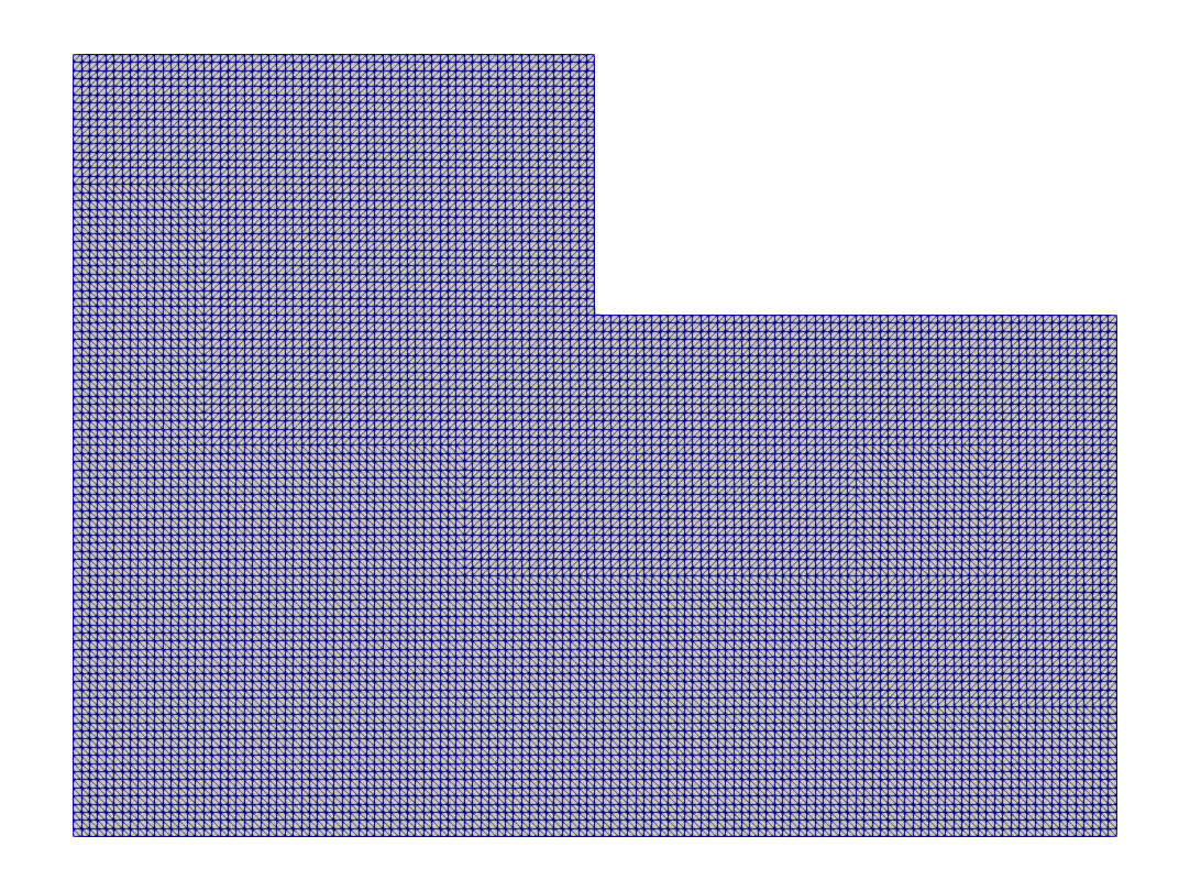
Figure 2: Basic (medium) computational grid

Figure 3: Solution $v_{\alpha}(\bm{x})$ of the diffusion–reaction problem for $\alpha=2^{-8}$

In solving this problem, the key point is the dependence of the solution on the small parameter $\alpha$. The numerical solution obtained on a very fine grid with $\alpha=2^{-8}$ is treated as the exact one. The solution $v_{\alpha}(\bm{x})$ of the auxiliary problem (12), (13) under these conditions is presented in Fig. 3, and the corresponding function $u_{\alpha}(\bm{x})$, determined according to (14), is shown in Fig. 4. The influence of the parameter $\alpha$ can be observed in Fig. 5, where the solution in the cross section $x_{1}=x_{2}$ is plotted (the red line in Fig. 5). In our model problem, a good accuracy is achieved for $\alpha\approx 2^{-7}$.

Figure 4: Solution $u_{\alpha}(\bm{x})$ at $\alpha=2^{-8}$

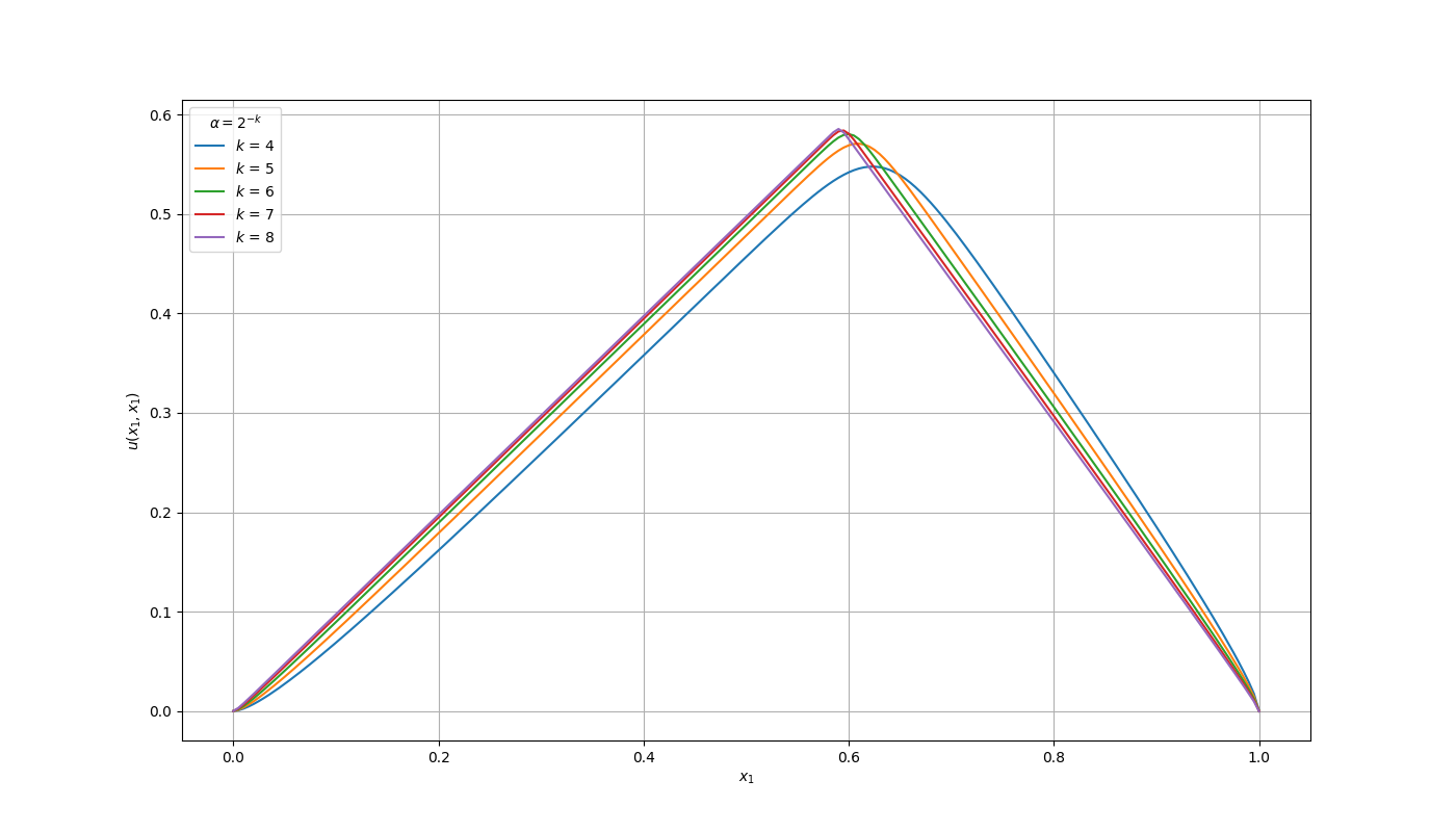
Figure 5: Solution $u_{\alpha}(\bm{x})$ in the section $x_{1}=x_{2}$ for various $\alpha$

The increase in accuracy can be achieved, first of all, by using finer grids. The solution for various $\alpha$ on the coarse grid (2,673 nodes and 5,120 triangles) is given in Fig. 6. In this case, for $\alpha=2^{-k},\ k\geq 6$, the solution is non-monotone, i.e., at some nodes of the computational grid we have $y(\bm{x})<0$. Similar data for the basic grid are presented in Fig. 7. Here, the non-monotonicity appears at $\alpha=2^{-k},\ k\geq 7$. Figure 8 demonstrates the numerical results obtained on the fine grid (41,409 nodes and 81,920 triangles). The non-monotonicity of the approximate solution occurs at $\alpha=2^{-k},\ k\geq 8$.

In the practical use of the approach (12)–(14), it seems reasonable to follow the next strategy. We solve a number of auxiliary problems (12), (13) with a step-by-step decrease of the parameter $\alpha$ as long as the maximum principle holds. The solution obtained with the smallest $\alpha$ is taken as the approximate solution of the problem (5)–(7).

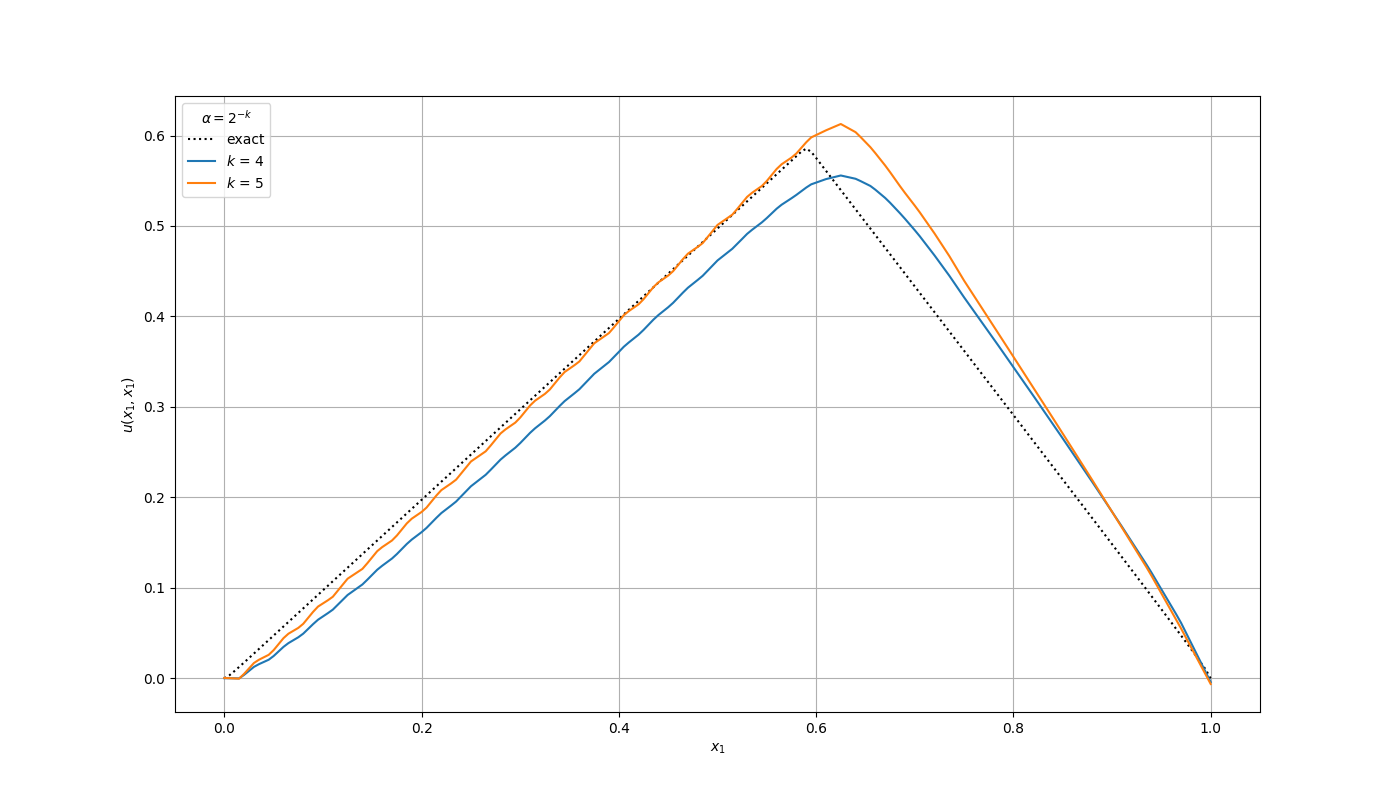
Figure 6: Solution $u_{\alpha}(\bm{x})$ in the section $x_{1}=x_{2}$ for various $\alpha$ — the coarse grid

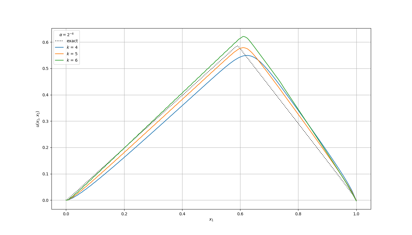
Figure 7: Solution $u_{\alpha}(\bm{x})$ in the section $x_{1}=x_{2}$ for various $\alpha$ — the basic (medium) grid

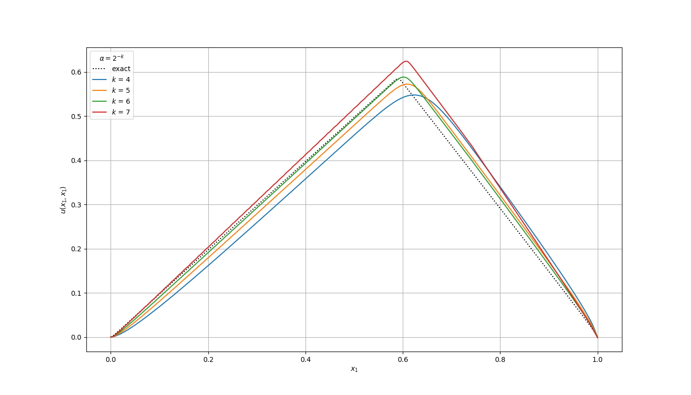
Figure 8: Solution $u_{\alpha}(\bm{x})$ in the section $x_{1}=x_{2}$ for various $\alpha$ — the fine grid

Our computational grids consist of rectangular isosceles triangles. Because of this, the non-monotonicity is due to the reaction coefficient only. To monotonize discrete solutions, it is sufficient to apply the standard procedure of the reaction coefficient lumping [37]. The effect of diagonalization of the reactive term in the finite-element approximation in predictions on different computational grids can be observed in Figures 9–11. In this case, the maximum principle holds for all $\alpha$.

The accuracy of the approximate solution decreases from some value of $\alpha$ as the parameter $\alpha$ decreases. Moreover, the value of this optimal value is close to the value that we had without the lumping procedure. Therefore, we can use the diagonalization procedure for selecting the parameter $\alpha$ using the monotonicity condition for the discrete solution of the standard finite-element approximation. In our case (see Figures 6–8), we select $\alpha=2^{-5}$ for the coarse grid, $\alpha=2^{-6}$ — for the basic grid and $\alpha=2^{-7}$ — for the fine grid.

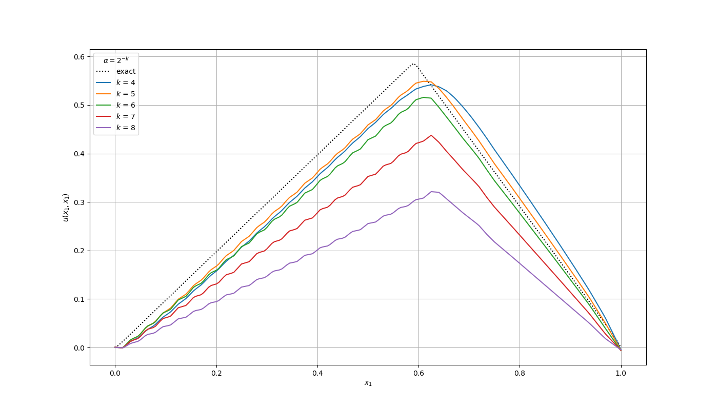
Figure 9: Reaction coefficient lumping for various $\alpha$ — the coarse grid

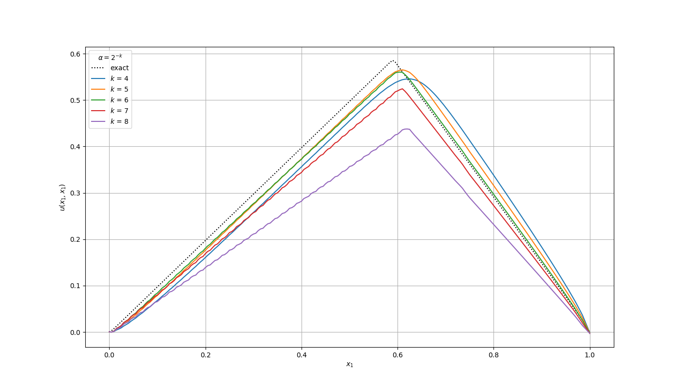
Figure 10: Reaction coefficient lumping for various $\alpha$ — the basic (medium) grid

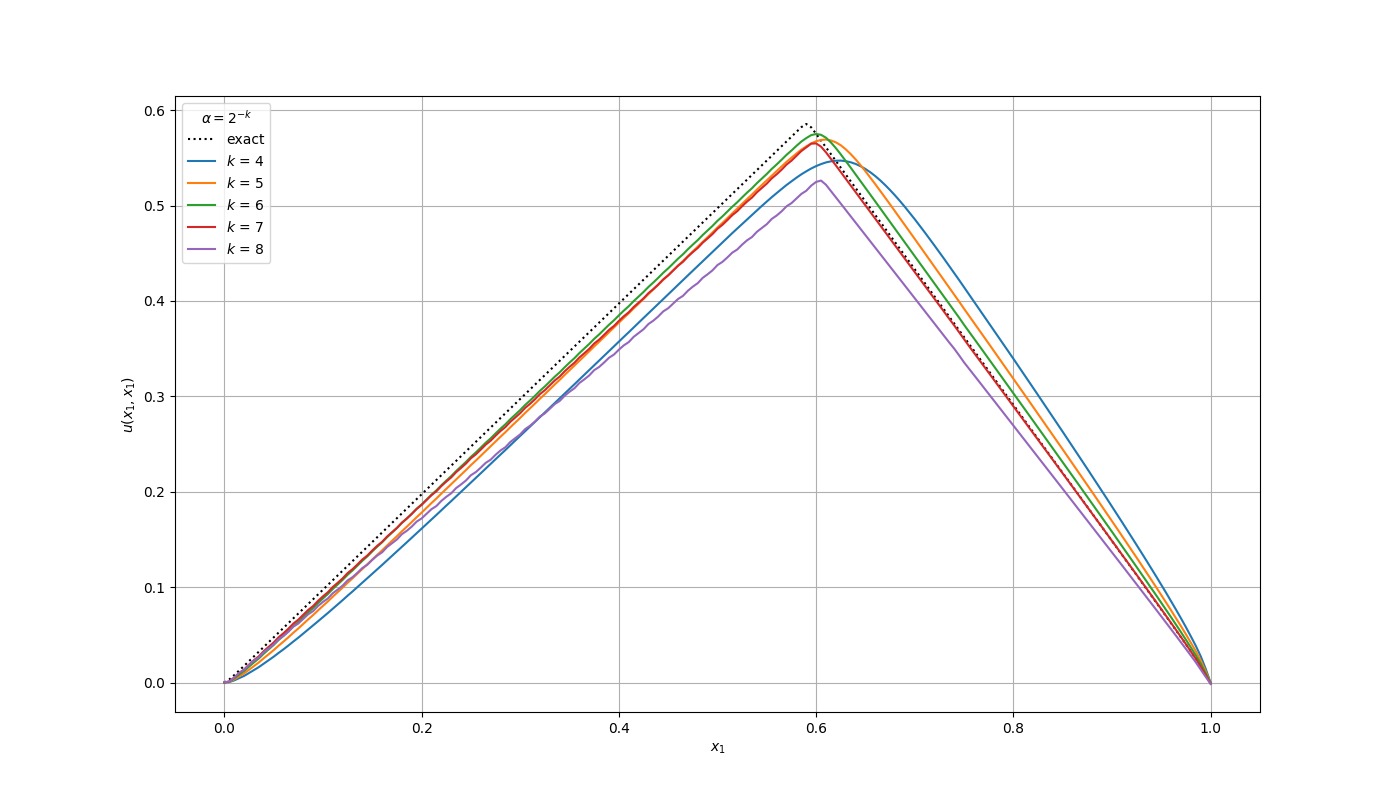
Figure 11: Reaction coefficient lumping for various $\alpha$ — the fine grid

Above, we have used linear finite elements. Below, we will present numerical results obtained on the basic grid for Lagrangian finite elements of degree $m$, i.e., for approximations $P_{m},\ m>1$. Figure 12 demonstrates the approximate solution obtained using finite elements of degree 3. A comparison with the case $m=1$ (see Fig. 7) indicates that the solution is more accurate and, in addition, it is possible to carry out calculations with a smaller value of the parameter $\alpha$. These effects become more pronounced when using finite elements of degree 5 (see Fig. 13) and degree 7 (see Fig. 14).

Thus, the computational algorithm for solving the eikonal equation (BVP (5)–(7)) can be based on the solution of the auxiliary problem (12), (13). In doing so, we employ the minimum value of the parameter $\alpha$ that provides the monotone solution on sufficiently fine computational grids using higher degree Lagrangian finite elements.

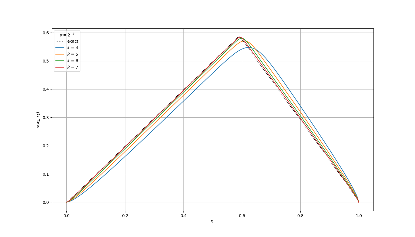
Figure 12: Solution $u_{\alpha}(\bm{x})$ in the section $x_{1}=x_{2}$ for various $\alpha$ — approximation $P_{3}$

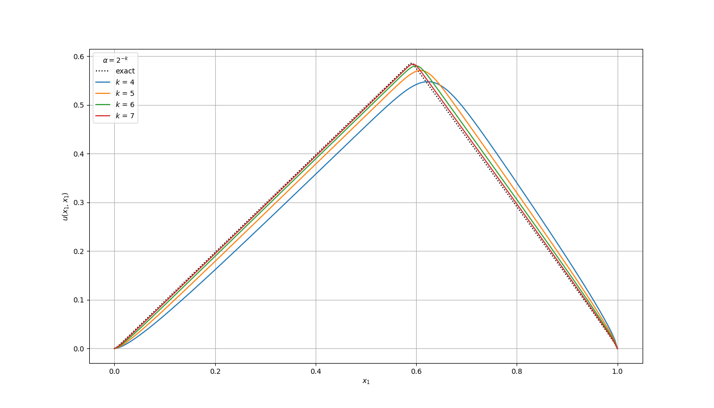
Figure 13: Solution $u_{\alpha}(\bm{x})$ in the section $x_{1}=x_{2}$ for various $\alpha$ — approximation $P_{5}$

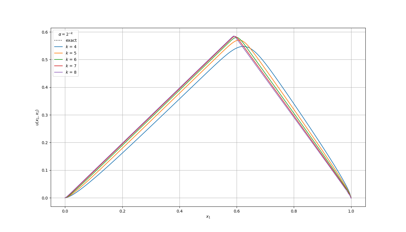
Figure 14: Solution $u_{\alpha}(\bm{x})$ in the section $x_{1}=x_{2}$ for various $\alpha$ — approximation $P_{7}$

Special attention should be paid to the problem (5)–(7) in the anisotropic case. We have considered a variant with constant coefficients, where in (6), we had

$$a_{1}^{2}=1,\quad a_{2}^{2}=4.$$

The convergence of the approximate solution with decreasing $\alpha$ is given in Fig. 15. Calculations have been performed on the basic grid using finite-element approximation with $P_{7}$. The numerical solution of the problem (5)–(7) for $\alpha=2^{-8}$ is shown in Fig. 16. Similar data obtained for a more pronounced anisotropy:

$$a_{1}^{2}=1,\quad a_{2}^{2}=10,$$

are depicted in Fig. 17, 18.

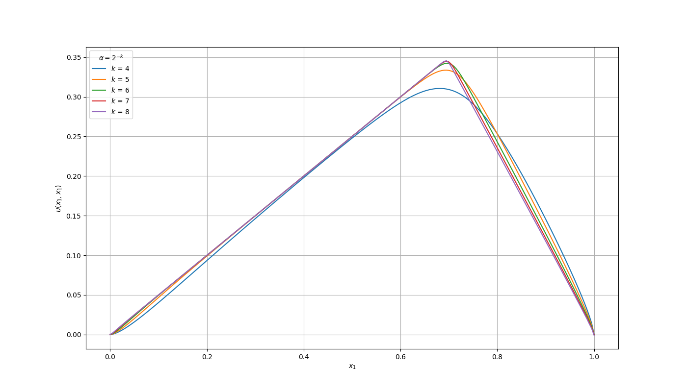
Figure 15: Solution $u_{\alpha}(\bm{x})$ in the section $x_{1}=x_{2}$ for various $\alpha$ — $a_{1}^{2}=1,\ a_{2}^{2}=4$

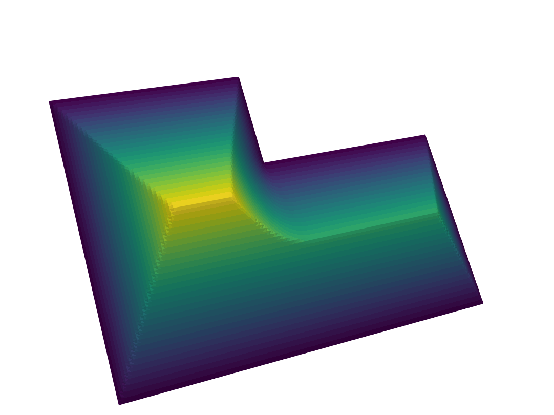
Figure 16: Approximate solution $u_{\alpha}(\bm{x})$ for $\alpha=2^{-8}$ at $a_{1}^{2}=1,\ a_{2}^{2}=4$

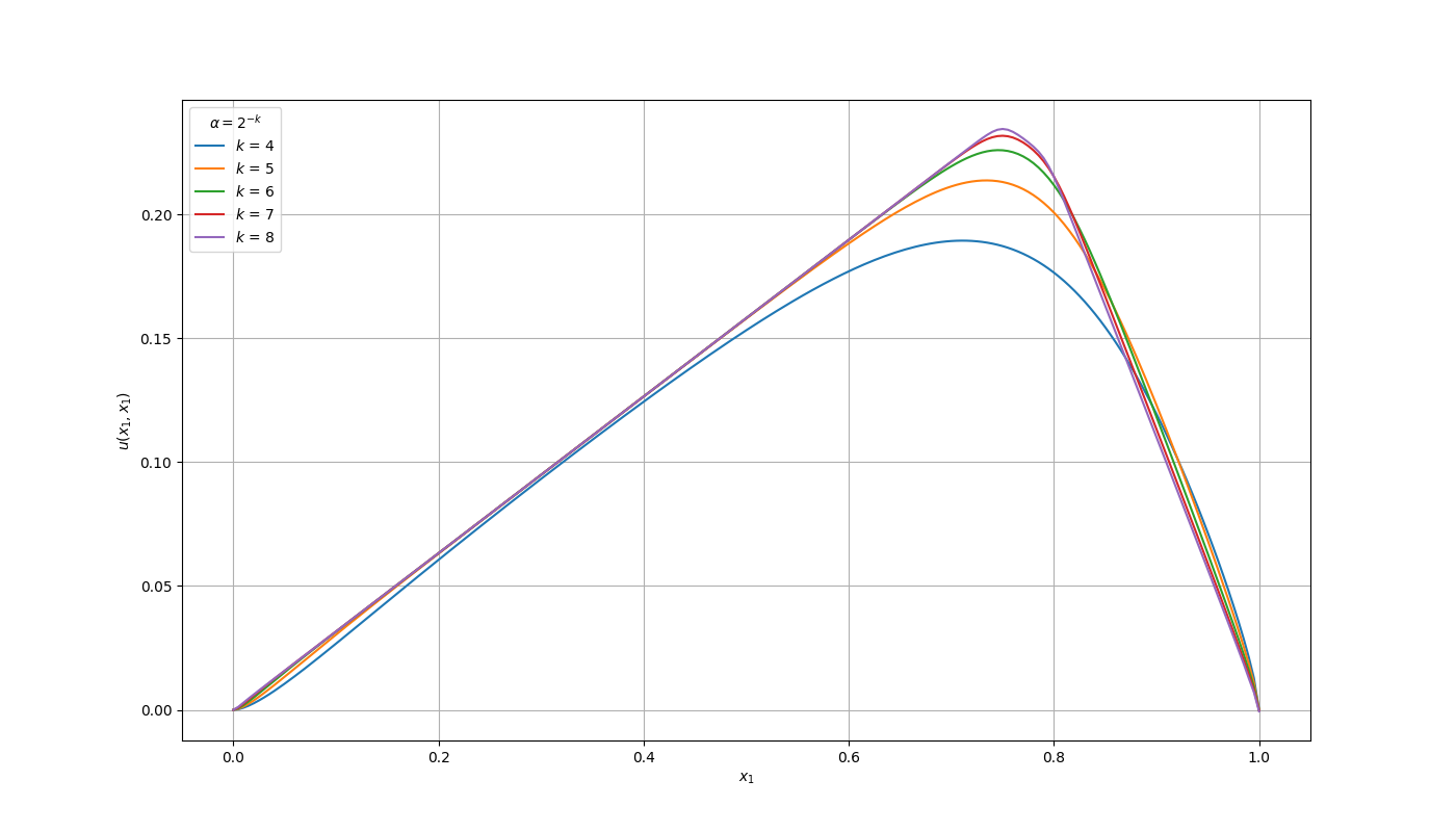
Figure 17: Solution $u_{\alpha}(\bm{x})$ in the section $x_{1}=x_{2}$ for various $\alpha$ — $a_{1}^{2}=1,\ a_{2}^{2}=10$

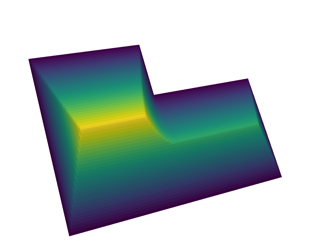
Figure 18: Approximate solution $u_{\alpha}(\bm{x})$ for $\alpha=2^{-8}$ at $a_{1}^{2}=1,\ a_{2}^{2}=10$

5 Conclusions

1. A Dirichlet problem is considered for the multidimensional eikonal equation in a bounded domain with an anisotropic medium. The main peculiarities of such problems results from the fact that the eikonal equation is nonlinear.

2. An approximate solution is constructed using a transformation of the original nonlinear boundary value problem to a linear boundary value problem for the diffusion–reaction equation for an auxiliary function. The transformed equation belongs to the class of singularly perturbed problems, i.e., there is a small parameter at higher derivatives.

3. Computational algorithms are constructed using standard finite-element approximations on triangular (2D problems) or tetrahedral (3D problems) grids. Monotonization of a discrete solution is achieved not only by using finer grids, but also via a correction of approximations for the reaction coefficient using the lumping procedure. The use of finite elements of high degree is studied, too.

4. Numerical experiments have been performed for 2D problems in order to demonstrate the robustness of the approach proposed in the work for solving boundary value problems for the eikonal equation in an anisotropic medium. In particular, a good accuracy is observed when using sufficiently fine grids and Lagrangian finite elements of higher degree.

References

- [1] M. Born, E. Wolf, Principles of Optics: Electromagnetic Theory of Propagation, Interference and Diffraction of Light, Cambridge university press, 2005.
- [2] Y. A. Kravtsov, Y. I. Orlov, Geometrical Optics of Inhomogeneous Media, Springer, 1990.
- [3] J. A. Sethian, Level Set Methods and Fast Marching Methods: Evolving Interfaces in Computational Geometry, Fluid Mechanics, Computer Vision, and Materials Science, Vol. 3, Cambridge university press, 1999.
- [4] A. Gilles, K. Pierre, Mathematical Problems in Image Processing: Partial Differential Equations and the Calculus of Variations, Springer, 2006.
- [5] S. N. Kružkov, Generalized solutions of the Hamilton-Jacobi equations of eikonal type. I. Formulation of the problems; existence, uniqueness and stability theorems; some properties of the solutions, Sbornik: Mathematics 27 (3) (1975) 406–446.
- [6] P.-L. Lions, Generalized Solutions of Hamilton-Jacobi Equations, Pitman, 1982.
- [7] J. Tsitsiklis, Fast marching methods, IEEE Transactions on Automatic Control 40 (1995) 1528–1538.
- [8] J. A. Sethian, Fast marching methods, SIAM Review 41 (2) (1999) 199–235.
- [9] Y.-H. R. Tsai, L.-T. Cheng, S. Osher, H.-K. Zhao, Fast sweeping algorithms for a class of Hamilton–Jacobi equations, SIAM Journal on Numerical Analysis 41 (2) (2003) 673–694.
- [10] H. Zhao, Fast sweeping method for eikonal equations, Mathematics of Computation (74) (2005) 603–627.
- [11] W.-K. Jeong, R. T. Whitaker, A fast iterative method for eikonal equations, SIAM Journal on Scientific Computing 30 (5) (2008) 2512–2534.
- [12] Z. Fu, W.-K. Jeong, Y. Pan, R. M. Kirby, R. T. Whitaker, A fast iterative method for solving the eikonal equation on triangulated surfaces, SIAM Journal on Scientific Computing 33 (5) (2011) 2468–2488.
- [13] Z. Fu, R. M. Kirby, R. T. Whitaker, A fast iterative method for solving the eikonal equation on tetrahedral domains, SIAM Journal on Scientific Computing 35 (5) (2013) C473–C494.
- [14] J. V. Gómez, D. Alvarez, S. Garrido, L. Moreno, Fast methods for eikonal equations: an experimental survey, arXiv preprint arXiv:1506.03771.
- [15] A. G. Belyaev, P.-A. Fayolle, On variational and PDE-based distance function approximations, in: Computer Graphics Forum, Vol. 34, Wiley Online Library, 2015, pp. 104–118.
- [16] C. Li, C. Xu, C. Gui, M. D. Fox, Level set evolution without re-initialization: a new variational formulation, in: Computer Vision and Pattern Recognition, 2005. CVPR 2005. IEEE Computer Society Conference on, Vol. 1, IEEE, 2005, pp. 430–436.
- [17] E. Fares, W. Schröder, A differential equation for approximate wall distance, International Journal for Numerical Methods in Fluids 39 (8) (2002) 743–762.
- [18] T. Bhattacharya, E. DiBenedetto, J. Manfredi, Limits as of and related extremal problems, Rendiconti del Seminario Matematico Universit‘a e Polytecnico di Torino 47 (1989) 15–68.
- [19] B. Kawohl, On a family of torsional creep problems, J. Reine Angew. Math 410 (1) (1990) 1–22.
- [20] K. S. Gurumoorthy, A. Rangarajan, A Schrödinger equation for the fast computation of approximate Euclidean distance functions, in: International Conference on Scale Space and Variational Methods in Computer Vision, Springer, 2009, pp. 100–111.
- [21] M. Sethi, A. Rangarajan, K. Gurumoorthy, The Schrödinger distance transform (SDT) for point-sets and curves, in: Computer Vision and Pattern Recognition (CVPR), 2012, IEEE, 2012, pp. 198–205.
- [22] K. Crane, C. Weischedel, M. Wardetzky, Geodesics in heat: A new approach to computing distance based on heat flow, ACM Transactions on Graphics (TOG) 32 (5) (2013) 152.
- [23] H. Roos, M. Stynes, L. Tobiska, Robust Numerical Methods for Singularly Perturbed Differential Equations: Convection-Diffusion-Reaction and Flow Problems, Vol. 24, Springer Science & Business Media, 2008.
- [24] J. J. H. Miller, E. O’Riordan, G. I. Shishkin, Fitted Numerical Methods for Singular Perturbation Problems: Error Estimates in the Maximum Norm for Linear Problems in One and Two Dimensions, World Scientific, 2012.
- [25] S. C. Brenner, L. R. Scott, The Mathematical Theory of Finite Element Methods, Springer, New York, 2008.
- [26] M. G. Larson, F. Bengzon, The Finite Element Method: Theory, Implementation, and Applications, Springe, 2013.
- [27] A. V. Bitzadze, Some Classes of Partial Differential Equations, Nauka, 1981, in Russian.
- [28] L. C. Evans, Partial Differential Equations, AMS, 2010.
- [29] M. H. Holmes, Introduction to Perturbation Methods, Springer, 2012.
- [30] F. Verhulst, Methods and Applications of Singular Perturbations: Boundary Layers and Multiple Timescale Dynamics, Springe, 2005.
- [31] M. H. Protter, H. F. Weinberger, Maximum Principles in Differential Equations, Springer, 2012.
- [32] D. Gilbarg, N. S. Trudinger, Elliptic Partial Differential Equations of Second Order, springer, 2015.
- [33] F. W. Letniowski, Three-dimensional Delaunay triangulations for finite element approximations to a second-order diffusion operator, SIAM Journal on Scientific and Statistical Computing 13 (3) (1992) 765–770.
- [34] W. Huang, Discrete maximum principle and a delaunay-type mesh condition for linear finite element approximations of two-dimensional anisotropic diffusion problems, Numerical Mathematics: Theory, Methods and Applications 4 (3) (2011) 319–334.
- [35] P.-A. Ciarlet, P. G.and Raviart, Maximum principle and uniform convergence for the finite element method, Computer Methods in Applied Mechanics and Engineering 2 (1) (1973) 17–31.
- [36] J. H. Brandts, S. Korotov, M. Křížek, The discrete maximum principle for linear simplicial finite element approximations of a reaction–diffusion problem, Linear Algebra and its Applications 429 (10) (2008) 2344–2357.
- [37] V. Thomée, Galerkin Finite Element Methods for Parabolic Problems, Springer Verlag, Berlin, 2006.
- [38] Q. Cai, S. Kollmannsberger, E. Sala-Lardies, A. Huerta, E. Rank, On the natural stabilization of convection dominated problems using high order Bubnov–Galerkin finite elements, Computers & Mathematics with Applications 66 (12) (2014) 2545–2558.