Reducing and Analyzing the PHAT Survey with the Cloud

Abstract

We discuss the technical challenges we faced and the techniques we used to overcome them when reducing the PHAT photometric data set on the Amazon Elastic Compute Cloud (EC2). We first describe the architecture of our photometry pipeline, which we found particularly efficient for reducing the data in multiple ways for different purposes. We then describe the features of EC2 that make this architecture both efficient to use and challenging to implement. We describe the techniques we adopted to process our data, and suggest ways these techniques may be improved for those interested in trying such reductions in the future. Finally, we summarize the output photometry data products, which are now hosted publicly in two places in two formats. They are in simple fits tables in the high-level science products on MAST, and on a queryable database available through the NOAO Data Lab.

1. Introduction

Large catalogs are an important component of observational astronomy. Entire research programs that only analyze public catalogs are becoming common (e.g., Yang et al., 2007; Ivezić et al., 2007; Shen et al., 2011; Kleinman et al., 2013; Tempel et al., 2014; Salim et al., 2016; Tian et al., 2017; Bobylev & Bajkova, 2017). The production of these catalogs, and the interfaces by which they are served to the public will be of significant concern in the coming decade, especially for projects like LSST and missions like WFIRST, which will be cataloging large numbers of measurements of billions of sources (Ivezic et al., 2008; Spergel et al., 2013; Williams, 2015). One option for handling the computational challenges surrounding producing and analyzing these catalogs is using commercial cloud compute services such as Amazon’s Elastic Computing Cloud (EC2).

There are an increasing number of computer use cases in astronomy research that require a large amount of computing power for small periods of time. For such projects, it is not efficient to purchase large compute clusters or a large number of computers. Furthermore, many institutions do not allow users to have root access to their machines. However, commercial services that provide computing at an hourly rate allow researchers to obtain access to a nearly unlimited amount of computing power. If the amount of time they need is relatively short, the cost can be much cheaper than purchasing machines. Furthermore, they can have complete control of the operating system as root users, simplifying software installation and allowing streamlined memory use.

With a cloud-based system, one can hire as many processors as necessary only for the time needed to do the work. Thus, if a processing job that takes a week on a single machine can be distributed among hundreds of machines, it can be done in a few minutes for a few dollars, without the need to purchase a large compute cluster.

This capability can be quite cost-effective for astronomers, as observational data sets can be quite large, but many programs may only need to reduce one very large data set each year. This reduction may require a large amount of computing, but once it is done for the year, the need for a large amount of computing power is gone, making purchasing computers highly inefficient in such cases.

Another difficulty surrounding working with large data sets is sharing the output catalogs with the community. Once the photometric measurements are complete, they should be served in a format that is useful for the community. The Sloan Digital Sky Survey (SDSS York et al., 2000; Aihara et al., 2011; Abolfathi et al., 2017) set the standard for one solution to this problem, which is to serve the catalogs using the SkyServer (Szalay et al., 2001) web-based database interface.

SDSS SkyServer serves a Microsoft SQL Server database with a flexible web-based search form that is now typical for many catalog services, such as Vizier (Ochsenbein et al., 2000) and the SAO/NASA Astrophysics Data System (ADS Kurtz et al., 2000). For SDSS catalog access, its most powerful features are the ability to issue direct SQL queries to the server both in real time and in batch mode, and to store results in personal database tables. This approach allows users to formulate scientific questions as queries with all the necessary complexity, creating subsamples of the catalog to be downloaded for further analysis.

For future large surveys, such as the 10-year survey to be undertaken by the Large Synoptic Survey Telescope (LSST LSST Science Collaboration et al., 2009), the data volume requires new database technology development, and even catalog subsamples will often be too large to download efficiently. LSST will extend the approach used by SDSS, developing a new database architecture to be able to scale to LSST’s data requirements (Wang et al., 2011), and allowing complex analysis to run on servers close to the catalog and image data itself (through the LSST Science Platform), thus avoiding massive downloads of data. Indeed, a number of projects have begun implementing such science platforms for use on existing large datasets, including CANFAR (Gaudet et al., 2010), SciServer (http://sciserver.org), and the NOAO Data Lab (Fitzpatrick et al., 2014). With large volumes of data becoming common for many smaller programs, the need for such platforms to provide efficient data interfaces is growing, in particular because small programs rarely have the resources to develop such interfaces for themselves.

One of the first large survey programs to be reduced using commercial cloud resources was the PHAT survey (Williams et al., 2014, hereafter, W14). Herein we will describe the challenges faced and techniques used in reducing the PHAT data using a cloud service. We used Amazon Web Services (AWS), so we discuss AWS applications in detail, but but other cloud service providers (such as Google Cloud Services, Microsoft Azure, Oracle Cloud etc.) also offer similar functionality. Section 2 gives an overview to the technical aspects of EC2. Section 3 describes the PHAT pipeline architecture, which works well on such cloud computing platforms. Section 4 discusses the importance of monitoring systems for keeping track of pipeline jobs and handling problems. Section 5 describes our photometry database schema, and section 6 provides an example of how to use the database. Finally, we conclude with a summary of the paper in Section 7 and a brief discussion of newer cloud computing features in the Appendix.

2. Amazon Cloud Computing and Storage

Amazon offers on-demand computing resources primarily through the AWS Elastic Compute Cloud (EC2). As with other cloud computing services, this service has a virtually unlimited amount of compute power available at any given time, but one must access and use the resource carefully to make it cost-effective. In this section, we describe the various aspects of EC2, and how they work together to provide a powerful computing resource for the community.

2.1. Instances

Computer clouds are large numbers of individual computing cores. Amazon calls each of these cores “instances,” which are compute nodes that are assigned to user accounts upon request. Launching these instances requires an Amazon Web Services account, as well as an Amazon Machine Image (AMI). Users are then charged for the amount of time each requested instance is running.

Instances have multiple pricing options, which range over an order of magnitude. The most expensive is ”on-demand.” If an instance with this pricing option is requested it instantly starts booting up, and it will stay operational until the user explicitly terminates it. These instances have very high reliability, but are much more expensive than simply buying a computer, if they are going to be up for more than a few months per year. However, they may still be of great use to those who either wish to have a reliable instance in the cloud for quick and free access to storage, high bandwidth communication to other instances, or rapid and reliable availability.

The next option is ”reserved.” These instances are rented for periods of years as a contract. Once they are reserved, they stay up for the full year, whether they are in use or not. This is the best option for instances you know you will need to be up for many months, since they are typically cheaper than on-demand by a factor of a few if both are being constantly used for months at a time.

Finally, there is the cheapest option, which is called ”spot.” The price of these instances is dynamic, and changes by the minute. Typically, the price is less than 20% of the on-demand price. One specifies a maximum price for these instances, and if the price goes above that maximum, the instance is automatically terminated without warning. When the price is below the bid, the user pays the price, not what they bid, so that if the price is one cent per hour and the bid is one dollar per hour, the user will pay one cent, but if the price is one dollar, they will pay one dollar. If it goes to one dollar and one cent, then the instance vanishes, along with all of the data on it. This requires some care and thought with the bidding, as the instance price can fluctuate significantly, as shown in the example in Figure 1.

2.2. Costs

There are several factors to consider when deciding between using cloud based services or purchasing hardware. One of the most important of these for many users is the cost. One must consider whether it will cost more to develop and use an analysis pipeline on a cloud server or on a private compute cluster. A few of issues we found important for estimating the cost different were the duration of the project, the computing demands profile, and the likelihood of other projects that may also be able to run on the cloud in the future.

Project duration is important to consider when estimating the costs of the cloud vs. purchasing hardware. Both short and long projects may suffer from purchasing hardware. Short projects may be delayed waiting for hardware to be ordered, delivered, set up, and managed. Long projects may develop hardware that runs past its service contract, fails, or becomes obsolete. In general, projects of about 3 years tend to benefit from hardware purchase, since that uses the full typical service contract window, and if getting going takes a couple of months, that is only a small fraction of the project time.

The computing demands profile is also important to consider. Even if the project is an appropriate duration for a typical hardware contract, the project may only need a large amount of processing power for a few weeks per year. In this case, 100 instances on a cloud system would only cost $\sim$$5k per year, and a compute cluster may cost closer to $\sim$$100k for the hardware alone.

It is also important to consider if the development costs to run on the cloud may pay off with future projects. Perhaps the project has a duration and demand profile that put purchasing hardware and using cloud resources at similar cost. In this case, perhaps developing the ability to use the cloud is worthwhile if it will allow future projects to use the ability. For example, while the cost to develop the PHAT pipeline on EC2 was comparable to the cost to purchase our own cluster, we have been able to use the infrastructure we developed for many other HST projects. On the other hand, if we had purchased hardware, it would be well past its expected lifetime by now.

Ideally it would be helpful to know how much it costs to develop a pipeline server that can be used in the way we outline in this paper. However, because our pipeline was developed over the course of over a year, by several scientists and software engineers, and overcame many issues that no longer exist, it is difficult to estimate how much it would cost a team to do this today. Still, it is likely to cost about 1 full-time employee for one year with significant experience with designing database systems and working with application programming interfaces (APIs) to build the master instance image, the job handler, and the monitoring system. This estimate is likely an upper limit given the increased availability of tools to make this kind of computing easier to implement (see Appendix). For us, this work was split as partial support for several people. With overheads, this effort amounts to about $\sim$$200k, which does not include the cost of the cloud computing itself (typically $\sim$$0.05 per CPU hour for spot instances).

Developing a pipeline to run on purchased hardware has a cost as well. In this case, one still needs to develop a job handling system and a way to monitor the jobs. However, this kind of set up is much simplified because of the lower security concerns, shared storage, and scheduler software that come with most compute clusters. In addition, one must pay for the purchase, power, storage, and administration of the hardware. Typical hardware for a $\sim$20 node compute cluster would be $\sim$$100k; adding in typical service contracts, storage, software licenses, and other expenses, brings this to $\;\buildrel>\over{\sim}\;$$200k for 3 years of use. Using such a cluster efficiently still requires some kind of pipeline architecture that, while simpler than developing a cloud-based pipeline, has its own development costs associated with it. All of these costs should be compared to the number of CPU hours one intends to use and the need for longer term applications to see how it compares to a one-time $\sim$$200k development cost plus $\sim$$0.05 per CPU hour, that one may expect to pay to do the project with cloud services.

2.3. Machine Images

Cloud computing systems rely on the user to supply a computing operating system and environment that can be easily replicated on as many machines as are requested. Most commercial cloud computing services will likely use something like a full snapshot from a working compute node to allow such replication. Such snapshots provide users with the flexibility to tailor their operating system to their needs. They contain a complete copy of the software and data needed to start an individual worker machine, including the operating system. In case of AWS, these snapshot files are called Amazon Machine Images (AMIs).

Amazon has several options for starter AMIs, which contain enough capabilities to allow an instance to boot and allow a user to log in. Then, the user can customize the AMI by installing the software they require for their data analysis. Once all of that software is installed and working properly, the user can save the AMI under their own account. Then, the user can replicate as many copies of that AMI as often as they wish. Thus, once the user has an AMI capable of running their data analysis software, they can generate 1, 10, or thousands of instances with those capabilities.

2.4. Storage

One challenging aspect to analyzing data on the cloud is the lack of shared disk space between machines. In most cloud systems, the individual machines only see their own local storage, not that of other machines in the cloud. In our AWS example, instances on EC2 act as stand-alone computers. Their storage is local, and disappears when the user turns off the instance. However, Amazon has a very large separate storage service, called Simple Cloud Storage Service‎ (S3), which is always available to any machine connected to the internet. Any data pushed from the instance to S3 will be safe. Thus, a significant challenge in leveraging many instances is making sure that they each have the correct version of any file that is being analyzed.

We show the storage design in Figure 2. For example, if a process updates the cosmic ray masking of an image, and another process runs searches for celestial light sources on the image, then the instance that runs the former must push its updated file to S3, and the instance that runs the latter must pull that updated version from S3. Keeping files synchronized across the worker nodes proved to be very challenging and required a significant amount of custom software when we built our pipeline. However, the advantage of all of this effort is that all of the most up-to-date products are always on S3, which simplifies recovery from losing instances and makes all products instantly available anywhere in the world.

2.5. Security

To use EC2, or likely any commercial cloud service, one must have an account which gets charged for the resources used. On AWS, this account comes with keys that allow one to start instances and move data. The charge for the resources is then applied to the account associated with the keys. For large amounts of data reduction, it is critical to be able to quickly start, track, and terminate many instances. For us, this meant automating spot requests for new instances and the ability to for those instances pull data from and push data to S3. Thus our instances have our keys, and if they were successfully hacked, the hackers could take our keys and run a huge amount of computing, billing it to our accounts without us ever finding them. Therefore, security is extremely important.

A surprisingly large amount of the development to move to the commercial cloud was automating all of the security calls in a safe way. Two key parts to this were making sure there was only one open port on our nodes, and only allowing information with very specific formats through those ports. Limiting the communication possible with an instance is straight-forward in EC2, but making it work with an automated pipeline architecture is a challenge, which we will describe further in Section 3.

3. Pipeline Architecture

A software pipeline is typically understood to be a series of scripts run on a set of input files that produces useful products from those files. In the case of PHAT, the pipeline started from the HST-provided calibrated images, and from those images, produced clean mosaic images, in all bands, color images, catalogs of resolved stellar photometry, artificial star tests, and many diagnostic and scientific plots from each step in the process.

To keep track of all of these tasks while they were being performed on thousands of images, we adopted a master-worker pipeline architecture, which we show with a schematic drawing in Figure 3. This architecture requires one machine that keeps track of all the jobs being done while any number of other machines actually do the jobs. The master machine needs to be a server that is able to communicate with many other machines simultaneously. It does not require any analysis software, but instead requires sophisticated communication and security software. The worker machines can all be identical as long as they all have the appropriate software to perform the analysis jobs and to report back to the master machine.

To run a master-worker pipeline requires two AMIs: one for the master, and one for the workers. Our master AMI is a specially configured (networking, security, backup, SVN-repository) Linux-box (AWS Linux or Ubuntu) functioning as a webserver (Apache$+$Passenger or Unicorn$+$Nginx) running a highly customized web-application (Ruby on Rails) interfaced with a traditional database (mySQL) that is queried by scripts running on worker instances via HTTP requests which are generated and the corresponding responses parsed using an utility suite (Java). We ran this AMI on an on-demand instance, so that we could be sure the server would stay up. More efficient may be to host the server on a reserved instance if the user knows they’ll be using their pipeline semi-regularly for a long time, whereas a more economic solution is running the server on a spot instance with an unusually high bid and a reliable, frequent backup system if the pipeline infrastructure will only be used intermittently.

For reducing the PHAT software, our worker AMI needed many custom additions, including PyRAF, IDL, DOLPHOT, and all of our pipeline communication software, which in our case was Perl scripts that called our suite of Java tools for querying the server. These tools had all of the necessary capabilities back in 2009 when we started the project. For any future pipeline builds, we would recommend using python since it has all of the necessary capabilities now and is better supported by the community. Also, keeping all of the steps within one language will make finding and fixing bugs much more straight-forward.

One advantage of the master-worker architecture for cloud computing is that one can request as many worker nodes as one needs to get the work done, and then scale back when the work completes. Furthermore, if the server is designed to recover from failures efficiently, all of the worker nodes can be on spot instances, reducing the compute cost by up to an order of magnitude. We set up our pipeline for reducing the PHAT data using spot instance workers.

Our pipeline used an event based routine to keep track of jobs. Each job consists of an executable script called a task, the conditions under which the task is to be run, and any options that need to be passed to that task. Before running data through the pipeline, the user registers all of the executable scripts that are part of the pipeline. This enters the names and options for those scripts into a database that records how events trigger the tasks. A task may produce events that trigger many other tasks. These can then produce their own events that trigger even more tasks, and so on, until the pipeline is complete. Each event is stored as an entry in the database, and it contains all of the information needed to run the task that it triggers. Thus, if a task fails, it can easily be restarted simply by pointing the pipeline to the event that triggered that task. In this way, recovering from failed tasks is simple and efficient, as one never needs to rerun successfully completed tasks.

This architecture is especially important for EC2, since a spot instance worker can disappear at any time, causing all of its running tasks to fail. In addition, tasks may fail due to some other problem, such as a data set that has different properties that the pipeline task expects or a failed data transfer from S3. Virtually all failures are efficient to fix within our architecture, which also allows us to debug a task and then retry it without restarting the pipeline run from the beginning.

Furthermore, this architecture makes it possible to create an extremely secure pipeline by pushing all communication through a single instance. The server is the largest security risk, as it must be allowed to receive data; however, it can be configured to only allow incoming data of a format known only to the worker nodes, and the worker nodes can be configured to only accept incoming data from the server’s ip address. Since all of the workers are copies of one another, this security can be part of the worker AMI. This technique makes the user free to carefully set up and monitor the security of only one instance to keep all of the accounts secure.

4. Monitoring

Because the pipeline performs many tasks on a large number of data sets, it is critical to have a simple way to monitor the events and jobs to easily spot, investigate, or restart failures. Because our pipeline architecture works by keeping a database of tasks and events, we are able to simply display these tasks and events, along with their pipeline state and the instance on which they were executed, in a tree diagram. This tree is populated directly from the database, and it simply shows all of the work that has been and is currently being done within the pipeline, allowing an easy scan by eye or with a find tool, to look for any problems. When a problem is spotted, it is then easy to find the data associated with the problem through the information associated with the event. We show an example from our system in Figure 4, where we included a failed job to highlight how this system makes it easy to track and troubleshoot such problems.

5. Photometry Database

Once the computing is complete, a huge amount of reduced data are available. These reduced data are in the form of tables that have rows of measurements. Each measurement typically will have many values associated with it, such as the time the observation was taken, the filter, the count rate measured, the background level, and any quality metrics about the pixels measured. Putting all of this data into an efficient and intuitive database is the next challenge in the process of managing such large observing programs.

For PHAT, our original data release simply supplied the images and catalogs in FITS format. While these tables and images contain reliable measurements and all of the necessary meta-data for any user to find an measurement available within the data, they are numerous, large, and complex, forcing any user to learn quite a bit about data structures in order to write code to find what they are looking for. This method for data distribution therefore does not lend itself to simple use for users interested in just a small portion of the data, such as a single object of interest.

The NOAO Data Lab (Fitzpatrick et al., 2016) became publicly available in June 2017. The goal of the Data Lab is to enable efficient exploration and analysis of large datasets, including catalogs. Among its features are a database for catalog data, accessible both through a Table Access Protocol (TAP) service and through direct PostgreSQL queries, web-based and programmatic catalog query interfaces, remote storage space for personal database tables and files, a JupyterHub-based notebook analysis environment, and a Simple Image Access (SIA) service.

We had a few reasons for hosting the PHAT catalog data in the NOAO Data Lab. First, it is being developed as a site for long-term hosting of major surveys such as the Dark Energy Survey, the Legacy Survey (the DESI targeting survey), and others, and thus ensures that the PHAT catalog will have a long shelf life. Second, the Data Lab’s existing tools and planned improvements (such as machine learning tools), will add significant analysis capability for users of the PHAT catalog now and in the future. Finally, while the current analysis model is based on notebooks running in JupyterHub, in the future Data Lab will allow fully scripted workflows running in Containers on its hardware, thus allowing for efficient automated analysis of PHAT and other datasets.

The Data Lab has some limitations on the resources provided to users, but in many cases these are soft and can be increased on a per-user basis as needed. For synchronous database queries, the standard time limit is 600 s, while for asynchronous queries, it is 12 hours. These limits should accommodate the vast majority of PHAT catalog use cases. For storage, the per-user limit is 1 TB for VOSpace virtual storage, while for myDB it is 100 GB, both of which can accommodate a significant fraction of the full PHAT catalog. For analysis in a Jupyter notebook, limits are imposed by the shared memory of the host server, which for practical purposes can accommodate  10 GB per user, or $\sim$25% of the full PHAT object catalog.

For PHAT, we ingested the combined photometric measurements for all objects in all bands and the measurements from the individual exposures, along with their meta-data, into tables in the Data Lab database. These tables allow fast access to the PHAT photometric data, and allow users to to produce sparse lightcurves and potentially look for proper motions.

Although there are not many epochs in the PHAT photometry, the data do contain a large amount of variability data. The observations were performed in 3 hour visits over four years. Each visit contained several individual exposures, allowing searches for variability on 3-hour timescales survey-wide. Furthermore, because the survey was tiled with the WFC3/IR camera, the WFC3/UVIS and ACS/WFC channels contain overlapping measurements for multiple visits over portions of the survey. This overlap allows comparisons across multiple visits, which can be separated by hours up to years, making it sensitive to variability on these timescales over portions of the survey. The available timescales change drastically with position, but in principle these overlaps can be used to probe longer timescales of variability. Finally, because the photometry for each visit was performed separately, there are separate measurements of the position of the sources in overlapping visits. These positions can, in principle, be compared to look for proper motions. The original data release, which is simple catalog files, makes such studies possible, but difficult.

To provide the necessary search capabilities to tap into the variability and proper motions information in the PHAT data, we have developed a schema for the database that allows each source to have a global identifier, combined measurement for each visit in each band that covered the sources in that visit, as well as individual measurements from each individual exposure taken during that visit. Along with the observation time, each measurement also contains all of the data quality information returned by DOLPHOT.

The photometry is organized into two main tables within a database called phat_v2; see Figure 5 for the table schema. The table phot_mod ($\sim$118 million rows) contains a unique object ID (objid) as the primary key, a unique random integer (random_id to allow for selection of random samples from the table, the averaged positions, photometry, and data quality flags for all of the objects, and spatial indices computed on the 9th order Hierarchical Triangular Mesh (HTM) and HEALPix (both NSIDE=256 RING and NSIDE=4096 NEST) systems. Many of the columns have database indices computed to allow for fast constraints on values in those columns. The data is clustered on the RA and Dec and spatially indexed with Q3C (Koposov & Bartunov, 2006) to allow for fast cone searches and spatial table joins.

The table phot_meas contains the photometry from the individual epochs, with one row per measurement ($\sim$7.5 billion rows). It contains the same unique object IDs as the phot_mod table, the times of the measurements expressed as modified Julian dates (MJD), the measured photometry and photometric flags, and metadata such as the filter used in the measurement, the exposure time, and the filename of the image from which the measurement derived. There are database indices for the MJD, RA, DEC, MAGVEGA, FILTER, BRICK, and OBJID columns, as well as a Q3C spatial index.

For completeness, the database also contains tables named phot_v2, which contain the table data in the same form as in the FITS files produced by the PHAT pipeline.

6. Data Lab Services

As mentioned above, the NOAO Data Lab provides a number of data access and analysis services for the PHAT dataset. These include:

1. Anonymous and authenticated access to Data Lab services. Anonymous users can query the database and run temporary Jupyter notebooks on the public notebook server, but cannot store results in personal database storage (myDB), access the virtual storage system (VOSpace), or save Jupyter notebooks permanently. By creating and logging into an account, authenticated users get access to a dedicated Jupyter notebook server with permanently stored notebooks, and 1 TB of storage space for personal database tables and files. A Python authClient package is available for authentication within a Python script or notebook.

2. A web query form and schema browser. The webpage http://datalab.noao.edu/query.php provides a form interface to all of the datasets available through the Data Lab, including the PHAT catalogs. Clicking on the phat_v2 database brings up the list of available tables, while clicking on a particular table brings up a list of the columns and a query interface. The query interface allows ADQL (Plante, 2007) queries with results returned to the browser or, for authenticated users, as tables in myDB or as files in virtual storage.

3. Queries through TOPCAT (Taylor, 2005). By pointing TOPCAT at the URL of the Data Lab TAP service (http://datalab.noao.edu/tap), the PHAT catalog can be queried through ADQL and the results analyzed in the TOPCAT environment.

4. Python and command-line query clients. The Data Lab client package (https://github.com/noao-datalab/datalab-client) contains the multipurpose datalab command-line interface and the queryClient Python module. Both interfaces allow both synchronous (for which control is suspended until a result is returned) and asynchronous (for which the query operation is given a job ID and run in the background) queries, using both ADQL and standard SQL syntax. The queryClient module is pre-installed on the Data Lab Jupyter notebook server.

5. An image cutout service. The Data Lab SIA service provides access to cutouts of the PHAT Drizzled images. For a given position on the sky, the SIA service returns a table of metadata of all images that fall within a specified radius. The metadata includes select header information for each image, along with a URL to retrieve a cutout of a specified size.

6. Two JupyterHub notebook servers, one for temporary anonymous use, and the other for long-term authenticated use. These servers provide access to common Python libraries as well as all Data Lab Python modules, including the authClient authorization module, the queryClient query module, the storeClient virtual storage module, and other interface modules. The Jupyter notebook servers provide a convenient way to run code close to the data.

More information on using these services is available on the Data Lab web page, http://datalab.noao.edu.

7. Example Case: Basic Queries, Maps, and Sparse Lightcurves

As an example of analysis of the PHAT dataset, we have created a Jupyter notebook to demonstrate simple queries of the PHAT catalog, how to produce maps of quantities such as object density, mean magnitude, and mean color from the catalog, and how to create sparse light curves from the single epoch catalog. Figure  6 shows some of the output from the notebook; the full notebook is available at http://datalab.noao.edu. A simple query is to retrieve the first 100 rows from the object catalog. The query is written as a string in Python, and then called with the queryClient:

token = authClient.login(’anonymous’)
query = "SELECT * FROM phat_v2.phot_mod LIMIT 100"
result = queryClient.query(token,sql=query)

To make maps of aggregate quantities like number density, mean magnitude, or mean color, we use the database to group results by HEALPix number:

query = "SELECT avg(ra) as ra0,avg(dec) as dec0,pix4096,count(pix4096) as nb FROM phat_v2.phot_mod GROUP BY pix4096"

where pix4096 is the HEALPix number with NSIDE=4096 (NEST scheme). Queries of this form were used to produce the maps in Figure  6.

In order to retrieve time series measurements of specific objects, we need to query the phot_meas table. For example, to retrieve the PHAT time series (Wagner-Kaiser et al., 2015) of DIRECT Cepheid V5343 (Kaluzny et al., 1998; Stanek et al., 1998; Kaluzny et al., 1999; Stanek et al., 1999; Bonanos et al., 2003), we perform a cone search within 0$\farcs$2 of its position:

query="SELECT * FROM phat_v2.phot_meas WHERE q3c_radial_query(ra,dec,11.02203,41.23451,0.2/3600)"

which returns all of the measurements for objects found. The sparse time series and period-folded light curve are shown in Figure  6.

8. Conclusions

We have described some of the problems and solutions to reducing large observational data sets on commercial compute cloud resources. These include the production of secure and efficient machine images, a flexible pipeline architecture, and a comprehensive monitoring system. With these pieces well-engineered it is possible to make data processing on the cloud cost effective, as we have done for the PHAT survey.

Furthermore, we have discussed the serving of the output data products in a database that includes the quality metrics for each measurement as well as the time. While this system is not new for serving data, as it was the main release method for SDSS, we have now produced such a database for the PHAT photometry, for which we have described a sample use case.

Support for this work was provided by NASA through grant GO-12055 from the Space Telescope Science Institute, which is operated by the Association of Universities for Research in Astronomy, Incorporated, under NASA contract NAS5-26555. We also thank Amazon Research Grants for their support in providing some of the compute time necessary for the PHAT project. Finally, we thank Julianne Dalcanton for her excellent leadership of the PHAT project.

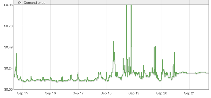
Figure 1.— Example of the pricing of a spot instance over time. Occasionally the rate can meet or exceed the on-demand price, but it is usually much lower. In this example, a bid of $0.24 was safe for a few days from Sep. 15 to Sep. 18.

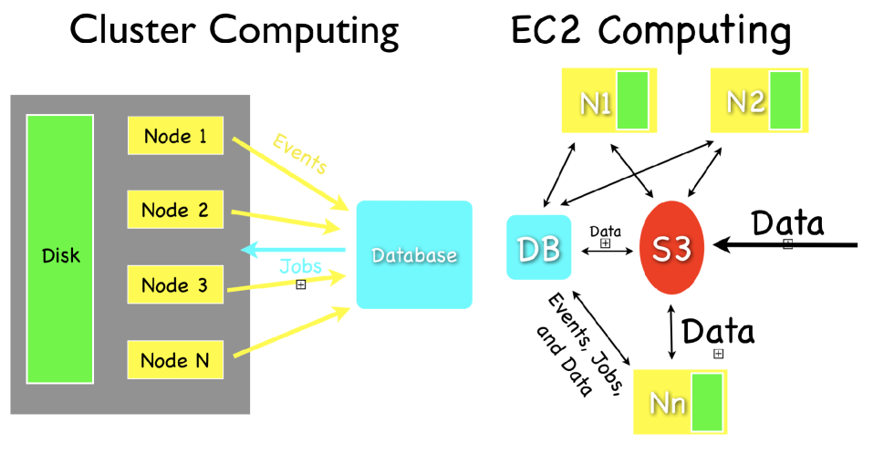
Figure 2.— Left: Schematic of computing on a traditional computing cluster, where all compute nodes share disks and the system has a built-in job scheduler. Right: Schematic of how one replicates a similar system on a computing cloud, where data must be shared between nodes through a common storage system that is not mounted directly to the machines.

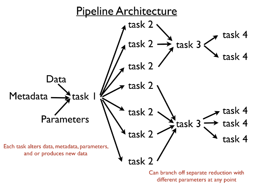
Figure 3.— Schematic of our pipeline architecture, where events start tasks, which then produce more events to complete the analysis.

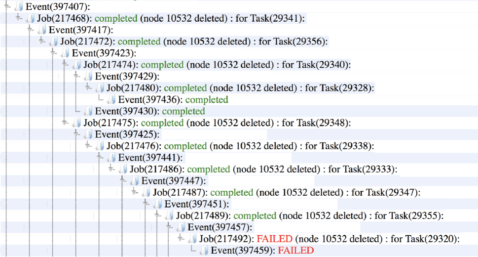
Figure 4.— Example of a pipeline monitoring page. This kind of display makes is simple to find failed jobs, such as 217492 in this example. Then the user can quickly find and investigate problems.

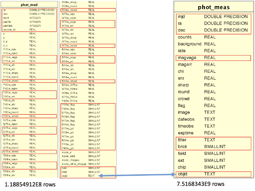
Figure 5.— Entity relationship diagram for the PHAT database tables. The phot_mod table contains the average photometric measurements per object, with 88 columns of measurements and $>$118 million rows, one object per row. The phot_meas table contains all of the single epoch measurements for all of the objects, with 24 columns and $>$7.5 billion rows, one measurement per row. Columns that contain indices in the database are outlined by red boxes, while the tables may be joined on the objid column, the primary key of the tables.

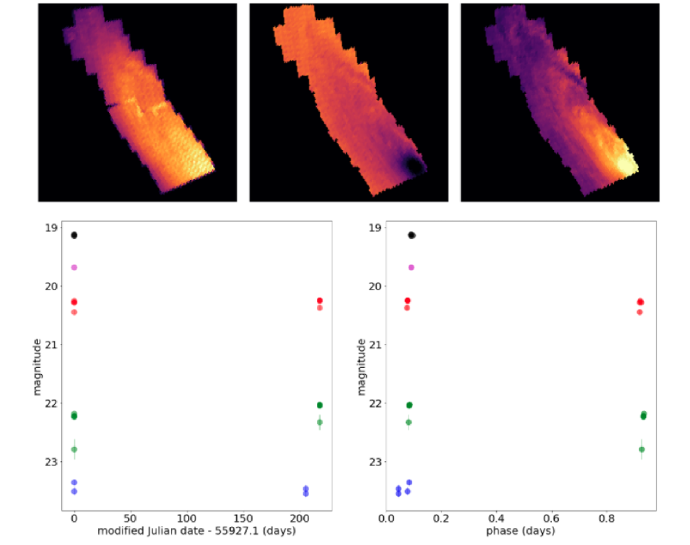
Figure 6.— Figures from our PHAT example Jupyter notebook. Top row: maps of the object density (left), mean magnitude (middle) and mean color (right) obtained by issuing queries to the phat_mod table and aggregating by HEALPix (NSIDE=4096) index. The queries run quickly, allowing efficient exploration of mean quantities of all 118 million objects. Bottom row: the time series (left) and period-folded light curve (right) of the Cepheid variable V5343 (Wagner-Kaiser et al., 2015) from a query of the single epoch phot_meas table.

9. Appendix: Updated Tools for Cloud Computing

Our photometry pipeline infrastructure has proven to be a highly productive and durable science enabling tool over the past decade. However, it highlights features available since $\sim$2009. Our system is now nearly 10 years old, and there are more services available to simplify the creation of such a pipeline. For example, AWS features now include automatic scaling of worker instance numbers, fault tolerance (recovery, re-run of failed jobs) and computational load balancing across a fleet of spot instances. If we were to build a master-worker pipeline today, we would likely use new tools made available by the cloud service providers. Here we discuss some of the newer AWS applications.

For some purposes, off-the-shelf cloud computing solutions from commercial vendors can replicate the capabilities of our pipeline with less development effort. For example, one can now use AWS Batch (and similar services from other cloud services). This service requires the users to upload raw data, analysis scripts and compiled binaries to AWS S3 storage along with a AWS Cloud Formation (JSON format) configuration file describing their computational requirements. The processing is then efficiently executed using the minimum amount of resources needed only for the duration that they are needed. This model is similar to batch processing on clusters or supercomputers and is more easily adopted to different platforms. For comparison, utilization of an AWS Elastic Map Reduce (EMR) cluster can utilize more efficient architecture and applications available on the Hadoop platform (e.g., Presto / Hive QL instead of SQL, Apache Spark for distributed processing, Apache Hbase for storage etc.) but would require the analysis pipeline to be customized for this platform.

Furthermore, there are now services available that essentially mimic much of the functionality of our pipeline without the need to develop them from scratch. The master webserver itself would be replaced by either AWS Lightsail (easily scalable) or AWS Elastic Beanstalk (more economic), with the pipeline database (jobs, tasks, events etc.) residing on AWS Relational Database Service (RDS). Such a change would remove the need for an on-demand server instance to always be running.

The analysis scripts and compilable code could be managed under AWS CodeCommit version control. These would then be deployed for each worker using AWS CodeBuild on a fleet of AWS Lambda (for small,quick task) and AWS EC2 (for processor intensive tasks such as running DOLPHOT) instances accessing AWS Elastic Block Storage (EBS, only accessible by individual instances) or Elastic File System (EFS, networked file systems can accessible by multiple instance or remotely). Raw and processed images along with photometry tables can be marshaled to/from STScI archives and AWS S3/ECS/EFS disks by the AWS Data Pipeline.

Potentially, even the data serving could be put on a cloud service. For example, the photometry tables can be put into searchable AWS Aurora databases using AWS Glue hosted on AWS Redshift that can be queried using AWS,Athena and analyzed (e.g., for variability or anomalies) using AWS Machine Learning (ML) and AWS Artificial Intelligence (AI) tools. However, this kind of service would require a budget to host, unlike the free services supplied by the NOAO Data Lab or the MAST High Level Science Products.

We would like to emphasize that our mention of various AWS offerings by name is merely due to our greater familiarity with this particular cloud service provider. Similar applications from other reputable cloud vendors or through open-source applications (e.g., Openstack Kubernetes) are likely to be just as suitable, but inventorying the cloud marketplace is beyond the scope of this work. Before deciding to use cloud resources for data analysis needs, it is important to perform some cost benefit analysis to determine that it will be beneficial in the long term. We have found it beneficial when one needs many instances occasionally over many years, since purchased computers may sit idle, become obsolete, and lose their warranties over these timescales.

References

- Abolfathi et al. (2017) Abolfathi, B., et al. 2017, ArXiv e-prints, 1707.09322
- Aihara et al. (2011) Aihara, H., et al. 2011, ApJS, 193, 29
- Bobylev & Bajkova (2017) Bobylev, V. V., & Bajkova, A. T. 2017, Astronomy Letters, 43, 559
- Bonanos et al. (2003) Bonanos, A. Z., Stanek, K. Z., Sasselov, D. D., Mochejska, B. J., Macri, L. M., & Kaluzny, J. 2003, AJ, 126, 175
- Fitzpatrick et al. (2016) Fitzpatrick, M. J., et al. 2016, in Proc. SPIE, Vol. 9913, Software and Cyberinfrastructure for Astronomy IV, 99130L
- Fitzpatrick et al. (2014) Fitzpatrick, M. J., et al. 2014, in Proc. SPIE, Vol. 9149, Observatory Operations: Strategies, Processes, and Systems V, 91491T
- Gaudet et al. (2010) Gaudet, S., et al. 2010, in Proc. SPIE, Vol. 7740, Software and Cyberinfrastructure for Astronomy, 77401I
- Ivezić et al. (2007) Ivezić, Ž., et al. 2007, AJ, 134, 973
- Ivezic et al. (2008) Ivezic, Z., et al. 2008, ArXiv e-prints, 0805.2366
- Kaluzny et al. (1999) Kaluzny, J., Mochejska, B. J., Stanek, K. Z., Krockenberger, M., Sasselov, D. D., Tonry, J. L., & Mateo, M. 1999, AJ, 118, 346
- Kaluzny et al. (1998) Kaluzny, J., Stanek, K. Z., Krockenberger, M., Sasselov, D. D., Tonry, J. L., & Mateo, M. 1998, AJ, 115, 1016
- Kleinman et al. (2013) Kleinman, S. J., et al. 2013, ApJS, 204, 5
- Koposov & Bartunov (2006) Koposov, S., & Bartunov, O. 2006, in Astronomical Society of the Pacific Conference Series, Vol. 351, Astronomical Data Analysis Software and Systems XV, ed. C. Gabriel, C. Arviset, D. Ponz, & S. Enrique, 735
- Kurtz et al. (2000) Kurtz, M. J., Eichhorn, G., Accomazzi, A., Grant, C. S., Murray, S. S., & Watson, J. M. 2000, A&AS, 143, 41
- LSST Science Collaboration et al. (2009) LSST Science Collaboration, et al. 2009, ArXiv e-prints
- Ochsenbein et al. (2000) Ochsenbein, F., Bauer, P., & Marcout, J. 2000, A&AS, 143, 23
- Plante (2007) Plante, R. 2007, in Astronomical Society of the Pacific Conference Series, Vol. 382, Astronomical Society of the Pacific Conference Series, ed. M. J. Graham, M. J. Fitzpatrick, & T. A. McGlynn, 381
- Salim et al. (2016) Salim, S., et al. 2016, ApJS, 227, 2
- Shen et al. (2011) Shen, Y., et al. 2011, ApJS, 194, 45
- Spergel et al. (2013) Spergel, D., et al. 2013, ArXiv e-prints
- Stanek et al. (1998) Stanek, K. Z., Kaluzny, J., Krockenberger, M., Sasselov, D. D., Tonry, J. L., & Mateo, M. 1998, AJ, 115, 1894
- Stanek et al. (1999) Stanek, K. Z., Kaluzny, J., Krockenberger, M., Sasselov, D. D., Tonry, J. L., & Mateo, M. 1999, AJ, 117, 2810
- Szalay et al. (2001) Szalay, A., Gray, J., Thakar, A., Kunszt, P. Z., Malik, T., Raddick, J., Stoughton, C., & vandenBerg, J. 2001, eprint arXiv:cs/0111015
- Taylor (2005) Taylor, M. B. 2005, in Astronomical Society of the Pacific Conference Series, Vol. 347, Astronomical Data Analysis Software and Systems XIV, ed. P. Shopbell, M. Britton, & R. Ebert, 29
- Tempel et al. (2014) Tempel, E., Stoica, R. S., Martínez, V. J., Liivamägi, L. J., Castellan, G., & Saar, E. 2014, MNRAS, 438, 3465
- Tian et al. (2017) Tian, H.-J., et al. 2017, ApJS, 232, 4
- Wagner-Kaiser et al. (2015) Wagner-Kaiser, R., Sarajedini, A., Dalcanton, J. J., Williams, B. F., & Dolphin, A. 2015, MNRAS, 451, 724
- Wang et al. (2011) Wang, D. L., Monkewitz, S. M., Lim, K., & Becla, J. 2011, in Conference on High Performance Computing Networking, Storage and Analysis - State of the Practice Reports, SC 2011, Seattle, Washington, USA, November 12-18, 2011, 12:1
- Williams (2015) Williams, B. 2015, WINGS: WFIRST Infrared Nearby Galaxy Survey, NASA WFIRST Proposal
- Williams et al. (2014) Williams, B. F., et al. 2014, ApJS, 215, 9
- Yang et al. (2007) Yang, X., Mo, H. J., van den Bosch, F. C., Pasquali, A., Li, C., & Barden, M. 2007, ApJ, 671, 153
- York et al. (2000) York, D. G., et al. 2000, AJ, 120, 1579