Boson-fermion duality in a gravitational background

Abstract

We study the 2+1 dimensional boson-fermion duality in the presence of background curvature and electromagnetic fields. The main players are, on the one hand, a massive complex $|\phi|^{4}$ scalar field coupled to a $U(1)$ Maxwell-Chern-Simons gauge field at level $1$, representing a relativistic composite boson with one unit of attached flux, and on the other hand, a massive Dirac fermion. We show that, in a curved background and at the level of the partition function, the relativistic composite boson, in the infinite coupling limit, is dual to a short-range interacting Dirac fermion. The coupling to the gravitational spin connection arises naturally from the spin factors of the Wilson loop in the Chern-Simons theory. A non-minimal coupling to the scalar curvature is included on the bosonic side in order to obtain agreement between partition functions. Although an explicit Lagrangian expression for the fermionic interactions is not obtained, their short-range nature constrains them to be irrelevant, which protects the duality in its strong interpretation as an exact mapping at the IR fixed point between a Wilson-Fisher-Chern-Simons complex scalar and a free Dirac fermion. We also show that, even away from the IR, keeping the $|\phi|^{4}$ term is of key importance as it provides the short-range bosonic interactions necessary to prevent intersections of worldlines in the path integral, thus forbidding unknotting of knots and ensuring preservation of the worldline topologies.

1 Introduction

Boson-fermion dualities have been investigated for a long time. The earliest version of this type of duality is the bosonization of fermions in 1+1 space-time dimensions [1, 2, 3, 4]. This is a mapping between a massless Dirac (spinor) fermion $\Psi$ and a massless compactified boson $\varphi$, with compactification radius $R=2\pi$,

$$i\bar{\psi}(\not{\partial}+i\not{A})\psi\longleftrightarrow\frac{1}{8\pi}(\partial_{\mu}\varphi)^{2}-\frac{1}{2\pi}\epsilon^{\mu\nu}A_{\mu}\partial_{\nu}\varphi.$$ (1)

$A_{\mu}$ is an external background gauge field, and $\not{\partial}=\gamma^{\mu}\partial_{\mu}$, with $\gamma^{\mu}$ the gamma matrices. The fermionic current maps to

$$j^{\mu}=\bar{\psi}\gamma^{\mu}\psi\longleftrightarrow\frac{1}{2\pi}\epsilon^{\mu\nu}\partial_{\nu}\varphi.$$ (2)

The 1+1 dimensional boson-fermion duality is a mapping at the operator level, e.g. the fermion mass term ${\bar{\psi}}\psi$ maps onto the vertex operator $\cos\varphi$. It is also at the level of the spectrum and at the level of the partition function.

Things get a bit more subtle in 2+1 dimensions. The first hints at the existence of a 2+1 dimensional boson-fermion duality were found when it was discovered that attaching fluxes to particles could transmute their statistics, becoming anyons [5, 6, 7, 8], a concept that has wide and deep applications particularly in the context of the fractional quantum Hall effects [9, 10, 11]. So if one attaches an odd number of units of flux to a boson, one obtains a composite boson with fermionic statistics. Because these early works dealt with non relativistic composite particles, one may wonder how does flux attachment work in the relativistic case. This is a far more subtle question, because if a relativistic boson, e. g. a scalar field, acquires fermionic statistics under the attachment of an odd number of units of flux, it would give rise to a relativistic fermion. Relativistic fermions are spinors, so now one would have to understand how a relativistic scalar field transmutes into a relativistic spinor Fermi field.

It was Polyakov who first proposed the boson-fermion duality for relativistic massive fields in 2+1 dimensions [12]. He showed that the propagator of a massive free complex scalar field, coupled to a dynamical $U(1)$ Chern-Simons (CS) field [13, 14] at level 1, maps to the propagator of a massive Dirac fermion. The CS field is responsible for the flux attachment, the level 1 corresponding to one unit of flux. Polyakov’s duality reads

$$i\bar{\psi}\not{\partial}\psi+m\bar{\psi}\psi\longleftrightarrow|(\partial_{\mu}+ia_{\mu})\phi|^{2}-m^{2}|\phi|^{2}+\frac{1}{4\pi}\epsilon^{\mu\rho\nu}a_{\mu}\partial_{\rho}a_{\nu}.$$ (3)

Polyakov’s result inspired much subsequent work, most of which focused on the role of different regularization schemes and the associated problem of the framing of knots [15, 16, 17, 18, 19, 20, 21, 22, 23]. However, aspects of Polyakov’s mapping are puzzling. First, if one tries to extend the duality of Eq. (3) by minimally coupling the theories at both sides to a background U(1) gauge field and curvature, one finds that Eq. (3) maps theories with different anomalies: on one side we have a Dirac fermion with a parity anomaly [24, 25, 26, 27, 28, 29], and on the other side a CS gauge field with a framing anomaly [30, 31]. The existence of non matching anomalies presents an obstruction for the duality to be realized, as it stands, as an exact mapping between partition functions. Second, the duality relies on a topological property of Wilson loops in the CS theory: closed worldline configurations are classified in terms of a topological invariant called Gauss’s linking number [32], which counts the number of loops of one worldline around another. If the scalar field is non interacting, then there is no interaction between worldlines and nothing would prevent them to be unknotted, so the topology of the configurations of worldlines would not be preserved. And third, Polyakov’s duality is seemingly valid only for massive free scalar fields. In particular, it cannot be valid in the massless theory whose behavior is controlled by the Wilson-Fisher fixed point. This has come back to focus with the recent works on conjectured CS-matter-dualities in 2+1 dimensions [33, 34, 35, 36, 37, 38, 39, 40, 41, 42, 43, 44, 45, 46, 47, 48, 49, 50, 51]. Notice that the field content of Polyakov’s 2+1-dimensional bosonization duality, Eq.(3), and the 1+1-dimensional bosonization duality, Eq.(1), are quite different: the 1+1-dimensional scalar field $\varphi$ is real and compact and should be regarded as a (failed) Goldstone boson, while Polyakov’s is a non-compact complex scalar field $\phi$. In this sense the analogy is between the 2+1 dimensional complex boson and the vertex operators of the comapctified 1+1 dimensional real boson.

A different perspective on 2+1-dimensional dualities was introduced in the work of Fradkin and Kivelson [52] who introduced a loop model to describe the quantum fluctuations of a system with flux-attachment. In this model, originally introduced as a model of a putative quantum critical point for the quantum Hall plateau transitions, the quantum theory is represented by the closed worldlines of particles and holes (antiparticles). Key to this construction is the assumption that the loops cannot intersect, which always holds for interacting scalar fields below four space-time dimensions. Flux attachment was implemented by demanding that the action of a configuration of loops has an imaginary part proportional to the linking number of the configuration (which is a stable concept if the loops cannot intersect). By imposing that the parity-even part of the action scales in the same way as the imaginary part, Ref. [52] showed that the partition function is invariant under an extended duality in the absence of background gauge fields, and it is covariant under the extended duality in the presence of background gauge fields.

Ref. [52] ignored the self-linking of the worldlines, which led to the existence of an exact invariance under periodic changes of the statistical angle and a full $SL(2,\mathbb{Z})$ exact symmetry. In a recent and separate paper Goldman and one of us [53] has reexamined the issue of the existence of an exact periodicity in asymptotically massless models with Lorentz invariance, and showed that the duality can be implemented consistently, although the existence of fractional spin is generic and, hence, exact periodicity does not hold. Therefore, although loop models can be regarded as a UV completion of the conjectured CS-matter-dualities, extended $SL(2,\mathbb{Z})$ invariance is not generally allowed as an exact symmetry of a partition function. Ref. [53] showed that loop representations can be used to make Polyakov’s duality consistent with the parity anomaly for background electromagnetic fields, and used loop models to check the conjectured web of dualities [36, 35].

On a separate track, in the 1990s other versions of bosonization in 2+1 dimensional relativistic theories were also introduced [54, 55, 56, 57]. These theories use the parity anomaly to map the effective low energy action of conserved currents of theories of massive Dirac fermions to a U(1) Chern-Simons gauge theory. The bosonization rule reads

$$j_{\mu}\leftrightarrow\frac{1}{2\pi}\epsilon_{\mu\nu\lambda}\partial^{\nu}a^{\lambda}$$ (4)

where $j_{\mu}$ is the fermionic current and $a_{\mu}$ is the Chern-Simons gauge field. Notice that this equation has a similar form to Eq. (2). In particular, it relates the fermionic density to the gauge flux. In this sense it is an electric-magnetic duality, and resembles the particle-vortex duality of Refs. [58, 59, 60]. This fermion-gauge duality was recently used to derive an effective hydrodynamic gauge theory of topological insulators [61, 62].

Recently, largely inspired on previous results valid in the large-$N$ limit of fermionic and bosonic theories coupled to Chern-Simon gauge fields [33, 34], it was conjectured [36, 35] that the IR version of the boson-fermion duality maps a massless Dirac fermion to a (strongly) interacting gauged complex scalar field at its Wilson-Fisher fixed point, coupled to a level 1 Chern-Simons gauge field,

$$i\bar{\psi}(\not{\partial}+i\not{A})\psi\longleftrightarrow|(\partial_{\mu}+ia_{\mu})\phi|^{2}-\lambda|\phi|^{4}+\frac{1}{4\pi}\epsilon^{\mu\rho\nu}a_{\mu}\partial_{\rho}a_{\nu}+\frac{1}{2\pi}\epsilon^{\mu\rho\nu}a_{\mu}\partial_{\rho}A_{\nu}.$$ (5)

The validity of this mapping relies on the identification of operators on both sides. In particular, the fermionic current of the left hand side is identified with the gauge flux of the right hand side, in agreement with Eq. (4). Very recently, a proof of this duality at the partition function level has been achieved by using an exact UV correspondence on the lattice [63]. The mapping of Eq. (5) applies in two distinct physical settings, each with different properties and symmetries. One is a theory of Dirac fermions in 2+1 dimensions. In that case, if the theory is defined with a gauge-invariant UV regularization, a time-reversal breaking counterterm of the form $\pm\frac{1}{8\pi}\epsilon_{\mu\nu\lambda}A^{\mu}\partial^{\nu}A^{\lambda}$ (the sign depends on the choice of regularization) should be added to the left hand side of the mapping of Eq. (5) to account for the time-reversal (or parity) anomaly [24, 64]. On the other hand, a manifestly time-reversal invariant theory is possible if the 2+1 dimensional theory is the boundary of a 3+1 dimensional bulk whose effective action is a U(1) gauge theory with a $\theta=\pi$ term, which cancels the parity (or time-reversal) anomaly of the boundary fermions [35].

A comparison of Polyakov’s duality, Eq. (3), with the duality of Eq. (5) suggests that they are not quite consistent with each other. To begin with, in Eq. (3) the complex scalar field is free whereas in Eq. (5) it is interacting and tuned to the (non-trivial) Wilson-Fisher fixed point. Since the fermionic side of Eq. (3) has a mass term it is more relevant to make the comparison with the massive version of Eq. (5). In this case, it was noted in Refs. [36, 35] that the mapping depends on the sign of the fermionic mass. For one sign of the mass term and one choice of regularization, the fermionic theory is in a topological non-trivial phase and maps onto a massive interacting complex scalar in its unbroken (symmetric) phase. This case is consistent with Polyakov’s. However for the opposite sign of the mass, the fermionic theory is trivial and the dual scalar theory is in its broken (Higgs) phase. As it stands, this case cannot be described by Polyakov’s mapping. We will see that there is a way to reconcile these apparent discrepancies.

References [36, 35] used the duality of Eq. (5) as the building block to derive other mappings, arriving to a whole web of dualities in 2+1 dimensions. One of these derived dualities is a map between two Dirac fermions, which was first proposed in refs. [65, 66, 67]. This fermion-fermion duality reads

$$i\bar{\psi}(\not{\partial}+i\not{A})\psi\longleftrightarrow i\bar{\chi}(\not{\partial}+i\not{a})\chi+\frac{1}{4\pi}\epsilon^{\mu\rho\nu}a_{\mu}\partial_{\rho}A_{\nu}.$$ (6)

where the $\chi$ fermions on the right hand side (r.h.s) are non-local respect to the $\psi$ fermions of the left hand side (l.h.s) and act on different Hilbert spaces. The dual Dirac theory of the r.h.s. of Eq. (6) has been related [66, 68, 69] to the bulk electric-magnetic duality of a three dimensional topological insulator [70, 71, 72, 73], while a derivation of the fermion-fermion duality from a wire construction has also appeared in the literature [74, 75]. This fermionic mapping has been used to construct a particle-hole symmetric theory of the half-filled Landau level [65], and all known surface states of the three dimensional topological insulator have been also successfully accessed from the dual Dirac fermion [67].

In this work we re-examine Polyakov’s duality as an exact mapping between partition functions, studying it’s validity in the presence of background metric (curvature), and also gauge fields, and giving an answer to the questions and puzzles stated above. Apart from contributing to the fundamental understanding of the boson-fermion duality, our work opens the door to the study of gravitational responses of relativistic composite particles. For non relativistic composite particles, gravitational responses have been widely studied in the context of the fractional quantum Hall effect [76, 77, 78, 79, 80, 81, 82, 83, 84]. These include thermal responses like the thermal Hall effect [85, 86, 87, 88, 89], which can be related to responses to a gravitational potential by Luttinger’s formalism [90, 91, 92], and geometric responses like the Hall viscosity [93, 94, 78, 95, 96, 77, 97, 98, 99, 80, 100, 101], which are related to the way the fluid couples to geometric properties of the two-dimensional surface on which it moves.

The layout of the paper is as follows. In section 2 we compute the effective action of a relativistic composite boson, in the presence of background curvature and electromagnetic field, and express it as a worldline path integral. In section 3 we apply an analogous procedure to a Dirac fermion. In section 4 we compare the effective actions derived in the previous two sections, and obtain the boson-fermion duality when the bosonic and fermionic theories are both in the trivial and the topological insulating phases. Section 5 is devoted to the conclusions. In order to easing the reading of the manuscript, some derivations and technicalities have been left as appendices.

2 Partition function for the relativistic composite boson

Let us start with the three dimensional action for a complex $|\phi|^{4}$ scalar field in a curved background with Minkowski metric signature, minimally coupled to a $U(1)$ Maxwell-CS gauge field $a_{\mu}$ and to a background field $A_{\mu}$, with $\mu=1,2,3$, and with a conformal coupling to the Ricci scalar curvature $R$, [102, 103, 104, 105]

$$S_{scalar+flux}= \int d^{3}x\sqrt{g}\left[\big{|}D_{\mu}(a,A)\phi\big{|}^{2}-\Big{(}\frac{R}{4}+m^{2}\Big{)}|\phi|^{2}-\lambda|\phi|^{4}\right]+S_{GF}$$

$$S_{GF}= -\frac{1}{4e}\int d^{3}x\sqrt{g}\,F^{2}(a)+CS_{a},$$ (7)

where $D_{\mu}(a,A)=\partial_{\mu}+ia_{\mu}+iA_{\mu}$, $|D_{\mu}\phi|^{2}=g^{\mu\nu}(D_{\mu}\phi)^{*}D_{\nu}\phi$, $F^{2}=g^{\mu\rho}g^{\nu\gamma}F_{\mu\nu}F_{\rho\gamma}$, and $F_{\mu\nu}(a)=\partial_{\mu}a_{\nu}-\partial_{\nu}a_{\mu}$. $CS_{a}$ is

$$CS_{a}=\frac{1}{4\delta}\int d^{3}x\epsilon^{\mu\rho\nu}a_{\mu}\partial_{\rho}a_{\nu},$$ (8)

where we choose the statistical angle to be $\delta=\pi$, so that we have a level 1 CS term. We included a Maxwell $F^{2}$ term for $a_{\mu}$ which, as we will see, will serve as an UV regulator. We can introduce an auxiliary scalar field $\sigma$ and write

$$S_{scalar+flux}=\int d^{3}x\sqrt{g}\left[\big{|}D_{\mu}(a,A)\phi\big{|}^{2}-\Big{(}\frac{R}{4}+m^{2}+2i\sqrt{\lambda}\,\sigma\Big{)}|\phi|^{2}-\sigma^{2}\right]+S_{GF},$$ (9)

such that integrating it out we recover the action (7). The partition function reads

$$Z_{scalar+flux}=\int D\phi^{*}D\phi D\sigma Da_{\mu}\,e^{iS_{scalar+flux}}.$$ (10)

Integrating out $\phi$ one obtains, after a Wick rotation $t\rightarrow-it$ and using the identity $\ln\det=\mathrm{tr}\ln$ ,

$$Z_{scalar+flux}=\int D\sigma Da_{\mu}\,e^{-\Gamma^{\prime}}\,e^{-\int d^{3}x\,\sigma^{2}}\,e^{-S_{GF}},$$ (11)

with the effective action $\Gamma^{\prime}$

$$\Gamma^{\prime}=\mathrm{tr}\ln\Big{[}-\frac{1}{\sqrt{g}}D_{\mu}(a,A)\sqrt{g}\,g^{\mu\nu}D_{\nu}(a,A)+\frac{R}{4}+m^{2}+2i\sqrt{\lambda}\,\sigma\Big{]}.$$ (12)

Now the metric $g^{\mu\nu}$ has euclidean signature. Following appendix A.1, $\Gamma^{\prime}$ can be written as a path integral over worldlines

$$-\Gamma^{\prime}=\int_{\epsilon}^{\infty}dt\,t^{-1}\,\int DX^{\mu}\,e^{-\int_{0}^{t}ds\big{(}\frac{1}{4}\dot{X}^{2}-ia_{\mu}\dot{X}^{\mu}-iA_{\mu}\dot{X}^{\mu}+\frac{R}{4}+m^{2}+2i\sqrt{\lambda}\,\sigma\big{)}},$$ (13)

with $X_{\mu}(t)=X_{\mu}(0)$ and where we introduced a cut-off $\epsilon$.

2.1 Integrating out the Chern-Simons field

Now we proceed to integrate out the CS field. We can write

$$Z_{scalar+flux}=\int D\sigma Da_{\mu}\,e^{-\Gamma^{\prime}}\,e^{-\int d^{3}x\,\sigma^{2}}\,e^{-S_{GF}}$$

$$=Z_{GF}\int D\sigma\,e^{-\int d^{3}x\,\sigma^{2}}\left\langle\exp\Big{[}\int_{\epsilon_{s}}^{\infty}dt\,t^{-1}\,DX^{\mu}\,e^{-\int_{0}^{t}ds\big{(}\frac{1}{4}\dot{X}^{2}-iA_{\mu}\dot{X}^{\mu}+\frac{R}{4}+m^{2}+2i\sqrt{\lambda}\,\sigma\big{)}}e^{i\int_{0}^{t}ds\,\dot{X}^{\mu}a_{\mu}}\Big{]}\right\rangle_{CS},$$ (14)

where

$$Z_{GF}=\int Da_{\mu}\,e^{-S_{GF}},$$ (15)

and $\langle...\rangle_{CS}$ denotes the expectation value over the CS field

$$\langle...\rangle_{CS}=Z_{GF}^{-1}\int Da_{\mu}\,(...)\,e^{-S_{GF}},$$ (16)

We can write the exponential as a series

$$\left\langle\sum_{n=0}^{\infty}\frac{1}{n!}\Big{(}\int_{\epsilon_{s}}^{\infty}dt\,t^{-1}\,DX^{\mu}\,e^{-\int_{0}^{t}ds\big{(}\frac{1}{4}\dot{X}^{2}-iA_{\mu}\dot{X}^{\mu}+\frac{R}{4}+m^{2}+2i\sqrt{\lambda}\,\sigma\big{)}}e^{i\int_{0}^{t}ds\,\dot{X}^{\mu}a_{\mu}}\Big{)}^{n}\right\rangle_{CS}$$

$$=1+\sum_{n=1}^{\infty}\frac{1}{n!}\left(\prod_{i=1}^{n}\int_{\epsilon_{s}}^{\infty}dt_{i}\,t_{i}^{-1}\,DX^{\mu}_{i}\,e^{-\int_{0}^{t_{i}}ds\big{(}\frac{1}{4}\dot{X}^{2}_{i}-iA_{\mu}\dot{X}^{\mu}_{i}+\frac{R}{4}+m^{2}+2i\sqrt{\lambda}\,\sigma\big{)}}\right)\Big{\langle}\prod_{i=1}^{n}e^{i\int_{0}^{t_{i}}ds\,\dot{X}_{i}^{\mu}a_{\mu}}\Big{\rangle}_{CS}.$$ (17)

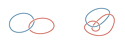
Figure 1: Linking of two worldlines. The Gauss’s linking numbers of the left and right configurations are $\pm 1$ and $\pm 2$, respectively (the sign depends on the relative orientation of the worldlines).

Integrating out the scalar field $\sigma$ we get (up to a multiplicative constant)

$$Z_{scalar+flux}\,Z_{GF}^{-1}= 1+\sum_{n=1}^{\infty}\frac{1}{n!}\left(\prod_{i=1}^{n}\int_{\epsilon_{s}}^{\infty}dt_{i}\,t_{i}^{-1}\,DX^{\mu}_{i}\,e^{-\int_{0}^{t_{i}}ds\big{(}\frac{1}{4}\dot{X}^{2}_{i}-iA_{\mu}\dot{X}^{\mu}_{i}+\frac{R}{4}+m^{2}\big{)}}\right)$$

$$\times\left(\prod_{i,j=1}^{n}e^{-\lambda\int_{0}^{t_{i}}ds\int_{0}^{t_{j}}ds^{\prime}\,\delta(X_{i}-X_{j})}\right)\,\Big{\langle}\prod_{i=1}^{n}e^{i\int_{0}^{t_{i}}ds\,\dot{X}_{i}^{\mu}a_{\mu}}\Big{\rangle}_{CS}.$$ (18)

Hence we obtain the well known result that the $\phi^{4}$ interaction amounts to a short range repulsive interaction between worldlines [106, 107, 108]. Such a term suppresses intersecting worldline configurations, which is key as we will see below.

We can now proceed to compute the expectation value of the product of Wilson loops (in the Feynman gauge) [12, 18]

$$\Big{\langle}\prod_{i=1}^{n}e^{i\int_{0}^{t_{i}}ds\,\dot{X}_{i}^{\mu}a_{\mu}}\Big{\rangle}_{CS}=\Big{\langle}\prod_{i=1}^{n}e^{i\oint_{C_{i}}dx^{\mu}a_{\mu}}\Big{\rangle}$$

$$=\prod_{i,j=1}^{n}\exp\left\{\frac{e^{2}}{8\pi}\oint_{C_{i}}dx^{\mu}\oint_{C_{j}}dy^{\nu}\Big{[}i\epsilon_{\mu\nu\rho}\frac{r^{\rho}}{\mu r^{3}}\big{(}1-(1+\mu r)e^{-\mu r}\big{)}-\delta_{\mu\nu}\frac{e^{-\mu r}}{r}\Big{]}\right\},$$ (19)

where $r=|x-y|$, and $\mu=e^{2}/2\delta$ (in our case $\delta=\pi$) has the effect of screening the interactions between worldlines, down to the non-local linking number. Here the Maxwell term acts as an UV regulator, with coupling constant $e$. If $C_{i}=C_{j}$ we get the expectation value of a single Wilson loop

$$\exp\left\{\frac{e^{2}}{8\pi}\oint_{C_{i}}dx^{\mu}\oint_{C_{i}}dy^{\nu}\Big{[}i\epsilon_{\mu\nu\rho}\frac{r^{\rho}}{\mu r^{3}}\big{(}1-(1+\mu r)e^{-\mu r}\big{)}-\delta_{\mu\nu}\frac{e^{-\mu r}}{r}\Big{]}\right\}\equiv\Big{\langle}e^{i\oint_{C_{i}}dx^{\mu}a_{\mu}}\Big{\rangle}_{CS},$$ (20)

which we will look at more carefully in the next two sections. For the case of distinct closed loops $C_{i}$, $C_{j}$, and in the limit $e\rightarrow\infty$ we get

$$\exp\left[\frac{1}{4}\oint_{C_{i}}dx^{\mu}\oint_{C_{j}}dy^{\nu}i\epsilon_{\mu\nu\rho}\frac{r^{\rho}}{r^{3}}\right]=\pi L(C_{i},C_{j}).$$ (21)

$L(C_{i},C_{j})$ is the Gauss linking number of $C_{i}$ and $C_{j}$ [32]. It is a topological invariant which takes integer values (see figure 1). However, $L(C_{i},C_{j})$ is well defined only if $C_{i}$ and $C_{j}$ do not intersect. But we have seen that the $|\phi|^{4}$ self-interaction provides Dirac delta type interactions between worldlines, such that configurations with intersections are suppressed. Or in other words, the $|\phi|^{4}$ term is key to prevent links and knots from being unlinked and unknotted, preserving their topology. We then have

$$\Big{\langle}\prod_{i=1}^{n}e^{i\oint_{C_{i}}dx^{\mu}a_{\mu}}\Big{\rangle}_{CS}=\left(\prod_{i=1}^{n}\Big{\langle}e^{i\oint_{C_{i}}dx^{\mu}a_{\mu}}\Big{\rangle}_{CS}\right)\exp\Big{(}i\pi\sum_{i<j}2L(C_{i},C_{j})\Big{)}$$

$$=\prod_{i=1}^{n}\Big{\langle}e^{i\oint_{C_{i}}dx^{\mu}a_{\mu}}\Big{\rangle}_{e\rightarrow\infty},$$ (22)

where we took the limit $e\to\infty$ (where the Maxwell term is formally absent) and where, in the summation over $i,j$, intersecting curves are excluded. In these expressions the remaining expectation values of the gauge field involve only one loop at a time. We will show below that these factors play an important role.

We see then that the expectation value of the product of Wilson loops factorizes. It is important to note that this is only the case if the statistical angle is $\delta=n\pi$, $n\in\mathbb{Z}$. For other values of $\delta$, the exponential $\exp(i\delta\sum_{i<j}2L)$ would induce interactions between Wilson loops. For the partition function we get, in the limit $e\rightarrow\infty$,

$$Z^{e\rightarrow\infty}_{scalar+flux}\,Z_{CS}^{-1} =$$ (23)

$$\int D\sigma\,e^{-\int d^{3}x\,\sigma^{2}} \exp\Big{[}\int_{\epsilon_{s}}^{\infty}dt\,t^{-1}\,DX^{\mu}\,e^{-\int_{0}^{t}ds\big{(}\frac{1}{4}\dot{X}^{2}-iA_{\mu}\dot{X}^{\mu}+\frac{R}{4}+m^{2}+2i\sqrt{\lambda}\,\sigma\big{)}}\Big{\langle}e^{i\int_{0}^{t}ds\,\dot{X}^{\mu}a_{\mu}}\Big{\rangle}\Big{]},$$ (24)

where we have taken the limit $Z^{e\rightarrow\infty}_{GF}=Z_{CS}$, with $Z_{CS}$ being the partition function for the pure CS theory, and where we restored the functional integration over $\sigma$. We will express these results as a path integral over the $\sigma$ fields,

$$Z^{e\rightarrow\infty}_{scalar+flux}=Z_{CS}\int D\sigma\,e^{-\int d^{3}x\,\sigma^{2}}\,e^{-\Gamma_{scalar+flux}},$$ (25)

where the effective action $\Gamma_{scalar+flux}$ is

$$-\Gamma_{scalar+flux}=\int_{\epsilon}^{\infty}dt\,t^{-1}\,\int DX^{\mu}\,e^{-\int_{0}^{t}ds\big{(}\frac{1}{4}\dot{X}^{2}-iA_{\mu}\dot{X}^{\mu}+\frac{R}{4}+m^{2}+2i\sqrt{\lambda}\,\sigma\big{)}}\,\Phi(C),$$ (26)

with $\Phi(C)$ the expectation value of the Wilson loop

$$\Phi(C)=\big{\langle}e^{i\oint_{C}dx^{\mu}a_{\mu}}\big{\rangle}_{e\rightarrow\infty}.$$ (27)

2.2 The Wilson loop in flat space-time

As a first step, let us compute the expectation value of the Wilson loop when space-time is flat

$$\Phi_{flat}(C)=\lim_{e\rightarrow\infty}\,\exp\left\{\frac{e^{2}}{8\pi}\oint_{C}dx^{a}\oint_{C}dy^{b}\Big{[}i\,\epsilon_{abc}\frac{r^{c}}{\mu r^{3}}\big{(}1-(1+\mu r)e^{-\mu r}\big{)}-\delta_{ab}\frac{e^{-\mu r}}{r}\Big{]}\right\}.$$ (28)

By doing $r<<1/\mu$ we see that the first term goes as $\mu\epsilon_{abc}r^{c}/r$, so that the only singularity lives entirely in the screened Coulomb term $e^{-\mu r}/r$. Taking the limit $e\rightarrow\infty$ we get

$$\Phi_{flat}(C)=\exp\left[\frac{i}{4}\oint_{C}dx^{a}\oint_{C}dy^{b}\epsilon_{abc}\frac{r^{c}}{r^{3}}\right]=e^{i\pi W_{flat}}.$$ (29)

The integral (29) is finite and equal to the writhe W of the curve C [109]. The writhe depends on the shape of the curve, hence the Wilson loop depends on the metric of space-time. This might seem in contradiction with Witten’s work [30], where he regularized the integral (29) by means of a ‘point splitting’ procedure which yields the result

$$\exp\left[\frac{i}{4}\oint_{C}dx^{a}\oint_{C}dy^{b}\epsilon_{abc}\frac{(r-\epsilon\hat{n})^{c}}{|\bm{r}-\epsilon\hat{\bm{n}}|^{3}}\right]=e^{i\pi SL},$$ (30)

where the unit normal vector $\hat{\bm{n}}$ defines a framing for the curve C. This can be viewed as if the curve is transformed into a ribbon (see figure 2). The integral of Eq.(30) gives a topological invariant called self-linking number (SL), which is an integer and is basically the Gauss’s linking number between the two edges of the ribbon. It depends on the choice of frame $\hat{n}$, and is related to the writhe W by the formula $SL=W+T$, where T is the twist of the ribbon [110].

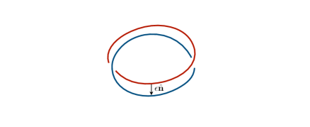
Figure 2: Worldline transformed into a ribbon of self-linking number $SL=1$.

So we have two different regularizations of the Wilson loop: Eq. (29), obtained as the $e\rightarrow\infty$ limit of Eq. (28), which is metric dependent but frame independent, and Eq.(30), obtained from the pure CS theory by doing point splitting, which is topological but frame dependent. This is a manifestation of the framing anomaly of the CS theory [30, 31], which reflects the impossibility of finding a regularization which is topological and frame independent at the same time. The reason definitions of Eqs. (29) and (30) give different results lies in the fact that the limit $\epsilon\rightarrow 0$ is not smooth. The ambiguity in this limit is lost in Eq. (28), where the $F^{2}$ term smoothens the singularity of the CS propagator, and the metric dependent result of Eq. (29) is obtained [18]. This is the correct result in our case, since we are considering the pure CS theory as the $e\rightarrow\infty$ limit of a Maxwell-CS theory. The $F^{2}/4e^{2}$ term in the gauge field Lagrangian plays the role of a UV regulator which is forcing us to quantize the theory in a non topological, but frame invariant way.

Next let us introduce a moving frame $(\bm{e}^{1},\bm{e}^{i})$ along the worldline C (with $i=2,3$) given in parametric form by $X_{a}(s)$, and

$$|\bm{e}^{1}|=|\bm{e}^{i}|=1;\quad e^{1}_{a}=\frac{\dot{X}_{a}}{|\dot{\bm{X}}|}=\epsilon_{abc}\,e^{2}_{b}\,e^{3}_{c}.$$ (31)

The twist T can be defined as [12]

$$T_{flat}=\frac{1}{2\pi}\int_{0}^{t}ds\,\epsilon_{abc}\,e^{1}_{a}\,e^{2}_{b}\,\dot{e}^{2}_{c}.$$ (32)

Following Refs. [12, 111, 19, 112, 113] we can write T, and therefore W through the formula $SL=W+T$, as a Wess-Zumino-Witten (“Berry phase”) term [114, 115] (see appendix B)

$$W_{flat}=\frac{\Omega_{flat}}{2\pi}+SL+\nu.$$ (33)

where the integer $\nu\in\mathbb{Z}$ is the self-winding number of the loop and the Wess-Zumino-Witten action, $\Omega_{flat}$, is

$$\Omega_{flat}=\int_{0}^{1}d\rho\int_{0}^{t}ds\,\epsilon_{abc}\,e^{1}_{a}\,\partial_{\rho}e^{1}_{b}\,\partial_{s}e^{1}_{c}.$$ (34)

Here $\rho\in[0,1]$ is an auxiliary coordinate, and $\bm{e}^{1}$ is extended to $\bm{e}^{1}(t,\rho)$ in such a way that $\bm{e}^{1}(t,0)=\bm{e}_{0}$ and $\bm{e}^{1}(t,1)=\bm{e}^{1}(t)$, with $\bm{e}_{0}$ some constant vector. It turns out that $\Omega_{flat}$ is just the signed area enclosed by the path C on the sphere $S_{2}$, defined by $\bm{e}^{1}:C\rightarrow S_{2}$. Finally, it can be seen that $W_{flat}-\Omega_{flat}/2\pi$ is an odd integer [17, 21] , so that

$$W_{flat}=\frac{\Omega_{flat}}{2\pi}+2n+1,\quad n\in\mathbb{Z},$$ (35)

and the Wilson loop reads

$$\Phi_{flat}(C)=-e^{i\Omega_{flat}/2}.$$ (36)

As a final note, it is instructive to check the frame invariance of the Wilson loop. By doing the clockwise rotation

$$\tilde{\bm{e}}^{2}=\cos\varphi\,\bm{e}^{2}+\sin\varphi\,\bm{e}^{3},\quad\quad\tilde{\bm{e}}^{3}=-\sin\varphi\,\bm{e}^{2}+\cos\varphi\,\bm{e}^{3},$$ (37)

where periodicity demands $\varphi(t)=\varphi(0)+2\pi m$, with $m\in\mathbb{Z}$, the winding number $\nu$ in Eq. (33) is shifted by $\tilde{\nu}=\nu+m$ (see appendix B). At the same time, such a rotation of the frame also shifts the self-linking number: $\tilde{SL}=SL-m$. Therefore the writhe, and by extension the Wilson loop, are frame invariant.

2.3 The Wilson loop in curved space-time

Extending the Wilson loop, in the limit $e\rightarrow\infty$, to curved space-times is quite straight forward. The most obvious way to do it is to start with the definition in terms of the twist of the curve

$$\Phi(C)=e^{i\pi W}=e^{i\pi SL}e^{-i\pi T}.$$ (38)

The extension of the twist to curved spaces is then performed by the substitution $\partial_{s}\rightarrow\dot{X}^{\gamma}\nabla_{\gamma}$, with $\nabla_{\gamma}\xi^{\nu}=\partial_{\gamma}\xi^{\nu}+\Gamma^{\nu}_{\beta\gamma}\xi^{\beta}$, where $\Gamma^{\nu}_{\beta\gamma}$ is the Christoffel symbol. We get

$$T=\frac{1}{2\pi}\int_{0}^{t}ds\,\epsilon_{\mu\rho\nu}\,e^{1\mu}\,e^{2\rho}\,\dot{X}^{\gamma}\nabla_{\gamma}e^{2\nu}.$$ (39)

Using the vielbein postulate

$$\nabla_{\gamma}E^{\nu}_{a}=\partial_{\gamma}E^{\nu}_{a}+\Gamma^{\nu}_{\beta\gamma}E^{\beta}_{a}-\tensor{\omega}{{}_{\gamma}{}_{a}^{b}}E^{\nu}_{b}=0,$$ (40)

with $E^{\nu}_{a}$ the vielbein and $\tensor{\omega}{{}_{\gamma}{}_{a}^{b}}$ the spin connection, we can write

$$\dot{X}^{\gamma}\nabla_{\gamma}e^{2\nu}=\dot{X}^{\gamma}\nabla_{\gamma}(E^{\nu}_{a}e^{2a})=E^{\nu}_{a}\dot{e}^{2a}+e^{2a}\dot{X}^{\gamma}(\partial_{\gamma}E^{\nu}_{a}+\Gamma^{\nu}_{\beta\gamma}E^{\beta}_{a})=E^{\nu}_{a}\dot{e}^{2a}+e^{2a}\dot{X}^{\gamma}\tensor{\omega}{{}_{\gamma}{}_{a}^{b}}E^{\nu}_{b}.$$ (41)

The twist then reads

$$T=T_{flat}+\frac{1}{2\pi}\int_{0}^{t}ds\,e^{2}_{a}\,e^{3}_{b}\,\dot{X}^{\gamma}\,\tensor{\omega}{{}_{\gamma}^{a}{}^{b}},$$ (42)

where we have done $\epsilon_{\mu\rho\nu}\,e^{1\mu}\,e^{2\rho}=e^{3}_{\nu}$, and $T_{flat}$ is the twist in the non-coordinate basis, denoted by Latin indexes. Using the fact that the spin connection is antisymmetric under $a\leftrightarrow b$, we can write $e^{2}_{a}\,e^{3}_{b}=e^{2}_{[a}\,e^{3}_{b]}=\epsilon_{abc}\,e^{1c}/2$, and arrive to

$$T=T_{flat}+\frac{1}{4\pi}\int_{0}^{t}ds\,\dot{X}^{\mu}\,e^{1a}\,\epsilon_{abc}\,\tensor{\omega}{{}_{\mu}^{b}{}^{c}}.$$ (43)

Finally, the expression for the Wilson loop in curved space-time is

$$\Phi(C)=-e^{i\Omega/2}$$ (44)

$$\Omega=\Omega_{flat}-\frac{1}{2}\int_{0}^{t}ds\,\dot{X}^{\mu}e^{1a}\epsilon_{abc}\,\tensor{\omega}{{}_{\mu}^{b}{}^{c}}.$$ (45)

So the Wilson loop divides into two contributions: the Wess-Zumino-Witten term, $\Omega_{flat}$, which is topological and does not depend on the metric, and the spin connection term, which encodes all the information of the background curvature. An alternative derivation in terms of path integrals of one dimensional fermions is given in appendix C.

2.4 Framing anomaly of the free CS theory

Now that we have the Wilson loop, we need to compute the vacuum contribution of the gauge field sector, $Z_{GF}$, which in the limit $e\rightarrow\infty$ is just the partition function for the pure CS theory, $Z_{CS}$. At the classical level, the CS theory is well known to be topological, but this is no longer true when one considers the quantum theory. In the path integral formulation, this means that the integration measure in the partition function is metric dependent. This dependence arises from the need to fix the gauge, which can be done by including gauge fixing terms which do depend on the metric. The calculation of $Z_{CS}$ in a curved background was first done by Witten [30], so here we just recall the result [30, 31, 84]

$$Z_{CS}=\tau^{1/2}\,e^{-i\pi\eta_{g}/2}.$$ (46)

$\tau^{1/2}$ is a topological invariant, the square root of the Ray-Singer analytic torsion [116], which is just a constant multiplicative term. Here $\eta_{g}$ is the eta-invariant [117] of the purely gravitational operator. It is a regularized version of the difference between the number of positive and negative eigenvalues of the Dirac operator. In the special case that our three-dimensional manifold is a boundary of some four-dimensional manifold, then the Atiyah-Patodi-Singer index theorem [117] tells us that [64]

$$\frac{\eta_{g}}{2}=\frac{CS_{g}}{\pi}\,\,\mathrm{mod}\,\mathbb{Z}$$ (47)

Here $CS_{g}$ is the gravitational CS term [13, 14], which in terms of the spin connection is given by

$$CS_{g}=\frac{1}{96\pi}\mathrm{tr}\int d^{3}x\,\epsilon^{\mu\rho\nu}\big{(}\omega_{\mu}\partial_{\rho}\omega_{\nu}+\frac{1}{3}\omega_{\mu}[\omega_{\rho},\omega_{\nu}]\big{)}$$ (48)

For a general three-dimensional manifold, a topological invariant can be constructed by subtracting $CS_{g}$ to the eta-invariant: $\eta_{g}/2-CS_{g}/\pi$. The subtlety is that $CS_{g}$ depends on the choice of frame, so the quantity $\eta_{g}/2-CS_{g}/\pi$ can be defined as a topological invariant of a framed manifold [30, 31]. This is what gives rise to the framing anomaly, because one could think of regulating the theory by adding a counterterm $-CS_{g}$ to make $Z_{CS}$ topological, but this would come with the price of loosing frame invariance.

Finally, from the previous discussion we can set $\eta_{g}/2=CS_{g}$, which is always true up to multiplicative constant terms unimportant for our discussion. We can then write

$$Z_{CS}=e^{-iCS_{g}}.$$ (49)

2.5 Effective action

Putting the previous pieces together, we obtain to the following effective action, in the limit $e\rightarrow\infty$

$$\Gamma_{scalar+flux} =iCS_{g}$$

$$+\int_{\epsilon}^{\infty} dt\,t^{-1}\,\int DX^{\mu}\,e^{-\int_{0}^{t}ds\big{(}\frac{1}{4}\dot{X}^{2}-iA_{\mu}\dot{X}^{\mu}+\frac{i}{4}e^{1a}\epsilon_{abc}\,\tensor{\omega}{{}_{\mu}^{b}{}^{c}}\dot{X}^{\mu}+\frac{R}{4}+m^{2}+2i\sqrt{\lambda}\,\sigma\big{)}}\,e^{i\Omega_{flat}/2}\,.$$ (50)

We have added the contribution of the framing anomaly $iCS_{g}$, so the notation now reads

$$Z^{e\rightarrow\infty}_{scalar+flux}=\int D\sigma\,e^{-\int d^{3}x\,\sigma^{2}}\,e^{-\Gamma_{scalar+flux}}.$$ (51)

3 Partition function for a Dirac fermion

We will now consider a massive Dirac fermion in 2+1 dimensions, and write its effective action as a worldline path integral. The goal is to compare the result with the effective action for the relativistic composite boson. In order to do this, we can write the action of a Dirac fermion as

$$S_{f}=\int d^{3}x\,\sqrt{g}\,\bar{\Psi}\big{(}i\not{D}(A,\omega)-m\big{)}\Psi,$$ (52)

with $\not{D}=\gamma^{\mu}D_{\mu}$, $\gamma^{\mu}$ the Gamma matrices, and

$$D_{\mu}(\omega,A)=\partial_{\mu}+iA_{\mu}+\frac{1}{8}\tensor{\omega}{{}_{\mu}^{a}{}^{b}}[\gamma_{a},\gamma_{b}].$$ (53)

The partition function reads

$$Z_{f}=\int D\bar{\Psi}D\Psi\,\,e^{iS_{f}}=\det\Big{(}\not{D}(A,\omega)+im\Big{)}.$$ (54)

Wick rotating to three-dimensional Euclidean space-time it becomes

$$Z_{f}=e^{-\Gamma_{f}}=\det\Big{(}i\not{D}(A,\omega)+im\Big{)},$$ (55)

where $\not{D}=\sigma^{\mu}D_{\mu}$, with $\sigma^{\mu}$ the Pauli matrices, and the metric is now given in euclidean signature. The covariant derivative reads

$$D_{\mu}(\omega,A)=\partial_{\mu}+iA_{\mu}+\frac{1}{8}\tensor{\omega}{{}_{\mu}^{a}{}^{b}}[\sigma_{a},\sigma_{b}].$$ (56)

We can separate the real and imaginary parts of the effective action as follows

$$\Gamma_{f}=\mathcal{R}(\Gamma_{f})+i\mathcal{I}(\Gamma_{f})=-\ln\big{|}\det\big{(}i\not{D}(A,\omega)+im\big{)}\big{|}-i\,\mathrm{arg}\Big{[}\det(i\not{D}(A,\omega)+im)\Big{]},$$ (57)

where $arg$ denotes the argument. By using the identities $|\det\hat{\mathcal{O}}|^{2}=\det(\hat{\mathcal{O}}^{\dagger}\hat{\mathcal{O}})$ and $\ln\det=\mathrm{tr}\ln$, we get

$$\mathcal{R}(\Gamma_{f})=-\frac{1}{2}\mathrm{tr}\ln\Big{(}-\not{D}^{2}(A,\omega)+m^{2}\Big{)}$$ (58)

$$\mathcal{I}(\Gamma_{f})=-\mathrm{arg}\Big{[}\det(i\not{D}(A,\omega)+im)\Big{]}.$$ (59)

The imaginary part of the effective action breaks time-reversal and parity symmetry. This comes from the fact that, in an orientable space-time $X$ of euclidean signature, the partition function complex conjugates under a time-reversal transformation, which can be implemented by reversing the orientation of $X$ [64].

The imaginary, time-reversal breaking part of the effective action of a Dirac fermion is well known to acquire a term proportional to the combination $-CS_{A}/2-CS_{g}$, the proportionality constant being the sign of the fermion mass [118, 24, 25, 26, 27, 119, 120]. In addition, there is an extra contribution $\mp CS_{A}/2\mp CS_{g}$ due to the parity anomaly [24, 25, 26, 27, 28, 29], the sign depending on the choice of regularization, e.g. if one regularizes using a Pauli-Villars regulator, the sign corresponds to the sign of the regulator mass. Putting the two contributions together one gets

$$\mathcal{I}(\Gamma_{f})=-\big{(}\mathrm{sign}(m)\pm 1\big{)}\Big{(}\frac{CS_{A}}{2}+CS_{g}\Big{)}$$ (60)

Regarding the real part of the effective action, we make use of the Schrödinger-Lichnerowicz formula for the squared Dirac operator

$$-\not{D}^{2}(A,\omega)=-\frac{1}{\sqrt{g}}D_{\mu}(A,\omega)\sqrt{g}\,g^{\mu\nu}D_{\nu}(A,\omega)+\frac{R}{4}-\frac{i}{4}F_{\mu\nu}[\sigma^{\mu},\sigma^{\nu}].$$ (61)

Then, using results of appendix A.1, we can write it as a worldline path integral

$$-2\mathcal{R}(\Gamma_{f})=\mathrm{tr}\ln\big{(}-\not{D}^{2}(A,\omega)+m^{2}\big{)}$$

$$=-\int_{\epsilon}^{\infty}dt\,t^{-1}\,\int DX^{\mu}\,\tilde{\mathrm{tr}}\,\mathcal{P}\,e^{-\int_{0}^{t}ds\big{(}\frac{1}{4}\dot{X}^{2}-iA_{\mu}\dot{X}^{\mu}+F^{*}_{\mu}(A)\sigma^{\mu}+\frac{i}{4}\tensor{\omega}{{}_{\mu}^{a}{}^{b}}\epsilon_{abc}\sigma^{c}\dot{X}^{\mu}+\frac{R}{4}+m^{2}\big{)}},$$ (62)

where the tilde in $\tilde{\mathrm{tr}}$ means the trace is over the spin indices, $\mathcal{P}$ denotes path ordering, and $F^{*}_{\mu}(A)$ is the Hodge dual of the background field strength $F^{*}_{\mu}(A)=\epsilon_{\mu\rho\nu}F^{\rho\nu}(A)/2$.

To compute the trace, we follow Ref.[121] and parametrize the states by picking the “time” direction, $x_{3}$, and “boost” eigenstates of $\sigma^{3}$ to eigenstates of $e^{1}_{\mu}\sigma^{\mu}$: $e^{1}_{\mu}\sigma^{\mu}\,|\bm{e}^{1},+\rangle=|\bm{e}^{1},+\rangle$, $e^{1}_{\mu}\sigma^{\mu}\,|\bm{e}^{1},-\rangle=-|\bm{e}^{1},-\rangle$. The trace of a spin operator then reads $\tilde{\mathrm{tr}}\,\hat{\mathcal{O}}=\langle\bm{e}^{1},+|\hat{\mathcal{O}}|\bm{e}^{1},+\rangle+\langle\bm{e}^{1},-|\hat{\mathcal{O}}|\bm{e}^{1},-\rangle$. For an operator of the form $\hat{\mathcal{O}}=e^{i\int_{0}^{t}ds\frac{1}{2}B_{\mu}\sigma^{\mu}}$, the quantity $\langle\bm{e}^{1},\pm|\hat{\mathcal{O}}|\bm{e}^{1},\pm\rangle$ has been evaluated in the context of coherent state path integrals for non relativistic spinning particles [122, 123, 124, 125, 126]

$$\langle\bm{e}^{1},\pm|e^{i\int_{0}^{t}ds\frac{1}{2}B_{\mu}\sigma^{\mu}}|\bm{e}^{1},\pm\rangle=e^{\pm i\int_{0}^{t}ds\frac{1}{2}B_{\mu}e^{1\mu}}e^{\pm\frac{i}{2}\Omega_{flat}}.$$ (63)

Using this result, we get for $\mathcal{R}(\Gamma_{f})$

$$\mathcal{R}(\Gamma_{f}) =\int_{\epsilon}^{\infty}dt\,t^{-1}\,\int DX^{\mu}\,e^{-\int_{0}^{t}ds\big{(}\frac{1}{4}\dot{X}^{2}-iA_{\mu}\dot{X}^{\mu}+\frac{R}{4}+m^{2}\big{)}}$$

$$\times\cos\Big{[}\int_{0}^{t}ds\,\Big{(}iF^{*}_{\mu}(A)e^{1\mu}-\frac{1}{4}e^{1a}\epsilon_{abc}\tensor{\omega}{{}_{\mu}^{b}{}^{c}}\dot{X}^{\mu}\Big{)}+\frac{\Omega_{flat}}{2}\Big{]}.$$ (64)

The negative of the cosine factor in Eq. (64) is Polyakov’s spin factor [111, 121], it is what gives the path integral the fermionic character. The spin factor can be written, alternatively, as a path integral over anticommuting fields (see appendix C).

4 Boson-fermion duality

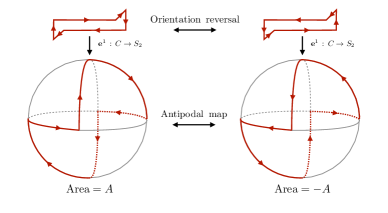
Figure 3: Schematics of two paths, related by reversal of orientation, and their mappings on the sphere. The implementation of orientation reversal on the sphere is realized by an antipodal map: $\mathcal{A}(\bm{e}^{1})=-\bm{e}^{1}$. The enclosed signed areas of the paths are $2\pi$ and $-2\pi$.

Let us look more carefully at the effective action for the relativistic composite boson, Eq. (50), and do the following reasoning. Remember that $\Omega_{flat}$ is the signed area enclosed by a given worldline $C$ on the sphere $S_{2}$, defined by $\bm{e}^{1}:C\rightarrow S_{2}$. Now suppose that we want to reverse the orientation of $C$. We can do it by implementing an antipodal map on the sphere, this is, under orientation reversal each point of a given path $C$ on $S_{2}$ is mapped to its antipodal point. This is easy to see by noting that reversing orientation is basically flipping the sign of the unit tangent vector at each point on $C$. Thus, any path on $S_{2}$ is mapped to its antipodal path, see figure 3. If the signed area enclosed by a given path on $S_{2}$ is $A$, then the area of the antipodal path is $-A$. This means that under orientation reversal, $\Omega_{flat}\rightarrow-\Omega_{flat}$ and $\exp(i\Omega_{flat}/2)$ is complex conjugated. Having this in mind, we perform the following trivial manipulation

$$e^{\frac{i}{2}\Omega_{flat}}\,e^{i\int_{0}^{t}ds\,\big{(}A_{\mu}\dot{X}^{\mu}-\frac{1}{4}e^{1a}\epsilon_{abc}\,\tensor{\omega}{{}_{\mu}^{b}{}^{c}}\dot{X}^{\mu}\big{)}}= \,e^{i\int_{0}^{t}ds\,A_{\mu}\dot{X}^{\mu}}\cos\Big{(}\frac{\Omega_{flat}}{2}-\int_{0}^{t}ds\,\frac{1}{4}e^{1a}\epsilon_{abc}\,\tensor{\omega}{{}_{\mu}^{b}{}^{c}}\dot{X}^{\mu}\Big{)}$$

$$+\Big{(}i\cos\int_{0}^{t}ds\,A_{\mu}\dot{X}^{\mu}-\sin \int_{0}^{t}ds\,A_{\mu}\dot{X}^{\mu}\Big{)}\sin\frac{\Omega_{flat}}{2}\,\cos\Big{(}\frac{1}{4}\int_{0}^{t}ds\,e^{1a}\epsilon_{abc}\,\tensor{\omega}{{}_{\mu}^{b}{}^{c}}\dot{X}^{\mu}\Big{)}$$

$$-\Big{(}i\cos\int_{0}^{t}ds\,A_{\mu}\dot{X}^{\mu}-\sin \int_{0}^{t}ds\,A_{\mu}\dot{X}^{\mu}\Big{)}\cos\frac{\Omega_{flat}}{2}\,\sin\Big{(}\frac{1}{4}\int_{0}^{t}ds\,e^{1a}\epsilon_{abc}\,\tensor{\omega}{{}_{\mu}^{b}{}^{c}}\dot{X}^{\mu}\Big{)}.$$ (65)

Contrary to $\Omega_{flat}$ and $\int_{0}^{t}ds\,A_{\mu}\dot{X}^{\mu}$, the spin connection term remains invariant under reversal of orientation. This is of no surprise, since reversing orientation of the worldlines can be seen as a charge conjugation operation. Applying Eq. (65) to the effective action (50), and after integrating over all worldline configurations, which include both forward and backward orientations for each path, odd terms under orientation reversal vanish and the r.h.s. of Eq.(65) becomes

$$e^{i\int_{0}^{t}ds\,A_{\mu}\dot{X}^{\mu}}\cos\Big{(}\frac{\Omega_{flat}}{2}-\int_{0}^{t}ds\,\frac{1}{4}e^{1a}\epsilon_{abc}\,\tensor{\omega}{{}_{\mu}^{b}{}^{c}}\dot{X}^{\mu}\Big{)}-\sin\int_{0}^{t}ds\,A_{\mu}\dot{X}^{\mu}\,\sin\frac{\Omega_{flat}}{2}$$

$$\times\cos\Big{(}\frac{1}{4}\int_{0}^{t}ds\,e^{1a}\epsilon_{abc}\,\tensor{\omega}{{}_{\mu}^{b}{}^{c}}\dot{X}^{\mu}\Big{)}-i\cos\int_{0}^{t}ds\,A_{\mu}\dot{X}^{\mu}\,\cos\frac{\Omega_{flat}}{2}\,\sin\Big{(}\frac{1}{4}\int_{0}^{t}ds\,e^{1a}\epsilon_{abc}\,\tensor{\omega}{{}_{\mu}^{b}{}^{c}}\dot{X}^{\mu}\Big{)}.$$ (66)

The effective action must preserve charge conjugation symmetry, which means that odd terms in $A_{\mu}$ should vanish (by Furry’s theorem). Then the second term in Eq. (66) vanishes. The third term makes up the imaginary part of the bosonic effective action. It contains only odd powers of the spin connection, and because there is no locally Lorentz invariant term that can be constructed with odd powers of $\omega_{\mu}$ alone, it should vanish as well. We are thus left with

$$e^{\frac{i}{2}\Omega_{flat}}\,e^{i\int_{0}^{t}ds\,\big{(}A_{\mu}\dot{X}^{\mu}-\frac{1}{4}e^{1a}\epsilon_{abc}\,\tensor{\omega}{{}_{\mu}^{b}{}^{c}}\dot{X}^{\mu}\big{)}}=e^{i\int_{0}^{t}ds\,A_{\mu}\dot{X}^{\mu}}\cos\Big{(}\frac{\Omega_{flat}}{2}-\int_{0}^{t}ds\,\frac{1}{4}e^{1a}\epsilon_{abc}\,\tensor{\omega}{{}_{\mu}^{b}{}^{c}}\dot{X}^{\mu}\Big{)}.$$ (67)

4.1 Duality as a mapping between phases

In order to be able to compare bosonic and fermionic effective actions we note that the $|\phi|^{4}$ interaction is relevant, which means that its strength grows as we run to the IR. For massive excitations, we can assume our energy scale to be sufficiently far away from the IR, such that treating the interactions perturbatively seems reasonable. Doing so and inserting Eq. (67) in (50) we obtain, for the effective action for the relativistic composite boson

$$Z_{scalar+flux}=e^{-\Gamma_{scalar+flux}}$$

$$\Gamma_{scalar+flux}=\int_{\epsilon}^{\infty}dt\,t^{-1}\,\int DX^{\mu}\,e^{-\int_{0}^{t}ds\big{(}\frac{1}{4}\dot{X}^{2}-iA_{\mu}\dot{X}^{\mu}+\frac{R}{4}+m^{2}\big{)}}$$

$$\times\cos\Big{[}-\frac{1}{4}\int_{0}^{t}ds\,e^{1a}\epsilon_{abc}\tensor{\omega}{{}_{\mu}^{b}{}^{c}}\dot{X}^{\mu}+\frac{\Omega_{flat}}{2}\Big{]}+iCS_{g}+\mathcal{O}(\lambda),$$ (68)

where $\mathcal{O}(\lambda)$ includes (short-range) interacting terms at all non-trivial orders in $\lambda$. By comparison with the real part of the fermion effective action, Eq. (64), we see that the Pauli term in the spin factor (inside the cosine), proportional to $F^{*}_{\mu}(A)$, is missing in Eq. (68). Such a term is a consequence of the spin angular momentum of the Dirac spinor, and contributes to the even part of the vacuum polarization in the fermionic side (and in general to the N-photon amplitudes). While it can not be reproduced in the bosonic side, $F^{*}_{\mu}(A)$ is an irrelevant operator, which means that its value decreases towards the IR, vanishing at the IR fixed point. We can write

$$\mathcal{R}(\Gamma_{scalar+flux})\approx\mathcal{R}(\Gamma_{f})+\mathcal{O}(\lambda),$$ (69)

where $\approx$ means that the equality is only valid up to irrelevant terms of the order $\mathcal{O}\big{(}F^{*}_{\mu}(A)\big{)}$.

4.1.1 Duality as a mapping between topological phases

Turning our attention to the map between imaginary parts of effective actions, let us first pick a specific regularization for the parity anomaly of the fermion, say

$$\mathcal{I}(\Gamma_{f})=-\big{(}\mathrm{sign}(m)-1\big{)}\Big{(}\frac{CS_{A}}{2}+CS_{g}\Big{)}.$$ (70)

We see that, if the mass is negative, Eq. (70) does not match the imaginary part of the $\Gamma_{scalar+flux}\,$. On the one hand, the electromagnetic CS term is missing in $\Gamma_{scalar+flux}\,$, so to obtain an equality between imaginary parts of effective actions we need to add a counterterm of the form $iCS_{A}$ to the bosonic side. On the other hand, there is a mismatch between the gravitational contributions. The framing anomaly as in Eq. (49) gives a contribution $iCS_{g}$ to $\Gamma_{scalar+flux}\,$, whereas the fermionic gravitational contribution in (70) is twice as big, $i2CS_{g}$. We need to add a gravitational CS term $iCS_{g}$, which we can think of as an alternative regularization of the framing anomaly, so that the partition function of the free CS theory takes the form $Z_{CS}=e^{-i2CS_{g}}$. This choice of regularization for the framing anomaly has been recently used in this context [35], in order to obtain the correct boson-fermion mapping. Adding the above two terms we get

$$\Gamma_{scalar+flux}+iCS_{A}+iCS_{g}\approx\Gamma_{f}+\mathcal{O}(\lambda)$$ (71)

In Lagrangian form this translates to

$$\big{|}D_{\mu}(a)\phi\big{|}^{2}-(\frac{R}{4}+m^{2})|\phi|^{2}-\lambda|\phi|^{4}-\frac{1}{4e}F^{2}(a)+CS_{a}-CS_{g}+\frac{1}{2\pi}\epsilon^{\mu\rho\nu}a_{\mu}\partial_{\rho}A_{\nu}$$

$$\ext@arrow 3359\leftrightarrowfill@{}{e\rightarrow\infty}$$

$$\bar{\Psi}\big{(}i\not{D}(\omega,A)-m\big{)}\Psi+\,.\,.\,.$$ (72)

where we have done the shift $a_{\mu}\rightarrow a_{\mu}-A_{\mu}$, and where $m$ is negative: $m=-|m|$. By $\,.\,.\,.$ we denote short-range fermionic interactions, that account for the short-range interactions, $\mathcal{O}(\lambda)$, in the bosonic side. It’s important to note that the correspondence in Eq. (72) is only valid up to induced irrelevant terms of the order $\mathcal{O}\big{(}F^{*}_{\mu}(A)\big{)}$ in the fermionic effective action.

Eq. (72) is a mapping between theories in a topological phase (usually referred to as the Chern insulator in condensed matter physics). The bosonic side flows, when the mass is taken to vanish, towards the IR Wilson-Fisher-CS fixed point, which is a strongly short-range interacting theory of massless bosons coupled to a CS field. So, even if the bare value of the quartic coupling is not tuned to the Wilson-Fisher fixed point, the RG flows in the IR to this fixed point. In other words, the fixed point theory and the bare theory differ in irrelevant operators that, at most, yield corrections to scaling.

Regarding the fermionic side, in the free Dirac theory the short-range four-fermion interactions (denoted by $.\,.\,.$) are irrelevant, and consequently vanish in the IR. Thus, in the IR we flow to the free massless Dirac fermion fixed point. The same happens with the irrelevant terms in $F^{*}_{\mu}(A)$ in the fermionic effective action that spoil the mapping (72). Therefore, our results are consistent with the conjectured exact duality between a Wilson-Fisher-CS complex scalar and a free massless Dirac fermion at the IR fixed point [36, 35].

It is important to emphasize that in a construction of both theories along the lines used in this work (and, in fact, in any local construction) the resulting theory is not automatically a CFT since, as we showed here, there are always irrelevant operators. Thus, the duality mappings are asymptotic statements of both theories deep in the IR. That this is the case is an assumption of the CFT constructions of the dualities.

4.1.2 Duality as a mapping between trivial phases

Now we can think of flipping the sign of the fermion mass, this time to be positive. In this scenario the imaginary part of the fermionic effective action vanishes, and the fermionic side is now in a topologically trivial phase. This situation is understood to correspond to the U(1) symmetry broken (Higgs) phase of the composite boson [36, 35]. This has very recently been proven, in the context of loop models, by Goldman and one of us [53] by making use of the particle-vortex duality, and writing the loop model partition function in the broken phase as one describing the symmetric phase of dual variables $\tilde{\phi}$. We are going to use the same procedure here in order to obtain the boson-fermion duality in the trivial phase. First, we invoke the mentioned particle-vortex mapping

$$\big{|}D_{\mu}(B)\phi\big{|}^{2}+m^{2}|\phi|^{2}-\lambda|\phi|^{4}\longleftrightarrow\big{|}D_{\mu}(\tilde{b})\tilde{\phi}\big{|}^{2}-m^{\prime 2}|\tilde{\phi}|^{2}-\lambda^{\prime}|\tilde{\phi}|^{4}+\frac{1}{2\pi}\epsilon^{\mu\rho\nu}\tilde{b}_{\mu}\partial_{\rho}B_{\nu}.$$ (73)

The map identifies the Higgs phase of $\phi$ variables (note the positive sign in front of $m^{2}$) with the symmetric phase of $\tilde{\phi}$ variables. We can add now $CS_{B}+\epsilon^{\mu\rho\nu}B_{\mu}\partial_{\rho}A_{\nu}/2\pi$ to both sides, and promote $B_{\mu}$ to a dynamical field $b_{\mu}$. After integrating out $b_{\mu}$ on the r.h.s. we obtain

$$\big{|}D_{\mu}(b)\phi\big{|}^{2}+m^{2}|\phi|^{2}-\lambda|\phi|^{4}+CS_{b}+\frac{1}{2\pi}\epsilon^{\mu\rho\nu}b_{\mu}\partial_{\rho}A_{\nu}$$

$$\longleftrightarrow$$

$$\big{|}D_{\mu}(\tilde{b})\tilde{\phi}\big{|}^{2}-m^{\prime 2}|\tilde{\phi}|^{2}-\lambda^{\prime}|\tilde{\phi}|^{4}-CS_{\tilde{b}}-CS_{A}-\frac{1}{2\pi}\epsilon^{\mu\rho\nu}\tilde{b}_{\mu}\partial_{\rho}A_{\nu}$$ (74)

We can make use of this duality and write the composite boson, appearing in the bosonic side of duality (72), in its Higgs phase in terms of the $\tilde{\phi}$ field in its symmetric phase. We get

$$\big{|}D_{\mu}(\tilde{a})\tilde{\phi}\big{|}^{2}-(\frac{R}{4}+m^{2})|\tilde{\phi}|^{2}-\lambda|\tilde{\phi}|^{4}-\frac{1}{4e}F^{2}(\tilde{a})-CS_{\tilde{a}}-CS_{A}-CS_{g}-\frac{1}{2\pi}\epsilon^{\mu\rho\nu}\tilde{a}_{\mu}\partial_{\rho}A_{\nu}$$ (75)

It is clear that the real part of the effective action arising from (75) is basically that of the $\phi$ fields in the symmetric phase, $\mathcal{R}(\Gamma_{scalar+flux})$, as given by Eq. (68). On the other hand, the sign flip in the CS term for the dynamical gauge field $\tilde{a}_{\mu}$ gives a framing anomaly with gravitational CS term of opposite sign, $CS_{g}$, canceling the background contribution $-CS_{g}$. A similar thing happens for $A_{\mu}$: doing the shift $\tilde{a}_{\mu}\rightarrow\tilde{a}_{\mu}+A_{\mu}$, the resulting CS term, $CS_{A}$, is canceled by the extra term $-CS_{A}$. This means that the effective action arising from Eq. (75) is real, and is therefore equal to the effective action of a Dirac fermion of positive mass (with the chosen specific regularization of the parity anomaly). We have then proven that the composite boson $\phi$ in its Higgs phase is dual to a Dirac fermion of positive mass.

5 Concluding remarks and outlook

We have revisited Polyakov’s duality between a massive relativistic composite boson and a massive Dirac fermion, in the presence of background curvature and electromagnetic fields. The duality holds in curved space-time, as long as a non-minimal coupling to curvature is included in the bosonic side, but holds only up to an irrelevant operator when fermions and bosons are coupled to a background gauge field. This is rooted to the obtained spin factor for the Dirac fermion (see Eq. (64)), which has both electromagnetic and gravitational contributions. While the gravitational contribution is provided naturally, in the bosonic side, by the extension of the Wilson loop to curved backgrounds, the electromagnetic contribution (Pauli term) is a consequence of the spin angular momentum of the spinor and can not be reproduced in the bosonic side.

The addition of background fields to Polyakov’s construction has to be treated with care, as now the parity and framing anomaly of fermions and CS fields come in to fore. The mapping between partition functions can only be defined after proper regularizations for the anomalies have been specified. For the parity anomaly of the fermion, gauge invariance must be imposed, and a regularization dependent time-reversal breaking CS term appears in the effective action. Further fixing the sign of the CS term completely removes the ambiguity on the regularization of the parity anomaly. In regards to the framing anomaly, we included a Maxwell term, $F^{2}/e^{2}$, for the CS gauge field. Its purpose is to act as a regulator that forces the CS theory to be quantized in a non-topological, but frame invariant, way. The duality is then defined after removing the regulator, i.e. at infinite coupling $e\rightarrow\infty$. A metric dependent regularization of the CS theory is necessary in two levels: first, it is needed to obtain the spin factor from the Wilson loop, responsible of transmuting a boson into a fermion, and second, it is necessary to obtain the gravitational CS term from the framing anomaly of the pure CS theory, such that the imaginary parts (in Euclidean signature) of the effective actions at both sides of the duality match.

The inclusion of $|\phi|^{4}$ interactions in the bosonic side is of crucial importance to resolve another subtlety of Polyakov’s mapping. The machinery behind the boson-fermion duality relies on a topological property of Wilson loops in the CS theory. Basically, closed worldline configurations are classified in terms of the Gauss’s linking number, such that interactions between worldlines vanish for specific values of the statistical angle: $\delta=n\pi$, with $n\in\mathbb{Z}$ (in our case, $\delta=\pi$). The subtlety lies in the fact that, in the absence of interactions between bosons, worldlines could intersect, in which case the linking number would not be well defined. Other way of seeing this is that if intersections are not avoided, linked worldlines and knots could be unlinked and unknotted, and their topological properties would not be preserved. The $|\phi|^{4}$ term solves this issue, providing short-ranged interactions between worldlines that suppress intersecting worldline configurations. The short-range bosonic interactions map to short-range interactions in the fermionic side, with the crucial difference that, unlike the $|\phi|^{4}$ interactions, which are relevant, short-range fermionic interactions are irrelevant. Thus, when the mass is set to zero, the fermionic side flows to a non-interacting Dirac fermion at the IR fixed point, while the bosonic side flows to a (strongly interacting) Wilson-Fisher-CS complex scalar.

The massive fermionic and bosonic theories at both sides of the duality can be either in a trivial or a topological phase. If the fermion is in the topological phase, it maps to a composite boson in its $U(1)$ symmetric phase, whereas if it is in the trivial phase, the mapping is to a composite boson in its $U(1)$ symmetry broken (Higgs) phase. To prove this last case, instead of working directly in the Higgs phase we followed Ref. [53] and made use of the particle-vortex duality, writing the Higgs phase of the $\phi$ field as the $U(1)$ symmetric phase of a dual field $\tilde{\phi}$. Once working in the dual picture, the proof of the duality is analogous to that for the $\phi$ field in its symmetric phase.

Our work opens the path for computing gravitational and geometric responses of relativistic composite bosons. Some responses in condensed matter systems, like the Hall viscosity, can acquire torsional contributions. In solids, torsion can arise naturally in the form of dislocations. Henceforth, one interesting extension of the present work is to allow for a background with torsion. Another future appealing direction is to extend the formalism presented here to prove dualities involving non-Abelian CS-matter theories. Specifically, a recent conjectured duality between a Majorana fermion and a $SO(N)$ vector boson coupled to a $SO(N)$ CS gauge field [41, 42] could be of relevance in a condensed matter context.

Appendix A Effective action manipulations

A.1 Effective action for the scalar field as a worldline path integral

To write the effective action, Eq. (12), as an integral over worldlines, we make use of the following identities

$$\partial_{s}H^{-s}|_{s\rightarrow 0}=-\ln H,$$ (76)

$$H^{-s}=\frac{\int^{\infty}_{0}dt\,t^{s-1}e^{-Ht}}{\int_{0}^{\infty}dt\,t^{s-1}e^{-t}}=\frac{1}{\Gamma(s)}\int^{\infty}_{0}dt\,t^{s-1}e^{-Ht},$$ (77)

Using $\Gamma^{-1}(s)=s+\mathcal{O}(s^{2})$, we can write

$$-\Gamma^{\prime}=-\mathrm{tr}\ln H=\mathrm{tr}\int_{\epsilon}^{\infty}dt\,t^{-1}\,e^{-tH},$$ (78)

with

$$H=-\frac{1}{\sqrt{g}}D_{\mu}(a,A)\sqrt{g}\,g^{\mu\nu}D_{\nu}(a,A)+\frac{R}{4}+m^{2}+2i\sqrt{\lambda}\,\sigma,$$ (79)

and where we introduced a UV cut-off $\epsilon$. Now let us do time slicing and discretize the action as a sum over N random paths of length $\Delta t$

$$-\Gamma=\int_{\epsilon}^{\infty}dt\,t^{-1}\int\prod_{i=1}^{N}d^{3}X_{i}\,\delta(X_{N}-X_{0})\langle X_{i}|e^{-\Delta t\,H}|X_{i-1}\rangle,$$ (80)

where $\Delta t=t/N$ and

$$\langle X_{i}|e^{-\Delta t\,H}|X_{i-1}\rangle$$

$$=\int\frac{d^{3}p}{(2\pi)^{3}}\exp\Big{[}-\Delta t\Big{(}ip_{\mu}\Delta X^{\mu}_{i}+\big{(}p_{\mu}+a_{\mu}+A_{\mu}\big{)}\big{(}p^{\mu}+a^{\mu}+A^{\mu}\big{)}+\frac{R}{4}+m^{2}+2i\sqrt{\lambda}\,\sigma\Big{)}\Big{]}$$

$$=\sqrt{g}\,\left(\frac{1}{4\pi\Delta t}\right)^{3/2}\exp\Big{[}-\Delta t\Big{(}\frac{1}{4}g_{\mu\nu}\Delta X^{\mu}_{i}\Delta X^{\nu}_{i}-i(a_{\mu}+A_{\mu})\Delta X^{\mu}_{i}+\frac{R}{4}+m^{2}+2i\sqrt{\lambda}\,\sigma\Big{)}\Big{]},$$ (81)

with $\Delta X^{\mu}_{i}=(X^{\mu}_{i}-X^{\mu}_{i-1})/\Delta t$. Now we take the limit $\Delta t\rightarrow 0$ and obtain

$$-\Gamma=\int_{\epsilon}^{\infty}dt\,t^{-1}\,DX^{\mu}\,\exp\left[-\int_{0}^{t}ds\Big{(}\frac{1}{4}\dot{X}^{2}-i(a_{\mu}+A_{\mu})\dot{X}^{\mu}+\frac{R}{4}+m^{2}+2i\sqrt{\lambda}\,\sigma\Big{)}\right],$$ (82)

with $X^{\mu}(t)=X^{\mu}(0)$ and $\dot{X}^{2}=g_{\mu\nu}\dot{X}^{\mu}\dot{X}^{\nu}$. The integration measure is defined as

$$\int DX^{\mu}=\lim_{\Delta t\rightarrow 0}\int\prod_{i=1}^{N}\left(\frac{1}{4\pi\Delta t}\right)^{3/2}\sqrt{g_{i}}\,d^{3}X_{i}.$$ (83)

It fulfills the normalization condition

$$\int\prod_{i=1}^{N}\left(\frac{1}{4\pi\Delta t}\right)^{3/2}\sqrt{g_{i}}\,d^{3}X_{i}\,e^{-\Delta t\,g_{i,\mu\nu}\Delta X^{\mu}_{i}\Delta X^{\nu}_{i}/4}=1.$$ (84)

A.2 Effective action as a regularized path integral over the unit tangent vector

Although not relevant for the main results of this work, we would like to show how one can further manipulate the worldline effective actions Eq.(50) and (64), and write them as a regularized path integral over the unit vector tangent to the worldlines, $e^{1\mu}$. We start from the following general effective action

$$-\Gamma=-\int_{\epsilon}^{\infty}dt\,t^{-1}\,DX^{\mu}\,\exp\left[-\int_{0}^{t}ds\Big{(}\frac{1}{4}\dot{X}^{2}-iB_{\mu}\dot{X}^{\mu}+M^{2}\Big{)}\right]\,e^{i\Omega_{flat}/2},$$ (85)

where $B_{\mu}$ and $M$ are generic vector and scalar fields, respectively. Let us regularize it by doing time slicing over N random paths of length $\tilde{\epsilon}=\Delta t$, as done in appendix A.1

$$-\Gamma=-\int_{\epsilon}^{\infty}dt\,t^{-1}\left(\frac{1}{4\pi\tilde{\epsilon}}\right)^{3N/2}\int\Bigg{(}\prod_{i=1}^{N}\sqrt{g_{i}}\,d^{3}X_{i}\,\delta(X_{N}-X_{0})$$

$$\times\,\exp\Big{[}-\tilde{\epsilon}\Big{(}\frac{1}{4}\Delta X^{2}_{i}-iB_{\mu}\Delta X^{\mu}_{i}+M^{2}\Big{)}\Big{]}\Bigg{)}\,e^{i\Omega_{flat}/2},$$ (86)

where $\tilde{\epsilon}$ acts as an UV cut-off. Now one can do a change of integration variables $v^{\mu}_{i}=\Delta X^{\mu}_{i}$ and write the delta function as

$$\delta(X_{N}-X_{0})=\delta(\tilde{\epsilon}\sum_{i=1}^{N}v_{i})=\prod_{i=1}^{N}\int\frac{d^{3}k}{(2\pi)^{3}}\,e^{\tilde{\epsilon}ik_{\mu}v^{\mu}_{i}},$$ (87)

so the effective action can be written as

$$-\Gamma=-\int_{\epsilon}^{\infty}dt\,t^{-1}\left(\frac{\tilde{\epsilon}}{4\pi}\right)^{3N/2}\int\frac{d^{3}k}{(2\pi)^{3}}\int\Bigg{(}\prod_{i=1}^{N}\sqrt{g_{i}}\,\hat{v}^{\mu}_{i}\,dv_{i}\,v_{i}^{2}$$

$$\times\,\exp\Big{[}-\tilde{\epsilon}\Big{(}\frac{1}{4}v_{i}^{2}-iv_{i}(k_{\mu}+B_{\mu})\hat{v}^{\mu}_{i}+M^{2}\Big{)}\Big{]}\Bigg{)}\,e^{i\Omega_{flat}/2},$$ (88)

where we have done $\int dv^{\mu}_{i}=\int d\hat{v}^{\mu}_{i}\,dv_{i}\,v_{i}^{2}$, and we should remember that $\Omega_{flat}$ does not depend on $v_{i}$, but only on the unit vector $\hat{v}^{\mu}_{i}$. Integrating over the radial coordinates $v_{i}$ and doing the change of variables $L=4t/\sqrt{\pi\tilde{\epsilon}}$ [22]

$$-\Gamma=-\int_{\epsilon^{\prime}}^{\infty}dL\,L^{-1}\int\frac{d^{3}k}{(2\pi)^{3}}\int\Bigg{(}\prod_{i=1}^{N}\sqrt{g_{i}}\,\frac{d\hat{v}^{\mu}_{i}}{4\pi}\,e^{-\frac{\sqrt{\pi\tilde{\epsilon}}}{4}M^{2}\Delta L}$$

$$\times\,e^{\Delta L\,i(k_{\mu}+B_{\mu})\hat{v}^{\mu}_{i}}\,e^{i\mathcal{O}(\sqrt{\tilde{\epsilon}})}\Bigg{)}\,e^{i\Omega_{flat}/2},$$ (89)

where $\Delta L=L/N$, and

$$\mathcal{O}(\sqrt{\tilde{\epsilon}})\sim\sqrt{\tilde{\epsilon}}\,\Delta L\Big{(}(k_{\mu}+B_{\mu})\hat{v}^{\mu}_{i}\Big{)}^{2}+\mathcal{O}(\tilde{\epsilon}^{3/2})$$ (90)

$$\epsilon^{\prime}=\frac{4}{\sqrt{\pi\tilde{\epsilon}}}\epsilon.$$ (91)

Taking the continuum limit $\Delta L\rightarrow 0$ and renaming $e^{1\mu}\equiv\hat{v}^{\mu}$

$$-\Gamma=-\int\frac{d^{3}k}{(2\pi)^{3}}\int_{\epsilon^{\prime}}^{\infty}\frac{dL}{L}\,e^{-\int_{0}^{L}ds\frac{\sqrt{\pi\tilde{\epsilon}}}{4}M^{2}}\int De^{1\mu}\,e^{i\int_{0}^{L}ds(k_{\mu}+B_{\mu})e^{1\mu}}\,e^{i\Omega_{flat}/2}\,e^{i\mathcal{O}(\sqrt{\tilde{\epsilon}})},$$ (92)

$$\mathcal{O}(\sqrt{\tilde{\epsilon}})\sim\sqrt{\tilde{\epsilon}}\int_{0}^{L}ds\Big{(}(k_{\mu}+B_{\mu})e^{1\mu}\Big{)}^{2}+\mathcal{O}(\tilde{\epsilon}^{3/2})$$ (93)

with $De^{1\mu}=\delta(e^{1}-1)de^{1\mu}/4\pi=\prod_{i=1}^{N}\delta(e^{1}_{i}-1)\sqrt{g_{i}}\,de^{1\mu}_{i}/4\pi$.

Using the previous result, we can write the effective actions for the composite boson and the two time-reversal partner Dirac fermions, Eqs. (50) and (64), as

$$\Gamma_{scalar+flux}=\int\frac{d^{3}k}{(2\pi)^{3}}\int_{\epsilon^{\prime}}^{\infty}dL\,L^{-1}\,e^{-\int_{0}^{L}ds\,\frac{\sqrt{\pi\tilde{\epsilon}}}{4}\,\big{(}\frac{R}{4}+m^{2}+2i\sqrt{\lambda}\,\sigma\big{)}}$$

$$\times\int De^{1\mu}\,\,e^{i\int_{0}^{L}ds\big{(}k_{\mu}+A_{\mu}-\frac{1}{4}e^{1a}\epsilon_{abc}\,\tensor{\omega}{{}_{\mu}^{b}{}^{c}}\big{)}e^{1\mu}}e^{\frac{i}{2}\Omega_{flat}}e^{i\mathcal{O}(\sqrt{\tilde{\epsilon}})}\,+iCS_{g},$$ (94)

with

$$\mathcal{O}\big{(}\sqrt{\tilde{\epsilon}}\big{)}\sim\sqrt{\tilde{\epsilon}}\int_{0}^{L}ds\,\Big{[}\big{(}k_{\mu}+A_{\mu}-\frac{1}{4}e^{1a}\epsilon_{abc}\,\tensor{\omega}{{}_{\mu}^{b}{}^{c}}\big{)}e^{1\mu}\Big{]}^{2}+\mathcal{O}\big{(}\tilde{\epsilon}^{3/2}\big{)},$$ (95)

and

$$2\mathcal{R}(\Gamma_{f})=\int\frac{d^{3}k}{(2\pi)^{3}}\int_{\epsilon^{\prime}}^{\infty}dL\,L^{-1}\,e^{-\int_{0}^{L}ds\,\frac{\sqrt{\pi\tilde{\epsilon}}}{4}\,\big{(}\frac{R}{4}+m^{2}+2i\sqrt{\lambda}\,\sigma\big{)}}$$

$$\times\int De^{1\mu}\,\sum_{\alpha=\pm 1}\,e^{i\int_{0}^{L}ds\,(k_{\mu}+A_{\mu}+\alpha iF^{*}_{\mu}(A)-\alpha\frac{1}{4}e^{1a}\epsilon_{abc}\,\tensor{\omega}{{}_{\mu}^{b}{}^{c}})e^{1\mu}}\,e^{\alpha\frac{i}{2}\Omega_{flat}}\,e^{i\mathcal{O}_{\alpha}\big{(}\sqrt{\tilde{\epsilon}}\big{)}},$$ (96)

with

$$\mathcal{O}_{\alpha}\big{(}\sqrt{\tilde{\epsilon}}\big{)}\sim\sqrt{\tilde{\epsilon}}\int_{0}^{L}ds\,\Big{[}\big{(}k_{\mu}+A_{\mu}-\alpha\frac{1}{4}e^{1a}\epsilon_{abc}\,\tensor{\omega}{{}_{\mu}^{b}{}^{c}}\big{)}e^{1\mu}\Big{]}^{2}+\mathcal{O}\big{(}\tilde{\epsilon}^{3/2}\big{)}.$$ (97)

Appendix B The twist as a Berry phase

We follow [19] and show that the twist,

$$T=\frac{1}{2\pi}\int_{0}^{t}ds\,\bm{e}^{1}\cdot(\bm{e}^{2}\times\dot{\bm{e}}^{2}),$$ (98)

can be written as a Berry phase [19, 112, 113], which itself can be written as a Wess-Zumino-Witten term. Defining $\omega=\omega_{1}\bm{e}^{1}+\omega_{i}\bm{e}^{i}$ as the rate of rotation of the frame along C: $\dot{\bm{e}}^{1}=\omega\times\bm{e}^{1}$, $\dot{\bm{e}}^{i}=\omega\times\bm{e}^{i}$ ($i=1,2$), we can rewrite T as

$$T=\frac{1}{2\pi}\int_{0}^{t}\,\omega_{1}ds,$$ (99)

with $\omega_{1}=\dot{\bm{e}}^{2}\times\bm{e}^{3}$.

Let us now introduce two $CP^{1}$ fields z and w which satisfy

$$z^{\dagger}\bm{\sigma}z=\bm{e}^{1},\quad w^{\dagger}\bm{\sigma}w=-\bm{e}^{1},$$ (100)

so that $w_{1}=-z_{2}^{*}$, $w_{2}=z_{1}^{*}$. Next we define the complex vector $\bm{v}=z^{\dagger}\bm{\sigma}w$ which, using Eq. (100), is easy to show to be orthogonal to $\bm{e}^{1}$. By further using the properties of the sigma matrices, one can prove that $\bm{v}$ is equal to the combination $\bm{e}^{2}-i\bm{e}^{3}$ up to a phase [19]

$$\bm{v}=e^{i\alpha}(\bm{e}^{2}-i\bm{e}^{3}),$$ (101)

with $\alpha(t)=\alpha(0)+2\pi\nu$, where $\nu\in\mathbb{Z}$ is the winding number. Recalling the definition $\omega_{1}=\dot{\bm{e}}^{2}\times\bm{e}^{3}$, one can show that

$$\bm{v}\cdot\dot{\bm{v}}^{*}=4z^{\dagger}\cdot\dot{z}=-2i(\dot{\alpha}+\omega_{1}).$$ (102)

We get

$$T=\frac{1}{2\pi}\int_{0}^{t}\omega_{1}\,ds=\frac{i}{\pi}\int_{0}^{t}\,z^{\dagger}\cdot\dot{z}-\frac{1}{2\pi}\int_{0}^{t}\dot{\alpha}\,ds=-\frac{1}{\pi}\int_{0}^{t}A(s)\,ds-\nu,$$ (103)

where we have introduced the Berry connection $A=-iz^{\dagger}\cdot\dot{z}$, so that $T$ is written as a Berry phase plus a winding number. Let us study the dependence of the twist on the framing, by performing the rotation

$$\tilde{\bm{e}}^{2}=\cos\varphi\,\bm{e}^{2}+\sin\varphi\,\bm{e}^{3},\quad\quad\tilde{\bm{e}}^{3}=-\sin\varphi\,\bm{e}^{2}+\cos\varphi\,\bm{e}^{3},$$ (104)

where periodicity demands $\varphi(t)=\varphi(0)+2\pi m$, with $m\in\mathbb{Z}$. This shifts the phase in Eq. (101): $\tilde{\alpha}=\alpha+\varphi$. Therefore, the twist transforms as

$$\tilde{T}=T-m,$$ (105)

which confirms its frame dependence.

Finally, as we are dealing with closed paths, the Berry phase is just the enclosed flux of the Berry curvature, which can be defined by continuing $s\in C$ to $u\in S$, where S is the surface enclosed by C

$$\frac{1}{\pi}\int_{0}^{t}A(s)\,ds=\frac{1}{\pi}\int_{S}d^{2}u(\partial_{u_{1}}A_{2}-\partial_{u_{2}}A_{1})=\frac{1}{2\pi}\int_{0}^{1}d\rho\int_{0}^{t}ds\,\bm{e}^{1}\cdot(\partial_{\rho}\bm{e}^{1}\times\partial_{s}\bm{e}^{1}).$$ (106)

In the last equality the surface $S$ is parametrized by $s\in[0,t]$ and $\rho\in[0,1]$, and $\bm{e}^{1}$ is extended to $\bm{e}^{1}(t,\rho)$ in such a way that $\bm{e}^{1}(t,0)=\bm{e}_{0}$ and $\bm{e}^{1}(t,1)=\bm{e}^{1}(t)$, with $\bm{e}_{0}$ some constant vector. The last term is precisely the Wess-Zumino-Witten term [114, 115], and is equal to the signed area enclosed by the path C on the sphere $S_{2}$, defined by $\bm{e}^{1}:C\rightarrow S_{2}$. Then, the gauge field $A(s)$ can be interpreted as that of a monopole at the center of the sphere, so that the signed area is proportional to the magnetic flux enclosed.

Appendix C The spin factor as a path integral over anticommuting fields

Let us show how, in the absence of curvature, the spin factor can be defined as a path integral over one dimensional fermions, and how one can then extend this definition to curved space. We start with the following path integral over anticommuting fields $\psi^{a}$ [111, 121]

$$\int D\psi^{a}D\chi\,e^{\int_{0}^{t}ds\,(\frac{1}{4}\psi_{a}\dot{\psi}_{a}+\chi e^{1}_{a}\psi_{a})},$$ (107)

where $\chi$ acts as a Lagrange multiplier imposing transversality of the fields $\psi^{a}$, as can be seeing by integrating it out

$$\int D\psi^{a}\,\delta(\psi^{a}e^{1}_{a})\,e^{\frac{1}{4}\int_{0}^{t}ds\,\psi_{a}\dot{\psi}_{a}}.$$ (108)

Doing the change of variables

$$\psi_{a}=2e^{1}_{a}\phi^{1}+2e^{i}_{a}\phi_{i},$$ (109)

with $i=2,3$, we get

$$\int D\phi^{1}D\phi^{i}\,\delta(2\phi^{1})\,e^{\int_{0}^{t}ds\,(\phi_{i}\dot{\phi}_{i}+\omega_{1}\epsilon_{ij}\phi_{i}\phi_{j})},$$ (110)

where $\omega_{1}$ is defined in appendix B. Taking into account that the correlator $\langle\phi_{i}(s)\phi_{j}(s^{\prime})\rangle$ with respect to the action $\int_{0}^{t}ds\,\phi_{i}\dot{\phi}_{i}$ is $\delta_{ij}\,sgn(s-s^{\prime})$, it is not difficult to prove that [111, 121]

$$\int D\phi^{1}D\phi^{i}\,\delta(2\phi^{1})\,e^{\int_{0}^{t}ds\,(\phi_{i}\dot{\phi}_{i}+\omega_{1}\epsilon_{ij}\phi_{i}\phi_{j})}=\frac{\mathrm{\tilde{t}r}}{2}\,\mathcal{P}\,e^{\frac{1}{4}\int_{0}^{t}ds\,\omega_{1}\epsilon_{ij}\sigma_{i}\sigma_{j}},$$ (111)

where $\mathcal{P}$ denotes path ordering and $\mathrm{\tilde{t}r}$ is the trace over spin indexes. We get

$$\int D\psi^{a}D\chi\,e^{(\frac{1}{4}\int_{0}^{t}ds\,\psi_{a}\dot{\psi}_{a}+\chi e^{1}_{a}\psi_{a})}=\frac{\mathrm{\tilde{t}r}}{2}\,\mathcal{P}\,e^{\frac{1}{4}\int_{0}^{t}ds\,\omega_{1}\epsilon_{ij}\sigma_{i}\sigma_{j}}=\frac{\mathrm{\tilde{t}r}}{2}e^{\frac{i}{2}\int_{0}^{t}ds\,\omega_{1}\sigma_{1}}=(-1)^{\nu}\cos{\Omega_{flat}/2}.$$ (112)

For the last equality we used the relation $SL=W+T$ together with eqs. (99) and (33), which give expressions for the twist and writhe in terms of $\omega_{1}$ and $\Omega_{flat}$, respectively.

Let us write the above result as

$$\cos{\Omega_{flat}/2}=(-1)^{\nu}\int D\phi^{i}\,e^{\int_{0}^{t}ds\,(\phi^{T}\dot{\phi}+i\omega_{1}\phi^{T}\sigma_{2}\,\phi)},$$ (113)

with $\phi^{T}=(\phi_{2},\phi_{3})$. There is a subtlety here. It is apparent that the action in the r.h.s. is gauge invariant under

$$\phi\rightarrow e^{-i\alpha(s)\sigma_{2}}\,\phi,$$ (114)

$$i\omega_{1}\sigma_{2}\rightarrow e^{-i\alpha(s)\sigma_{2}}\,i\omega_{1}\sigma_{2}\,e^{i\alpha(s)\sigma_{2}}+e^{-i\alpha(s)\sigma_{2}}\,\partial_{s}\,e^{i\alpha(s)\sigma_{2}}\,\Longrightarrow\,\omega_{1}\rightarrow\omega_{1}+\dot{\alpha}(s),$$ (115)

where $\mathrm{exp}[-i\alpha(s)\sigma_{2}]$ is a periodic function in $[0,t]$. On the other hand, the l.h.s. is only invariant under small gauge transformations, i. e. transformations that are continuously connected to the identity. In fact, large gauge transformations of the form $\alpha(s)=2n\pi s/t$, with $n\in\mathbb{Z}$, transform the l.h.s. of (113) as

$$\cos{\Omega_{flat}/2}\rightarrow(-1)^{n}\cos{\Omega_{flat}/2},$$ (116)

so that large gauge invariance is lost. This means that the path integral in the r.h.s. of Eq. (113) is gauge anomalous, i.e. it can not be regularized in a gauge invariant way [127].

Take now the result for the spin factor given by integral (107)

$$\cos{\Omega_{flat}/2}=(-1)^{\nu}\int D\psi^{a}D\chi\,e^{\int_{0}^{t}ds\,(\frac{1}{4}\psi_{a}\dot{\psi}_{a}+\chi e^{1}_{a}\psi_{a})},$$ (117)

From this expression it is straight forward to introduce curvature, as was done in [121]

$$\cos{\Omega/2}=(-1)^{\nu}\int D\psi^{\mu}D\chi\,e^{\frac{1}{4}\int_{0}^{t}ds\,g_{\mu\nu}\psi^{\mu}\dot{X}^{\gamma}\nabla_{\gamma}\psi^{\nu}}\,e^{\int_{0}^{t}ds\,\chi\,g_{\mu\nu}e^{1\nu}\psi^{\mu}},$$ (118)

where $D\psi^{\mu}=\prod_{i}\sqrt{g(X_{i})}d\psi^{\mu}(X_{i})$, and $\dot{X}^{\gamma}\nabla_{\gamma}$ is the directional covariant derivative along C, with $\nabla_{\gamma}\psi^{\nu}=\partial_{\gamma}\psi^{\nu}+\Gamma^{\nu}_{\beta\gamma}\psi^{\beta}$. Using the tetrad postulate

$$\nabla_{\gamma}E^{\nu}_{a}=\partial_{\gamma}E^{\nu}_{a}+\Gamma^{\nu}_{\beta\gamma}E^{\beta}_{a}+\tensor{\omega}{{}_{\gamma}{}_{a}^{b}}E^{\nu}_{b}=0,$$ (119)

with $E^{\nu}_{a}$ the tetrad and $\tensor{\omega}{{}_{\gamma}{}_{a}^{b}}$ the spin connection, we can write

$$\dot{X}^{\gamma}\nabla_{\gamma}\psi^{\nu}=\dot{X}^{\gamma}\nabla_{\gamma}(E^{\nu}_{a}\psi^{a})=\dot{\psi}^{\nu}+\psi^{a}\dot{X}^{\gamma}(\partial_{\gamma}E^{\nu}_{a}+\Gamma^{\nu}_{\beta\gamma}E^{\beta}_{a})=\dot{\psi}^{\nu}-\psi^{a}\dot{X}^{\gamma}\tensor{\omega}{{}_{\gamma}{}_{a}^{b}}E^{\nu}_{b}.$$ (120)

We then get

$$\cos{\Omega/2}=(-1)^{\nu}\int D\psi^{a}D\chi\,e^{\frac{1}{4}\int_{0}^{t}ds\,\psi_{a}\dot{\psi}^{a}}\,e^{\int_{0}^{t}ds\,(\chi e^{1\mu}\psi_{\mu}+\frac{1}{4}\dot{X}^{\mu}\tensor{\omega}{{}_{\mu}^{a}{}^{b}}\psi_{a}\psi_{b})},$$ (121)

where we have done

$$D\psi^{\mu}=\prod_{i}\sqrt{g(X_{i})}\,d\psi^{\mu}(X_{i})=\prod_{i}\sqrt{g(X_{i})}\,\frac{d\psi^{a}(X_{i})}{\sqrt{g(X_{i})}}=\prod_{i}d\psi^{a}(X_{i})=D\psi^{a}.$$ (122)

We integrate out $\psi^{a}$ as we did to obtain (111)

$$\cos{\Omega/2}=(-1)^{\nu}\frac{\mathrm{\tilde{t}r}}{2}\,\mathcal{P}\,e^{\frac{i}{2}\int_{0}^{t}ds\,\omega_{1}\sigma_{1}}\,e^{\frac{1}{8}\int_{0}^{t}ds\,\dot{X}^{\mu}\tensor{\omega}{{}_{\mu}^{a}{}^{b}}[\sigma_{i},\sigma_{j}]e^{i}_{a}e^{j}_{b}}.$$ (123)

Doing

$$[\sigma_{i},\sigma_{j}]e^{i}_{a}e^{j}_{b}=2i\epsilon_{ij}e^{i}_{a}e^{j}_{b}\sigma_{1}=2ie^{1c}\epsilon_{cab}$$ (124)

we can express the exponential as

$$e^{\frac{i}{2}\int_{0}^{t}ds\,(\omega_{1}+\frac{1}{2}\dot{X}^{\mu}e^{1a}\epsilon_{abc}\tensor{\omega}{{}_{\mu}^{b}{}^{c}})\sigma_{1}}.$$ (125)

Computing the trace we obtain

$$\cos{\frac{\Omega}{2}}=\cos\big{(}\frac{1}{2}\int_{0}^{t}ds\,\omega_{1}+\frac{1}{4}\int_{0}^{t}ds\,\dot{X}^{\mu}e^{1a}\epsilon_{abc}\tensor{\omega}{{}_{\mu}^{b}{}^{c}}+\pi\nu\big{)},$$ (126)

which in terms of $\Omega_{flat}$ is

$$\cos{\Omega/2}=\cos{\left(\Omega_{flat}/2-\frac{1}{4}\int ds\,\dot{X}^{\mu}e^{1a}\epsilon_{abc}\,\tensor{\omega}{{}_{\mu}^{a}{}^{b}}\right)}.$$ (127)

References

-
[1]
D. C. Mattis, E. H. Lieb, Exact
Solution of a Many-Fermion System and Its Associated Boson Field, J. Math.
Phys. 6 (2) (1965) 304–312.
doi:10.1063/1.1704281.
URL http://dx.doi.org/10.1063/1.1704281 -
[2]
A. Luther, V. J. Emery,
Backward
scattering in the one-dimensional electron gas, Phys. Rev. Lett. 33 (1974)
589–592.
doi:10.1103/PhysRevLett.33.589.
URL https://link.aps.org/doi/10.1103/PhysRevLett.33.589 -
[3]
S. Coleman, Quantum
sine-Gordon equation as the massive Thirring model, Phys. Rev. D 11 (1975)
2088–2097.
doi:10.1103/PhysRevD.11.2088.
URL https://link.aps.org/doi/10.1103/PhysRevD.11.2088 -
[4]
S. Mandelstam,
Soliton operators
for the quantized sine-Gordon equation, Phys. Rev. D 11 (1975) 3026–3030.
doi:10.1103/PhysRevD.11.3026.
URL https://link.aps.org/doi/10.1103/PhysRevD.11.3026 -
[5]
F. Wilczek,
Magnetic flux,
angular momentum, and statistics, Phys. Rev. Lett. 48 (1982) 1144–1146.
doi:10.1103/PhysRevLett.48.1144.
URL https://link.aps.org/doi/10.1103/PhysRevLett.48.1144 -
[6]
F. Wilczek, A. Zee,
Linking numbers,
spin, and statistics of solitons, Phys. Rev. Lett. 51 (1983) 2250–2252.
doi:10.1103/PhysRevLett.51.2250.
URL https://link.aps.org/doi/10.1103/PhysRevLett.51.2250 -
[7]
D. P. Arovas, R. Schrieffer, F. Wilczek, A. Zee,
Statistical
mechanics of anyons, Nucl. Phys. B 251 (1985) 117 – 126.
doi:http://dx.doi.org/10.1016/0550-3213(85)90252-4.
URL http://www.sciencedirect.com/science/article/pii/0550321385902524 -
[8]
T. Hansson, M. Roček, I. Zahed, S. Zhang,
Spin
and statistics in massive (2+1)-dimensional QED, Phys. Lett. B 214 (3)
(1988) 475 – 479.
doi:http://dx.doi.org/10.1016/0370-2693(88)91398-6.
URL http://www.sciencedirect.com/science/article/pii/0370269388913986 -
[9]
J. K. Jain,
Composite-fermion
approach for the fractional quantum Hall effect, Phys. Rev. Lett. 63 (1989)
199–202.
doi:10.1103/PhysRevLett.63.199.
URL https://link.aps.org/doi/10.1103/PhysRevLett.63.199 - [10] S. C. Zhang, T. H. Hansson, S. Kivelson, Effective-Field-Theory Model for the Fractional Quantum Hall Effect, Phys. Rev. Lett. 62 (1989) 82. doi:https://doi.org/10.1103/PhysRevLett.62.82.
- [11] A. López, E. Fradkin, Fractional quantum Hall effect and Chern-Simons gauge theories, Phys. Rev. B 44 (1991) 5246. doi:https://doi.org/10.1103/PhysRevB.44.5246.
-
[12]
A. M. Polyakov,
Fermi-Bose
Transmutation Induced by Gauge Fields, Mod. Phys. Lett. A 03 (03) (1988)
325–328.
doi:10.1142/S0217732388000398.
URL http://www.worldscientific.com/doi/abs/10.1142/S0217732388000398 -
[13]
S. Deser, R. Jackiw, S. Templeton,
Three-dimensional
massive gauge theories, Phys. Rev. Lett. 48 (1982) 975–978.
doi:10.1103/PhysRevLett.48.975.
URL https://link.aps.org/doi/10.1103/PhysRevLett.48.975 -
[14]
E. Witten, Topological quantum
field theory, Commun. Math. Phys. 117 (3) (1988) 353–386.
doi:10.1007/BF01223371.
URL http://dx.doi.org/10.1007/BF01223371 -
[15]
C.-H. Tze,
Manifold-splitting
Regularization, Self-Linking, Twisting, Writhing Numbers of Space-Time
Ribbons and Polyakov’s Proof of Fermi-Bose Transmutations, Int. J. Mod.
Phys. A 03 (08) (1988) 1959–1979.
doi:10.1142/S0217751X88000825.
URL http://www.worldscientific.com/doi/abs/10.1142/S0217751X88000825 -
[16]
A. Y. Alekseev, S. Shatashvili,
Propagator
for the Relativistic Spinning Particle via Functional Integral over
Trajectories, Mod. Phys. Lett. A 03 (16) (1988) 1551–1559.
doi:10.1142/S0217732388001859.
URL http://www.worldscientific.com/doi/abs/10.1142/S0217732388001859 -
[17]
J. Grundberg, T. Hansson, A. Karlhede, U. Lindström,
Spin,
statistics and linked loops, Phys. Lett. B 218 (3) (1989) 321 – 325.
doi:http://dx.doi.org/10.1016/0370-2693(89)91589-X.
URL http://www.sciencedirect.com/science/article/pii/037026938991589X -
[18]
T. Hansson, A. Karlhede, M. Roc̆ek,
On
Wilson loops in Abelian Chern-Simons theories, Phys. Lett. B 225 (1-2)
(1989) 92 – 94.
doi:http://dx.doi.org/10.1016/0370-2693(89)91015-0.
URL //www.sciencedirect.com/science/article/pii/0370269389910150 -
[19]
A. Coste, M. Lüscher,
Parity
anomaly and fermion-boson transmutation in 3-dimensional lattice QED, Nucl.
Phys B 323 (3) (1989) 631 – 659.
doi:http://dx.doi.org/10.1016/0550-3213(89)90127-2.
URL //www.sciencedirect.com/science/article/pii/0550321389901272 -
[20]
S. Iso, C. Itoi, H. Mukaida,
Geometric
description for spinning particles in three dimensions and
Chern-Simons-Polyakov theory, Phys. Lett. B 236 (3) (1990) 287 – 290.
doi:http://dx.doi.org/10.1016/0370-2693(90)90984-E.
URL http://www.sciencedirect.com/science/article/pii/037026939090984E -
[21]
S. Iso, C. Itoi, H. Mukaida,
The spin
factor in knots and a relativistic treatment of the bose-fermi trasmutation
in second-quantized theories, Nucl. Phys. B 346 (2-3) (1990) 293 – 312.
doi:http://dx.doi.org/10.1016/0550-3213(90)90282-I.
URL //www.sciencedirect.com/science/article/pii/055032139090282I - [22] N. Shaji, R. Shankar, M. Sivakumar, On Bose-Fermi equivalence in a U(1) Gauge Theory with Chern-Simons Action, Mod. Phys. Lett. A 05 (08) (1990) 593–603. doi:10.1142/S0217732390000664.
- [23] R. Shankar, M. Sivakumar, Bose-Fermi Transmutation in 2+1 dimensions: Effects of Self-Intreactions and the Maxwell Term, Mod. Phys. Lett. A 06 (26) (1991) 2379–2387. doi:10.1142/S0217732391002803.
-
[24]
A. N. Redlich, Parity
violation and gauge noninvariance of the effective gauge field action in
three dimensions, Phys. Rev. D 29 (1984) 2366–2374.
doi:10.1103/PhysRevD.29.2366.
URL https://link.aps.org/doi/10.1103/PhysRevD.29.2366 -
[25]
L. Alvarez-Gaumé, S. D. Pietra, G. Moore,
Anomalies
and odd dimensions, Ann. Phys. 163 (2) (1985) 288 – 317.
doi:http://dx.doi.org/10.1016/0003-4916(85)90383-5.
URL http://www.sciencedirect.com/science/article/pii/0003491685903835 -
[26]
M. A. Goñi, M. A. Valle,
Massless fermions and
(2+1)-dimensional gravitational effective action, Phys. Rev. D 34 (1986)
648–649.
doi:10.1103/PhysRevD.34.648.
URL https://link.aps.org/doi/10.1103/PhysRevD.34.648 -
[27]
I. Vuorio,
Parity
violation and the effective gravitational action in three dimensions, Phys.
Lett. B 175 (2) (1986) 176 – 178.
doi:http://dx.doi.org/10.1016/0370-2693(86)90710-0.
URL http://www.sciencedirect.com/science/article/pii/0370269386907100 - [28] R. E. Gamboa Saravi, G. L. Rossini, F. A. Schaposnik, The Zeta function answer to parity violation in three-dimensional gauge theories, Int. J. Mod. Phys. A11 (1996) 2643–2660. doi:10.1142/S0217751X96001279.
-
[29]
M. Kurkov, D. Vassilevich,
Gravitational parity anomaly
with and without boundaries, JHEP 2018 (3) (2018) 72.
doi:10.1007/JHEP03(2018)072.
URL https://doi.org/10.1007/JHEP03(2018)072 -
[30]
E. Witten, Quantum field theory
and the Jones polynomial, Commun. Math. Phys. 121 (3) (1989) 351–399.
doi:10.1007/BF01217730.
URL http://dx.doi.org/10.1007/BF01217730 -
[31]
D. Bar-Natan, E. Witten,
Perturbative expansion of
Chern-Simons theory with non-compact gauge group, Commun. Math. Phys.
141 (2) (1991) 423–440.
doi:10.1007/BF02101513.
URL http://dx.doi.org/10.1007/BF02101513 - [32] K. F. Gauss, Werke, Königlichen Gesellschaft der Wissenschaften 05 (1877) 605.
-
[33]
O. Aharony, G. Gur-Ari, R. Yacoby,
D = 3 bosonic vector models
coupled to Chern-Simons gauge theories, JHEP 2012 (3) (2012) 37.
doi:10.1007/JHEP03(2012)037.
URL http://dx.doi.org/10.1007/JHEP03(2012)037 -
[34]
S. Jain, S. Minwalla, S. Yokoyama,
Chern simons duality with a
fundamental boson and fermion, JHEP 2013 (11) (2013) 37.
doi:10.1007/JHEP11(2013)037.
URL http://dx.doi.org/10.1007/JHEP11(2013)037 -
[35]
N. Seiberg, T. Senthil, C. Wang, E. Witten,
A
duality web in dimensions and condensed matter physics, Ann. Phys. 374
(2016) 395 – 433.
doi:http://doi.org/10.1016/j.aop.2016.08.007.
URL http://www.sciencedirect.com/science/article/pii/S0003491616301531 -
[36]
A. Karch, D. Tong,
Particle-vortex
duality from 3d bosonization, Phys. Rev. X 6 (2016) 031043.
doi:10.1103/PhysRevX.6.031043.
URL https://link.aps.org/doi/10.1103/PhysRevX.6.031043 -
[37]
O. Aharony, Baryons, monopoles
and dualities in chern-simons-matter theories, JHEP 2016 (2) (2016) 93.
doi:10.1007/JHEP02(2016)093.
URL https://doi.org/10.1007/JHEP02(2016)093 -
[38]
P.-S. Hsin, N. Seiberg,
Level/rank duality and
chern-simons-matter theories, JHEP 2016 (9) (2016) 95.
doi:10.1007/JHEP09(2016)095.
URL https://doi.org/10.1007/JHEP09(2016)095 -
[39]
F. S. Nogueira, Z. Nussinov, J. van den Brink,
Duality of a
compact topological superconductor model and the witten effect, Phys. Rev. D
94 (2016) 085003.
doi:10.1103/PhysRevD.94.085003.
URL https://link.aps.org/doi/10.1103/PhysRevD.94.085003 -
[40]
A. Karch, B. Robinson, D. Tong,
More abelian dualities in 2 +
1 dimensions, JHEP 2017 (1) (2017) 17.
doi:10.1007/JHEP01(2017)017.
URL https://doi.org/10.1007/JHEP01(2017)017 -
[41]
O. Aharony, F. Benini, P.-S. Hsin, N. Seiberg,
Chern-simons-matter dualities
with so and usp gauge groups, JHEP 2017 (2) (2017) 72.
doi:10.1007/JHEP02(2017)072.
URL https://doi.org/10.1007/JHEP02(2017)072 -
[42]
M. A. Metlitski, A. Vishwanath, C. Xu,
Duality and
bosonization of -dimensional majorana fermions, Phys. Rev. B 95
(2017) 205137.
doi:10.1103/PhysRevB.95.205137.
URL https://link.aps.org/doi/10.1103/PhysRevB.95.205137 -
[43]
K. Jensen, A. Karch, Bosonizing
three-dimensional quiver gauge theories, JHEP 2017 (11) (2017) 18.
doi:10.1007/JHEP11(2017)018.
URL https://doi.org/10.1007/JHEP11(2017)018 -
[44]
F. Benini, P.-S. Hsin, N. Seiberg,
Comments on global symmetries,
anomalies, and duality in (2 + 1)d, JHEP 2017 (4) (2017) 135.
doi:10.1007/JHEP04(2017)135.
URL https://doi.org/10.1007/JHEP04(2017)135 - [45] C. Cordova, P.-S. Hsin, N. Seiberg, Global Symmetries, Counterterms, and Duality in Chern-Simons Matter Theories with Orthogonal Gauge Groups, SciPost 4 (2018) 021. doi:doi:10.21468/SciPostPhys.4.4.021.
- [46] C. Cordova, P.-S. Hsin, N. Seiberg, Time-Reversal Symmetry, Anomalies, and Dualities in (2+1), ArXiv e-printsarXiv:1712.08639.
- [47] K. Aitken, A. Baumgartner, A. Karch, B. Robinson, 3d Abelian Dualities with Boundaries, JHEP 2018 (2018) 53. doi:https://doi.org/10.1007/JHEP03(2018)053.
-
[48]
F. Benini, Three-dimensional
dualities with bosons and fermions, JHEP 2018 (2) (2018) 68.
doi:10.1007/JHEP02(2018)068.
URL https://doi.org/10.1007/JHEP02(2018)068 - [49] K. Jensen, A master bosonization duality, JHEP 2018 (2018) 31. doi:https://doi.org/10.1007/JHEP01(2018)031.
- [50] C.-M. Jian, Z. Bi, Y.-Z. You, Lattice Construction of Duality with Non-Abelian Gauge Fields in 2+1D, ArXiv e-printsarXiv:1806.04155.
- [51] J.-Y. Chen, M. Zimet, Strong-Weak Chern-Simons-Matter Dualities from a Lattice Construction, ArXiv e-printsarXiv:1806.04141.
- [52] E. Fradkin, S. Kivelson, Modular invariance, self-duality and the phase transition between quantum Hall plateaus, Nucl. Phys. B 474 (1996) 543.
- [53] H. Goldman, E. Fradkin, Loop models, modular invariance, and three-dimensional bosonization, Phys. Rev. B 97 (2018) 195112. doi:10.1103/PhysRevB.97.195112.
- [54] C. P. Burgess, F. Quevedo, Bosonization as duality, Nucl. Phys. B 421 (1993) 373.
- [55] E. H. Fradkin, F. A. Schaposnik, The Fermion - boson mapping in three-dimensional quantum field theory, Phys. Lett. B338 (1994) 253–258. doi:10.1016/0370-2693(94)91374-9.
- [56] C. P. Burgess, C. A. Lütken, F. Quevedo, Bosonization in higher dimensions, Phys. Lett. B 336 (1994) 18–24. doi:https://doi.org/10.1016/0370-2693(94)00963-5.
- [57] J. C. Le Guillou, E. Moreno, F. A. Schaposnik, C. Núñez, On three dimensional bosonization, Phys. Lett. B 409 (1997) 257.
- [58] M. E. Peskin, Mandelstam -’t Hooft Duality in Abelian Lattice Models, Ann. Phys. (N. Y.) 113 (1978) 122.
- [59] P. R. Thomas, M. Stone, Nature of the phase transition in a non-linear model, Nucl. Phys. B 144 (1978) 513.
- [60] C. Dasguspta, B. I. Halperin, Phase Transition in a Lattice Model of Superconductivity, Phys. Rev. Lett. 47 (1981) 1556.
- [61] A. Chan, T. L. Hughes, S. Ryu, E. Fradkin, Effective field theories for topological insulators by functional bosonization, Phys. Rev. B 87 (2013) 085132.
- [62] A. P. O. Chan, T. Kvorning, S. Ryu, E. Fradkin, Effective hydrodynamic field theory and condensation picture of topological insulators, Phys. Rev. B 93 (2016) 155122.
- [63] J.-Y. Chen, J. H. Son, C. Wang, S. Raghu, Exact Boson-Fermion Duality on a 3D Euclidean Lattice, Phys. Rev. Lett. 120 (2018) 016602. doi:https://doi.org/10.1103/PhysRevLett.120.016602.
-
[64]
E. Witten,
Fermion path
integrals and topological phases, Rev. Mod. Phys. 88 (2016) 035001.
doi:10.1103/RevModPhys.88.035001.
URL https://link.aps.org/doi/10.1103/RevModPhys.88.035001 -
[65]
D. T. Son, Is the
composite fermion a dirac particle?, Phys. Rev. X 5 (2015) 031027.
doi:10.1103/PhysRevX.5.031027.
URL https://link.aps.org/doi/10.1103/PhysRevX.5.031027 -
[66]
M. A. Metlitski, A. Vishwanath,
Particle-vortex
duality of two-dimensional dirac fermion from electric-magnetic duality of
three-dimensional topological insulators, Phys. Rev. B 93 (2016) 245151.
doi:10.1103/PhysRevB.93.245151.
URL https://link.aps.org/doi/10.1103/PhysRevB.93.245151 -
[67]
C. Wang, T. Senthil,
Dual dirac liquid
on the surface of the electron topological insulator, Phys. Rev. X 5 (2015)
041031.
doi:10.1103/PhysRevX.5.041031.
URL https://link.aps.org/doi/10.1103/PhysRevX.5.041031 - [68] M. A. Metlitski, -duality of gauge theory with on non-orientable manifolds: Applications to topological insulators and superconductors, ArXiv e-printsarXiv:1510.05663.
-
[69]
C. Wang, T. Senthil,
Time-reversal
symmetric quantum spin liquids, Phys. Rev. X 6 (2016) 011034.
doi:10.1103/PhysRevX.6.011034.
URL https://link.aps.org/doi/10.1103/PhysRevX.6.011034 -
[70]
L. Fu, C. L. Kane, E. J. Mele,
Topological
Insulators in Three Dimensions, Phys. Rev. Lett. 98 (2007) 106803.
doi:10.1103/PhysRevLett.98.106803.
URL https://link.aps.org/doi/10.1103/PhysRevLett.98.106803 -
[71]
X.-L. Qi, T. L. Hughes, S.-C. Zhang,
Topological field
theory of time-reversal invariant insulators, Phys. Rev. B 78 (2008) 195424.
doi:10.1103/PhysRevB.78.195424.
URL https://link.aps.org/doi/10.1103/PhysRevB.78.195424 -
[72]
M. Z. Hasan, C. L. Kane,
Colloquium:
Topological Insulators, Rev. Mod. Phys. 82 (2010) 3045–3067.
doi:10.1103/RevModPhys.82.3045.
URL https://link.aps.org/doi/10.1103/RevModPhys.82.3045 -
[73]
X.-L. Qi, S.-C. Zhang,
Topological
insulators and superconductors, Rev. Mod. Phys. 83 (2011) 1057–1110.
doi:10.1103/RevModPhys.83.1057.
URL https://link.aps.org/doi/10.1103/RevModPhys.83.1057 -
[74]
D. F. Mross, J. Alicea, O. I. Motrunich,
Explicit
derivation of duality between a free dirac cone and quantum electrodynamics
in () dimensions, Phys. Rev. Lett. 117 (2016) 016802.
doi:10.1103/PhysRevLett.117.016802.
URL https://link.aps.org/doi/10.1103/PhysRevLett.117.016802 - [75] D. F. Mross, J. Alicea, O. I. Motrunich, Symmetry and duality in bosonization of two-dimensional Dirac fermions, Phys. Rev. X 7 (2017) 041016. doi:https://doi.org/10.1103/PhysRevX.7.041016.
-
[76]
X. G. Wen, A. Zee,
Shift and spin
vector: New topological quantum numbers for the Hall fluids, Phys. Rev.
Lett. 69 (1992) 953–956.
doi:10.1103/PhysRevLett.69.953.
URL https://link.aps.org/doi/10.1103/PhysRevLett.69.953 -
[77]
F. D. M. Haldane, “Hall viscosity”
and intrinsic metric of incompressible fractional Hall fluids, ArXiv
e-printsarXiv:0906.1854.
URL https://arxiv.org/abs/0906.1854 -
[78]
N. Read, E. H. Rezayi,
Hall viscosity,
orbital spin, and geometry: Paired superfluids and quantum Hall systems,
Phys. Rev. B 84 (2011) 085316.
doi:10.1103/PhysRevB.84.085316.
URL https://link.aps.org/doi/10.1103/PhysRevB.84.085316 - [79] D. Thanh Son, Newton-Cartan Geometry and the Quantum Hall Effect, ArXiv e-printsarXiv:1306.0638.
-
[80]
A. G. Abanov, A. Gromov,
Electromagnetic
and gravitational responses of two-dimensional noninteracting electrons in a
background magnetic field, Phys. Rev. B 90 (2014) 014435.
doi:10.1103/PhysRevB.90.014435.
URL https://link.aps.org/doi/10.1103/PhysRevB.90.014435 -
[81]
A. Gromov, A. G. Abanov,
Density-curvature
response and gravitational anomaly, Phys. Rev. Lett. 113 (2014) 266802.
doi:10.1103/PhysRevLett.113.266802.
URL https://link.aps.org/doi/10.1103/PhysRevLett.113.266802 -
[82]
G. Y. Cho, Y. You, E. Fradkin,
Geometry of
fractional quantum Hall fluids, Phys. Rev. B 90 (2014) 115139.
doi:10.1103/PhysRevB.90.115139.
URL https://link.aps.org/doi/10.1103/PhysRevB.90.115139 -
[83]
A. Gromov, A. G. Abanov,
Thermal Hall
Effect and Geometry with Torsion, Phys. Rev. Lett. 114 (2015) 016802.
doi:10.1103/PhysRevLett.114.016802.
URL https://link.aps.org/doi/10.1103/PhysRevLett.114.016802 -
[84]
A. Gromov, G. Y. Cho, Y. You, A. G. Abanov, E. Fradkin,
Framing
Anomaly in the Effective Theory of the Fractional Quantum Hall Effect,
Phys. Rev. Lett. 114 (2015) 016805.
doi:10.1103/PhysRevLett.114.016805.
URL https://link.aps.org/doi/10.1103/PhysRevLett.114.016805 -
[85]
C. L. Kane, M. P. A. Fisher,
Quantized thermal
transport in the fractional quantum Hall effect, Phys. Rev. B 55 (1997)
15832–15837.
doi:10.1103/PhysRevB.55.15832.
URL https://link.aps.org/doi/10.1103/PhysRevB.55.15832 -
[86]
A. Cappelli, M. Huerta, G. R. Zemba,
Thermal
transport in chiral conformal theories and hierarchical quantum Hall
states, Nucl. Phys. B 636 (3) (2002) 568 – 582.
doi:https://doi.org/10.1016/S0550-3213(02)00340-1.
URL http://www.sciencedirect.com/science/article/pii/S0550321302003401 -
[87]
Z. Wang, X.-L. Qi, S.-C. Zhang,
Topological field
theory and thermal responses of interacting topological superconductors,
Phys. Rev. B 84 (2011) 014527.
doi:10.1103/PhysRevB.84.014527.
URL https://link.aps.org/doi/10.1103/PhysRevB.84.014527 -
[88]
S. Ryu, J. E. Moore, A. W. W. Ludwig,
Electromagnetic
and gravitational responses and anomalies in topological insulators and
superconductors, Phys. Rev. B 85 (2012) 045104.
doi:10.1103/PhysRevB.85.045104.
URL https://link.aps.org/doi/10.1103/PhysRevB.85.045104 -
[89]
M. Stone,
Gravitational
anomalies and thermal Hall effect in topological insulators, Phys. Rev. B
85 (2012) 184503.
doi:10.1103/PhysRevB.85.184503.
URL https://link.aps.org/doi/10.1103/PhysRevB.85.184503 -
[90]
J. M. Luttinger,
Theory of thermal
transport coefficients, Phys. Rev. 135 (1964) A1505–A1514.
doi:10.1103/PhysRev.135.A1505.
URL https://link.aps.org/doi/10.1103/PhysRev.135.A1505 -
[91]
T. Qin, Q. Niu, J. Shi,
Energy
Magnetization and the Thermal Hall Effect, Phys. Rev. Lett. 107 (2011)
236601.
doi:10.1103/PhysRevLett.107.236601.
URL https://link.aps.org/doi/10.1103/PhysRevLett.107.236601 -
[92]
B. Bradlyn, N. Read,
Low-energy
effective theory in the bulk for transport in a topological phase, Phys.
Rev. B 91 (2015) 125303.
doi:10.1103/PhysRevB.91.125303.
URL https://link.aps.org/doi/10.1103/PhysRevB.91.125303 -
[93]
J. E. Avron, R. Seiler, P. G. Zograf,
Viscosity of
Quantum Hall Fluids, Phys. Rev. Lett. 75 (1995) 697–700.
doi:10.1103/PhysRevLett.75.697.
URL https://link.aps.org/doi/10.1103/PhysRevLett.75.697 -
[94]
N. Read,
Non-Abelian
adiabatic statistics and Hall viscosity in quantum Hall states and
paired superfluids, Phys. Rev. B 79 (2009) 045308.
doi:10.1103/PhysRevB.79.045308.
URL https://link.aps.org/doi/10.1103/PhysRevB.79.045308 -
[95]
C. Hoyos, D. T. Son,
Hall
Viscosity and Electromagnetic Response, Phys. Rev. Lett. 108 (2012) 066805.
doi:10.1103/PhysRevLett.108.066805.
URL https://link.aps.org/doi/10.1103/PhysRevLett.108.066805 -
[96]
B. Bradlyn, M. Goldstein, N. Read,
Kubo formulas for
viscosity: Hall viscosity, Ward identities, and the relation with
conductivity, Phys. Rev. B 86 (2012) 245309.
doi:10.1103/PhysRevB.86.245309.
URL https://link.aps.org/doi/10.1103/PhysRevB.86.245309 -
[97]
T. L. Hughes, R. G. Leigh, E. Fradkin,
Torsional
response and dissipationless viscosity in topological insulators, Phys. Rev.
Lett. 107 (2011) 075502.
doi:10.1103/PhysRevLett.107.075502.
URL https://link.aps.org/doi/10.1103/PhysRevLett.107.075502 - [98] A. Nicolis, D. Thanh Son, Hall viscosity from effective field theory, ArXiv e-printsarXiv:1103.2137.
-
[99]
T. L. Hughes, R. G. Leigh, O. Parrikar,
Torsional
anomalies, Hall viscosity, and bulk-boundary correspondence in topological
states, Phys. Rev. D 88 (2013) 025040.
doi:10.1103/PhysRevD.88.025040.
URL https://link.aps.org/doi/10.1103/PhysRevD.88.025040 -
[100]
M. Fremling, T. H. Hansson, J. Suorsa,
Hall viscosity of
hierarchical quantum Hall states, Phys. Rev. B 89 (2014) 125303.
doi:10.1103/PhysRevB.89.125303.
URL https://link.aps.org/doi/10.1103/PhysRevB.89.125303 -
[101]
A. Cortijo, Y. Ferreirós, K. Landsteiner, M. A. H. Vozmediano,
Visco elasticity in 2d
materials, 2D Mater. 3 (1) (2016) 011002.
URL http://stacks.iop.org/2053-1583/3/i=1/a=011002 -
[102]
L. S. Brown,
Stress-tensor trace
anomaly in a gravitational metric: Scalar fields, Phys. Rev. D 15 (1977)
1469–1483.
doi:10.1103/PhysRevD.15.1469.
URL https://link.aps.org/doi/10.1103/PhysRevD.15.1469 - [103] J. S. Dowker, R. Critchley, Effective Lagrangian and energy-momentum tensor in de Sitter space, Phys. Rev. D 13 (1976) 3224.
- [104] S. Deser, M. J. Duff, C. J. Isham, Non-local conformal anomalies, Nucl. Phys. B 111 (1976) 45.
-
[105]
I. T. Drummond, G. M. Shore,
Conformal anomalies
for interacting scalar fields in curved spacetime, Phys. Rev. D 19 (1979)
1134–1143.
doi:10.1103/PhysRevD.19.1134.
URL https://link.aps.org/doi/10.1103/PhysRevD.19.1134 - [106] K. Symanzik, Euclidean Quantum Field Theory, Academic Press, New York, London, 1969, Chapter in Local Quantum Field Theory, R. Jost ed.
- [107] M. Aizenman, Proof of the Triviality of Field Theory and Some Mean-Field Features of Ising Models for , Phys. Rev. Lett. 47 (1981) 1–4. doi:10.1103/PhysRevLett.47.1.
- [108] J. Fröhlich, On the triviality of theories and the approach of the critical point in dimensions, Nucl. Phys. B 200 (1982) 281. doi:10.1016/0550-3213(82)90088-8.
-
[109]
F. B. Fuller, The
writhing number of a space curve, Proc. Natl. Acad. Sci. USA 68 (4) (1971)
815–819.
URL http://www.ncbi.nlm.nih.gov/pmc/articles/PMC389050/ -
[110]
J. H. White, Self-linking and the
gauss integral in higher dimensions, Am. J. Math. 91 (3) (1969) 693–728.
URL http://www.jstor.org/stable/2373348 - [111] A. M. Polyakov, Two-dimensional quantum gravity: Superconductivity at high , in: Les Houches Summer School in Theoretical Physics: Fields, Strings, Critical Phenomena; Les Houches, France, June 28-August 5, 1988, 1988, pp. 305–368.
-
[112]
T. Jacobson,
Bosonic
path integral for spin-1/2 particles, Phys. Lett. B 216 (1) (1989) 150 –
154.
doi:http://dx.doi.org/10.1016/0370-2693(89)91386-5.
URL http://www.sciencedirect.com/science/article/pii/0370269389913865 -
[113]
I. Korchemskaya, G. Korchemsky,
On
Polyakov’s spin factors for higher spins, Phys. Lett. B 257 (1) (1991) 125
– 132.
doi:http://dx.doi.org/10.1016/0370-2693(91)90869-R.
URL http://www.sciencedirect.com/science/article/pii/037026939190869R -
[114]
J. Wess, B. Zumino,
Consequences
of anomalous ward identities, Phys. Lett. B 37 (1) (1971) 95 – 97.
doi:https://doi.org/10.1016/0370-2693(71)90582-X.
URL http://www.sciencedirect.com/science/article/pii/037026937190582X -
[115]
E. Witten,
Global
aspects of current algebra, Nucl. Phys. B 223 (2) (1983) 422 – 432.
doi:https://doi.org/10.1016/0550-3213(83)90063-9.
URL http://www.sciencedirect.com/science/article/pii/0550321383900639 -
[116]
D. Ray, I. Singer,
R-Torsion
and the Laplacian on Riemannian manifolds, Adv. Math. 7 (2) (1971) 145 –
210.
doi:http://dx.doi.org/10.1016/0001-8708(71)90045-4.
URL http://www.sciencedirect.com/science/article/pii/0001870871900454 - [117] M. F. Atiyah, V. K. Patodi, I. M. Singer, Spectral asymmetry and Riemannian Geometry. I, Math. Proc. Cambridge Philos. Soc. 77 (1) (1975) 43–69. doi:10.1017/S0305004100049410.
-
[118]
A. J. Niemi, G. W. Semenoff,
Axial-anomaly-induced
fermion fractionization and effective gauge-theory actions in odd-dimensional
space-times, Phys. Rev. Lett. 51 (1983) 2077–2080.
doi:10.1103/PhysRevLett.51.2077.
URL https://link.aps.org/doi/10.1103/PhysRevLett.51.2077 -
[119]
J. V. D. Bij, R. D. Pisarski, S. Rao,
Topological
mass term for gravity induced by matter, Phys. Lett. B 179 (1) (1986) 87 –
91.
doi:https://doi.org/10.1016/0370-2693(86)90440-5.
URL http://www.sciencedirect.com/science/article/pii/0370269386904405 -
[120]
S. Ojima, Derivation of Gauge and
Gravitational Induced Chern-Simons Terms in Three Dimensions, Prog. Theor.
Phys. 81 (2) (1989) 512.
doi:10.1143/PTP.81.512.
URL http://dx.doi.org/10.1143/PTP.81.512 -
[121]
J. Grundberg, T. Hansson, A. Karlhede,
On
Polyakov’s spin factors, Nucl. Phys. B 347 (1) (1990) 420 – 440.
doi:http://dx.doi.org/10.1016/0550-3213(90)90566-V.
URL http://www.sciencedirect.com/science/article/pii/055032139090566V -
[122]
E. Fradkin, M. Stone,
Topological terms in
one- and two-dimensional quantum heisenberg antiferromagnets, Phys. Rev. B
38 (1988) 7215–7218.
doi:10.1103/PhysRevB.38.7215.
URL https://link.aps.org/doi/10.1103/PhysRevB.38.7215 -
[123]
P. B. Wiegmann,
Superconductivity
in strongly correlated electronic systems and confinement versus
deconfinement phenomenon, Phys. Rev. Lett. 60 (1988) 821–824.
doi:10.1103/PhysRevLett.60.821.
URL https://link.aps.org/doi/10.1103/PhysRevLett.60.821 -
[124]
M. Stone,
Supersymmetry
and the quantum mechanics of spin, Nucl. Phys. B 314 (3) (1989) 557 – 586.
doi:http://dx.doi.org/10.1016/0550-3213(89)90408-2.
URL http://www.sciencedirect.com/science/article/pii/0550321389904082 -
[125]
P. Orland,
Bosonic
Path Integrals for Four-Dimensional Dirac Particles, Int. J. Mod. Phys. A
04 (14) (1989) 3615–3628.
doi:10.1142/S0217751X89001424.
URL http://www.worldscientific.com/doi/abs/10.1142/S0217751X89001424 - [126] E. H. Fradkin, E. Moreno, F. A. Schaposnik, Equivalence of the path integral theory of spinning particles and the topological nonlinear sigma model in d = two-dimensions, Phys. Rev. D45 (1992) 595–604. doi:10.1103/PhysRevD.45.595.
-
[127]
S. Elitzur, E. Rabinovici, Y. Frishman, A. Schwimmer,
Origins
of global anomalies in quantum mechanics, Nucl. Phys. B 273 (1) (1986) 93 –
108.
doi:http://dx.doi.org/10.1016/0550-3213(86)90042-8.
URL http://www.sciencedirect.com/science/article/pii/0550321386900428