Nonparametric Bayesian estimation of multivariate Hawkes processes

Abstract

This paper studies nonparametric estimation of parameters of multivariate Hawkes processes. We consider the Bayesian setting and derive posterior concentration rates. First rates are derived for $\mathbb{L}_{1}$-metrics for stochastic intensities of the Hawkes process. We then deduce rates for the $\mathbb{L}_{1}$-norm of interactions functions of the process. Our results are exemplified by using priors based on piecewise constant functions, with regular or random partitions and priors based on mixtures of Betas distributions. Numerical illustrations are then proposed with in mind applications for inferring functional connectivity graphs of neurons.

1 Introduction

In this paper we study the properties of Bayesian nonparametric procedures in the context of multivariate Hawkes processes. The aim of this paper is to give some general results on posterior concentration rates for such models and to study some families of nonparametric priors.

1.1 Hawkes processes

Hawkes processes, introduced by Hawkes (1971), are specific point processes which are extensively used to model data whose occurrences depend on previous occurrences of the same process. To describe them, we first consider $N$ a point process on $\mathbb{R}$. We denote by ${\mathcal{B}}(\mathbb{R})$ the Borel $\sigma$-algebra on $\mathbb{R}$ and for any Borel set $A\in{\mathcal{B}}(\mathbb{R})$, we denote by $N(A)$ the number of occurrences of $N$ in $A$. For short, for any $t\geq 0$, $N_{t}$ denotes the number of occurrences in $[0,t]$. We assume that for any $t\geq 0$, $N_{t}<\infty$ almost surely. If $\mathcal{G}_{t}$ is the history of $N$ until $t$, then, $\lambda_{t}$, the predictable intensity of $N$ at time $t$, which represents the probability to observe a new occurrence at time $t$ given previous occurrences, is defined by

$$\lambda_{t}dt=\mathbb{P}(dN_{t}=1\,|\,\mathcal{G}_{t^{-}}),$$

where $dt$ denotes an arbitrary small increment of $t$ and $dN_{t}=N([t,t+dt]).$ For the case of univariate Hawkes processes, we have

$$\lambda_{t}=\phi\left(\int_{-\infty}^{t^{-}}h(t-s)dN_{s}\right),$$

for $\phi:\mathbb{R}\mapsto\mathbb{R}_{+}$ and $h:\mathbb{R}\mapsto\mathbb{R}$. We recall that the last integral means

$$\int_{-\infty}^{t^{-}}h(t-s)dN_{s}=\sum_{T_{i}\in N:\,T_{i}<t}h(t-T_{i}).$$

The case of linear Hawkes processes corresponds to $\phi(x)=\nu+x$ and $h(t)\geq 0$ for any $t$. The parameter $\nu\in\mathbb{R}_{+}^{*}$ is the spontaneous rate and $h$ is the self-exciting function. We now assume that $N$ is a marked point process, meaning that each occurrence $T_{i}$ of $N$ is associated to a mark $m_{i}\in\{1,\ldots,K\}$, see Daley and Vere-Jones, (2003). In this case, we can identify $N$ with a multivariate point process and for any $k\in\{1,\ldots,K\},$ $N^{k}(A)$ denotes the number of occurrences of $N$ in $A$ with mark $k$. In the sequel, we only consider linear multivariate Hawkes processes, so we assume that $\lambda^{k}_{t}$, the intensity of $N^{k}$, is

$$\lambda^{k}_{t}=\nu_{k}+\sum_{\ell=1}^{K}\int_{-\infty}^{t^{-}}h_{\ell,k}(t-u)dN^{\ell}_{u},$$ (1.1)

where $\nu_{k}>0$ and $h_{\ell,k}$, which is assumed to be non-negative and supported by $\mathbb{R}_{+}$, is the interaction function of $N^{\ell}$ on $N^{k}$. Theorem 7 of Brémaud and Massoulié, (1996) shows that if the $K\times K$ matrix $\rho$, with

$$\rho_{\ell,k}=\int_{0}^{+\infty}h_{\ell,k}(t)dt,\quad\ell,k=1,\ldots,K,$$ (1.2)

has a spectral radius strictly smaller than 1, then there exists a unique stationary distribution for the multivariate process $N=(N^{k})_{k=1,\ldots,K}$ with the previous dynamics and finite average intensity.

Hawkes processes have been extensively used in a wide range of applications. They are used to model earthquakes Vere-Jones and Ozaki, (1982); Ogata, (1988); Zhuang et al., (2002), interactions in social networks Simma and Jordan, (2012); Zhou et al., (2013); Li and Zha, (2014); Bacry et al., (2015); Crane and Sornette, (2008); Mitchell and Cates, (2009); Yang and Zha, (2013), financial data Embrechts et al., (2011); Bacry et al., (2015, 2016, 2013); Aït-Sahalia et al., (2015), violence rates Mohler et al., (2011); Porter et al., (2012), genomes Gusto et al., (2005); Carstensen et al., (2010); Reynaud-Bouret and Schbath, (2010) or neuronal activities Brillinger, (1988); Chornoboy et al., (1988); Okatan et al., (2005); Paninski et al., (2007); Pillow et al., (2008); Hansen et al., (2015); Reynaud-Bouret et al., (2014, 2013), to name but a few.

Parametric inference for Hawkes models based on the likelihood is the most common in the literature and we refer the reader to Ogata, (1988); Carstensen et al., (2010) for instance. Non-parametric estimation has first been considered by Reynaud-Bouret and Schbath Reynaud-Bouret and Schbath, (2010) who proposed a procedure based on minimization of an $\ell_{2}$-criterion penalized by an $\ell_{0}$-penalty for univariate Hawkes processes. Their results have been extended to the multivariate setting by Hansen, Reynaud-Bouret and Rivoirard Hansen et al., (2015) where the $\ell_{0}$-penalty is replaced with an $\ell_{1}$-penalty. The resulting Lasso-type estimate leads to an easily implementable procedure providing sparse estimation of the structure of the underlying connectivity graph. To generalize this procedure to the high-dimensional setting, Chen, Witten and Shojaie Chen et al., (2017) proposed a simple and computationally inexpensive edge screening approach, whereas Bacry, Gaïffas and Muzy Bacry et al., (2015) combine $\ell_{1}$ and trace norm penalizations to take into account the low rank property of their self-excitement matrix. Very recently, to deal with non-positive interaction functions, Chen, Shojaie, Shea-Brown and Witten Chen et al., (2017) combine the thinning process representation and a coupling construction to bound the dependence coefficient of the Hawkes process. Other alternatives based on spectral methods Bacry et al., (2012) or estimation through the resolution of a Wiener-Hopf system Bacry and Muzy, (2016) can also been found in the literature. These are all frequentist methods; Bayesian approaches for Hawkes models have received much less attention. To the best of our knowledge, the only contributions for the Bayesian inference are due to Rasmussen Rasmussen, (2013) and Blundell, Beck and Heller Blundell et al., (2012) who explored parametric approaches and used MCMC to approximate the posterior distribution of the parameters.

1.2 Our contribution

In this paper, we study nonparametric posterior concentration rates when $T\to+\infty$, for estimating the parameter $f=((\nu_{k})_{k=1,\ldots,K},(h_{\ell,k})_{k,\ell=1,\ldots,K})$ by using realizations of the multivariate process $(N_{t}^{k})_{k=1,\ldots,K}$ for $t\in[0,T]$. Analyzing asymptotic properties in the setting where $T\to+\infty$ means that the observation time becomes very large hence providing a large number of observations. Note that along the paper, $K$, the number of observed processes, is assumed to be fixed and can be viewed as a constant. Considering $K\to+\infty$ is a very challenging problem beyond the scope of this paper. Using the general theory of Ghosal and van der Vaart, 2007a , we express the posterior concentration rates in terms of simple and usual quantities associated to the prior on $f$ and under mild conditions on the true parameter. Two types of posterior concentration rates are provided: the first one is in terms of the $\mathbb{L}_{1}$-distance on the stochastic intensity functions $(\lambda^{k})_{k=1,\ldots,K}$ and the second one is in terms of the $\mathbb{L}_{1}$-distance on the parameter $f$ (see precise notations below). To the best of our knowledge, these are the first theoretical results on Bayesian nonparametric inference in Hawkes models. Moreover, these are the first results on $\mathbb{L}_{1}$-convergence rates for the interaction functions $h_{\ell,k}$. In the frequentist literature, theoretical results are given in terms of either the $\mathbb{L}_{2}$-error of the stochastic intensity, as in Bacry et al., (2015) and Bacry and Muzy, (2016), or in terms of the $\mathbb{L}_{2}$-error on the interaction functions themselves, the latter being much more involved, as in Reynaud-Bouret and Schbath, (2010) and Hansen et al., (2015). In Reynaud-Bouret and Schbath, (2010), the estimator is constructed using a frequentist model selection procedure with a specific family of models based on piecewise constant functions. In the multivariate setting of Hansen et al., (2015), more generic families of approximation models are considered (wavelets of Fourier dictionaries) and then combined with a Lasso procedure, but under a somewhat restrictive assumption on the size of models that can be used to construct the estimators (see Section 5.2 of Hansen et al., (2015)). Our general results do not involve such strong conditions and therefore allow us to work with approximating families of models that are quite general. In particular, we can apply them to two families of prior models on the interaction functions $h_{\ell,k}$: priors based on piecewise constant functions, with regular or random partitions and priors based on mixtures of Betas distributions. From the posterior concentration rates, we also deduce a frequentist convergence rate for the posterior mean, seen as a point estimator. We finally propose an MCMC algorithm to simulate from the posterior distribution for the priors constructed from piecewise constant functions and a simulation study is conducted to illustrate our results.

1.3 Overview of the paper

In Section 2, Theorem 1 first states the posterior convergence rates obtained for stochastic intensities. Theorem 2 constitues a variation of this first result. From these results, we derive $\mathbb{L}_{1}$-rates for the parameter $f$ (see Theorem 3) and for the posterior mean (see Corollary 1). Examples of prior models satisfying conditions of these theorems are given in Section 2.3. In Section 3, numerical results are provided.

1.4 Notations and assumptions

We denote by $f_{0}=((\nu_{k}^{0})_{k=1,\ldots,K},(h_{\ell,k}^{0})_{k,\ell=1,\ldots,K})$ the true parameter and assume that the interaction functions $h_{\ell,k}^{0}$ are supported by a compact interval $[0,A]$, with $A$ assumed to be known. Given a parameter $f=((\nu_{k})_{k=1,\ldots,K},(h_{\ell,k})_{k,\ell=1,\ldots,K})$, we denote by $\|\rho\|$ the spectral norm of the matrix $\rho$ associated with $f$ and defined in (1.2). We recall that $\|\rho\|$ provides an upper bound of the spectral radius of $\rho$ and we set

$$\mathcal{H}=\left\{(h_{\ell,k})_{k,\ell=1,\ldots,K};\,h_{\ell,k}\geq 0,\,\mbox{support}(h_{\ell,k})\subset[0,A],\,\rho_{\ell,k}<\infty,\,\forall\,k,\ell=1,\ldots,K,\,\|\rho\|<1\right\}$$

and

$$\mathcal{F}=\{f=((\nu_{k})_{k=1,\ldots,K},(h_{\ell,k})_{k,\ell=1,\ldots,K});\ 0<\nu_{k}<\infty,\ \forall\,k=1,\ldots,K,\ (h_{\ell,k})_{k,\ell=1,\ldots,K}\in\mathcal{H}\}.$$

We assume that $f_{0}\in\mathcal{F}$ and denote by $\rho^{0}$ the matrix such that $\rho^{0}_{\ell,k}=\int_{0}^{A}h^{0}_{\ell,k}(t)dt.$

For any function $h:\mathbb{R}\mapsto\mathbb{R}$, we denote by $\|h\|_{p}$ the $\mathbb{L}_{p}$-norm of $h$. With a slight abuse of notations, we also use for $f=((\nu_{k})_{k=1,\ldots,K},(h_{\ell,k})_{k,\ell=1,\ldots,K})$ and $f^{\prime}=((\nu_{k})_{k=1,\ldots,K},(h^{\prime}_{\ell,k})_{k,\ell=1,\ldots,K})$ belonging to $\mathcal{F}$

$$\|f-f^{\prime}\|_{1}=\sum_{k=1}^{K}|\nu_{k}-\nu^{\prime}_{k}|+\sum_{k=1}^{K}\sum_{\ell=1}^{K}\|h_{\ell,k}-h^{\prime}_{\ell,k}\|_{1}.$$ (1.3)

Finally, we consider $d_{1,T}$, the following stochastic distance on $\mathcal{F}$:

$$d_{1,T}(f,f^{\prime})=\frac{1}{T}\sum_{k=1}^{K}\int_{0}^{T}|\lambda^{k}_{t}(f)-\lambda^{k}_{t}(f^{\prime})|dt,$$

where $\lambda^{k}_{t}(f)$ and $\lambda^{k}_{t}(f^{\prime})$ denote the stochastic intensity (introduced in (1.1)) associated with $f$ and $f^{\prime}$ respectively. We denote by ${\mathcal{N}}(u,\mathcal{H}_{0},d)$ the covering number of a set $\mathcal{H}_{0}$ by balls with respect to the metric $d$ with radius $u$. We set for any $\ell$, $\mu_{\ell}^{0}$ the mean of $\lambda_{t}^{\ell}(f_{0})$ under $\mathbb{P}_{0}$

$$\mu_{\ell}^{0}=\mathbb{E}_{0}[\lambda^{\ell}_{t}(f_{0})],$$

where $\mathbb{P}_{0}$ denotes the stationary distribution associated with $f_{0}$ and $\mathbb{E}_{0}$ is the expectation associated with $\mathbb{P}_{0}$. We also write $u_{T}\lesssim v_{T}$ if $|u_{T}/v_{T}|$ is bounded when $T\to+\infty$ and similarly $u_{T}\gtrsim v_{T}$ if $|v_{T}/u_{T}|$ is bounded.

2 Main results

This section contains main results of the paper. We first provide an expression for the posterior distribution.

2.1 Posterior distribution

Using Proposition 7.3.III of Daley and Vere-Jones, (2003), and identifying a multivariate Hawkes process as a specific marked Hawkes process, we can write the log-likelihood function of the process observed on the interval $[0,T]$, conditional on $\mathcal{G}_{0^{-}}=\sigma\left(N_{t}^{k},\ t<0,1\leq k\leq K\right)$, as

$$L_{T}(f) := \sum_{k=1}^{K}\left[\int_{0}^{T}\log(\lambda_{t}^{k}(f))dN^{k}_{t}-\int_{0}^{T}\lambda_{t}^{k}(f)dt\right].$$ (2.1)

With a slight abuse of notation, we shall also denote $L_{T}(\lambda)$ instead of $L_{T}(f)$.

Recall that we restrict ourselves to the setup where for all $\ell,k$, $h_{\ell,k}$ has support included in $[0,A]$ for some fixed $A>0$. This hypothesis is very common in the context of Hawkes processes, see Hansen et al., (2015). Note that, in this case, the conditional distribution of $(N^{k})_{k=1,\ldots,K}$ observed on the interval $[0,T]$ given $\mathcal{G}_{0^{-}}$ is equal to its conditional distribution given $\mathcal{G}_{[-A,0[}=\sigma\left(N_{t}^{k},-A\leq t<0,1\leq k\leq K\right)$.

Hence, in the following, we assume that we observe the process $(N^{k})_{k=1,\ldots,K}$ on $[-A,T]$, but we base our inference on the log-likelihood (2.1), which is associated to the observation of $(N^{k})_{k=1,\ldots,K}$ on $[0,T]$. We consider a Bayesian nonparametric approach and denote by $\Pi$ the prior distribution on the parameter $f=((\nu_{k})_{k=1,\ldots,K},(h_{\ell,k})_{k,\ell=1,\ldots,K})$. The posterior distribution is then formally equal to

$$\Pi\left(B|N,\mathcal{G}_{0^{-}}\right)=\frac{\int_{B}\exp(L_{T}(f))d\Pi(f|\mathcal{G}_{0^{-}})}{\int_{\mathcal{F}}\exp(L_{T}(f))d\Pi(f|\mathcal{G}_{0^{-}})}.$$

We approximate it by the following pseudo-posterior distribution, which we write $\Pi\left(\cdot|N\right)$

$$\Pi\left(B|N\right)=\frac{\int_{B}\exp(L_{T}(f))d\Pi(f)}{\int_{\mathcal{F}}\exp(L_{T}(f))d\Pi(f)},$$ (2.2)

which thus corresponds to choosing $d\Pi(f)=d\Pi(f|\mathcal{G}_{0}^{-})$.

2.2 Posterior convergence rates for $d_{1,T}$ and $\mathbb{L}_{1}$-metrics

In this section we give two results of posterior concentration rates, one in terms of the stochastic distance $d_{1,T}$ and another one in terms of the $\mathbb{L}_{1}$-distance, which constitutes the main result of this paper. We define

$$\Omega_{T}=\left\{\max_{\ell\in\{1,\ldots,K\}}\sup_{t\in[0,T]}N^{\ell}[t-A,t)\leq C_{\alpha}\log T\right\}\cap\left\{\sum_{\ell=1}^{K}\left|\frac{N^{\ell}[-A,T]}{T}-\mu_{\ell}^{0}\right|\leq\delta_{T}\right\}$$

with $\delta_{T}=\delta_{0}(\log T)^{3/2}/\sqrt{T}$ and $\delta_{0}>0$ and $C_{\alpha}$ two positive constants not depending on $T$. From Lemmas 3 and 4 in Section 4.7, we have that for all $\alpha>0$ there exist $C_{\alpha}>0$ and $\delta_{0}>0$ only depending on $\alpha$ and $f_{0}$ such that

$$\mathbb{P}_{0}\left(\Omega_{T}^{c}\right)\leq T^{-\alpha},$$ (2.3)

when $T$ is large enough. In the sequel, we take $\alpha>1$ and $C_{\alpha}$ accordingly. Note in particular that, on $\Omega_{T}$,

$$\sum_{\ell=1}^{K}N^{\ell}[-A,T]\leq N_{0}T,$$

with $N_{0}=1+\sum_{\ell=1}^{K}\mu_{\ell}^{0}$, when $T$ is large enough. We then have the following theorem.

Theorem 1.

Consider the multivariate Hawkes process $(N^{k})_{k=1,\ldots,K}$ observed on $[-A,T]$, with likelihood given by (2.1). Let $\Pi$ be a prior distribution on ${\mathcal{F}}.$ Let $\epsilon_{T}$ be a positive sequence such that $\epsilon_{T}=o(1)$ and

$$\log\log(T)\log^{3}(T)=o(T\epsilon_{T}^{2}).$$

For $B>0$, we consider

$$B(\epsilon_{T},B):=\left\{(\nu_{k},(h_{\ell,k})_{\ell})_{k}:\quad\max_{k}|\nu_{k}-\nu^{0}_{k}|\leq\epsilon_{T},\,\max_{\ell,k}\|h_{\ell,k}-h^{0}_{\ell,k}\|_{2}\leq\epsilon_{T},\,\max_{\ell,k}\|h_{\ell,k}\|_{\infty}\leq B\right\}$$

and assume following conditions are satisfied for $T$ large enough.

• There exists $c_{1}>0$ and $B>0$ such that

  $$\Pi\left(B(\epsilon_{T},B)\right)\geq e^{-c_{1}T\epsilon_{T}^{2}}.$$

• There exists a subset $\mathcal{H}_{T}\subset\mathcal{H}$, such that

  $$\frac{\Pi\left(\mathcal{H}_{T}^{c}\right)}{\Pi\left(B(\epsilon_{T},B)\right)}\leq e^{-(2\kappa_{T}+3)T\epsilon_{T}^{2}},$$

  where $\kappa_{T}:=\kappa\log(r_{T}^{-1})\asymp\log\log T$, with $r_{T}$ defined in (4.11) and $\kappa$ defined in (4.9).

• There exist $\zeta_{0}>0$ and $x_{0}>0$ such that

  $$\log{\mathcal{N}}(\zeta_{0}\epsilon_{T},\mathcal{H}_{T},\|.\|_{1})\leq x_{0}T\epsilon_{T}^{2}.$$

Then, there exist $M>0$ and $C>0$ such that

$$\mathbb{E}_{0}\left[\Pi\left(d_{1,T}(f_{0},f)>M\sqrt{\log\log T}\epsilon_{T}|N\right)\right]\leq\frac{C\log\log(T)\log^{3}(T)}{T\epsilon_{T}^{2}}+\mathbb{P}_{0}(\Omega_{T}^{c})+o(1)=o(1).$$

Assumptions (i), (ii) and (iii) are very common in the literature about posterior convergence rates. As expressed by Assumption (ii), some conditions are required on the prior on $\mathcal{H}_{T}$ but not on $\mathcal{F}_{T}$. Except the usual concentration property of $\nu$ around $\nu^{0}$ expressed in the definition of $B(\epsilon_{T},B)$, which is in particular satisfied if $\nu$ has a positive continuous density with respect to Lebesgue measure, we have no further condition on the tails of the distribution of $\nu$.

Remark 1.

As appears in the proof of Theorem 1, the term $\sqrt{\log\log T}$ appearing in the posterior concentration rate can be dropped if $B(\epsilon_{T},B)$ is replaced by

$$B_{\infty}(\epsilon_{T},B)=\left\{(\nu_{k},(h_{\ell,k})_{\ell})_{k}:\quad\max_{k}|\nu_{k}-\nu^{0}_{k}|\leq\epsilon_{T},\,\max_{\ell,k}\|h_{\ell,k}-h^{0}_{\ell,k}\|_{\infty}\leq\epsilon_{T}\right\},$$

in Assumption (i). In this case, $r_{T}=1/2$ in Assumption (ii) and $\kappa_{T}$ does not depend on $T$. This is used for instance in Section 2.3.1 to study random histograms priors whereas mixtures of Beta priors are controlled using the $\mathbb{L}_{2}$-norm.

Similarly to other general theorems on posterior concentration rates, we can consider some variants. Since the metric $d_{1,T}$ is stochastic, we cannot use slices in the form $d_{1,T}(f_{0},f)\in(j\epsilon_{T},(j+1)\epsilon_{T})$ as in Theorem 1 of Ghosal and van der Vaart, 2007a , however we can consider other forms of slices, using a similar idea as in Theorem 5 of Ghosal and van der Vaart, 2007b . This is presented in the following theorem.

Theorem 2.

Consider the setting and assumptions of Theorem 1 except that assumption (iii) is replaced by the following one: There exists a sequence of sets $(\mathcal{H}_{T,i})_{i\geq 1}\subset\mathcal{H}$ with $\cup_{i}\mathcal{H}_{T,i}=\mathcal{H}_{T}$ and $\zeta_{0}>0$ such that

$$\sum_{i=1}^{\infty}{\mathcal{N}}(\zeta_{0}\epsilon_{T},\mathcal{H}_{T,i},\|.\|_{1})\sqrt{\Pi(\mathcal{H}_{T,i})}e^{-x_{0}T\epsilon_{T}^{2}}=o(1),$$ (2.4)

for some positive constant $x_{0}>0$. Then, there exists $M>0$ such that

$$\mathbb{E}_{0}\left[\Pi\left(d_{1,T}(f_{0},f)>M\sqrt{\log\log T}\epsilon_{T}|N\right)\right]=o(1).$$

The posterior concentration rates of Theorems 1 and 2 are in terms of the metric $d_{1,T}$ on the intensity functions, which are data dependent and therefore not completely satisfying to understand concentration around the objects of interest namely $f_{0}$. We now use Theorem 1 to provide a general result to derive a posterior concentration rate in terms of the $\mathbb{L}_{1}$-norm.

Theorem 3.

Assume that the prior $\Pi$ satisfies following assumptions.

• There exists $\varepsilon_{T}=o(1)$ such that $\varepsilon_{T}\geq\delta_{T}$ (see the definition of $\Omega_{T}$) and $c_{1}>0$ such that

  $$\mathbb{E}_{0}\left[\Pi\left(A_{\varepsilon_{T}}^{c}|N\right)\right]=o(1)\quad\&\quad\mathbb{P}_{0}\left(D_{T}<e^{-c_{1}T\varepsilon_{T}^{2}}\right)=o(1),$$

  where $D_{T}=\int_{\mathcal{F}}e^{L_{T}(f)-L_{T}(f_{0})}d\Pi(f)$ and $A_{\varepsilon_{T}}=\{f;d_{1,T}(f_{0},f)\leq\varepsilon_{T}\}$.

• The prior on $\rho$ satisfies : for all $u_{0}>0$, when $T$ is large enough,

  $$\Pi(\|\rho\|>1-u_{0}(\log T)^{1/6}\varepsilon_{T}^{1/3})\leq e^{-2c_{1}T\varepsilon_{T}^{2}}.$$ (2.5)

Then, for any $w_{T}\rightarrow+\infty$,

$$\mathbb{E}_{0}\left[\Pi\left(\|f-f_{0}\|_{1}>w_{T}\varepsilon_{T}|N\right)\right]=o(1).$$ (2.6)

Remark 2.

Condition (i) of Theorem 3 is in particular verified under the assumptions of Theorem 1, with $\varepsilon_{T}=M\epsilon_{T}\sqrt{\log\log T}$ for $M$ a constant.

Remark 3.

Compared to Theorem 1, we also assume (ii), i.e. that the prior distribution puts very little mass near the boundary of space $\{f;\|\rho\|<1\}$. In particular, if under $\Pi$, $\|\rho\|$ has its support included in $[0,1-\epsilon]$ for a fixed small $\epsilon>0$ then (2.5) is verified.

A consequence of previous theorems is that the posterior mean $\hat{f}=\mathbb{E}^{\pi}[f|N]$ is converging to $f_{0}$ at the rate $\varepsilon_{T}$, which is described by the following corollary.

Corollary 1.

Under the assumptions of Theorem 1 or Theorem 2, together with (2.5) with $\varepsilon_{T}=\sqrt{\log\log T}\epsilon_{T}$ and if $\int_{\mathcal{F}}\|f\|_{1}d\Pi(f)<+\infty$, then for any $w_{T}\rightarrow+\infty$

$$\mathbb{P}_{0}\left(\|\hat{f}-f_{0}\|_{1}>w_{T}\varepsilon_{T}\right)=o(1).$$

The proof of Corollary 1 is given in Section 4.6. We now illustrate these general results on specific prior models.

2.3 Examples of prior models

The advantage of Theorems 1 and 3 is that the conditions required on the priors on the functions $h_{k,\ell}$ are quite standard, in particular if the functions $h_{k,\ell}$ are parameterized in the following way

$$h_{k,\ell}=\rho_{k,\ell}\bar{h}_{k,\ell},\quad\int_{0}^{A}\bar{h}_{k,\ell}(u)du=1.$$

We thus consider priors on $\theta=(\nu_{\ell},\rho_{k,\ell},\bar{h}_{k,\ell},k,\ell\leq K)$ following the scheme

$$\begin{split}\nu_{\ell}\stackrel{{\scriptstyle iid}}{{\sim}}\Pi_{\nu},\quad\rho=(\rho_{k,\ell})_{k,\ell\leq K}\sim\Pi_{\rho},\quad\bar{h}_{k,\ell}\stackrel{{\scriptstyle iid}}{{\sim}}\Pi_{h}.\end{split}$$ (2.7)

We consider $\Pi_{\nu}$ absolutely continuous with respect to the Lebesgue measure on $\mathbb{R}_{+}$ with positive and continuous density $\pi_{\nu}$, $\Pi_{\rho}$ a probability distribution on the set of matrices with positive entries and spectral norm $\|\rho\|<1$, with positive density with respect to Lebesgue measures and satisfying (2.5). We now concentrate on the nonparametric part, namely the prior distribution $\Pi_{h}$. Then, from Theorems 1 and 3 it is enough that $\Pi_{h}$ satisfies for each $k,\ell\leq K$,

$$\Pi_{h}\left(\|\bar{h}-\bar{h}_{k,\ell}^{0}\|_{2}\leq\epsilon_{T},\quad\|\bar{h}\|_{\infty}\leq B\right)\geq e^{-cT\epsilon_{T}^{2}},$$

for some $B>0$ and $c>0$ such that there exists $\mathcal{F}_{1,T}$ with

$$\mathcal{F}_{1,T}\subset\left\{h:[0,A]\rightarrow\mathbb{R}^{+},\int_{0}^{A}h(x)dx=1\right\}$$

satisfying

$$\Pi_{h}\left(\mathcal{F}_{1,T}^{c}\right)\leq e^{-CT\epsilon_{T}^{2}\log\log T},\quad N(\zeta\epsilon_{T};\mathcal{F}_{1,T};\|.\|_{1})\leq x_{0}T\epsilon_{T}^{2},$$ (2.8)

for $\zeta>0$, $x_{0}>0$ and $C>0$ large enough. Note that from remark 1, if we have that for all $\ell,k$

$$\Pi_{h}\left(\|\bar{h}-\bar{h}_{k,\ell}^{0}\|_{\infty}\leq\epsilon_{T},\quad\|\bar{h}\|_{\infty}\leq B\right)\geq e^{-cT\epsilon_{T}^{2}}$$

then it is enough to verify

$$\Pi_{h}\left(\mathcal{F}_{1,T}^{c}\right)\leq e^{-CT\epsilon_{T}^{2}},\quad N(\zeta\epsilon_{T};\mathcal{F}_{1,T};\|.\|_{1})\leq x_{0}T\epsilon_{T}^{2},$$ (2.9)

in place of (2.8).

These conditions have been checked for a large selection of types of priors on the set of densities. We discuss here two cases: one based on random histograms, these priors make sense in particular in the context of modeling neuronal interactions and the second based on mixtures of Betas, because it leads to adaptive posterior concentration rates over a large collection of functional classes. To simplify the presentation we assume that $A=1$ but generalization to any $A>0$ is straightforward.

2.3.1 Random histogram prior

These priors are motivated by the neuronal application, where one is interested in characterizing time zones when neurons are or are not interacting (see Section 3). Random histograms have been studied quite a lot recently for density estimation, both in semi and non parametric problems. We consider two types of random histograms: regular partitions and random partitions histograms. Random histogram priors are defined by: for $J\geq 1$,

$$\begin{split}\bar{h}_{w,t,J}=\delta\sum_{j=1}^{J}\frac{w_{j}}{t_{j}-t_{j-1}}\mathds{1}_{I_{j}},\quad I_{j}=(t_{j-1},t_{j}),\quad\sum_{j=1}^{J}w_{j}=1,\quad\delta\sim\mathcal{B}ern(p)\end{split}$$ (2.10)

and

$$T_{0}=0<t_{1}<\cdots<t_{J}=1.$$

In both cases, the prior is constructed in the following hierarchical manner:

$$\begin{split}J&\sim\Pi_{J},\quad e^{-c_{1}xL_{1}(x)}\lesssim\Pi_{J}(J=x),\quad\Pi_{J}(J>x)\lesssim e^{-c_{2}xL_{1}(x)},\\ &L_{1}(x)=1\mbox{ or }L_{1}(x)=\log x\\ (w_{1},\dots,w_{J})|J&\sim\Pi_{w},\end{split}$$ (2.11)

where $c_{1}$ and $c_{2}$ are two positive constants. Denoting $\mathcal{S}_{J}$ the $J$-dimensional simplex, we assume that the prior on $(w_{1},\cdots,w_{J})$ satisfies : for all $M>0$, for all $w_{0}\in\mathcal{S}_{J}$ with for any $j$, $w_{0j}\leq M/J$ and all $u>0$ small enough, there exists $c>0$ such that

$$\Pi_{w}\left((w_{01}-u/J^{2},w_{01}+u/J^{2})\times\cdots\times(w_{0J}-u/J^{2},w_{0J}+u/J^{2})\right)>e^{-cJ\log J}.$$ (2.12)

Many probability distributions on $\mathcal{S}_{J}$ satisfy (2.12). For instance, if $\Pi_{w}$ is the Dirichlet distribution $\mathcal{D}(\alpha_{1,J},\cdots,\alpha_{J,J})$ with $c_{3}J^{-a}\leq\alpha_{i,J}\leq c_{4}$, for $a$, $c_{3}$ and $c_{4}$ three positive constants, then (2.12) holds, see for instance Castillo and Rousseau, (2015). Also, consider the following hierarchical prior allowing some the of $w_{j}$’s to be equal to 0. Set

$$Z_{j}\stackrel{{\scriptstyle iid}}{{\sim}}\text{Be}(p),\quad j\leq J,\quad s_{z}=\sum_{j=1}^{J}Z_{j}$$

and $(j_{1},\cdots,j_{s_{z}})$ the indices corresponding to $Z_{j}=1$. Then,

$$\begin{split}(w_{j_{1}},\cdots w_{j_{s_{z}}})&\sim\mathcal{D}(\alpha_{1,J},\cdots,\alpha_{s_{z},J}),\quad c_{3}J^{-a}\leq\alpha_{i,J}\leq c_{4}\\ w_{j}&=0\quad\text{if }Z_{j}=0.\end{split}$$

Regular partition histograms correspond to $t_{j}=j/J$ for $j\leq J$, in which case we write $\bar{h}_{w,J}$ instead of $\bar{h}_{w,t,J}$; while in random partition histograms we put a prior on $(t_{1},\cdots,t_{J})$. We now consider Hölder balls of smoothness $\beta$ and radius $L_{0}$, denoted $\mathcal{H}(\beta,L_{0})$, and prove that the posterior concentration rate associated with both types of histogram priors is bounded by $\epsilon_{T}=\epsilon_{0}(\log T/T)^{\beta/(2\beta+1)}$ for $0<\beta\leq 1$, where $\epsilon_{0}$ is a constant large enough. From Remark 1, we use the version of assumption (i) based on

$$B_{\infty}(\epsilon_{T},B)=\left\{(\nu_{k},(h_{\ell,k})_{\ell})_{k}:\quad\max_{k}|\nu_{k}-\nu^{0}_{k}|\leq\epsilon_{T},\,\max_{\ell,k}\|h_{\ell,k}-h^{0}_{\ell,k}\|_{\infty}\leq\epsilon_{T}\right\},$$

and need to verify (2.9). Then applying Lemma 4 of the supplementary material of Castillo and Rousseau, (2015), we obtain for all $\bar{h}_{0}\in\mathcal{H}(\beta,L_{0})$ and if $\bar{h}_{0}$ is not the null function

$$\Pi\left(\|\bar{h}_{w,J}-\bar{h}_{0}\|_{\infty}\leq 2L_{0}J^{-\beta}|J\right)\gtrsim pe^{-cJ\log T}$$

for some $c>0$ and $\Pi_{J}(J=J_{0}\lfloor(T/\log T)\rfloor^{1/(2\beta+1)})\gtrsim e^{-c_{1}J_{0}(T/\log T)^{1/(2\beta+1)}L_{1}(T)}$ if $J_{0}$ is a constant. If $\bar{h}_{0}=0$ then

$$\Pi\left(\|\bar{h}_{w,J}-\bar{h}_{0}\|_{\infty}=0\right)=1-p.$$

This thus implies that $\Pi\left(B_{\infty}(\epsilon_{T},B)\right)\gtrsim pe^{-c^{\prime}T\epsilon_{T}^{2}}$ for some $c^{\prime}>0$. This result holds both for the regular grid and random grid histograms with a prior on the grid points $(t_{1},\cdots,t_{J})$ given by $(u_{1},\cdots,u_{J})\sim\mathcal{D}(\alpha,\cdots,\alpha)$ with $u_{j}=t_{j}-t_{j-1}$. Then condition (2.5) is verified if $\Pi(\|\rho\|>1-u)\lesssim e^{-a^{\prime}u^{-a}}$ with $a>3/\beta$ and $a^{\prime}>0$, for $u$ small enough. This condition holds for any $\beta\in(0,1]$ if there exist $a^{\prime},\tau>0$ such that when $u$ is small enough

$$\Pi\left(\|\rho\|>1-u\right)\lesssim e^{-a^{\prime}e^{-1/u^{\tau}}}.$$ (2.13)

Moreover, set $\mathcal{F}_{1,T}=\{\bar{h}_{w,J},J\leq J_{1}(T/\log T)^{1/(2\beta+1)}\}$ for $J_{1}$ a constant, then for all $\zeta>0$,

$$N(\zeta\epsilon_{T},\mathcal{F}_{1,T},\|.\|_{1})\lesssim J_{1}(T/\log T)^{1/(2\beta+1)}\log T.$$

Therefore, (2.9) is checked. We finally obtain the following corollary.

Corollary 2 (regular partition).

Under the random histogram prior (2.10) based on a regular partition and verifying (2.11) and (2.12) and if (2.13) is satisfied, then if for any $k,\ell=1,\ldots,K$, $h_{k,\ell}^{0}$ belongs to $\mathcal{H}(\beta,L)$ for $0<\beta\leq 1$, then for any $w_{T}\to+\infty$,

$$\mathbb{E}_{0}\left[\Pi\left(\|f-f_{0}\|_{1}>w_{T}(T/\log T)^{-\beta/(2\beta+1)}|N\right)\right]=o(1).$$

To extend this result to the case of random partition histogram priors we consider the same prior on $(J,w_{1},\cdots,w_{J})$ as in (2.11) and the following condition on the prior on $\underline{t}=(t_{1},\cdots,t_{K})$. Writing $u_{1}=t_{1}$, $u_{j}=t_{j}-t_{j-1}$, we have that $\underline{u}=(u_{1},\cdots,u_{J})$ belongs to the $J$-dimensional simplex $\mathcal{S}_{J}$ and we consider a Dirichlet distribution on $(u_{1},\cdots,u_{J})$, $\mathcal{D}(\alpha,\cdots,\alpha)$ with $\alpha\geq 6$.

Corollary 3.

Consider the random histogram prior (2.10) based on random partition with a prior on $\underline{w}$ satisfying (2.11) and (2.12) and with a Dirichlet prior on $\underline{u}=(t_{j}-t_{j-1},j\leq J)$, with parameter $\alpha\geq 6$. If (2.13) is satisfied, then if for any $k,\ell=1,\ldots,K$, $h_{k,\ell}^{0}$ belongs to $\mathcal{H}(\beta,L)$ for $0<\beta\leq 1$, then for any $w_{T}\to+\infty$,

$$\mathbb{E}_{0}\left[\Pi\left(\|f-f_{0}\|_{1}>w_{T}(T/\log T)^{-\beta/(2\beta+1)}|N\right)\right]=o(1).$$

The proof of this corollary is given in Section 4.8. In the following section, we consider another family of priors suited for smooth functions $h_{k,\ell}$ and based on mixtures of Beta distributions.

2.3.2 Mixtures of Betas

The following family of prior distributions is inspired by Rousseau, (2010). Consider functions

$$h_{k,\ell}=\rho_{k,\ell}\left(\int_{0}^{1}g_{\alpha_{k,\ell},\epsilon}dM_{k,\ell}(\epsilon)\right)_{+},\quad g_{\alpha,\epsilon}(x)=\frac{\Gamma(\alpha/(\epsilon(1-\epsilon)))}{\Gamma(\alpha/\epsilon)\Gamma(\alpha/(1-\epsilon))}x^{\frac{\alpha}{1-\epsilon}-1}(1-x)^{\frac{\alpha}{\epsilon}-1}$$

where $M_{k,\ell}$ are bounded signed measures on $[0,1]$ such that $|M_{k,\ell}|=1$. In other words the above functions are the positive parts of mixtures of Betas distributions with parameterization $(\alpha/\epsilon,\alpha/(1-\epsilon))$ so that $\epsilon$ is the mean parameter. The mixing random measures $M_{k,\ell}$ are allowed to be negative. The reason for allowing $M_{k,\ell}$ to be negative is that $h_{k,\ell}$ is then allowed to be null on sets with positive Lebesgue measure. The prior is then constructed in the following way. Writing $h_{k,\ell}=\rho_{k,\ell}\tilde{h}_{k,\ell}$ we define a prior on $\tilde{h}_{k,\ell}$ via a prior on $M_{k,\ell}$ and on $\alpha_{k,\ell}$. In particular we assume that $M_{k,\ell}\stackrel{{\scriptstyle iid}}{{\sim}}\Pi_{M}$ and $\alpha_{k,\ell}\stackrel{{\scriptstyle iid}}{{\sim}}\pi_{\alpha}$. As in Rousseau, (2010) we consider a prior on $\alpha$ absolutely continuous with respect to Lebesgue measure and with density satisfying: there exists $b_{1},c_{1},c_{2},c_{3},A,C>0$ such that for all $u$ large enough,

$$\begin{split}\pi_{\alpha}(c_{1}u<\alpha<c_{2}u)&\geq Ce^{-b_{1}u^{1/2}}\\ \pi_{\alpha}(\alpha<e^{-Au})+\pi_{\alpha}(\alpha>c_{3}u)&\leq Ce^{-b_{1}u^{1/2}}.\end{split}$$ (2.14)

There are many ways to construct discrete signed measures on $[0,1]$, for instance, writing

$$M=\sum_{j=1}^{J}r_{j}p_{j}\delta_{\epsilon_{j}},$$ (2.15)

the prior on $M$ is then defined by $J\sim\Pi_{J}$ and conditionally on $J$,

$$r_{j}\stackrel{{\scriptstyle iid}}{{\sim}}\text{Ra}(1/2),\quad\epsilon_{j}\stackrel{{\scriptstyle iid}}{{\sim}}G_{\epsilon},\quad(p_{1},\cdots,p_{J})\sim\mathcal{D}(a_{1},\cdots,a_{J}),$$

where Ra denotes the Rademacher distribution taking values $\{-1,1\}$ each with probability $1/2$. Assume that $G_{\epsilon}$ has positive continuous density on $[0,1]$ and that there exists $A_{0}>0$ such that $\sum_{j=1}^{J}a_{j}\leq A_{0}$. We have the following corollary.

Corollary 4.

Consider a prior as described above. Assume that for all $k,\ell\leq K$ $h_{k,\ell}^{0}=(g_{k,\ell}^{0})_{+}$ for some functions $g_{k,\ell}^{0}\in\mathcal{H}(\beta,L_{0})$ with $\beta>0$. If condition (2.13) holds and if $G_{\epsilon}$ has density with respect to Lebesgue measure verifying

$$x^{A_{1}}(1-x)^{A_{1}}\lesssim g_{\epsilon}(x)\lesssim x^{3}(1-x)^{3},\quad\text{for some }\quad A_{1}\geq 3,$$

then, for any $w_{T}\to+\infty$,

$$\mathbb{E}_{0}\left[\Pi(\|f-f_{0}\|_{1}>w_{T}T^{-\beta/(2\beta+1)}(\log T)^{5\beta/(4\beta+2)}\sqrt{\log\log T}|N)\right]=o(1).$$

Note that in the context of density estimation, $T^{-\beta/(2\beta+1)}$ is the minimax rate and we expect that it is the same for Hawkes processes.

3 Numerical illustration in the neuroscience context

It’s now well-known that neurons receive and transmit signals as electrical impulses called action potentials. Although action potentials can vary somewhat in duration, amplitude and shape, they are typically treated as identical stereotyped events in neural coding studies. Therefore, an action potential sequence, or spike train, can be characterized simply by a series of all-or-none point events in time. Multivariate Hawkes processes have been used in neuroscience to model spike trains of several neurons and in particular to model functional connectivity between them through mutual excitation or inhibition (Lambert et al.,, 2018). In this section, we conduct a simulation study mimicking the neural context, through appropriate choices of parameters. The protocol is similar to the setting proposed in Section 6 of (Hansen et al.,, 2015).

3.1 Simulation scenarios

We consider three simulation scenarios involving respectively $K=2$ and $K=8$ neurons. The scenarios are roughly similar to the one tested in Hansen et al., (2015). Following the notations introduced in the previous sections, for any $(k,\ell)\in\{1,\dots K\}^{2}$, $h_{k,\ell}$ denotes the interaction function of neuron $k$ over neuron $\ell$. We now describe the three scenarios. The upper bound of each $h_{k,\ell}$’s support, denoted $[0,A]$ is set equal to $A=0.04$ seconds.

• Scenario 1: We first consider $K=2$ neurons and piecewise constant interactions:

  $$h_{1,1}=30\cdot\mathds{1}_{(0,0.02]},\quad h_{2,1}=30\cdot\mathds{1}_{(0,0.01]},\quad h_{1,2}=30\cdot\mathds{1}_{(0.01,0.02]},\quad h_{2,2}=0.$$

• Scenario 2: In this scenario, we mimic $K=8$ neurons belonging to three independent groups. The non-null interactions are the piecewise constant functions defined as:

  $$h_{2,1}=h_{3,1}=h_{2,2}=h_{1,3}=h_{2,3}=h_{8,5}=h_{5,6}=h_{6,7}=h_{7,8}=30\cdot\mathds{1}_{(0,0.02]}.$$

  In Figure 1, we plot the subsequent interactions directed graph between the $8$ neurons: the vertices represent the $K$ neurons and an oriented edge is plotted from vertex $k$ to vertex $\ell$ if the interaction function $h_{k,\ell}$ is non-null.

  

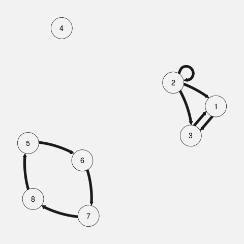
  Figure 1: Scenario 2. True interaction graph between the $K=8$ neurons. A directed edge is plotted from vertex $\ell$ to vertex $k$ if the interaction functions $h_{k,\ell}$ is non-null.

• Scenario 3: Setting $K=2$, we consider non piecewise constant interactions functions defined as:

  $$\begin{array}[]{cclccl}h_{1,1}(t)&=&100\cdot e^{-100t}\mathds{1}_{(0,0.04]}(t),&h_{2,1}(t)&=&30\cdot\mathds{1}_{(0,0.02]}(t)\\ h_{1,2}(t)&=&\frac{1}{2\times 0.004\sqrt{2\pi}}e^{-\frac{(t-0.02)^{2}}{2\times 0.004^{2}}}\cdot\mathds{1}_{(0,0.04]}(t),&h_{2,2}(t)&=&0.\end{array}$$

In all the scenarios, we consider $\nu_{\ell}=20,\ \ell=1,\dots,K$. For each scenario, we simulate $25$ datasets on the time interval $[0,22]$ seconds. The Bayesian inference is performed considering recordings on three possible periods of length $T=5$ seconds, $T=10$ seconds and $T=20$ seconds. For any dataset, we remove the initial period of $2$ seconds –corresponding to $50$ times the length of the support of the $h_{k,\ell}$-functions, assuming that, after this period, the Hawkes processes have reached their stationary distribution.

3.2 Prior distribution on $f=(\nu_{\ell},h_{k,\ell})_{l,k\in\{1,\dots,K\}}$

We use the prior distribution described in Section 2.3 setting a log-prior distribution on the $\nu_{\ell}$’s of parameter $\mu_{\nu},s^{2}_{\nu}$. About the interaction functions $\left(h_{k,\ell}\right)_{k,\ell\in\{1,\dots,K\}}$, the prior distribution is defined on the set of piecewise constant functions, $h_{k,\ell}$ being written as follows:

$$h_{k,\ell}(t)=\delta^{(k,\ell)}\sum_{j=1}^{J^{(k,\ell)}}\beta^{(k,\ell)}_{j}\mathds{1}_{[t^{(k,\ell)}_{j-1},t^{(k,\ell)}_{j}]}(t)$$ (3.1)

with $t^{(k,\ell)}_{0}=0$ and $t^{(k,\ell)}_{J^{(k,\ell)}}=A$. Using the notations in Section 2.3, we have $\beta^{(k,\ell)}_{j}=\rho^{(k,\ell)}\omega^{(k,\ell)}_{j}$. Here, $\delta^{(k,\ell)}$ is a global parameter of nullity for $h_{k,\ell}$ : for all $(k,\ell)\in\{1,\dots,K\}^{2}$,

$$\delta^{(k,\ell)}\sim_{i.i.d}\mathcal{B}ern(p).$$ (3.2)

For all $(k,\ell)\in\{1,\dots,K\}^{2}$, the number of steps $(J^{(k,\ell)})$ follows a translated Poisson prior distribution:

$$J^{(k,\ell)}|\{\delta^{(k,\ell)}=1\}\sim_{i.i.d.}1+\mathcal{P}(\eta).$$ (3.3)

To minimize the influence of $\eta$ on the posterior distribution, we consider an hyperprior distribution on the hyperparameter $\eta$:

$$\eta\sim\Gamma(a_{\eta},b_{\eta}).$$ (3.4)

Given $J^{(k,\ell)}$, we consider a spike and slab prior distribution on $(\beta^{(k,\ell)}_{j})_{j=1,\dots,J^{(k,\ell)}}$. Let $Z^{(k,\ell)}_{j}\in\{0,1\}$ denote a sign indicator for each step, we set: $\forall j\in\{1,\dots,J^{(k,\ell)}\}$:

$$\begin{array}[]{ccl}\mathbb{P}\left(Z^{(k,\ell)}_{j}=z|\delta^{(k,\ell)}=1\right)&=&\pi_{z},\quad\forall z\in\{0,1\}\\ \beta^{(k,\ell)}_{j}|\{\delta^{(k,\ell)}=1\}&\sim&Z^{(k,\ell)}_{j}\times\log\mathcal{N}(\mu_{\beta},s^{2}_{\beta}).\end{array}$$ (3.5)

We consider two prior distributions on $(t_{j}^{(k,\ell)})_{j=1\dots J^{(k,\ell)}}$. The first one (refered as the Regular histogram prior) is a regular partition of $[0,A]$:

$$t^{(k,\ell)}_{j}=\frac{j}{J^{(k,\ell)}}A\quad\quad\forall j=0,\dots,J^{(k,\ell)}.$$ (3.6)

The second prior distribution is refered as random histogram prior and specifies:

$$\begin{array}[]{ccl}(u_{1},\dots,u_{J^{(k,\ell)}})&\sim&\mathcal{D}(\alpha^{\prime}_{1},\dots\alpha^{\prime}_{J^{(k,\ell)}})\\ t^{(k,\ell)}_{0}&=&0\\ t^{(k,\ell)}_{j}&=&A\sum_{r=1}^{j}u_{r},\quad\forall j=1,\dots,J^{(k,\ell)}\end{array}$$ (3.7)

In the simulations studies, we set the following hyperparameters:

$$\begin{array}[]{cclcccl}\mu_{\beta}&=&3.5,&s_{\beta}&=&1\\ \mu_{\nu}&=&3.5,&s_{\nu}&=&1\\ \mathbb{P}(Z^{(k,\ell)}_{j}=1)&=&1/2,&\mathbb{P}(\delta^{(k,\ell)}=1)=p&=&1/2\\ \alpha^{\prime}_{j}&=&2,\quad\forall j\\ \end{array}$$

3.3 Posterior sampling

The posterior distribution is sampled using a standard Reversible-jump Markov chain Monte Carlo. Considering the current parameter $(\boldsymbol{\nu},\boldsymbol{h})$, $\boldsymbol{\nu}^{(c)}$ is proposed using a Metropolis-adjusted Langevin proposal. For a fixed $J^{(k,\ell)}$, the heights $\beta^{(k,\ell)}_{j}$ are proposed using a random walk proposing null or non-null candidates. Changes in the number of steps $J^{(k,\ell)}$ are proposed by standard birth and death moves (Green,, 1995). In this simulation study, we generate chains of length $30000$ removing the first $10000$ burn-in iterations. The algorithm is implemented in R on an Intel(R) Xeon(R) CPU E5-1650 v3 @ 3.50GHz.

The computation times (mean over the $25$ datasets) are given in Table 1. First note that the computation time increases roughly as a linear function of $T$. This is due to the fact that the heavier task in the algorithm is the integration of the conditional likelihood and the computation time of this operation is roughly a linear function of the length of the integration (observation) time interval. Besides, because we implemented a Reversible Jumps algorithm, the computation time is a stochastic quantity: the algorithm can explore parts of the domain where the number of bins $J_{\ell k}$ is large, thus increasing the computation time. This point can explain the unexpected computation times for $K=2$. Moreover, we remark that the computation time explodes as $K$ increases (due to the fact that $K^{2}$ intensity functions have to be estimated), reaching computation times greater than a day.

	K=2		K=8	K=2 with smooth $h_{k,\ell}$
Prior on $t$	Regular	Random	Regular	Random
T=5	1508.44	1002.45		823.84
T=10	1383.72	1459.55	37225.19	1284.93
T=20	2529.19	2602.48	49580.18	1897.17

Table 1: Mean computation time (in seconds) of the MCMC algorithms as a function of the scenario, the observation time interval and the prior distribution on $s$. The mean is computed over the $25$ simulated datasets

3.4 Results

We describe here the results for each scenario. We first present the $\mathbb{L}_{1}$-distances on $\lambda^{k}$ and $h_{k,\ell}$ for all $3$ the scenarios, all three length observation times $T$ and the two prior distributions. In Table 2, we show the estimated $\mathbb{L}_{1}$-distances on $\lambda^{k}$ and $h_{k,\ell}$. More precisely, we evaluate the $\mathbb{L}_{1}$-distances on the interactions functions

$$D^{(1)}=\frac{1}{25}\sum_{sim=1}^{25}\widehat{\mathbb{E}}\left[\frac{1}{K^{2}}\sum_{k,\ell=1}^{K}\left\|h_{k,\ell}-h^{0}_{k,\ell}\right\|_{1}\biggr{|}(N^{sim}_{t})_{t\in[0,T]}\right]$$

and the following stochastic distance :

$$D^{(2)}=\frac{1}{25}\sum_{sim=1}^{25}\widehat{\mathbb{E}}\left[d_{1,T}(f,f^{0}))\biggr{|}(N^{sim}_{t})_{t\in[0,T]}\right],$$

where $f^{0}$ is the true set of parameters, $d_{1,T}(f,f^{0})$ has been defined in Section  1.4 and the posterior expectations are approximated by Monte Carlo method using the outputs of the Reversible Jumps algorithm.

As expected, the error decreases as $T$ increases. As we will detail later, the random histogram prior gives better results than the regular prior. Finally, we perform better when the true interaction function $(h_{k,\ell})$ are step functions (due to the form of the prior distribution).

		K=2		K=8	K=2 with smooth $h_{k,\ell}$
	Prior	Regular	random	Regular	random
$D^{(}1)$: stochastic distances	T=5	11.59	9.59		11.75
	T=10	7.49	6.32	5.65	9.48
	T=20	5.40	4.11	3.17	7.9
$D^{(}2)$: distances on $h_{k,\ell}$	T=5	0.1423	0.0996		0.1431
	T=10	0.0844	0.0578	0.1199	0.1131
	T=20	0.0564	0.0336	0.0616	0.0945

Table 2: $\mathbb{L}_{1}$-distances on $h_{k,\ell}$ and $\lambda^{k}$

3.4.1 Results for scenario 1: $K=2$ with step functions

When $K=2$, we estimate the parameters using both regular and random prior distributions on $(t^{(k,\ell)}_{j})$ (equations (3.6) and (3.7)). One typical posterior distribution of $\nu_{\ell}$ is given in Figure 3 (left), for a randomly chosen dataset, clearly showing a smaller variance when the length of the observation interval increases. We also present the global estimation results, over the 25 simulated datasets. The distribution of the posterior mean estimators for $(\nu_{1},\nu_{2})$ computed for the 25 simulated datasets $\left(\widehat{\mathbb{E}}\left[\nu_{\ell}|(N^{sim}_{t})_{t\in[0,T]}\right]\right)_{sim=1\dots 25}$ is given in Figure 3 on the right panel, showing an expected decreasing variance for the estimator as $T$ increases. On the top panels the posterior is based on the regular grid prior while on the bottom the posterior is based on the random (grid) histogram prior: the results are equivalent.

About the estimation of the interaction functions, for the same given dataset, the estimation of the $h_{k,\ell}$ is plotted in Figure 2 (upper panel) for the regular prior, with its credible interval. Its corresponding estimation with the random prior is given in Figure 2 (bottom panel). For both prior distributions, the functions are globally well estimated, showing a clear concentration when $T$ increases. The regions where the interaction functions are null are also well identified. The estimation given with the random histogram prior is in general better than the one supplied by the regular prior. This may be due to several factors. First, the random histogram prior leads to a sparser estimation than the regular one. Secondly, it is easier to design a proposal move in the Reversible Jump algorithm in the former case than in the latter context.

Moreover, the interaction graph is perfectly inferred since the posterior probability for $\delta^{(2,2)}$ to be $0$ is almost $1$. For the 25 dataset, we estimate the posterior probabilities $\widehat{\mathbb{P}}(\delta^{(k,\ell)}=1|(N^{sim}_{t})_{t\in[0,T]})$ for $k,\ell=1,2$ and $sim=1\dots 25$. In Table 3, we display the mean of these posterior quantities. Even for the shorter observation time interval ($T=5)$ these quantities –defining completely the connexion graph– are well recovered. These results are improved when $T$ increases. Once again, the random histogram prior (3.7) gives better results.

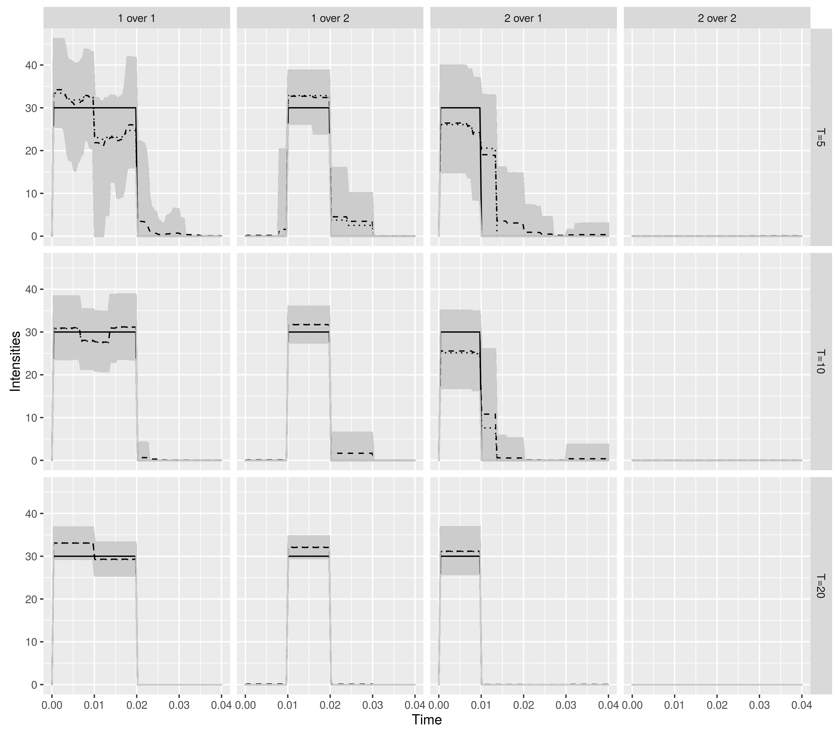
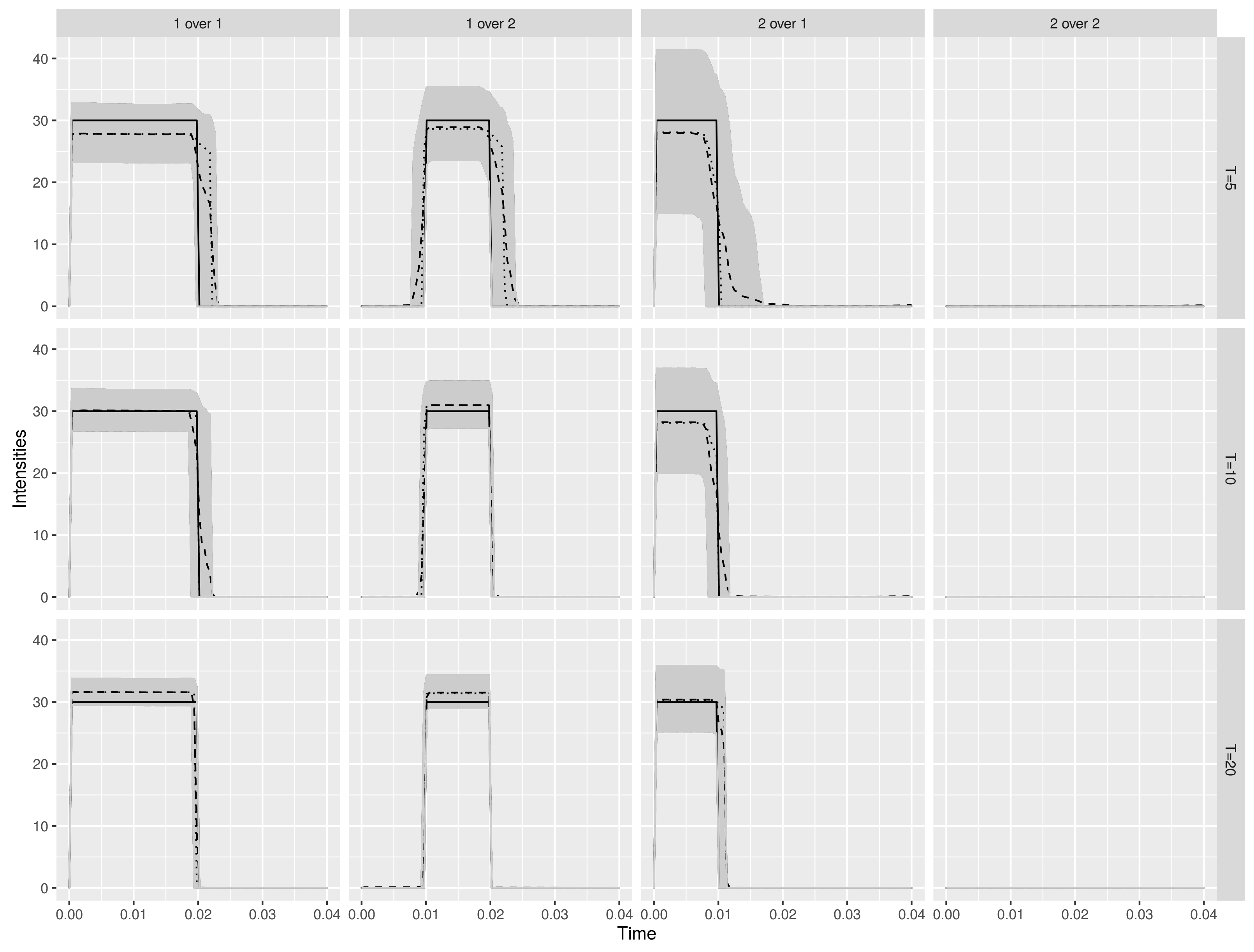
Figure 2: Results for scenario 1: Estimation of the $(h_{k,\ell})_{k,\ell=1,2}$ using the regular prior (upper panel) and the random histogram prior (bottom panel). The gray region indicates the credible region for $h_{k,\ell}(t)$ (delimited by the $5\%$ and $95\%$ percentiles of the posterior distribution). The true $h_{k,\ell}$ is in plain line, the posterior expectation and posterior median for $h_{k,\ell}(t)$ are in dotted and dashed lines respectively.

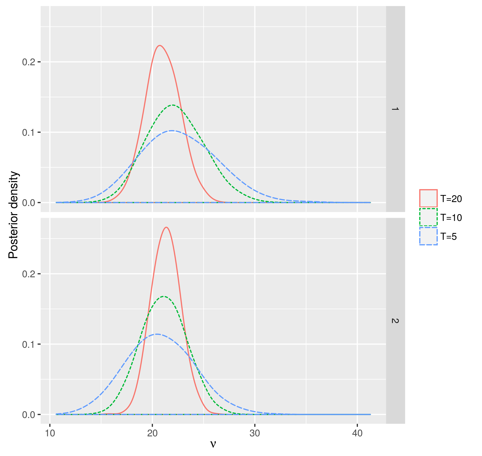
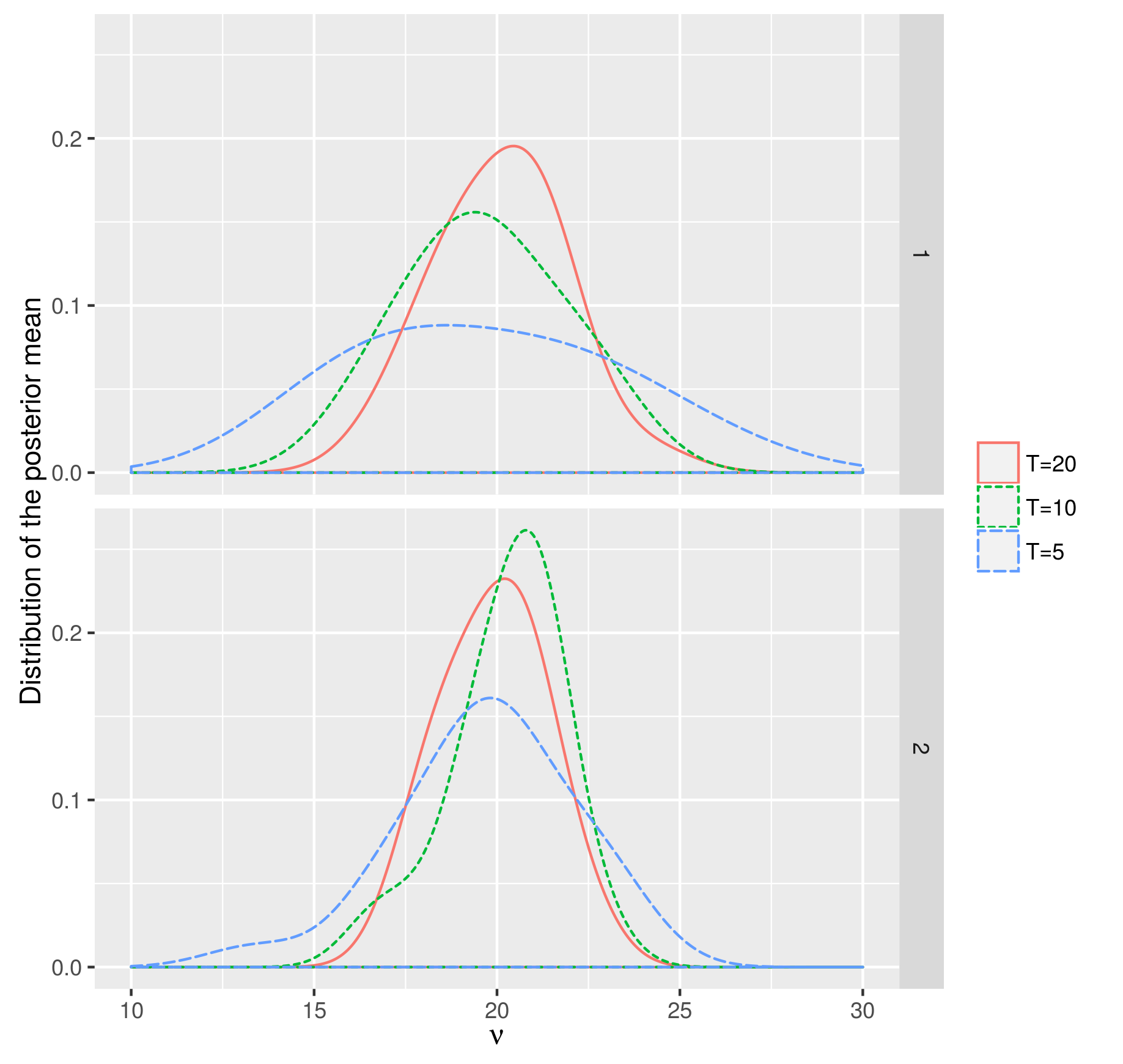
Figure 3: Results for scenario 1: On the left, posterior distribution of $(\nu_{1},\nu_{2})$ with $T=5$, $T=10$ and $T=20$ for one dataset. On the right, distribution of the posterior mean of $(\nu_{1},\nu_{2})$ $\left(\widehat{\mathbb{E}}\left[\nu_{\ell}|(N^{sim}_{t})_{t\in[0,T]}\right]\right)_{sim=1\dots 25}$ over the 25 simulated datasets. Top : regular histogram; bottom : random histogram

$\ell$ over $k$		$1$ over $1$	$1$ over $2$	$2$ over $1$	$2$ over $2$
True value of $\delta^{(k,\ell)}$		$1$	$1$	$1$	$0$
	Prior
$T=5$	Regular	1.0000	0.8970	1.0000	0.0071
	Continous	1.0000	0.9812	1.0000	0.0196
$T=10$	Regular	1.0000	0.9954	1.0000	0.0047
	Continous	1.0000	1.0000	1.0000	0.0102
$T=20$	Regular	1.0000	1.0000	1.0000	0.0099
	random	1.0000	1.0000	1.0000	0.0102

Table 3: Scenario 1, K=2. Mean of the posterior estimations: $\frac{1}{25}\sum_{sim=1}^{25}\widehat{\mathbb{P}}(\delta^{(k,\ell)}=1|(N^{sim}_{t})_{t\in[0,T]})$, for the three observation time intervals and the two prior distributions.

Finally, we also have a look at the conditional intensities $\lambda^{k}_{t}=\nu_{k}+\sum_{\ell=1}^{K}\int_{-\infty}^{t-}h_{\ell,k}(t-u)dN^{(\ell)}_{u}$. On Figure 4, we plot $50$ realizations of the conditional intensity from the posterior distributions. More precisely, for one given dataset, for $50$ parameters $\theta^{(i)}=\left((h^{(i)}_{k,\ell})_{k,\ell},(\nu^{(i)}_{k})_{k=1\dots K}\right)$ sampled from the posterior distribution (obtained at the end of the MCMC chain), we compute the corresponding $(\lambda^{k(i)}_{t})$ and plot them. For the sake of clarity, only the conditional intensity of the first process ($k=1$) is plotted and we restrict the graph to a short time interval $[3.2,3.6]$. As noticed before, the conditional intensity is well reconstructed, with a clear improvement of the precision as the length of the observation time $T$ increases.

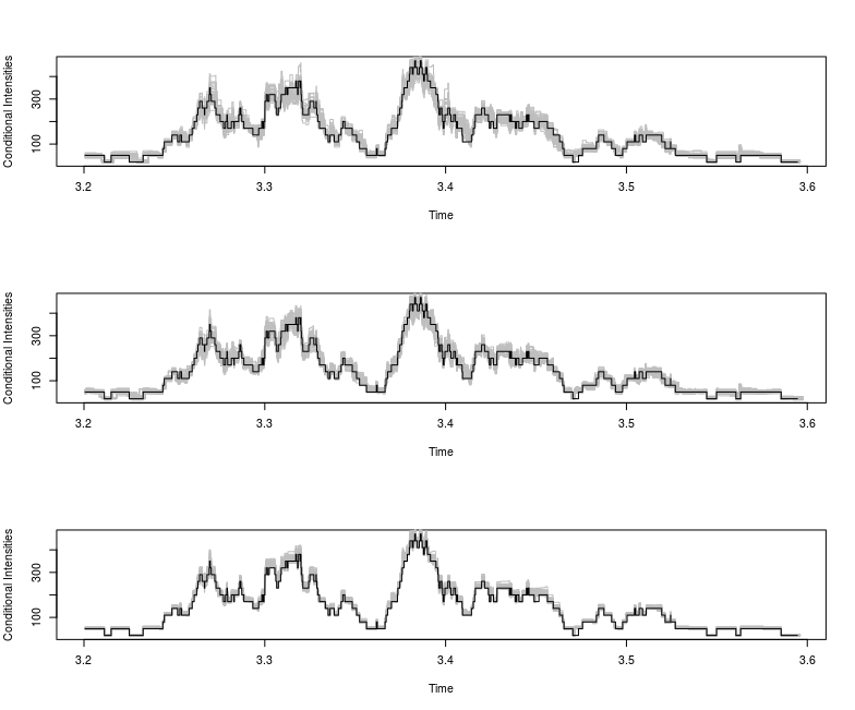
Figure 4: Scenario 1. Conditional intensity $\lambda^{1}_{t}$ : 50 realizations of $\lambda^{1}_{t}$ from the posterior distribution for one particular dataset and $3$ lengths of observation interval ($T=5$ on the first row $T=10$ on the second row, and $T=20$ on the third row). True conditional intensity in black plain line.

3.4.2 Results for scenario 2: $K=8$

In this scenario, we perform the Bayesian inference using only the regular prior distribution on $(\textbf{t}^{(k,\ell)})_{(k,\ell)\in\{1,\dots,K\}^{2}}$ and two lengths of observation interval ($T=10$ and $T=20$). Here we set $a_{\eta}=3$ and $b_{\eta}=1$.

The posterior distribution of the $(\nu_{k})_{k=1\dots K}$ for a randomly chosen dataset is plotted in Figure 5. The prior distribution is in dotted line and is flat. The posterior distribution concentrates around the true value (here $20$) with a smaller variance when $T$ increases.

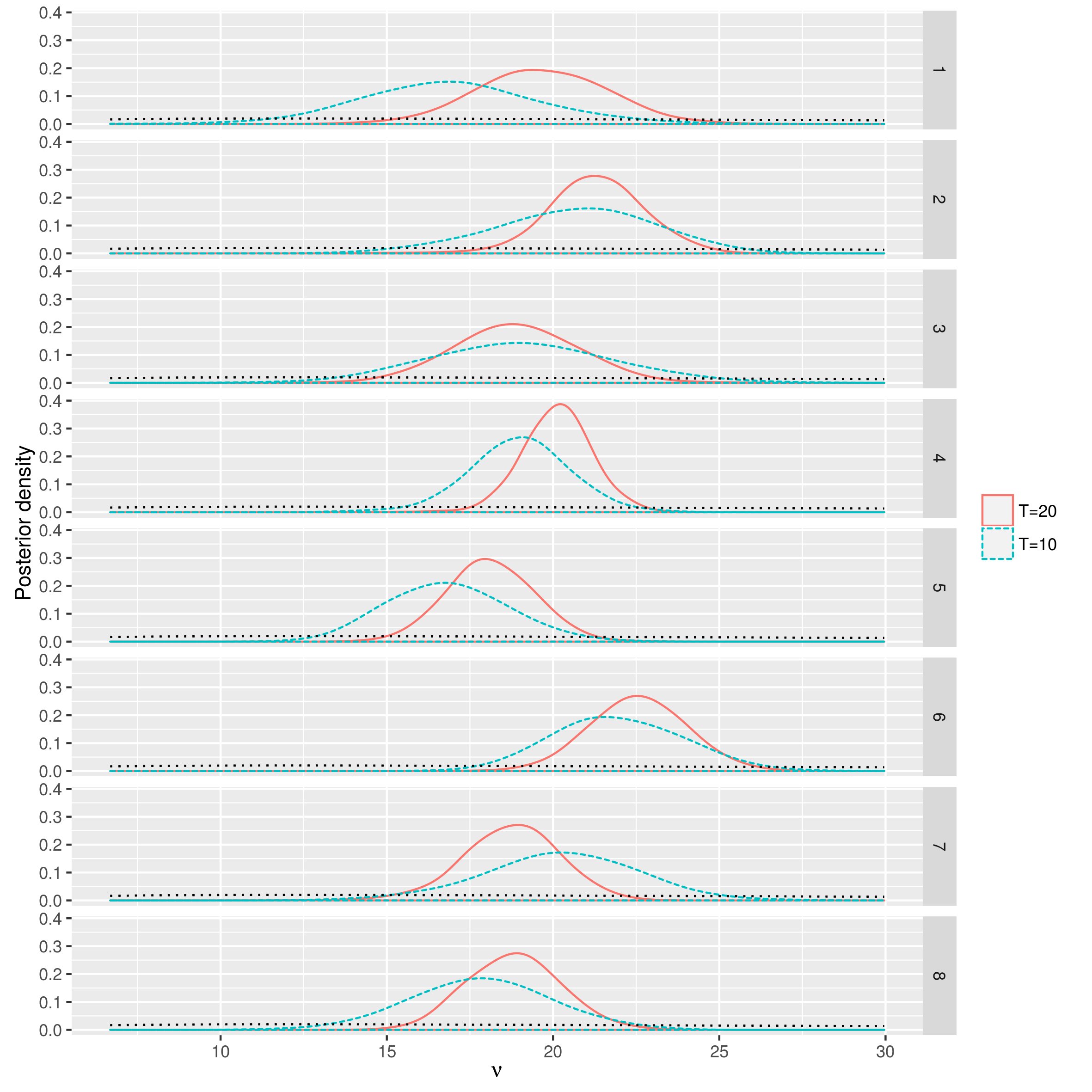
Figure 5: Scenario 2: Results on $(\nu_{\ell})_{k=1\dots K}$ for a particular dataset: Prior distribution (dotted line), Posterior distributions for $T=10$ ( dashed line) and $T=20$ (plain line)

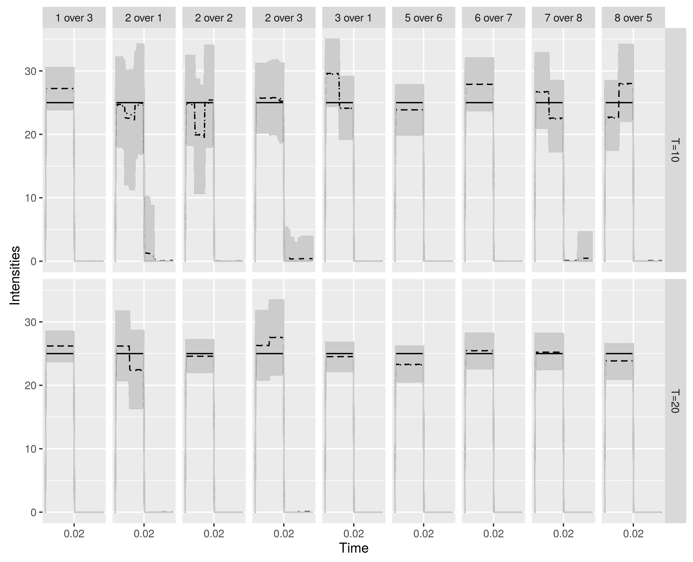
Figure 6: Scenario 2: Estimation of the non null interaction functions $(h_{k,\ell})_{k,\ell=1,\dots,8}$ using the regular prior for $T=10$ (upper panel) and $T=20$ (bottom). The gray region indicates the credible region for $h_{k,\ell}(t)$ (delimited by the $5\%$ and $95\%$ percentiles of the posterior distribution). The true $h_{k,\ell}$ is in plain line, the posterior expectation and posterior median for $h_{k,\ell}(t)$ are in dotted and dashed lines respectively (often undistinguishable).

In the context of neurosciences, we are especially interested in recovering the interaction graph of the $K=8$ neurons. In Figure 7, we consider the same dataset as the one used in Figure 5 and plot the posterior estimation of the interaction graph, for respectively $T=10$ on the left and $T=20$ on the right. The width and the gray level of the edges are proportional to the estimated posterior probability $\widehat{\mathbb{P}}(\delta^{(k,\ell)}=1|(N_{t})_{t\in[0,T]})$. The global structure of the graph is recovered (to be compared to the true graph plotted in Figure 1). We observe that the false positive edges appearing when $T=10$ disappear when $T=20$. In Figure 8, we consider the mean of the estimates of the graph over the 25 datasets. The resulting graph for $T=10$ is on the left and for $T=20$ on the right.

Note that, in this example, for any $(k,\ell)$ such that the true $\delta^{(k,\ell)}=1$, the estimated posterior probability $\widehat{\mathbb{P}}(\delta^{(k,\ell)}=1|(N^{sim}_{t})_{t\in[0,T]})$ is equal to $1$, for any dataset and any length of observation interval. In other words, the non-null interactions are perfectly recovered. In a simulation scenario with other interaction functions, the results could have been different.

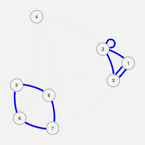
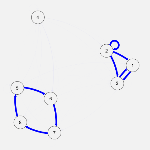
Figure 7: Results for scenario 2 for one given dataset: Posterior estimation of the interaction graph for $T=10$ on the left and $T=20$ on the right, for one randomly chosen dataset. Level of grey and width of the edges proportional to the posterior estimated probability of $\widehat{\mathbb{P}}(\delta^{(k,\ell)}=1|(N^{sim}_{t})_{t\in[0,T]})$.

Figure 8: Results for scenario 2 over the $25$ simulated datasets: Posterior estimation of the interaction graph for $T=10$ on the left and $T=20$ on the right. Level of grey and width of the edges are proportional to the posterior estimated probability of $\frac{1}{25}\sum_{sim=1}^{25}\widehat{\mathbb{P}}(\delta^{(k,\ell)}=1|(N^{sim}_{t})_{t\in[0,T]})$.

In Figure 6, we plot the posterior means (with credible regions) of the non-null interaction functions for the same simulated dataset as in Figure 7. The time intervals where the interaction functions are null are again perfectly recovered. The posterior incertainty around the non-null functions $h_{k,\ell}$ decreases when $T$ increases.

3.4.3 Results for scenario 3 : $K=2$ with smooth functions

In this context, we perform the inference using the random histogram prior distribution (3.7). In this case, we set $a_{\eta}=10$ and $b_{\eta}=1$. thus encouraging a greater number of step in the interactions functions. The behavior of the posterior distribution of $\nu_{k}$ is the same as in the other examples. In Figure 9, we plot the distribution of $\left(\mathbb{E}\left[\nu_{k}|(N^{sim}_{t})_{t\in[0,T]}\right]\right)_{sim=1\dots 25}$ for $T=5,10,20$ seconds and clearly observe a decrease of the biais and the variance as the length of the observation period increases. Some estimation of the interaction functions are given in Figure 10. Due to the choice of the prior distribution of these quantities, we get a sparse posterior inference.

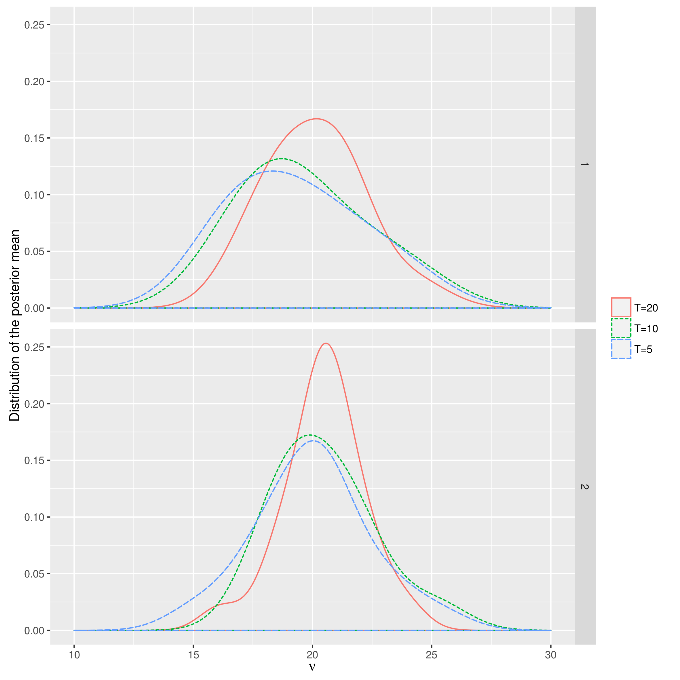
Figure 9: Results for scenario 3 : smooth interaction functions: Distributions of $\left(\mathbb{E}\left[\nu_{k}|(N^{sim}_{t})_{t\in[0,T]}\right]\right)_{sim=1\dots 25}$ for $T=5,10,20$ seconds (long dashed, short dashed and plain line respectively).

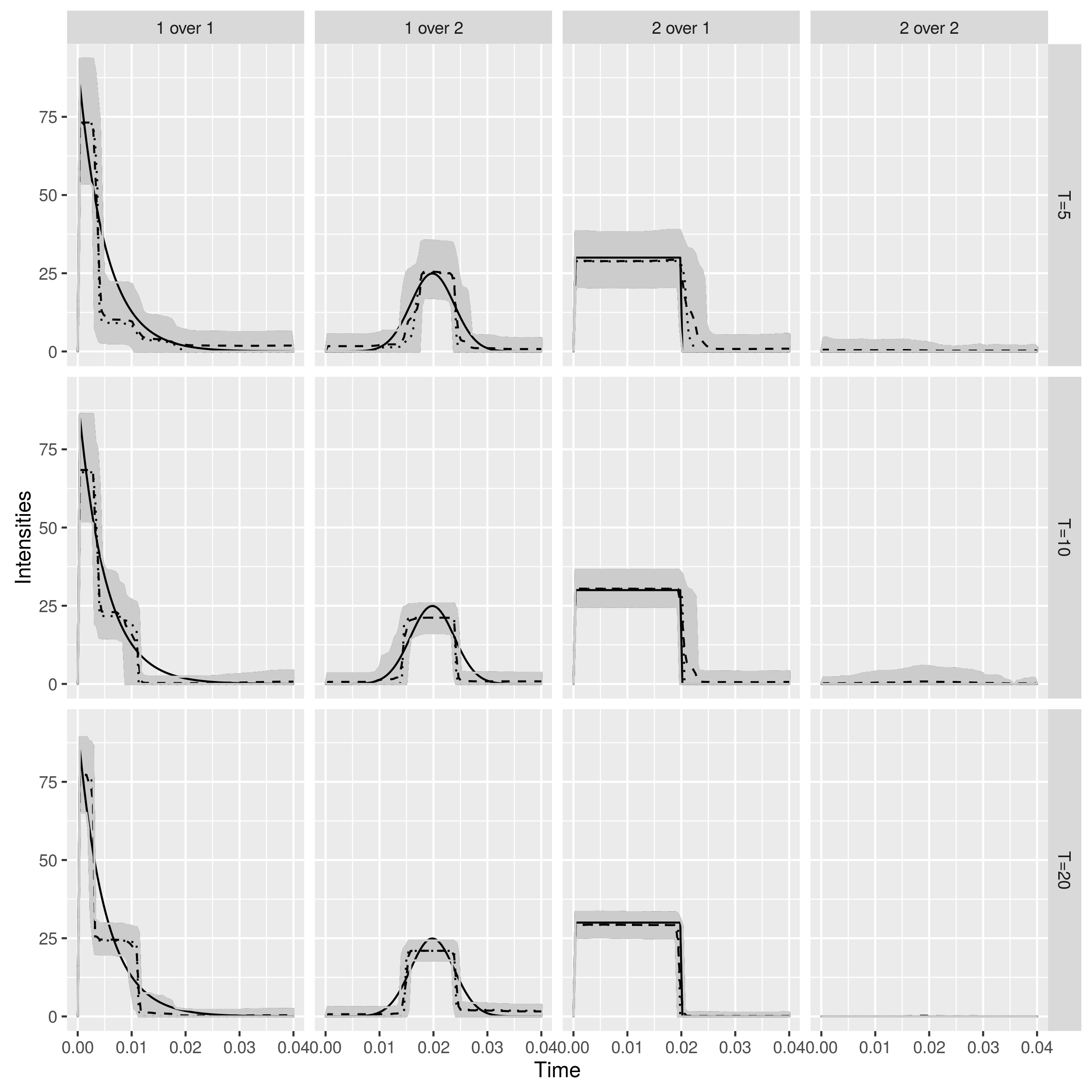
Figure 10: Results for scenario 3 : smooth interaction functions: Estimation of the interaction functions $(h_{k,\ell})_{k,\ell=1,2}$ using the regular prior for $T=10$ (upper panel) and $T=10$ (bottom). The gray region indicates the credible region for $h_{k,\ell}(t)$ (delimited by the $5\%$ and $95\%$ percentiles of the posterior distribution). The true $h_{k,\ell}$ is in plain line, the posterior expectation and posterior median for $h_{k,\ell}(t)$ are in dotted and dashed lines respectively (often undistinguishable).

4 Proofs of Theorems

4.1 Proof of Theorem 1

To prove Theorem 1, we apply the general methodology of Ghosal and van der Vaart, 2007a , with modifications due to the fact that $\exp(L_{T}(f))$ is the likelihood of the distribution of $(N^{k})_{k=1,\ldots,K}$ on $[0,T]$ conditional on $\mathcal{G}_{0^{-}}$ and that the metric $d_{1,T}$ depends on the observations. We set $M_{T}=M\sqrt{\log\log T}$, for $M$ a positive constant. Let

$$A_{\epsilon}=\{f\in{\mathcal{F}};\ d_{1,T}(f_{0},f)\leq K\epsilon\}$$

and for $j\geq 1$, we set

$$S_{j}=\left\{f\in\mathcal{F}_{T};\ d_{1,T}(f,f_{0})\in(Kj\epsilon_{T},K(j+1)\epsilon_{T}]\right\},$$ (4.1)

where $\mathcal{F}_{T}=\left\{f=((\nu_{k})_{k},(h_{k,\ell})_{k,\ell})\in\mathcal{F};\ (h_{k,\ell})_{k,\ell})\in\mathcal{H}_{T}\right\}$. So that, for any test function $\phi$,

$$\begin{split}\Pi\left(A_{M_{T}\epsilon_{T}}^{c}|N\right)&=\frac{\int_{A_{M_{T}\epsilon_{T}}^{c}}e^{L_{T}(f)-L_{T}(f_{0})}d\Pi(f)}{\int_{\mathcal{F}}e^{L_{T}(f)-L_{T}(f_{0})}d\Pi(f)}=:\frac{\bar{N}_{T}}{D_{T}}\\ &\leq\mathds{1}_{\Omega_{T}^{c}}+\mathds{1}_{\left\{D_{T}<\frac{\Pi(B(\epsilon_{T},T))}{\exp(2(\kappa_{T}+1)T\epsilon_{T}^{2})}\right\}}+\phi\mathds{1}_{\Omega_{T}}+\frac{e^{2(\kappa_{T}+1)T\epsilon_{T}^{2}}}{\Pi(B(\epsilon_{T},T))}\int_{{\mathcal{F}}_{T}^{c}}e^{L_{T}(f)-L_{T}(f_{0})}d\Pi(f)\\ &+\mathds{1}_{\Omega_{T}}\frac{e^{2(\kappa_{T}+1)T\epsilon_{T}^{2}}}{\Pi(B(\epsilon_{T},T))}\sum_{j=M_{T}}^{\infty}\int_{\mathcal{F}_{T}}\mathds{1}_{f\in S_{j}}e^{L_{T}(f)-L_{T}(f_{0})}(1-\phi)d\Pi(f)\end{split}$$

and

$$\begin{split}\mathbb{E}_{0}\left[\Pi\left(A_{M_{T}\epsilon_{T}}^{c}|N\right)\right]&\leq\mathbb{P}_{0}(\Omega_{T}^{c})+\mathbb{P}_{0}\left(D_{T}<e^{-2(\kappa_{T}+1)T\epsilon_{T}^{2}}\Pi(B(\epsilon_{T},B))\right)+\mathbb{E}_{0}[\phi\mathds{1}_{\Omega_{T}}]\\ &\quad+\frac{e^{2(\kappa_{T}+1)T\epsilon_{T}^{2}}}{\Pi(B(\epsilon_{T},B))}\left(\Pi(\mathcal{F}_{T}^{c})+\sum_{j=M_{T}}^{\infty}\int_{\mathcal{F}_{T}}\mathbb{E}_{0}\left[\mathbb{E}_{f}\left[\mathds{1}_{\Omega_{T}}\mathds{1}_{f\in S_{j}}(1-\phi)|\mathcal{G}_{0^{-}}\right]\right]d\Pi(f)\right),\end{split}$$

since

$$\mathbb{E}_{0}\left[\int_{{\mathcal{F}}_{T}^{c}}e^{L_{T}(f)-L_{T}(f_{0})}d\Pi(f)\right]=\mathbb{E}_{0}\left[\mathbb{E}_{0}\left[\int_{{\mathcal{F}}_{T}^{c}}e^{L_{T}(f)-L_{T}(f_{0})}d\Pi(f)|\mathcal{G}_{0^{-}}\right]\right]=\mathbb{E}_{0}\left[\mathbb{E}_{f}\left[\int_{{\mathcal{F}}_{T}^{c}}d\Pi(f)|\mathcal{G}_{0^{-}}\right]\right]=\Pi({\mathcal{F}}_{T}^{c}).$$

Since $e^{(\kappa_{T}+1)T\epsilon_{T}^{2}}e^{L_{T}(f)-L_{T}(f_{0})}\geq\mathds{1}_{\left\{L_{T}(f)-L_{T}(f_{0})\geq-(\kappa_{T}+1)T\epsilon_{T}^{2}\right\}},$

$$\begin{split}\mathbb{P}_{0}\left(D_{T}\leq e^{-2(\kappa_{T}+1)T\epsilon_{T}^{2}}\Pi(B(\epsilon_{T},B))\right)&\leq\mathbb{P}_{0}\left(\int_{B(\epsilon_{T},B)}e^{L_{T}(f)-L_{T}(f_{0})}\frac{d\Pi(f)}{\Pi(B(\epsilon_{T},B))}\leq e^{-2(\kappa_{T}+1)T\epsilon_{T}^{2}}\right)\\ &\leq\mathbb{P}_{0}\left(\int_{B(\epsilon_{T},B)}\mathds{1}_{\left\{L_{T}(f)-L_{T}(f_{0})\geq-(\kappa_{T}+1)T\epsilon_{T}^{2}\right\}}\frac{d\Pi(f)}{\Pi(B(\epsilon_{T},B))}\leq e^{-(\kappa_{T}+1)T\epsilon_{T}^{2}}\right)\\ &\leq\frac{\mathbb{E}_{0}\left[\int_{B(\epsilon_{T},B)}\mathds{1}_{\left\{L_{T}(f)-L_{T}(f_{0})<-(\kappa_{T}+1)T\epsilon_{T}^{2}\right\}}\frac{d\Pi(f)}{\Pi(B(\epsilon_{T},B))}\right]}{\left(1-e^{-(\kappa_{T}+1)T\epsilon_{T}^{2}}\right)}\\ &\leq\frac{\int_{B(\epsilon_{T},B)}\mathbb{P}_{0}\left(L_{T}(f_{0})-L_{T}(f)>(\kappa_{T}+1)T\epsilon_{T}^{2}\right)d\Pi(f)}{\Pi(B(\epsilon_{T},B))\left(1-e^{-(\kappa_{T}+1)T\epsilon_{T}^{2}}\right)}\\ &\lesssim\frac{\log\log(T)\log^{3}(T)}{T\epsilon_{T}^{2}},\end{split}$$

by using Lemma 2 of Section 4.4. Remember we have set $\rho_{k,\ell}^{0}:=\|h_{k,\ell}^{0}\|_{1}$ and $\rho_{k,\ell}:=\|h_{k,\ell}\|_{1}$. Since $h_{k,\ell}$ and $h^{0}_{k,\ell}$ are non-negative functions, $\int_{-s}^{A}h_{k,\ell}^{0}(u)du\leq\rho_{k,\ell}^{0},\quad\int_{0}^{T-s}h_{k,\ell}^{0}(u)du\leq\rho_{k,\ell}^{0},$ and note that

$$Td_{1,T}(f,f_{0}) = \sum_{\ell=1}^{K}\int_{0}^{T}\left|\nu_{\ell}-\nu_{\ell}^{0}+\sum_{k=1}^{K}\int_{t-A}^{t^{-}}(h_{k,\ell}-h_{k,\ell}^{0})(t-s)dN_{s}^{k}\right|dt$$

$$\geq \sum_{\ell=1}^{K}\left|\int_{0}^{T}\left(\nu_{\ell}-\nu_{\ell}^{0}+\sum_{k=1}^{K}\int_{t-A}^{t^{-}}(h_{k,\ell}-h_{k,\ell}^{0})(t-s)dN_{s}^{k}\right)dt\right|$$

$$\geq \sum_{\ell=1}^{K}\left|T(\nu_{\ell}-\nu_{\ell}^{0})+\int_{0}^{T}\left(\sum_{k=1}^{K}\int_{t-A}^{t^{-}}(h_{k,\ell}-h_{k,\ell}^{0})(t-s)dN_{s}^{k}\right)dt\right|,$$

then for any $\ell=1,\ldots,K$,

$$d_{1,T}(f,f_{0}) \geq \left|\nu_{\ell}-\nu_{\ell}^{0}+\frac{1}{T}\sum_{k=1}^{K}\int_{0}^{T}\int_{t-A}^{t^{-}}(h_{k,\ell}-h_{k,\ell}^{0})(t-s)dN_{s}^{k}dt\right|$$

$$= \left|\nu_{\ell}-\nu_{\ell}^{0}+\sum_{k=1}^{K}(\rho_{k,\ell}-\rho_{k,\ell}^{0})\frac{N^{k}[0,T-A]}{T}\right.$$

$$\left.+\frac{1}{T}\int_{-A}^{0}\int_{-s}^{A}(h_{k,\ell}-h_{k,\ell}^{0})(u)dudN_{s}^{k}+\frac{1}{T}\int_{T-A}^{T^{-}}\int_{0}^{T-s}(h_{k,\ell}-h_{k,\ell}^{0})(u)dudN_{s}^{k}\right|$$

$$= \left|\nu_{\ell}+\sum_{k=1}^{K}\rho_{k,\ell}\frac{N^{k}[0,T-A]}{T}+\frac{1}{T}\int_{-A}^{0}\int_{-s}^{A}h_{k,\ell}(u)dudN_{s}^{k}+\frac{1}{T}\int_{T-A}^{T^{-}}\int_{0}^{T-s}h_{k,\ell}(u)dudN_{s}^{k}\right.$$

$$-\left.\left(\nu_{\ell}^{0}+\sum_{k=1}^{K}\rho_{k,\ell}^{0}\frac{N^{k}[0,T-A]}{T}+\frac{1}{T}\int_{-A}^{0}\int_{-s}^{A}h_{k,\ell}^{0}(u)dudN_{s}^{k}+\frac{1}{T}\int_{T-A}^{T^{-}}\int_{0}^{T-s}h_{k,\ell}^{0}(u)dudN_{s}^{k}\right)\right|.$$

This implies for $f\in S_{j}$ that

$$\begin{split}&\nu_{\ell}+\sum_{k=1}^{K}\rho_{k,\ell}\frac{N^{k}[0,T-A]}{T}\leq\nu_{\ell}^{0}+\sum_{k=1}^{K}\rho_{k,\ell}^{0}\frac{N^{k}[-A,T]}{T}+K(j+1)\epsilon_{T}\\ &\nu_{\ell}+\sum_{k=1}^{K}\rho_{k,\ell}\frac{N^{k}[-A,T]}{T}\geq\nu_{\ell}^{0}+\sum_{k=1}^{K}\rho_{k,\ell}^{0}\frac{N^{k}[0,T-A]}{T}-K(j+1)\epsilon_{T}.\end{split}$$ (4.2)

On $\Omega_{T}$,

$$\sum_{k=1}^{K}\rho_{k,\ell}^{0}\frac{N^{k}[-A,T]}{T}\leq\sum_{k=1}^{K}\rho_{k,\ell}^{0}(\mu_{k}^{0}+\delta_{T}),$$

so that, for $T$ large enough, for all $j\geq 1$ $S_{j}\subset\mathcal{F}_{j}$ with

$$\mathcal{F}_{j}:=\{f\in\mathcal{F}_{T};\ \nu_{\ell}\leq\mu_{\ell}^{0}+1+Kj\epsilon_{T},\forall\ell\leq K\},$$

since

$$\mu_{\ell}^{0}=\nu_{\ell}^{0}+\sum_{k=1}^{K}\rho_{k,\ell}^{0}\mu_{k}^{0}.$$ (4.3)

Let $(f_{i})_{i=1,\ldots,{\mathcal{N}}_{j}}$ be the centering points of a minimal $\mathbb{L}_{1}$-covering of $\mathcal{F}_{j}$ by balls of radius $\zeta j\epsilon_{T}$ with $\zeta=1/(6N_{0})$ (with $N_{0}$ defined in Section 2) and define $\phi_{(j)}=\max_{i=1,\ldots,{\mathcal{N}}_{j}}\phi_{f_{i},j}$ where $\phi_{f_{i},j}$ is the individual test defined in Lemma 1 associated to $f_{i}$ and $j$ (see Section 4.3). Note also that there exists a constant $C_{0}$ such that

$${\mathcal{N}}_{j}\leq\left(C_{0}(1+j\epsilon_{T})/j\epsilon_{T}\right)^{K}{\mathcal{N}}(\zeta j\epsilon_{T}/2,\mathcal{H}_{T},\|.\|_{1})$$

where ${\mathcal{N}}(\zeta j\epsilon_{T}/2,\mathcal{H}_{T},\|.\|_{1})$ is the covering number of $\mathcal{H}_{T}$ by $\mathbb{L}_{1}$-balls with radius $\zeta j\epsilon_{T}/2$. There exists $C_{K}$ such that if $j\epsilon_{T}\leq 1$ then ${\mathcal{N}}_{j}\leq C_{K}e^{-K\log(j\epsilon_{T})}{\mathcal{N}}(\zeta j\epsilon_{T}/2,\mathcal{H}_{T},\|.\|_{1})$ and if $j\epsilon_{T}>1$ then ${\mathcal{N}}_{j}\leq C_{K}N(\zeta j\epsilon_{T}/2,\mathcal{H}_{T},\|.\|_{1})$. Moreover $j\mapsto{\mathcal{N}}(\zeta j\epsilon_{T}/2,\mathcal{H}_{T},\|.\|_{1})$ is monotone non-increasing, choosing $j\geq 2\zeta_{0}/\zeta$, we obtain that

$${\mathcal{N}}_{j}\leq C_{K}(\zeta/\zeta_{0})^{K}e^{K\log T}e^{x_{0}T\epsilon_{T}^{2}},$$

from hypothesis (iii) in Theorem 1. Combining this with Lemma 1, we have for all $j\geq 2\zeta_{0}/\zeta$,

$$\begin{split}\mathbb{E}_{0}[\mathds{1}_{\Omega_{T}}\phi_{(j)}]&\lesssim{\mathcal{N}}_{j}e^{-Tx_{2}(j\epsilon_{T}\wedge j^{2}\epsilon_{T}^{2})}\lesssim e^{K\log T}e^{x_{0}T\epsilon_{T}^{2}}e^{-x_{2}T(j\epsilon_{T}\wedge j^{2}\epsilon_{T}^{2})}\\ \sup_{f\in\mathcal{F}_{j}}\mathbb{E}_{0}\left[\mathbb{E}_{f}[\mathds{1}_{\Omega_{T}}\mathds{1}_{f\in S_{j}}(1-\phi_{(j)})|\mathcal{G}_{0^{-}}]\right]&\lesssim e^{-x_{2}T(j\epsilon_{T}\wedge j^{2}\epsilon_{T}^{2})},\end{split}$$

for $x_{2}$ a constant. Set $\phi=\max_{j\geq M_{T}}\phi_{(j)}$ with $M_{T}>2\zeta_{0}/\zeta$, then

$$\mathbb{E}_{0}[\mathds{1}_{\Omega_{T}}\phi]\lesssim e^{K\log T}e^{x_{0}T\epsilon_{T}^{2}}\left[\sum_{j=M_{T}}^{\lfloor\epsilon_{T}^{-1}\rfloor}e^{-x_{2}T\epsilon_{T}^{2}j^{2}}+\sum_{j\geq\epsilon_{T}^{-1}}e^{-Tx_{2}\epsilon_{T}j}\right]\lesssim e^{-x_{2}T\epsilon_{T}^{2}M_{T}^{2}/2}$$

and

$$\sum_{j=M_{T}}^{\infty}\int_{\mathcal{F}_{T}}\mathbb{E}_{0}\left[\mathbb{E}_{f}\left[\mathds{1}_{\Omega_{T}}\mathds{1}_{f\in S_{j}}(1-\phi)|\mathcal{G}_{0^{-}}\right]\right]d\Pi(f)\lesssim e^{-x_{2}T\epsilon_{T}^{2}M_{T}^{2}/2}.$$

Therefore,

$$\frac{e^{2(\kappa_{T}+1)T\epsilon_{T}^{2}}}{\Pi(B(\epsilon_{T},B))}\sum_{j=M_{T}}^{\infty}\int_{\mathcal{F}_{T}}\mathbb{E}_{0}\left[\mathbb{E}_{f}\left[\mathds{1}_{\Omega_{T}}\mathds{1}_{f\in S_{j}}(1-\phi)|\mathcal{G}_{0^{-}}\right]\right]d\Pi(f)=o(1)$$

if $M$ is a constant large enough, which terminates the proof of Theorem 1.

4.2 Proof of Theorem 2

The proof of Theorem 2 follows the same lines as for Theorem 1, except that the decomposition of $\mathcal{F}_{T}$ is based on the sets $\mathcal{F}_{j}$ and $\mathcal{H}_{T,i}$, $i\geq 1$ and $j\geq M_{T}$ for some $M_{T}>0$. For each $i\geq 1$, $j\geq M_{T}$, consider $S_{i,j}^{\prime}$ a maximal set of $\zeta j\epsilon_{T}$-separated points in $\mathcal{F}_{j}\cap\mathcal{H}_{T,i}$ (with a slight abuse of notations) and $\phi_{i,j}=\max_{f_{1}\in S_{i,j}^{\prime}}\phi_{f_{1}}$ with $\phi_{f_{1}}$ defined in Lemma 1. Then,

$$|S_{i,j}^{\prime}|\leq C_{K}(\zeta/\zeta_{0})^{K}e^{K\log(T)}{\mathcal{N}}(\zeta j\epsilon_{T}/2,\mathcal{H}_{T,i},\|.\|_{1}).$$

Setting $\bar{N}_{T,ij}:=\int_{\mathcal{F}_{T}\cap\mathcal{H}_{T,i}}\mathds{1}_{f\in S_{j}}e^{L_{T}(f)-L_{T}(f_{0})}d\Pi(f)$, using similar computations as for the proof of Theorem 1, we have:

$$\begin{split}\mathbb{E}_{0}\left[\Pi\left(A_{M_{T}\epsilon_{T}}^{c}|N\right)\right]&\leq\mathbb{P}_{0}(\Omega_{T}^{c})+\mathbb{P}_{0}\left(D_{T}<e^{-2(\kappa_{T}+1)T\epsilon_{T}^{2}}\Pi(B(\epsilon_{T},B))\right)+\frac{e^{2(\kappa_{T}+1)T\epsilon_{T}^{2}}}{\Pi(B(\epsilon_{T},B))}\Pi(\mathcal{F}_{T}^{c})\\ &+\mathbb{E}_{0}\left[\mathds{1}_{\Omega_{T}}\sum_{i=1}^{+\infty}\sum_{j=M_{T}}^{+\infty}\phi_{ij}\frac{\bar{N}_{T,ij}}{D_{T}}\right]+\frac{e^{2(\kappa_{T}+1)T\epsilon_{T}^{2}}}{\Pi(B(\epsilon_{T},B))}\mathbb{E}_{0}\left[\mathds{1}_{\Omega_{T}}\sum_{i=1}^{+\infty}\sum_{j=M_{T}}^{+\infty}(1-\phi_{ij})\bar{N}_{T,ij}\right].\end{split}$$

Assumptions of the theorem allow us to deal with the first three terms. So, we just have to bound the last two ones. Using the same arguments and the same notations as for Theorem 1,

$$\mathbb{E}_{0}\left[\mathds{1}_{\Omega_{T}}\sum_{i=1}^{+\infty}\sum_{j=M_{T}}^{+\infty}(1-\phi_{ij})\bar{N}_{T,ij}\right] = \sum_{i=1}^{+\infty}\int_{\mathcal{F}_{T}\cap\mathcal{H}_{T,i}}\sum_{j=M_{T}}^{+\infty}\mathbb{E}_{0}\left[\mathds{1}_{\Omega_{T}}\mathds{1}_{f\in S_{j}}(1-\phi_{ij})e^{L_{T}(f)-L_{T}(f_{0})}\right]d\Pi(f)$$

$$= \sum_{i=1}^{+\infty}\int_{\mathcal{F}_{T}\cap\mathcal{H}_{T,i}}\sum_{j=M_{T}}^{+\infty}\mathbb{E}_{0}\left[\mathbb{E}_{f}[\mathds{1}_{\Omega_{T}}\mathds{1}_{f\in S_{j}}(1-\phi_{ij})|\mathcal{G}_{0^{-}}]\right]d\Pi(f)$$

$$\lesssim \sum_{i=1}^{+\infty}\int_{\mathcal{F}_{T}\cap\mathcal{H}_{T,i}}d\Pi(f)\sum_{j=M_{T}}^{+\infty}e^{-x_{2}T(j\epsilon_{T}\wedge j^{2}\epsilon_{T}^{2})}\lesssim e^{-x_{2}T\epsilon_{T}^{2}M_{T}^{2}/2}.$$

Now, for $\gamma$ a fixed positive constant smaller than $x_{2}$, setting $\pi_{T,i}=\Pi(\mathcal{H}_{T,i})$, we have

$$\begin{split}&\mathbb{E}_{0}\left[\mathds{1}_{\Omega_{T}}\sum_{i=1}^{+\infty}\sum_{j=M_{T}}^{+\infty}\phi_{ij}\frac{\bar{N}_{T,ij}}{D_{T}}\right]\leq\mathbb{P}_{0}\left(D_{T}<e^{-2(\kappa_{T}+1)T\epsilon_{T}^{2}}\Pi(B(\epsilon_{T},B))\right)+\mathbb{P}_{0}\left(\exists(i,j);\sqrt{\pi_{T,i}}\phi_{i,j}>e^{-\gamma T(j\epsilon_{T}\wedge j^{2}\epsilon_{T}^{2})}\cap\Omega_{T}\right)\\ &\qquad+\sum_{i=1}^{+\infty}\sum_{j=M_{T}}^{+\infty}e^{-\gamma T(j\epsilon_{T}\wedge j^{2}\epsilon_{T}^{2})}\sqrt{\pi_{T,i}}\frac{e^{2(\kappa_{T}+1)T\epsilon_{T}^{2}}}{\Pi(B(\epsilon_{T},B))}\mathbb{E}_{0}\left[\mathds{1}_{\Omega_{T}}\int_{\mathcal{F}_{T}}\mathds{1}_{f\in S_{j}}e^{L_{T}(f)-L_{T}(f_{0})}d\Pi(f|\mathcal{H}_{T,i})\right].\end{split}$$

Now,

$$\mathbb{P}_{0}\left(\exists(i,j);\sqrt{\pi_{T,i}}\phi_{i,j}>e^{-\gamma T(j\epsilon_{T}\wedge j^{2}\epsilon_{T}^{2})}\cap\Omega_{T}\right) \leq\sum_{i=1}^{+\infty}\sqrt{\pi_{T,i}}\sum_{j=M_{T}}^{+\infty}e^{\gamma T(j\epsilon_{T}\wedge j^{2}\epsilon_{T}^{2})}\mathbb{E}_{0}[\mathds{1}_{\Omega_{T}}\phi_{i,j}]$$

$$\lesssim\sum_{i=1}^{+\infty}\sqrt{\pi_{T,i}}\sum_{j=M_{T}}^{+\infty}e^{(\gamma-x_{2})T(j\epsilon_{T}\wedge j^{2}\epsilon_{T}^{2})+K\log(T)}{\mathcal{N}}(\zeta j\epsilon_{T}/2,\mathcal{H}_{T,i},\|.\|_{1})$$

$$\lesssim e^{(\gamma-x_{2})T\epsilon_{T}^{2}M_{T}^{2}/2}\sum_{i=1}^{+\infty}\sqrt{\pi_{T,i}}{\mathcal{N}}(\zeta_{0}\epsilon_{T},\mathcal{H}_{T,i},\|.\|_{1})=o(1).$$

But, we have

$$\mathbb{E}_{0}\left[\mathds{1}_{\Omega_{T}}\int_{\mathcal{F}_{T}}\mathds{1}_{f\in S_{j}}e^{L_{T}(f)-L_{T}(f_{0})}d\Pi(f|\mathcal{H}_{T,i})\right] \leq 1$$

and

$$\mathbb{E}_{0}\left[\mathds{1}_{\Omega_{T}}\sum_{i=1}^{+\infty}\sum_{j=M_{T}}^{+\infty}\phi_{ij}\frac{\bar{N}_{T,ij}}{D_{T}}\right] \lesssim \sum_{i=1}^{+\infty}\sqrt{\pi_{T,i}}e^{-\gamma T\epsilon_{T}^{2}M_{T}^{2}}\frac{e^{2(\kappa_{T}+1)T\epsilon_{T}^{2}}}{\Pi(B(\epsilon_{T},B))}+o(1)=o(1),$$

for $M$ a contant large enough. This terminates the proof of Theorem 2.

4.3 Construction of tests

As usual, the control of the posterior distributions is based on specific tests. We build them in the following lemma.

Lemma 1.

Let $j\geq 1$, $f_{1}\in\mathcal{F}_{j}$ and define the test

$$\phi_{f_{1},j}=\max_{\ell=1,\ldots,K}\left(\mathds{1}_{\{N^{\ell}(A_{1,\ell})-\Lambda^{\ell}(A_{1,\ell};f_{0})\geq jT\epsilon_{T}/8\}}\vee\mathds{1}_{\{N^{\ell}(A_{1,\ell}^{c})-\Lambda^{\ell}(A_{1,\ell}^{c};f_{0})\geq jT\epsilon_{T}/8\}}\right),$$

with for all $\ell\leq K$, $A_{1,\ell}=\{t\in[0,T];\,\lambda_{t}^{\ell}(f_{1})\geq\lambda_{t}^{\ell}(f_{0})\}$, $\Lambda^{\ell}(A_{1,\ell};f_{0})=\int_{0}^{T}\mathds{1}_{A_{1,\ell}}(t)\lambda_{t}^{\ell}(f_{0})dt$ and $\Lambda^{\ell}(A_{1,\ell}^{c};f_{0})=\int_{0}^{T}\mathds{1}_{A_{1,\ell}^{c}}(t)\lambda_{t}^{\ell}(f_{0})dt$. Then

$$\mathbb{E}_{0}\left[\mathds{1}_{\Omega_{T}}\phi_{f_{1},j}\right]+\sup_{\|f-f_{1}\|_{1}\leq j\epsilon_{T}/(6N_{0})}\mathbb{E}_{0}\left[\mathbb{E}_{f}\left[\mathds{1}_{\Omega_{T}}\mathds{1}_{f\in S_{j}}(1-\phi_{f_{1},j})|\mathcal{G}_{0^{-}}\right]\right]\leq(2K+1)\max_{\ell}e^{-x_{1,\ell}Tj\epsilon_{T}(\sqrt{\mu_{\ell}^{0}}\wedge j\epsilon_{T})},$$

with $N_{0}$ is defined in Section 2 and

$$x_{1,\ell}=\min\left(36,1/(4096\mu^{0}_{\ell}),1/\left(1024K\sqrt{\mu_{\ell}^{0}}\right)\right).$$

Proof of Lemma 1.

Let $j\geq 1$ and $f_{1}=((\nu_{k}^{1})_{k=1,\ldots,K},(h_{\ell,k}^{1})_{k,\ell=1,\ldots,K})\in\mathcal{F}_{j}$. Let $\ell\in\{1,\ldots,K\}$ and let

$$\phi_{j,A_{1,\ell}}=\mathds{1}_{\left\{N^{\ell}(A_{1,\ell})-\Lambda^{\ell}(A_{1,\ell};f_{0})\geq jT\epsilon_{T}/8\right\}}.$$

By using (4.3), observe that on the event $\Omega_{T}$,

$$\begin{split}\int_{0}^{T}\lambda^{\ell}_{s}(f_{0})ds&=\nu_{\ell}^{0}T+\sum_{k=1}^{K}\int_{0}^{T}\int_{s-A}^{s^{-}}h_{k,\ell}^{0}(s-u)dN_{u}^{k}ds\\ &\leq\nu_{\ell}^{0}T+\sum_{k=1}^{K}\int_{-A}^{T^{-}}\int_{0}^{T}\mathds{1}_{u<s\leq A+u}h_{k,\ell}^{0}(s-u)dsdN_{u}^{k}\end{split}$$

and for $T$ large enough,

$$\int_{0}^{T}\lambda_{s}^{\ell}(f_{0})ds\leq\nu_{\ell}^{0}T+\sum_{k=1}^{K}\rho_{k,\ell}^{0}N^{k}[-A,T]\leq 2T\mu_{\ell}^{0}.$$ (4.4)

Let $j\leq\sqrt{\mu_{\ell}^{0}}\epsilon_{T}^{-1}$ and $x=x_{1}j^{2}T\epsilon_{T}^{2}$, for $x_{1}$ a constant. We use inequality (7.7) of Hansen et al., (2015), with $\tau=T$, $H_{t}=1_{A_{1,\ell}}(t)$, $v=2T\mu_{\ell}^{0}$ and $M_{T}=N^{\ell}(A_{1,\ell})-\Lambda^{\ell}(A_{1,\ell};f_{0}).$ So,

$$\mathbb{P}_{0}\left(\left\{N^{\ell}(A_{1,\ell})-\Lambda^{\ell}(A_{1,\ell};f_{0})\geq\sqrt{2vx}+\frac{x}{3}\right\}\cap\Omega_{T}\right)\leq e^{-x_{1}j^{2}T\epsilon_{T}^{2}}.$$

If $x_{1}\leq 1/(1024\mu_{\ell}^{0})$ and $x_{1}\leq 36$, we have that

$$\sqrt{2vx}+\frac{x}{3}=2\sqrt{\mu_{\ell}^{0}x_{1}}jT\epsilon_{T}+\frac{x_{1}j^{2}T\epsilon_{T}^{2}}{3}\leq 2\sqrt{\mu_{\ell}^{0}x_{1}}\left(1+\frac{\sqrt{x_{1}}}{6}\right)jT\epsilon_{T}\leq\frac{jT\epsilon_{T}}{8}.$$ (4.5)

Then

$$\mathbb{P}_{0}\left(\left\{N^{\ell}(A_{1,\ell})-\Lambda^{\ell}(A_{1,\ell};f_{0})\geq\frac{jT\epsilon_{T}}{8}\right\}\cap\Omega_{T}\right)\leq e^{-x_{1}j^{2}T\epsilon_{T}^{2}}.$$

If $j\geq\sqrt{\mu_{\ell}^{0}}\epsilon_{T}^{-1}$, we apply the same inequality but with $x=x_{0}jT\epsilon_{T}$ with $x_{0}=\sqrt{\mu_{\ell}^{0}}\times x_{1}$. Then,

$$\sqrt{2vx}+\frac{x}{3}=2\sqrt{\mu_{\ell}^{0}x_{1}\sqrt{\mu_{\ell}^{0}}j\epsilon_{T}}T+\frac{x_{1}\sqrt{\mu_{\ell}^{0}}jT\epsilon_{T}}{3}\leq 2\sqrt{\mu_{\ell}^{0}x_{1}}jT\epsilon_{T}+\frac{x_{1}\sqrt{\mu_{\ell}^{0}}jT\epsilon_{T}}{3}\leq\frac{jT\epsilon_{T}}{8},$$

where we have used (4.5). It implies

$$\mathbb{P}_{0}\left(\left\{N^{\ell}(A_{1,\ell})-\Lambda^{\ell}(A_{1,\ell};f_{0})\geq\frac{jT\epsilon_{T}}{8}\right\}\cap\Omega_{T}\right)\leq e^{-x_{0}jT\epsilon_{T}}.$$

Finally $\mathbb{E}_{0}\left[\mathds{1}_{\Omega_{T}}\phi_{j,A_{1,\ell}}\right]\leq e^{-x_{1}Tj\epsilon_{T}(\sqrt{\mu_{\ell}^{0}}\wedge j\epsilon_{T})}.$ Now, assume that

$$\int_{A_{1,\ell}}(\lambda_{t}^{\ell}(f_{1})-\lambda_{t}^{\ell}(f_{0}))dt\geq\int_{A_{1,\ell}^{c}}(\lambda_{t}^{\ell}(f_{0})-\lambda_{t}^{\ell}(f_{1}))dt.$$

Then

$$\frac{\|\lambda^{\ell}(f_{1})-\lambda^{\ell}(f_{0})\|_{1}}{2}:=\frac{\int_{0}^{T}|\lambda^{\ell}_{t}(f_{1})-\lambda^{\ell}_{t}(f_{0})|dt}{2}\leq\int_{A_{1,\ell}}(\lambda_{t}^{\ell}(f_{1})-\lambda_{t}^{\ell}(f_{0}))dt.$$ (4.6)

Let $f=((\nu_{k})_{k=1,\ldots,K},(h_{\ell,k})_{k,\ell=1,\ldots,K})\in S_{j}$ satisyfing $\|f-f_{1}\|_{1}\leq\zeta j\epsilon_{T}$ for some $\zeta>0$. Then,

$$\begin{split}\|\lambda^{\ell}(f)-\lambda^{\ell}(f_{1})\|_{1}&\leq T|\nu_{\ell}-\nu_{\ell}^{1}|+\int_{0}^{T}\left|\int_{t-A}^{t^{-}}\sum_{k}(h_{k,\ell}-h_{k,\ell}^{1})(t-u)dN^{k}_{u}\right|dt\\ &\leq T|\nu_{\ell}-\nu_{\ell}^{1}|+\sum_{k}\int_{0}^{T}\int_{t-A}^{t^{-}}|(h_{k,\ell}-h_{k,\ell}^{1})(t-u)|dN^{k}_{u}dt\\ &\leq T|\nu_{\ell}-\nu_{\ell}^{1}|+\max_{k}N^{k}[-A,T]\sum_{k}\|h_{k,\ell}-h_{k,\ell}^{1}\|_{1}\leq TN_{0}\|f-f_{1}\|_{1}\end{split}$$ (4.7)

and $\|\lambda^{\ell}(f)-\lambda^{\ell}(f_{1})\|_{1}\leq TN_{0}\zeta j\epsilon_{T}$. Since $f\in S_{j}$, there exists $\ell$ (depending on $f$) such that

$$\|\lambda^{\ell}(f)-\lambda^{\ell}(f_{0})\|_{1}\geq jT\epsilon_{T}.$$

This implies in particular that if $N_{0}\zeta<1$,

$$\begin{split}\|\lambda^{\ell}(f_{1})-\lambda^{\ell}(f_{0})\|_{1}&\geq\|\lambda^{\ell}(f)-\lambda^{\ell}(f_{0})\|_{1}-TN_{0}\zeta j\epsilon_{T}\geq(1-N_{0}\zeta)Tj\epsilon_{T}.\end{split}$$

We then have

$$\begin{split}\Lambda^{\ell}(A_{1,\ell};f)-\Lambda^{\ell}(A_{1,\ell};f_{0})&=\Lambda^{\ell}(A_{1,\ell};f)-\Lambda^{\ell}(A_{1,\ell};f_{1})+\Lambda^{\ell}(A_{1,\ell};f_{1})-\Lambda^{\ell}(A_{1,\ell};f_{0})\\ &\geq-\|\lambda^{\ell}(f)-\lambda^{\ell}(f_{1})\|_{1}+\int_{A_{1,\ell}}(\lambda_{t}^{\ell}(f_{1})-\lambda_{t}^{\ell}(f_{0}))dt\\ &\geq-\|\lambda^{\ell}(f)-\lambda^{\ell}(f_{1})\|_{1}+\frac{\|\lambda^{\ell}(f_{1})-\lambda^{\ell}(f_{0})\|_{1}}{2}\\ &\geq-TN_{0}\zeta j\epsilon_{T}+\frac{(1-N_{0}\zeta)Tj\epsilon_{T}}{2}=(1/2-3N_{0}\zeta/2)Tj\epsilon_{T}.\end{split}$$

Taking $\zeta=1/(6N_{0})$ leads to

$$\mathbb{E}_{f}\left[\mathds{1}_{f\in S_{j}}(1-\phi_{j,A_{1,\ell}})\mathds{1}_{\Omega_{T}}|\mathcal{G}_{0^{-}}\right] = \mathbb{E}_{f}\left[\mathds{1}_{f\in S_{j}}\mathds{1}_{\left\{N^{\ell}(A_{1,\ell})-\Lambda^{\ell}(A_{1,\ell};f_{0})<jT\epsilon_{T}/8\right\}}\mathds{1}_{\Omega_{T}}|\mathcal{G}_{0^{-}}\right]$$

$$\leq \mathbb{E}_{f}\left[\mathds{1}_{f\in S_{j}}\mathds{1}_{\left\{N^{\ell}(A_{1,\ell})-\Lambda^{\ell}(A_{1,\ell};f)\leq-jT\epsilon_{T}/8\right\}}\mathds{1}_{\Omega_{T}}|\mathcal{G}_{0^{-}}\right]$$

$$\leq \mathbb{E}_{f}\left[\mathds{1}_{\left\{N^{\ell}(A_{1,\ell})-\Lambda^{\ell}(A_{1,\ell};f)\leq-jT\epsilon_{T}/8\right\}}\mathds{1}_{\Omega_{T}}|\mathcal{G}_{0^{-}}\right].$$

Note that we can adapt inequality (7.7) of Hansen et al., (2015), with $H_{t}=\mathds{1}_{A_{1,\ell}}(t)$ to the case of conditional probability given $\mathcal{G}_{0^{-}}$ since the process $E_{t}$ defined in the proof of Theorem 3 of Hansen et al., (2015), being a supermartingale, satisfies $\mathbb{E}_{f}[E_{t}|\mathcal{G}_{0^{-}}]\leq E_{0}=1$ and, given that from (4.2) and (4.4),

$$\int_{0}^{T}\lambda^{\ell}_{s}(f)ds\leq\nu_{\ell}T+\sum_{k=1}^{K}\rho_{k,\ell}N^{k}[-A,T]\leq 2T\mu_{\ell}^{0}+K(j+1)T\epsilon_{T}=:\tilde{v}$$

for $T$ large enough, we obtain:

$$\mathbb{E}_{f}\left[\mathds{1}_{\left\{N^{\ell}(A_{1,\ell})-\Lambda^{\ell}(A_{1,\ell};f)\leq-\sqrt{2\tilde{v}x}-\frac{x}{3}\right\}}\mathds{1}_{\Omega_{T}}|\mathcal{G}_{0^{-}}\right]\leq e^{-x}.$$

We use the same computations as before, observing that $\tilde{v}=v+K(j+1)T\epsilon_{T}$.
If $j\leq\sqrt{\mu_{\ell}^{0}}\epsilon_{T}^{-1}$ we set $x=x_{1}j^{2}T\epsilon_{T}^{2}$, for $x_{1}$ a constant. Then,

$$\sqrt{2\tilde{v}x}+\frac{x}{3} \leq \sqrt{2vx}+\frac{x}{3}+\sqrt{2K(j+1)T\epsilon_{T}x}$$

$$\leq 2\sqrt{\mu_{\ell}^{0}x_{1}}jT\epsilon_{T}+\frac{x_{1}j^{2}T\epsilon_{T}^{2}}{3}+\sqrt{2K(j+1)\epsilon_{T}x_{1}}jT\epsilon_{T}$$

$$\leq 2\sqrt{\mu_{\ell}^{0}x_{1}}\left(1+\frac{\sqrt{x_{1}}}{6}\right)jT\epsilon_{T}+2\sqrt{Kj\epsilon_{T}x_{1}}jT\epsilon_{T}$$

$$\leq \left(2\sqrt{\mu_{\ell}^{0}x_{1}}\left(1+\frac{\sqrt{x_{1}}}{6}\right)+2\sqrt{K\sqrt{\mu_{\ell}^{0}}x_{1}}\right)jT\epsilon_{T}.$$

Therefore, if $x_{1}\leq\min\left(36,1/(4096\mu^{0}_{\ell}),1/\left(1024K\sqrt{\mu_{\ell}^{0}}\right)\right)$, then

$$\sqrt{2\tilde{v}x}+\frac{x}{3}\leq\frac{jT\epsilon_{T}}{8}.$$

If $j\geq\sqrt{\mu_{\ell}^{0}}\epsilon_{T}^{-1}$, we set $x=x_{0}jT\epsilon_{T}$ with $x_{0}=\sqrt{\mu_{\ell}^{0}}\times x_{1}$. Then,

$$\sqrt{2\tilde{v}x}+\frac{x}{3} \leq \sqrt{2vx}+\frac{x}{3}+\sqrt{2K(j+1)T\epsilon_{T}x}$$

$$\leq 2\sqrt{\mu_{\ell}^{0}x_{1}\sqrt{\mu_{\ell}^{0}}j\epsilon_{T}}T+\frac{x_{1}\sqrt{\mu_{\ell}^{0}}jT\epsilon_{T}}{3}+\sqrt{2K(j+1)T\epsilon_{T}\sqrt{\mu_{\ell}^{0}}x_{1}jT\epsilon_{T}}$$

$$\leq 2\sqrt{\mu_{\ell}^{0}x_{1}}jT\epsilon_{T}+\frac{x_{1}\sqrt{\mu_{\ell}^{0}}jT\epsilon_{T}}{3}+2\sqrt{K\sqrt{\mu_{\ell}^{0}}x_{1}}jT\epsilon_{T}\leq\frac{jT\epsilon_{T}}{8}.$$

Therefore,

$$\mathbb{E}_{f}\left[\mathds{1}_{\left\{N^{\ell}(A_{1,\ell})-\Lambda^{\ell}(A_{1,\ell};f)\leq-jT\epsilon_{T}/8\right\}}\mathds{1}_{\Omega_{T}}|\mathcal{G}_{0^{-}}\right]\leq e^{-x_{1}Tj\epsilon_{T}(\sqrt{\mu_{\ell}^{0}}\wedge j\epsilon_{T})}.$$

Now, if

$$\int_{A_{1,\ell}}(\lambda_{t}^{\ell}(f_{1})-\lambda_{t}^{\ell}(f_{0}))dt<\int_{A_{1,\ell}^{c}}(\lambda_{t}^{\ell}(f_{0})-\lambda_{t}^{\ell}(f_{1}))dt,$$

then

$$\int_{A_{1,\ell}^{c}}(\lambda_{t}^{\ell}(f_{1})-\lambda_{t}^{\ell}(f_{0}))dt\geq\frac{\|\lambda^{\ell}(f_{1})-\lambda^{\ell}(f_{0})\|_{1}}{2}$$

and the same computations are run with $A_{1,\ell}$ playing the role of $A_{1,\ell}^{c}$. This ends the proof of Lemma  1. ∎

4.4 Control of the denominator

The following lemma gives a control of $D_{T}$.

Lemma 2.

Let

$$KL(f_{0},f)=\mathbb{E}_{0}[L_{T}(f_{0})-L_{T}(f)].$$

On $B(\epsilon_{T},B)$,

$$0\leq KL(f_{0},f)\leq\kappa\log(r_{T}^{-1})T\epsilon_{T}^{2},$$ (4.8)

for $T$ larger than $T_{0}$, with $T_{0}$ some constant depending on $f_{0}$, with

$$\kappa=4\sum_{k=1}^{K}(\nu^{0}_{k})^{-1}\left(3+4K\sum_{\ell=1}^{K}\left(A\mathbb{E}_{0}[(\lambda^{\ell}_{0}(f_{0}))^{2}]+\mathbb{E}_{0}[\lambda^{\ell}_{0}(f_{0})]\right)\right)$$ (4.9)

and $r_{T}$ is defined in (4.11).

$$\mathbb{P}_{0}\left(L_{T}(f_{0})-L_{T}(f)\geq(\kappa\log(r_{T}^{-1})+1)T\epsilon_{T}^{2}\right)\leq\frac{C\log\log(T)\log^{3}(T)}{T\epsilon_{T}^{2}},$$ (4.10)

for $C$ a constant only depending on $f_{0}$ and $B$.

Proof.

We consider the set $\tilde{\Omega}_{T}$ defined in Lemma 3 and we set ${\mathcal{N}}_{T}=C_{\alpha}\log T$. We have:

$$KL(f^{0},f) = \sum_{k=1}^{K}\mathbb{E}_{0}\left[\int_{0}^{T}\log\left(\frac{\lambda_{t}^{k}(f_{0})}{\lambda_{t}^{k}(f)}\right)dN^{k}_{t}-\int_{0}^{T}\left(\lambda_{t}^{k}(f_{0})-\lambda_{t}^{k}(f)\right)dt\right]$$

$$= \sum_{k=1}^{K}\mathbb{E}_{0}\left[\int_{0}^{T}\log\left(\frac{\lambda_{t}^{k}(f_{0})}{\lambda_{t}^{k}(f)}\right)\lambda_{t}^{k}(f_{0})dt-\int_{0}^{T}\left(\lambda_{t}^{k}(f_{0})-\lambda_{t}^{k}(f)\right)dt\right]$$

$$= \sum_{k=1}^{K}\mathbb{E}_{0}\left[\int_{0}^{T}\Psi\left(\frac{\lambda_{t}^{k}(f)}{\lambda_{t}^{k}(f_{0})}\right)\lambda_{t}^{k}(f_{0})dt\right],$$

where for $u>0$, $\Psi(u):=-\log(u)-1+u\geq 0$. First, observe that on $\tilde{\Omega}_{T}\cap B(\epsilon_{T},B)$,

$$\frac{\lambda_{t}^{k}(f)}{\lambda_{t}^{k}(f_{0})}\geq\frac{\nu_{k}}{\nu^{0}_{k}+\sum_{\ell=1}^{K}\int_{t-A}^{t-}h^{0}_{\ell,k}(t-u)dN^{\ell}(u)}\geq\frac{\min_{k}\nu^{0}_{k}-\epsilon_{T}}{\max_{k}\nu^{0}_{k}+\max_{\ell,k}\|h_{\ell,k}^{0}\|_{\infty}K{\mathcal{N}}_{T}}=:r_{T}.$$ (4.11)

Furthermore, observe that for $u\in[r_{T},1/2)$, $\Psi(u)\leq\log(r_{T}^{-1})$, since $r_{T}=o(1)$. And for all $u\geq 1/2$, $\Psi(u)\leq(u-1)^{2}$. Finally, for any $u\geq r_{T}$,

$$\Psi(u)\leq 4\log(r_{T}^{-1})(u-1)^{2}.$$

Therefore, on $B(\epsilon_{T},B)$, we have

$$0\leq KL(f^{0},f) \leq 4\log(r_{T}^{-1})\sum_{k=1}^{K}\mathbb{E}_{0}\left[\int_{0}^{T}\frac{(\lambda_{t}^{k}(f_{0})-\lambda_{t}^{k}(f))^{2}}{\lambda_{t}^{k}(f_{0})}\mathds{1}_{\tilde{\Omega}_{T}}dt\right]+R_{T}$$

$$\leq 4\log(r_{T}^{-1})\sum_{k=1}^{K}(\nu^{0}_{k})^{-1}\mathbb{E}_{0}\left[\int_{0}^{T}(\lambda_{t}^{k}(f_{0})-\lambda_{t}^{k}(f))^{2}dt\right]+R_{T}$$

where

$$R_{T}=\sum_{k=1}^{K}\mathbb{E}_{0}\left[\mathds{1}_{\tilde{\Omega}_{T}^{c}}\int_{0}^{T}\left(-\log\left(\frac{\lambda_{t}^{k}(f)}{\lambda_{t}^{k}(f_{0})}\right)-1+\frac{\lambda_{t}^{k}(f)}{\lambda_{t}^{k}(f_{0})}\right)\lambda_{t}^{k}(f_{0})dt\right].$$

We first deal with the first term. Using stationarity of the process and Proposition 2 of Hansen et al., (2015)

$$\begin{split}\mathbb{E}_{0}\left[\int_{0}^{T}(\lambda_{t}^{k}(f_{0})-\lambda_{t}^{k}(f))^{2}dt\right]&\leq 2T(\nu^{0}_{k}-\nu_{k})^{2}+2\int_{0}^{T}\mathbb{E}_{0}\left[\left(\sum_{\ell=1}^{K}\int_{t-A}^{t^{-}}(h_{\ell,k}-h^{0}_{\ell,k})(t-u)dN^{\ell}(u)\right)^{2}\right]dt\\ &\leq 2T\epsilon_{T}^{2}+4K\int_{0}^{T}\mathbb{E}_{0}\left[\sum_{\ell=1}^{K}\left(\int_{t-A}^{t^{-}}(h_{\ell,k}-h^{0}_{\ell,k})(t-u)\lambda_{u}^{\ell}(f_{0})du\right)^{2}\right]dt\\ &\quad+4K\int_{0}^{T}\mathbb{E}_{0}\left[\sum_{\ell=1}^{K}\left(\int_{t-A}^{t^{-}}(h_{\ell,k}-h^{0}_{\ell,k})(t-u)\left(dN^{\ell}_{u}-\lambda_{u}^{\ell}(f_{0})du\right)\right)^{2}\right]dt\\ &\leq 2T\epsilon_{T}^{2}+4K\sum_{\ell=1}^{K}\|h_{\ell,k}-h^{0}_{\ell,k}\|_{2}^{2}\int_{0}^{T}\int_{t-A}^{t^{-}}\mathbb{E}_{0}[(\lambda_{u}^{\ell}(f_{0}))^{2}]dudt\\ &\quad+4K\int_{0}^{T}\sum_{\ell=1}^{K}\int_{t-A}^{t^{-}}(h_{\ell,k}-h^{0}_{\ell,k})^{2}(t-u)\mathbb{E}_{0}\left[\lambda_{u}^{\ell}(f_{0})\right]dudt\\ &\leq 2T\epsilon_{T}^{2}+4KT\sum_{\ell=1}^{K}\|h_{\ell,k}-h^{0}_{\ell,k}\|_{2}^{2}\left(A\mathbb{E}_{0}[(\lambda_{0}^{\ell}(f_{0}))^{2}]+\mathbb{E}_{0}[\lambda_{0}^{\ell}(f_{0})]\right)\\ &\leq T\epsilon_{T}^{2}\left(2+4K\sum_{\ell=1}^{K}\left(A\mathbb{E}_{0}[(\lambda_{0}^{\ell}(f_{0}))^{2}]+\mathbb{E}_{0}[\lambda_{0}^{\ell}(f_{0})]\right)\right).\end{split}$$

We now deal with $R_{T}$. We have, on $B(\epsilon_{T},B)$,

$$\frac{\lambda_{t}^{k}(f)}{\lambda_{t}^{k}(f_{0})} \leq (\nu_{k}^{0})^{-1}\left(\nu_{k}+\sum_{\ell=1}^{K}\|h_{\ell,k}\|_{\infty}\sup_{t\in[0,T]}N^{\ell}([t-A,t))\right)$$ (4.12)

$$\leq (\nu_{k}^{0})^{-1}\left(\nu^{0}_{k}+\epsilon_{T}+B\sum_{\ell=1}^{K}\sup_{t\in[0,T]}N^{\ell}([t-A,t))\right).$$ (4.13)

Conversely,

$$\frac{\lambda_{t}^{k}(f)}{\lambda_{t}^{k}(f_{0})}\geq(\nu_{k}^{0}-\epsilon_{T})\left(\nu^{0}_{k}+\sum_{\ell=1}^{K}\|h^{0}_{\ell,k}\|_{\infty}\sup_{t\in[0,T]}N^{\ell}([t-A,t))\right)^{-1}.$$ (4.14)

So, using Lemma 3, if $\alpha$ is an absolute constant large enough, $R_{T}=o(1)$ and

$$R_{T}=o(T\epsilon_{T}^{2}).$$

Choosing $\kappa=4\sum_{k=1}^{K}(\nu^{0}_{k})^{-1}\left(3+4K\sum_{\ell=1}^{K}\left(A\mathbb{E}_{0}[(\lambda^{\ell}_{0}(f_{0}))^{2}]+\mathbb{E}_{0}[\lambda^{\ell}_{0}(f_{0})]\right)\right)$ terminates the proof of (4.8). Note that if $B(\epsilon_{T},B)$ is replaced with $B_{\infty}(\epsilon_{T},B)$ (see Remark 1) then

$$\frac{\lambda_{t}^{k}(f)}{\lambda_{t}^{k}(f_{0})}\leq 1+\frac{|\nu_{k}-\nu_{k}^{0}|+\sum_{\ell}\|h_{\ell,k}-h_{\ell,k}\|_{\infty}\mathcal{N}_{T}}{\nu_{k}^{0}}$$

and

$$\frac{\lambda_{t}^{k}(f)}{\lambda_{t}^{k}(f_{0})}\geq 1-\frac{|\nu_{k}-\nu_{k}^{0}|+\sum_{\ell}\|h_{\ell,k}-h_{\ell,k}\|_{\infty}\mathcal{N}_{T}}{\nu_{k}^{0}}$$

so that we can take $r_{T}=1/2$ and $R_{T}=o(T\epsilon_{T}^{2})$.

We now study

$$\mathcal{L}_{T}:=L_{T}(f_{0})-L_{T}(f)-\mathbb{E}_{0}[L_{T}(f_{0})-L_{T}(f)].$$

We have for any integer $Q_{T}$ such that $x:=T/(2Q_{T})>A$,

$$L_{T}(f_{0})-L_{T}(f) = \sum_{k=1}^{K}\left(\int_{0}^{T}\log\left(\frac{\lambda_{t}^{k}(f_{0})}{\lambda_{t}^{k}(f)}\right)dN^{k}_{t}-\int_{0}^{T}\left(\lambda_{t}^{k}(f_{0})-\lambda_{t}^{k}(f)\right)dt\right)$$

$$= \sum_{q=0}^{Q_{T}-1}\int_{2qx}^{2qx+x}\sum_{k=1}^{K}\left(\log\left(\frac{\lambda_{t}^{k}(f_{0})}{\lambda_{t}^{k}(f)}\right)dN^{k}_{t}-\left(\lambda_{t}^{k}(f_{0})-\lambda_{t}^{k}(f)\right)dt\right)$$

$$\hskip 28.45274pt+\sum_{q=0}^{Q_{T}-1}\int_{2qx+x}^{2qx+2x}\sum_{k=1}^{K}\left(\log\left(\frac{\lambda_{t}^{k}(f_{0})}{\lambda_{t}^{k}(f)}\right)dN^{k}_{t}-\left(\lambda_{t}^{k}(f_{0})-\lambda_{t}^{k}(f)\right)dt\right)$$

$$=: \sum_{q=0}^{Q_{T}-1}F_{q}+\sum_{q=0}^{Q_{T}-1}\tilde{F}_{q}.$$

Note that $F_{q}$ is a measurable function of the points of $N$ appearing in $[2qx-A;2qx+x)$ denoted by $\mathcal{F}(N_{|[2qx-A;2qx+x)}).$ Using Proposition 3.1 of Reynaud-Bouret and Roy, (2006), we consider an i.i.d. sequence $(M_{q}^{x})_{q=0,\ldots,Q_{T}-1}$ of Hawkes processes with the same distribution as $N$ but restricted to $[2qx-A;2qx+x)$ and such that for all $q$, the variation distance between $M_{q}^{x}$ and $N_{|[2qx-A;2qx+x)}$ is less than $2\mathbb{P}_{0}(T_{e}>x-A)$, where $T_{e}$ is the extinction time of the process. We then set for any $q$,

$$G_{q}=\mathcal{F}(M_{q}^{x}).$$

We have built an i.i.d. sequence $(G_{q})_{q=0,\ldots,Q_{T}-1}$ with the same distributions as the $F_{q}$’s. Furthermore, for any $q$,

$$\mathbb{P}_{0}(F_{q}\not=G_{q})\leq 2\mathbb{P}_{0}(T_{e}>x-A).$$

We now have, by stationarity

$$\mathbb{P}_{0}(\mathcal{L}_{T}\geq T\epsilon_{T}^{2}) = \mathbb{P}_{0}\left(L_{T}(f_{0})-L_{T}(f)-\mathbb{E}_{0}[L_{T}(f_{0})-L_{T}(f)]\geq T\epsilon_{T}^{2}\right)$$

$$= \mathbb{P}_{0}\left(\sum_{q=0}^{Q_{T}-1}(F_{q}-\mathbb{E}_{0}[F_{q}])+\sum_{q=0}^{Q_{T}-1}(\tilde{F}_{q}-\mathbb{E}_{0}[\tilde{F}_{q}])\geq T\epsilon_{T}^{2}\right)$$

$$\leq 2\mathbb{P}_{0}\left(\sum_{q=0}^{Q_{T}-1}(F_{q}-\mathbb{E}_{0}[F_{q}])\geq T\epsilon_{T}^{2}/2\right)$$

$$\leq 2\mathbb{P}_{0}\left(\sum_{q=0}^{Q_{T}-1}(G_{q}-\mathbb{E}_{0}[G_{q}])\geq T\epsilon_{T}^{2}/2\right)+2\mathbb{P}_{0}\left(\exists q;\ F_{q}\not=G_{q}\right)$$

$$\leq 2\mathbb{P}_{0}\left(\sum_{q=0}^{Q_{T}-1}(G_{q}-\mathbb{E}_{0}[G_{q}])\geq T\epsilon_{T}^{2}/2\right)+4Q_{T}\mathbb{P}_{0}(T_{e}>x-A).$$

We first deal with the first term of the previous expression:

$$\mathbb{P}_{0}\left(\sum_{q=0}^{Q_{T}-1}(G_{q}-\mathbb{E}_{0}[G_{q}])\geq T\epsilon_{T}^{2}/2\right) \leq \frac{4}{T^{2}\epsilon_{T}^{4}}\mbox{Var}_{0}\left(\sum_{q=0}^{Q_{T}-1}G_{q}\right)$$

$$\leq \frac{4}{T^{2}\epsilon_{T}^{4}}\sum_{q=0}^{Q_{T}-1}\mbox{Var}_{0}\left(G_{q}\right)$$

$$\leq \frac{4Q_{T}}{T^{2}\epsilon_{T}^{4}}\mbox{Var}_{0}\left(G_{0}\right)=\frac{4Q_{T}}{T^{2}\epsilon_{T}^{4}}\mbox{Var}_{0}\left(F_{0}\right).$$

Now, by setting $d{\mathcal{M}}^{(k)}_{t}=dN^{k}_{t}-\lambda_{t}^{k}(f_{0})dt$,

$$\mbox{Var}_{0}\left(F_{0}\right) \leq \mathbb{E}_{0}\left[F_{0}^{2}\right]$$

$$\leq \mathbb{E}_{0}\left[\left(\sum_{k=1}^{K}\int_{0}^{\frac{T}{2Q_{T}}}\log\left(\frac{\lambda_{t}^{k}(f_{0})}{\lambda_{t}^{k}(f)}\right)dN^{k}_{t}-\sum_{k=1}^{K}\int_{0}^{\frac{T}{2Q_{T}}}(\lambda_{t}^{k}(f_{0})-\lambda_{t}^{k}(f))dt\right)^{2}\right]$$

$$\lesssim \sum_{k=1}^{K}\mathbb{E}_{0}\left[\left(\int_{0}^{\frac{T}{2Q_{T}}}\Psi\left(\frac{\lambda_{t}^{k}(f)}{\lambda_{t}^{k}(f_{0})}\right)\lambda_{t}^{k}(f_{0})dt+\int_{0}^{\frac{T}{2Q_{T}}}\log\left(\frac{\lambda_{t}^{k}(f_{0})}{\lambda_{t}^{k}(f)}\right)d{\mathcal{M}}^{(k)}_{t}\right)^{2}\right]$$

$$\lesssim \sum_{k=1}^{K}\mathbb{E}_{0}\left[\left(\int_{0}^{\frac{T}{2Q_{T}}}\Psi\left(\frac{\lambda_{t}^{k}(f)}{\lambda_{t}^{k}(f_{0})}\right)\lambda_{t}^{k}(f_{0})dt\right)^{2}\right]+\mathbb{E}_{0}\left[\left(\int_{0}^{\frac{T}{2Q_{T}}}\log\left(\frac{\lambda_{t}^{k}(f_{0})}{\lambda_{t}^{k}(f)}\right)d{\mathcal{M}}^{(k)}_{t}\right)^{2}\right]$$

$$\lesssim \sum_{k=1}^{K}\frac{T}{Q_{T}}\mathbb{E}_{0}\left[\int_{0}^{\frac{T}{2Q_{T}}}\Psi^{2}\left(\frac{\lambda_{t}^{k}(f)}{\lambda_{t}^{k}(f_{0})}\right)(\lambda_{t}^{k}(f_{0}))^{2}dt\right]+\mathbb{E}_{0}\left[\int_{0}^{\frac{T}{2Q_{T}}}\log^{2}\left(\frac{\lambda_{t}^{k}(f_{0})}{\lambda_{t}^{k}(f)}\right)\lambda^{k}_{t}(f_{0})dt\right].$$

Note that on $\tilde{\Omega}_{T}$, for any $t\in[0;T/(2Q_{T})]$,

$$0\leq\Psi\left(\frac{\lambda_{t}^{k}(f)}{\lambda_{t}^{k}(f_{0})}\right)\lambda_{t}^{k}(f_{0})\leq C_{1}(B,f_{0}){\mathcal{N}}_{T}^{2},$$

where $C_{1}(B,f_{0})$ only depends on $B$ and $f_{0}$. Then,

$$\mathbb{E}_{0}\left[\mathds{1}_{\tilde{\Omega}_{T}}\int_{0}^{\frac{T}{2Q_{T}}}\Psi^{2}\left(\frac{\lambda_{t}^{k}(f)}{\lambda_{t}^{k}(f_{0})}\right)(\lambda_{t}^{k}(f_{0}))^{2}dt\right]\leq C_{1}(B,f_{0}){\mathcal{N}}_{T}^{2}\times\mathbb{E}_{0}\left[\mathds{1}_{\tilde{\Omega}_{T}}\int_{0}^{\frac{T}{2Q_{T}}}\Psi\left(\frac{\lambda_{t}^{k}(f)}{\lambda_{t}^{k}(f_{0})}\right)\lambda_{t}^{k}(f_{0})dt\right]$$

and using same arguments as for the bound of $KL(f^{0},f)$, the previous term is bounded by $\log(r_{T}^{-1}){\mathcal{N}}_{T}^{2}\times(T/Q_{T})\epsilon_{T}^{2}$ up to a constant. Since for any $u\geq 1/2$, we have $|\log(u)|\leq 2|u-1|$, we have for any $u\geq r_{T}$,

$$|\log(u)|\leq 2\log(r_{T}^{-1})|u-1|$$

and

$$\mathbb{E}_{0}\left[\mathds{1}_{\tilde{\Omega}_{T}}\int_{0}^{\frac{T}{2Q_{T}}}\log^{2}\left(\frac{\lambda_{t}^{k}(f_{0})}{\lambda_{t}^{k}(f)}\right)\lambda^{k}_{t}(f_{0})dt\right] \leq 4\log^{2}(r_{T}^{-1})(\nu_{k}^{0})^{-1}\mathbb{E}_{0}\left[\mathds{1}_{\tilde{\Omega}_{T}}\int_{0}^{\frac{T}{2Q_{T}}}(\lambda^{k}_{t}(f_{0})-\lambda^{k}_{t}(f))^{2}dt\right]$$

$$\lesssim \log^{2}(r_{T}^{-1})(T/Q_{T})\epsilon_{T}^{2}.$$

By taking $\alpha\geq 2$ and using Lemma 3, we obtain:

$$\mathbb{E}_{0}\left[\mathds{1}_{\tilde{\Omega}_{T}^{c}}\int_{0}^{\frac{T}{2Q_{T}}}\Psi^{2}\left(\frac{\lambda_{t}^{k}(f)}{\lambda_{t}^{k}(f_{0})}\right)(\lambda_{t}^{k}(f_{0}))^{2}dt\right]+\mathbb{E}_{0}\left[\mathds{1}_{\tilde{\Omega}_{T}^{c}}\int_{0}^{\frac{T}{2Q_{T}}}\log^{2}\left(\frac{\lambda_{t}^{k}(f_{0})}{\lambda_{t}^{k}(f)}\right)\lambda^{k}_{t}(f_{0})dt\right]=o(TQ_{T}^{-1}\epsilon_{T}^{2}).$$

Finally,

$$\mbox{Var}_{0}\left(F_{0}\right)\leq C_{2}(B,f_{0})\log(r_{T}^{-1}){\mathcal{N}}_{T}^{2}\times(T/Q_{T})^{2}\epsilon_{T}^{2}.$$

for $C_{2}(B,f_{0})$ a constant only depending on $B$ and $f_{0}$, and

$$\mathbb{P}_{0}(\mathcal{L}_{T}\geq T\epsilon_{T}^{2})\leq 8C_{2}(B,f_{0})\log(r_{T}^{-1}){\mathcal{N}}_{T}^{2}\times(T/Q_{T})\times(1/(T\epsilon_{T}^{2})+4Q_{T}\mathbb{P}_{0}(T_{e}>x-A).$$

It remains to deal with the last term of the previous expression. The proof of Proposition 3 of Hansen et al., (2015) shows that there exists a constant $D$ only depending on $f_{0}$ such that if we take $x=D\log T$, which is larger than $A$ for $T$ large enough, then

$$4Q_{T}\mathbb{P}_{0}(T_{e}>x-A)=o(T^{-1}).$$

We now have

$$\log(r_{T}^{-1}){\mathcal{N}}_{T}^{2}\times(T/Q_{T})=O(\log\log(T)\log^{3}(T)),$$

which ends the proof of the lemma. ∎

4.5 Proof of Theorem 3

Define

$$A_{L_{1}}(w_{T}\varepsilon_{T})=\{f\in\mathcal{F};\ \|f-f_{0}\|_{1}\leq w_{T}\varepsilon_{T}\},$$

then

$$\Pi\left(A_{L_{1}}(w_{T}\varepsilon_{T})^{c}|N\right)\leq\Pi(A_{\varepsilon_{T}}^{c}|N)+\Pi\left(A_{L_{1}}(w_{T}\varepsilon_{T})^{c}\cap A_{\varepsilon_{T}}|N\right).$$

Using Assumption (i), we just need to prove that

$$\mathbb{E}_{0}\left[\mathds{1}_{\Omega_{1,T}}\Pi\left(A_{L_{1}}(w_{T}\varepsilon_{T})^{c}\cap A_{\varepsilon_{T}}|N\right)\right]=o(1)$$ (4.15)

for some well chosen set $\Omega_{1,T}\subset\Omega_{T}$ such that

$$\mathbb{P}_{0}(\Omega_{1,T}^{c}\cap\Omega_{T})=o(1).$$ (4.16)

Using (4.2), there exists $C_{0}$ such that for all $f\in A_{\varepsilon_{T}}$, on $\Omega_{T}$,

$$\sum_{\ell}\nu_{\ell}+\sum_{\ell,k}\rho_{\ell,k}\leq C_{0}.$$

Therefore, on $\Omega_{T}$,

$$A_{L_{1}}(w_{T}\varepsilon_{T})^{c}\cap A_{\varepsilon_{T}}\subset\{f\in\mathcal{F};\ \|f-f_{0}\|_{1}>w_{T}\varepsilon_{T};\sum_{\ell}(\nu_{\ell}+\sum_{k}\rho_{\ell,k})\leq C_{0}\}.$$

We set $u_{T}:=u_{0}(\log T)^{1/6}\varepsilon_{T}^{1/3}$ with $u_{0}$ a large constant to be chosen later. Let $\mathcal{F}_{T}=\{f\in\mathcal{F};\|\rho\|\leq 1-u_{T}\}$. From Assumption (ii),

$$\Pi(\mathcal{F}_{T}^{c})\leq e^{-2c_{1}T\varepsilon_{T}^{2}}$$

for $T$ large enough. Following the same lines as in the proof of Theorem 1, we then have

$$\begin{split}&\mathbb{E}_{0}\left[\mathds{1}_{\Omega_{1,T}}\Pi\left(A_{L_{1}}(w_{T}\varepsilon_{T})^{c}\cap A_{\varepsilon_{T}}|N\right)\right]\leq\mathbb{P}_{0}(D_{T}<e^{-c_{1}T\varepsilon_{T}^{2}})\\ &+e^{c_{1}T\varepsilon_{T}^{2}}\int_{A_{L_{1}}(w_{T}\varepsilon_{T})^{c}\cap\mathcal{F}_{T}}\mathbb{E}_{0}\left[\mathbb{P}_{f}\left(\Omega_{1,T}\cap\{d_{1,T}(f,f_{0})\leq\varepsilon_{T}\}|\mathcal{G}_{0^{-}}\right)\right]d\Pi(f)+e^{-c_{1}T\varepsilon_{T}^{2}},\end{split}$$ (4.17)

where $\mathbb{P}_{f}$ denotes the stationary distribution when the true parameter is $f$. We will now prove that $\mathbb{P}_{f}\left(\Omega_{1,T}\cap\{d_{1,T}(f,f_{0})\leq\varepsilon_{T}\}|\mathcal{G}_{0^{-}}\right)e^{c_{1}T\varepsilon_{T}^{2}}=o_{P_{0}}(1)$ for all $f\in A_{L_{1}}(w_{T}\varepsilon_{T})^{c}\cap\mathcal{F}_{T}$. Let $Z_{m,\ell}$ be defined by

$$Z_{m,\ell}=\int_{2mT/(2J_{T})}^{(2m+1)T/(2J_{T})}\left|\nu_{\ell}-\nu_{\ell}^{0}+\sum_{k=1}^{K}\int_{t-A}^{t^{-}}(h_{k,\ell}-h_{k,\ell}^{0})(t-s)dN_{s}^{k}\right|dt$$

with $J_{T}$ such that $J_{T}=\lfloor\kappa_{0}(\log T)^{-1}Tu_{T}^{2}\rfloor$ and $\kappa_{0}$ a constant chosen later. Note that $J_{T}\to+\infty$ and $T/J_{T}\to+\infty$ when $T\to+\infty$. Since $Td_{1,T}(f,f_{0})\geq\max_{1\leq\ell\leq K}\sum_{m=1}^{J_{T}-1}Z_{m,\ell}$ we have that

$$\begin{split}\mathbb{P}_{f}\left(\Omega_{1,T}\cap\{d_{1,T}(f,f_{0})\leq\varepsilon_{T}\}|\mathcal{G}_{0^{-}}\right)&\leq\min_{1\leq\ell\leq K}\mathbb{P}_{f}\left(\Omega_{1,T}\cap\left\{\sum_{m=1}^{J_{T}-1}Z_{m,\ell}\leq\varepsilon_{T}T\right\}|\mathcal{G}_{0^{-}}\right)\\ &\leq\min_{1\leq\ell\leq K}\mathbb{P}_{f}\left(\left.\Omega_{1,T}\cap\left\{\sum_{m=1}^{J_{T}-1}(Z_{m,\ell}-\mathbb{E}_{f}[Z_{m,\ell}])\leq\varepsilon_{T}T-(J_{T}-1)\mathbb{E}_{f}[Z_{1,\ell}]\right\}\right|\mathcal{G}_{0^{-}}\right).\end{split}$$

From Lemma 5 we have that there exists $\ell$ (depending on $f$ and $f^{0}$) such that $\mathbb{E}_{f}[Z_{1,\ell}]\geq CT\|f-f_{0}\|_{1}/J_{T}$ for some $C>0$ so that if $f\in A_{L_{1}}(w_{T}\varepsilon_{T})^{c}$ then, since $w_{T}\to+\infty$,

$$\begin{split}\mathbb{P}_{f}\left(\Omega_{1,T}\cap\{d_{1,T}(f,f_{0})\leq T\varepsilon_{T}\}|\mathcal{G}_{0^{-}}\right)&\leq\max_{\ell}\mathbb{P}_{f}\left(\left.\Omega_{1,T}\cap\left\{\sum_{m=1}^{J_{T}-1}[Z_{m,\ell}-\mathbb{E}_{f}[Z_{m,\ell}]]\leq-\frac{CT\|f-f_{0}\|_{1}}{2}\right\}\right|\mathcal{G}_{0^{-}}\right).\end{split}$$

The problem in dealing with the right hand side of the above inequality is that the $Z_{m,\ell}$’s are not independent. We therefore show that we can construct independent random variables $\tilde{Z}_{m,\ell}$ such that, conditionally on $\mathcal{G}_{0^{-}}$, $\sum_{m=1}^{J_{T}-1}(Z_{m,\ell}-\mathbb{E}_{f}[Z_{m,\ell}])$ is close to $\sum_{m=1}^{J_{T}-1}(\tilde{Z}_{m,\ell}-\mathbb{E}_{f}[\tilde{Z}_{m,\ell}])$ on $\Omega_{1,T}$. For all $1\leq m\leq J_{T}-1$, define $N^{0,m}$ the sub-counting measure of $N$ generated from the ancestors of any type born on $[(2m-1)T/(2J_{T}),(2m+1)T/(2J_{T})]$ and the $K$-multivariate point process $\bar{N}^{m}$ defined by

$$\bar{N}^{m}=N-N^{0,m}.$$

Denote

$$\tilde{Z}_{m,\ell}=\int_{2mT/(2J_{T})}^{(2m+1)T/(2J_{T})}\left|\nu_{\ell}-\nu_{\ell}^{0}+\sum_{k=1}^{K}\int_{t-A}^{t^{-}}(h_{k,\ell}-h_{k,\ell}^{0})(t-s)dN_{s}^{0,m,k}\right|dt,$$

where $N^{0,m,k}$ if the $k$th coordinate of $N^{0,m}$. Observe that if $I_{m}=[2mT/(2J_{T})-A,(2m+1)T/(2J_{T})]$, then $\bar{N}^{m}(I_{m})$ is the number of points of $\bar{N}^{m}$ lying in $I_{m}$. We have:

$$\begin{split}|Z_{m,\ell}-\tilde{Z}_{m,\ell}|&=\left|\int_{2mT/(2J_{T})}^{(2m+1)T/(2J_{T})}\left(\left|\nu_{\ell}-\nu_{\ell}^{0}+\sum_{k=1}^{K}\int_{t-A}^{t^{-}}(h_{k,\ell}-h_{k,\ell}^{0})(t-s)dN_{s}^{k}\right|\right.\right.\\ &\qquad\left.\left.-\left|\nu_{\ell}-\nu_{\ell}^{0}+\sum_{k=1}^{K}\int_{t-A}^{t^{-}}(h_{k,\ell}-h_{k,\ell}^{0})(t-s)dN_{s}^{0,m,k}\right|\right)dt\right|\\ &\leq\mathds{1}_{\bar{N}^{m}(I_{m})\neq 0}\sum_{k=1}^{K}\int_{2mT/(2J_{T})}^{(2m+1)T/(2J_{T})}\int_{t-A}^{t^{-}}|(h_{k,\ell}-h_{k,\ell}^{0})(t-s)|d\bar{N}_{s}^{m,k}dt\\ &\leq\mathds{1}_{\bar{N}^{m}(I_{m})\neq 0}\sum_{k=1}^{K}\|h_{k,\ell}-h_{k,\ell}^{0}\|_{1}\bar{N}^{m,k}(I_{m})\leq\|f-f_{0}\|_{1}\bar{N}^{m}(I_{m}).\end{split}$$ (4.18)

Let $\Omega_{1,T}=\Omega_{T}\cap\{\sum_{m=1}^{J_{T}-1}\bar{N}^{m}(I_{m})\leq CT/8\}$. In Lemma 7, we prove that there exists $\tilde{c}_{0}$ such that

$$\mathbb{P}_{0}\left(\Omega_{1,T}^{c}\cap\Omega_{T}\right)\leq e^{-C\tilde{c}_{0}T}.$$

and (4.16) is satisfied. Using (4.18), we have on $\Omega_{1,T}$

$$|Z_{m,\ell}-\tilde{Z}_{m,\ell}|\leq\|f-f_{0}\|_{1}CT/8.$$ (4.19)

Lemma 7 proves that there exists a constant $\kappa_{0}>0$ (see the definition of $J_{T}$) such that

$$\sum_{m=1}^{J_{T}-1}\mathbb{E}_{f}[\bar{N}^{m}(I_{m})]\leq CT/8,$$

so that

$$\sum_{m=1}^{J_{T}-1}|\mathbb{E}_{f}[Z_{m,\ell}]-\mathbb{E}_{f}[\tilde{Z}_{m,\ell}]|\leq\sum_{m=1}^{J_{T}-1}\mathbb{E}_{f}|Z_{m,\ell}-\tilde{Z}_{m,\ell}|\leq\|f-f_{0}\|_{1}\sum_{m=1}^{J_{T}-1}\mathbb{E}_{f}[\bar{N}^{m}(I_{m})]\leq C\|f-f_{0}\|_{1}T/8$$

and

$$\mathbb{P}_{f}\left(\Omega_{1,T}\cap\{d_{1,T}(f,f_{0})\leq T\varepsilon_{T}\}|\mathcal{G}_{0^{-}}\right) \leq\max_{\ell}\mathbb{P}_{f}\left(\left.\Omega_{1,T}\cap\left\{\sum_{m=1}^{J_{T}-1}[Z_{m,\ell}-\mathbb{E}_{f}[Z_{m,\ell}]]\leq-\frac{CT\|f-f_{0}\|_{1}}{2}\right\}\right|\mathcal{G}_{0^{-}}\right)$$

$$\leq\mathbb{P}_{f}\left(\left.\sum_{m=1}^{J_{T}-1}(-\tilde{Z}_{m,\ell}+\mathbb{E}_{f}(\tilde{Z}_{m,\ell}))\geq CT\|f-f_{0}\|_{1}/4\right|\mathcal{G}_{0^{-}}\right).$$

Since by construction the $\tilde{Z}_{m,\ell}$ are positive, independent, identically distributed and independent of $\mathcal{G}_{0^{-}}$, the Bernstein inequality gives

$$\mathbb{P}_{f}\left(\left.\sum_{m=1}^{J_{T}-1}(-\tilde{Z}_{m,\ell}+\mathbb{E}_{f}(\tilde{Z}_{m,\ell}))\geq CT\|f-f_{0}\|_{1}/4\right|\mathcal{G}_{0^{-}}\right)\leq e^{-\frac{C^{2}T^{2}\|f-f_{0}\|_{1}^{2}}{32(J_{T}-1)\mathbb{E}_{f}(\tilde{Z}_{1,\ell}^{2})}}.$$

We have to bound $\mathbb{E}_{f}(\tilde{Z}_{1,\ell}^{2}).$ Observe that

$$\tilde{Z}_{m,\ell} \leq\int_{2mT/(2J_{T})}^{(2m+1)T/(2J_{T})}\left|\nu_{\ell}-\nu_{\ell}^{0}\right|dt+\int_{2mT/(2J_{T})}^{(2m+1)T/(2J_{T})}\sum_{k=1}^{K}\int_{t-A}^{t^{-}}\left|(h_{k,\ell}-h_{k,\ell}^{0})(t-s)\right|dN_{s}^{0,m,k}dt$$

$$\leq\frac{T}{2J_{T}}\left|\nu_{\ell}-\nu_{\ell}^{0}\right|+\sum_{k=1}^{K}\|h_{k,\ell}-h_{k,\ell}^{0}\|_{1}N^{0,m,k}(I_{m})$$

and

$$\begin{split}\mathbb{E}_{f}\left[\tilde{Z}_{1,\ell}^{2}\right]&\leq\frac{T^{2}}{2J_{T}^{2}}|\nu_{\ell}-\nu_{\ell}^{0}|^{2}+2K\sum_{k=1}^{K}\|h_{k,\ell}-h_{k,\ell}^{0}\|_{1}^{2}\mathbb{E}_{f}[N^{0,1,k}(I_{1})^{2}]\\ &\leq\frac{T^{2}}{J_{T}^{2}}\|f-f_{0}\|_{1}^{2}\left(\frac{1}{2}+\frac{2K\max_{k}\mathbb{E}_{f}[N^{0,1,k}(I_{1})^{2}]J_{T}^{2}}{T^{2}}\right).\end{split}$$

We then have to bound $T^{-2}J_{T}^{2}\max_{k}\mathbb{E}_{f}[N^{0,1,k}(I_{1})^{2}]$. Using notations of Lemma 7, we have:

$$\mathbb{E}_{f}[N^{0,1,k}(I_{1})^{2}] \leq\mathbb{E}_{f}\left[\left(\sum_{\ell=1}^{K}\sum_{T/(2J_{T})\leq p\leq 3T/(2J_{T})}\sum_{k=1}^{B_{p,\ell}}W_{k,p}^{\ell}\right)^{2}\right]$$

$$\leq\frac{KT}{J_{T}}\sum_{\ell=1}^{K}\sum_{T/(2J_{T})\leq p\leq 3T/(2J_{T})}\mathbb{E}_{f}\left[\left(\sum_{k=1}^{B_{p,\ell}}W_{k,p}^{\ell}\right)^{2}\right]$$

$$\leq\frac{KT}{J_{T}}\sum_{\ell=1}^{K}\sum_{T/(2J_{T})\leq p\leq 3T/(2J_{T})}\mathbb{E}_{f}\left[\mathbb{E}_{f}\left[\left(\sum_{k=1}^{B_{p,\ell}}W_{k,p}^{\ell}\right)^{2}\left|B_{p,\ell}\right.\right]\right]$$

$$\leq\frac{KT^{2}}{J_{T}^{2}}\sum_{\ell=1}^{K}(\nu_{\ell}^{2}+\nu_{\ell})\mathbb{E}_{f}[(W^{\ell})^{2}].$$

We now bound $\mathbb{E}_{f}[(W^{\ell})^{2}]$ by using Lemma 6. Without loss of generality, we can assume that $\|\rho\|>1/2$. We take $t=\frac{1-\|\rho\|}{2\sqrt{K}}\log\left(\frac{1+\|\rho\|}{2\|\rho\|}\right)$ and

$$\mathbb{E}_{f}[(W^{\ell})^{2}]\leq 2t^{-2}\mathbb{E}_{f}[\exp(tW^{\ell})]\lesssim t^{-2}\lesssim(1-\|\rho\|)^{-4}$$

and

$$T^{-2}J_{T}^{2}\max_{k}\mathbb{E}_{f}[N^{0,1,k}(I_{1})^{2}]\lesssim(1-\|\rho\|)^{-4}.$$

Therefore, since $f\in{\mathcal{F}}_{T}$, there exists a constant $C^{\prime}_{K}$ only depending on $K$ such that

$$\begin{split}\mathbb{P}_{f}\left(\left.\sum_{m=1}^{J_{T}-1}(-\tilde{Z}_{m,\ell}+\mathbb{E}_{f}(\tilde{Z}_{m,\ell}))\geq CT\|f-f_{0}\|_{1}/4\right|\mathcal{G}_{0^{-}}\right)&\leq e^{-C^{\prime}_{K}J_{T}(1-\|\rho\|)^{4}}\leq e^{-C^{\prime}_{K}J_{T}u_{T}^{4}}\\ &\lesssim e^{-C_{K}^{\prime}\kappa_{0}(\log T)^{-1}Tu_{T}^{6}}\lesssim e^{-C_{K}^{\prime}\kappa_{0}u_{0}^{6}T\epsilon_{T}^{2}}\end{split}$$

where the last inequality follows from the definition of $u_{T}$ and $J_{T}$. We obtain the desired bound as soon as $u_{0}$ is large enough.

$$\mathbb{P}_{f}\left(\Omega_{1,T}\cap\{d_{1,T}\leq T\varepsilon_{T}\}|\mathcal{G}_{0^{-}}\right)=o(e^{-c_{1}T\varepsilon_{T}^{2}}).$$

Using (4.17) and Assumption (i), we then have that (4.15) is true, which proves the theorem.

4.6 Proof of Corollary 1

Let $w_{T}\to+\infty$. The proof of Corollary 1 follows from the usual convexity argument, so that

$$\|\hat{f}-f_{0}\|_{1}\leq w_{T}\varepsilon_{T}+\mathbb{E}^{\pi}\left[\|f-f_{0}\|_{1}\mathds{1}_{\|f-f_{0}\|_{1}>w_{T}\varepsilon_{T}}|N\right],$$

together with a control of the second term of the right hand side similar to the proof of Theorem 3. We write

$$\begin{split}\mathbb{E}^{\pi}\left[\|f-f_{0}\|_{1}\mathds{1}_{\|f-f_{0}\|_{1}>w_{T}\varepsilon_{T}}|N\right]&\leq\mathbb{E}^{\pi}\left[\|f-f_{0}\|_{1}\mathds{1}_{A_{L_{1}}(w_{T}\varepsilon_{T})^{c}}\mathds{1}_{A_{\varepsilon_{T}}}|N\right]+\mathbb{E}^{\pi}\left[\|f-f_{0}\|_{1}\mathds{1}_{A_{\varepsilon_{T}}^{c}}|N\right]\end{split}$$

and since $\int\|f-f_{0}\|_{1}d\Pi(f)\leq\|f_{0}\|_{1}+\int\|f\|_{1}d\Pi(f)<\infty$,

$$\begin{split}\mathbb{P}_{0}&\left(\mathbb{E}^{\pi}\left[\|f-f_{0}\|_{1}\mathds{1}_{A_{L_{1}}(w_{T}\varepsilon_{T})^{c}}\mathds{1}_{A_{\varepsilon_{T}}}|N\right]>w_{T}\varepsilon_{T}\right)\leq\mathbb{P}_{0}\left(\Omega_{1,T}^{c}\right)+\mathbb{P}_{0}\left(D_{T}<e^{-c_{1}T\epsilon_{T}^{2}}\right)\\ &\quad+\frac{e^{c_{1}T\epsilon_{T}^{2}}}{w_{T}\varepsilon_{T}}\int_{A_{L_{1}}(w_{T}\varepsilon_{T})^{c}}\|f-f_{0}\|_{1}\mathbb{E}_{0}\left[\mathbb{P}_{f}\left(\Omega_{1,T}\cap\{d_{1,T}(f_{0},f)\leq\varepsilon_{T}\}\right)|\mathcal{G}_{0^{-}}\right]d\Pi(f)\\ &\leq o(1)+o(1)\int\|f-f_{0}\|_{1}d\Pi(f)=o(1),\end{split}$$

where the last inequality comes from the proof of Theorem 3. Similarly, using the proof of Theorem 1,

$$\begin{split}\mathbb{P}_{0}&\left(\mathbb{E}^{\pi}\left[\|f-f_{0}\|_{1}\mathds{1}_{A_{\varepsilon_{T}}^{c}}|N\right]>w_{T}\varepsilon_{T}\right)\leq\mathbb{P}_{0}\left(\Omega_{T}^{c}\right)+\mathbb{P}_{0}\left(D_{T}<e^{-c_{1}T\epsilon_{T}^{2}}\right)+\mathbb{E}_{0}[\mathds{1}_{\Omega_{T}}\phi]\\ &\quad+\frac{e^{c_{1}T\epsilon_{T}^{2}}}{w_{T}\varepsilon_{T}}\int_{A_{L_{1}}(w_{T}\varepsilon_{T})^{c}}\|f-f_{0}\|_{1}\mathbb{E}_{0}\left[\mathbb{E}_{f}\left[(1-\phi)\mathds{1}_{\Omega_{T}}\mathds{1}_{\{d_{1,T}(f_{0},f)>\varepsilon_{T}\}}\right]|\mathcal{G}_{0^{-}}\right]d\Pi(f)\\ &\leq o(1)+o(1)\int\|f-f_{0}\|_{1}d\Pi(f),\end{split}$$

and $\mathbb{P}_{0}(\|\hat{f}-f_{0}\|_{1}>3w_{T}\varepsilon_{T})=o(1)$. Since this is true for any $w_{T}\to+\infty$, this terminates the proof.

4.7 Technical lemmas

4.7.1 Control of the number of occurrences of the process on a fixed interval

Lemma 3.

For any $M\geq 1$, for any $\alpha>0$, there exists a constant $C_{\alpha}$ only depending on $f_{0}$ such that for any $T>0$, the set

$$\tilde{\Omega}_{T}=\left\{\max_{\ell\in\{1,\ldots,K\}}\sup_{t\in[0,T]}N^{\ell}([t-A,t))\leq C_{\alpha}\log T\right\}$$

satisfies

$$\mathbb{P}_{0}(\tilde{\Omega}_{T}^{c})\leq T^{-\alpha}$$

and for any $1\leq m\leq M$

$$\mathbb{E}_{0}\left[\max_{\ell\in\{1,\ldots,K\}}\sup_{t\in[0,T]}\left(N^{\ell}([t-A,t))\right)^{m}\times 1_{\tilde{\Omega}_{T}^{c}}\right]\leq 2T^{-\alpha/2},$$

for $T$ large enough.

Proof.

For the first part, we split the interval $[-A;T]$ into disjoint intervals of length A and we use Proposition 2 of Hansen et al., (2015). For the second part, we set

$$X:=\max_{\ell\in\{1,\ldots,K\}}\sup_{t\in[0,T]}\left(N^{\ell}([t-A,t))\right)\times 1_{\tilde{\Omega}_{T}^{c}}\geq 0$$

and the equality

$$\mathbb{E}_{0}[X^{m}] = \int_{0}^{+\infty}mx^{m-1}\mathbb{P}_{0}(X>x)dx$$

$$= \int_{0}^{C_{\alpha}\log T}mx^{m-1}\mathbb{P}_{0}\left(X>x\right)dx+\int_{C_{\alpha}\log T}^{+\infty}mx^{m-1}\mathbb{P}_{0}\left(X>x\right)dx$$

$$\leq m(C_{\alpha}\log T)^{m-1}\int_{0}^{C_{\alpha}\log T}\mathbb{P}_{0}(\tilde{\Omega}_{T}^{c})dx+\int_{C_{\alpha}\log T}^{+\infty}mx^{m-1}\mathbb{P}_{0}\left(X>x\right)dx$$

$$\leq m(C_{\alpha}\log T)^{m}T^{-\alpha}+\int_{C_{\alpha}\log T}^{+\infty}mx^{m-1}\mathbb{P}_{0}\left(X>x\right)dx.$$

Furthermore, for $T$ large enough,

$$\int_{C_{\alpha}\log T}^{+\infty}mx^{m-1}\mathbb{P}_{0}(X>x)dx \leq \int_{C_{\alpha}\log T}^{+\infty}mx^{m-1}\mathbb{P}_{0}\left(\max_{\ell\in\{1,\ldots,K\}}\sup_{t\in[0,T]}\left(N^{\ell}([t-A,t))\right)>x\right)dx$$

$$\leq \int_{C_{\alpha}\log T}^{+\infty}mx^{m-1}\mathbb{P}_{0}\left(\max_{\ell\in\{1,\ldots,K\}}\sup_{t\in[0,e^{x/C_{\alpha}}]}\left(N^{\ell}([t-A,t))\right)>x\right)dx$$

$$\leq \int_{C_{\alpha}\log T}^{+\infty}mx^{m-1}\exp(-\alpha x/C_{\alpha})dx\leq T^{-\alpha/2}.$$

∎

4.7.2 Control of $N[0,T]$

Let $k\in\{1,\ldots,K\}$. We have the following result.

Lemma 4.

For any $k\in\{1,\ldots,K\}$, for all $\alpha>0$ there exists $\delta_{0}>0$ such that

$$\mathbb{P}_{0}\left(\left|\frac{N^{k}[0,T]}{T}-\mu_{k}^{0}\right|\geq\delta_{0}\sqrt{\frac{(\log T)^{3}}{T}}\right)=O(T^{-\alpha}).$$

Proof of Lemma 4.

We use Proposition 3 of Hansen et al., (2015) and notations introduced for this result. We denote $N[-A,0)$ the total number of points of $N$ in $[-A,0)$, all marks included. Let $\delta_{T}:=\delta_{0}\sqrt{(\log T)^{3}/T}$, with $\delta_{0}$ a constant. We have:

$$\mathbb{P}_{0}\left(\left|\frac{N^{k}[0,T]}{T}-\mu_{k}^{0}\right|>\delta_{T}\right)\leq\mathbb{P}_{0}\left(\left|N^{k}[0,T]-\int_{0}^{T}\lambda_{t}^{k}(f_{0})dt\right|>\frac{T\delta_{T}}{2}\right)+\mathbb{P}_{0}\left(\left|\int_{0}^{T}[\lambda_{t}^{k}(f_{0})-\mu_{k}^{0}]dt\right|>\frac{T\delta_{T}}{2}\right)$$ (4.20)

and we observe that

$$\lambda_{t}^{k}(f_{0})=\nu_{k}^{0}+\int_{t-A}^{t^{-}}\sum_{\ell=1}^{K}h_{\ell,k}^{0}(t-s)dN^{\ell}_{s}=Z\circ\mathfrak{S}_{t}(N),$$

with $Z(N)=\lambda^{k}_{0}(f_{0})$, where $\mathfrak{S}$ is the shift operator introduced in Proposition 3 of Hansen et al., (2015). We then have

$$Z(N)\leq b(1+N[-A,0))$$

with

$$b=\max_{k}\max\{\nu_{k}^{0},\max_{\ell}\|h^{0}_{\ell,k}\|_{\infty}\}.$$

So, for any $\alpha>0$, the second term of (4.20) is $O(T^{-\alpha})$ for $\delta_{0}$ large enough depending on $\alpha$ and $f_{0}$. The first term is controlled by using Inequality (7.7) of Hansen et al., (2015) with $\tau=T$, $x=x_{0}T\delta_{T}^{2}$, $H_{t}=1$, $v=\mu_{k}^{0}T+T\delta_{T}/2$ and

$$M_{T}=N^{k}[0,T]-\int_{0}^{T}\lambda_{t}^{k}(f_{0})dt.$$

We take $x_{0}$ a positive constant such that $\sqrt{8\mu_{k}^{0}x_{0}}<1,$ so that, for $T$ large enough

$$\frac{T\delta_{T}}{2}\geq\sqrt{2vx}+x/3.$$

Therefore, we have

$$\mathbb{P}_{0}\left(\left|M_{T}\right|>\frac{T\delta_{T}}{2}\right) \leq \mathbb{P}_{0}\left(\left|M_{T}\right|\geq\sqrt{2vx}+x/3\ \mbox{and}\ \int_{0}^{T}\lambda_{t}^{k}(f_{0})dt\leq v\right)+\mathbb{P}_{0}\left(\int_{0}^{T}\lambda_{t}^{k}(f_{0})dt>v\right)$$

$$\leq 2\exp(-x)+\mathbb{P}_{0}\left(\left|\int_{0}^{T}[\lambda_{t}^{k}(f_{0})-\mu_{k}^{0}]dt\right|>\frac{T\delta_{T}}{2}\right)$$

$$\leq 2\exp(-x_{0}\delta_{0}^{2}(\log T)^{3})+O(T^{-\alpha})=O(T^{-\alpha}),$$

which terminates the proof. ∎

4.7.3 Lemma on $\mathbb{E}_{f}[Z_{1,\ell}]$

We have the following result which is useful to prove Theorem 3.

Lemma 5.

For for all $f\in\mathcal{F}_{T}$ such that $d_{1,T}(f,f_{0})\leq\varepsilon_{T}$, there exists $\ell$ (depending on $f$ and $f^{0}$) such that on $\Omega_{T}$,

$$\mathbb{E}_{f}[Z_{1,\ell}]\geq C\frac{T}{J_{T}}\|f-f^{0}\|_{1},$$

where $C$ is a constant depending on $f^{0}$.

Proof.

By using the first bound of (4.2), we observe that on $\Omega_{T}$, for any $\ell$, since $\inf_{\ell}\nu_{\ell}^{0}>0$, then $\inf_{\ell}\mu_{\ell}^{0}>0$ (by using (4.3)) and we obtain that $\sum_{k=1}^{K}\rho_{k,\ell}$ and $\sum_{k=1}^{K}\nu_{k}$ are bounded. Therefore $\|f\|_{1}$ is bounded. On $\Omega_{T}$, since $\varepsilon_{T}\geq\delta_{T}$, still using (4.2), for any $\ell$,

$$\nu_{\ell}+\sum_{k=1}^{K}\rho_{k,\ell}\mu_{k}^{0}-M\varepsilon_{T}\leq\nu_{\ell}^{0}+\sum_{k=1}^{K}\rho_{k,\ell}^{0}\mu_{k}^{0}\leq\nu_{\ell}+\sum_{k=1}^{K}\rho_{k,\ell}\mu_{k}^{0}+M\varepsilon_{T}$$

for $M$ a constant large enough. By using the formula

$$\nu_{\ell}+\sum_{k=1}^{K}\rho_{k,\ell}\mu_{k}=\mu_{\ell},\quad\nu_{\ell}^{0}+\sum_{k=1}^{K}\rho_{k,\ell}^{0}\mu_{k}^{0}=\mu_{\ell}^{0},$$

we obtain

$$\left|(\mu_{\ell}-\mu_{\ell}^{0})-\sum_{k}\rho_{k,\ell}(\mu_{k}-\mu_{k}^{0})\right|\leq M\varepsilon_{T},$$

which means that

$$\|(I_{d}-\rho^{T})(\mu-\mu^{0})\|_{\infty}\leq M\varepsilon_{T}.$$

Therefore, since $\|\rho\|=\|\rho^{T}\|$ ($\rho\rho^{T}$ and $\rho^{T}\rho$ have the same eigenvalues),

$$\|\mu-\mu_{0}\|_{2} =\|(I_{d}-\rho^{T})^{-1}(I_{d}-\rho^{T})(\mu-\mu_{0})\|_{2}$$

$$\leq(1-\|\rho\|)^{-1}\sqrt{K}\|(I_{d}-\rho^{T})(\mu-\mu^{0})\|_{\infty}$$

$$\leq(1-\|\rho\|)^{-1}\sqrt{K}M\varepsilon_{T}.$$

Since $f\in{\mathcal{F}}_{T}$, $1-\|\rho\|\geq u_{T}\gtrsim\varepsilon_{T}^{1/3}(\log T)^{1/6}$. Therefore, $\mu$ is bounded. As in Hansen et al., (2015), we denote $\mathbb{Q}_{f}$ a measure such that under $\mathbb{Q}_{f}$ the distribution of the full point process restricted to $(-\infty,0]$ is identical to the distribution under $\mathbb{P}_{f}$ and such that on $(0,\infty)$ the process consists of independent components each being a homogeneous Poisson process with rate 1. Furthermore, the Poisson processes should be independent of the process on $(-\infty,0]$. From Corollary 5.1.2 in Jacobsen, (2006) the likelihood process is given by

$$\mathcal{L}_{t}(f)=\exp\left(Kt-\sum_{k=1}^{K}\int_{0}^{t}\lambda_{u}^{k}(f)du+\sum_{k=1}^{K}\int_{0}^{t}\log(\lambda_{u}^{k}(f))dN_{u}^{k}\right).$$

Let $\tau>0$ satisfying

$$0<\frac{A\tau K^{2}}{1-\tau K}<\frac{1}{2}\quad\mbox{ and }\quad\tau\leq\frac{\min_{\ell^{\prime}}\nu_{\ell^{\prime}}^{0}}{2C_{0}^{\prime}},$$

with $C^{\prime}_{0}$ an upper bound of $\|f-f_{0}\|_{1}$.

• Assume that for any $\ell^{\prime}$, $\left|\nu_{\ell^{\prime}}-\nu_{\ell^{\prime}}^{0}\right|<\tau\|f-f_{0}\|_{1}$. Then, for any $\ell^{\prime}$,

  $$\left|\nu_{\ell^{\prime}}-\nu_{\ell^{\prime}}^{0}\right|<\tau\|f-f_{0}\|_{1}=\tau\left(\sum_{k}\left|\nu_{k}-\nu_{k}^{0}\right|+\sum_{k,\ell}\|h_{k,\ell}-h_{k,\ell}^{0}\|_{1}\right)$$

  and

  $$\left|\nu_{\ell^{\prime}}-\nu_{\ell^{\prime}}^{0}\right|\leq\sum_{\ell}\left|\nu_{\ell}-\nu_{\ell}^{0}\right|<\frac{\tau K}{1-\tau K}\sum_{k,\ell}\|h_{k,\ell}-h_{k,\ell}^{0}\|_{1}.$$

  Let $\ell$ such that

  $$\sum_{k}\|h_{k,\ell}-h_{k,\ell}^{0}\|_{1}=\max_{\ell^{\prime}}\left\{\sum_{k}\|h_{k,\ell^{\prime}}-h_{k,\ell^{\prime}}^{0}\|_{1}\right\}.$$

  Then, for any $\ell^{\prime}$,

  $$\left|\nu_{\ell^{\prime}}-\nu_{\ell^{\prime}}^{0}\right|<\frac{\tau K^{2}}{1-\tau K}\sum_{k}\|h_{k,\ell}-h_{k,\ell}^{0}\|_{1},$$ (4.21)

  and

  $$\|f-f^{0}\|_{1} = \sum_{\ell^{\prime}}\left|\nu_{\ell^{\prime}}-\nu_{\ell^{\prime}}^{0}\right|+\sum_{\ell^{\prime}}\sum_{k}\|h_{k,\ell^{\prime}}-h_{k,\ell^{\prime}}^{0}\|_{1}$$ (4.22)

  $$\leq \left(\frac{\tau K^{2}}{1-\tau K}+K\right)\sum_{k}\|h_{k,\ell}-h_{k,\ell}^{0}\|_{1}.$$

  We denote

  $$\Omega_{k}=\left\{\max_{k^{\prime}\neq k}N^{k^{\prime}}[0,A]=0,\quad N^{k}[0,A]=1,\quad N^{k^{\prime}}[-A,0]\leq aA\mu_{k^{\prime}}\,\forall k^{\prime}\right\},$$

  where $a$ is a fixed constant chosen later. We then have

  $$\mathbb{E}_{f}[Z_{m,\ell}] = \frac{T}{2J_{T}}\mathbb{E}_{f}\left[\left|\nu_{\ell}-\nu_{\ell}^{0}+\sum_{k=1}^{K}\int_{0}^{A^{-}}(h_{k,\ell}-h_{k,\ell}^{0})(A-s)dN^{k}_{s}\right|\right]$$

  $$\geq \frac{T}{2J_{T}}\sum_{k}\mathbb{E}_{f}\left[\mathds{1}_{\max_{k^{\prime}\neq k}N^{k^{\prime}}[0,A]=0}\mathds{1}_{N^{k}[0,A]=1}\left|\nu_{\ell}-\nu_{\ell}^{0}+\int_{0}^{A^{-}}(h_{k,\ell}-h_{k,\ell}^{0})(A-s)dN^{k}_{s}\right|\right]$$

  $$\geq \frac{T}{2J_{T}}\sum_{k}\mathbb{E}_{{\mathbb{Q}}_{f}}\left[{\mathcal{L}}_{A}(f)\mathds{1}_{\max_{k^{\prime}\neq k}N^{k^{\prime}}[0,A]=0}\mathds{1}_{N^{k}[0,A]=1}\left|\nu_{\ell}-\nu_{\ell}^{0}+\int_{0}^{A^{-}}(h_{k,\ell}-h_{k,\ell}^{0})(A-s)dN^{k}_{s}\right|\right]$$

  $$\geq \frac{T}{2J_{T}}\sum_{k}\mathbb{E}_{{\mathbb{Q}}_{f}}\left[{\mathcal{L}}_{A}(f)\mathds{1}_{\Omega_{k}}\left|\nu_{\ell}-\nu_{\ell}^{0}+\int_{0}^{A^{-}}(h_{k,\ell}-h_{k,\ell}^{0})(A-s)dN^{k}_{s}\right|\right].$$

  Note that on $\Omega_{k}$,

  $${\mathcal{L}}_{A}(f) := \exp\left(KA-\sum_{k^{\prime}}\int_{0}^{A}\lambda_{t}^{k^{\prime}}(f)dt+\sum_{k^{\prime}}\int_{0}^{A}\log(\lambda_{t}^{k^{\prime}}(f))dN_{t}^{k^{\prime}}\right)$$

  $$\geq \nu_{k}\exp(KA)\exp\left(-\sum_{k^{\prime}}\int_{0}^{A}\lambda_{t}^{k^{\prime}}(f)dt\right)$$

  $$\geq \nu_{k}\exp(KA)\exp\left(-\sum_{k^{\prime}}\int_{0}^{A}\left(\nu_{k^{\prime}}+\int_{t-A}^{t-}\sum_{k^{\prime\prime}}h_{k^{\prime\prime}k^{\prime}}(t-u)dN^{k^{\prime\prime}}_{u}\right)dt\right)$$

  $$\geq \nu_{k}\exp\left(KA-A\sum_{k^{\prime}}\nu_{k^{\prime}}\right)\exp\left(-\int_{-A}^{A^{-}}\sum_{k^{\prime},k^{\prime\prime}}\rho_{k^{\prime\prime}k^{\prime}}dN^{k^{\prime\prime}}_{u}\right)$$

  $$\geq \nu_{k}\exp\left(KA-A\sum_{k^{\prime}}\nu_{k^{\prime}}\right)\exp\left(-aA\sum_{k^{\prime\prime}}\mu_{k^{\prime\prime}}\sum_{k^{\prime}}\rho_{k^{\prime\prime}k^{\prime}}-\sum_{k^{\prime}}\rho_{kk^{\prime}}\right).$$

  Since on $\mathcal{F}_{T}$,

  $$\nu_{k}\exp\left(KA-A\sum_{k^{\prime}}\nu_{k^{\prime}}\right)\exp\left(-aA\sum_{k^{\prime\prime}}\mu_{k^{\prime\prime}}\sum_{k^{\prime}}\rho_{k^{\prime\prime}k^{\prime}}-\sum_{k^{\prime}}\rho_{kk^{\prime}}\right)\geq\nu_{k}e^{-KaAC_{1}}\geq\nu_{k}^{0}e^{-KaAC_{1}}/2\geq C(f_{0}),$$

  where $C_{1}$ and $C(f_{0})$ are some constants, we have, by definition of ${\mathbb{Q}}_{f}$,

  $$I_{k} := \mathbb{E}_{{\mathbb{Q}}_{f}}\left[{\mathcal{L}}_{A}(f)\mathds{1}_{\Omega_{k}}\left|\nu_{\ell}-\nu_{\ell}^{0}+\int_{0}^{A^{-}}(h_{k,\ell}-h_{k,\ell}^{0})(A-s)dN^{k}_{s}\right|\right]$$

  $$\geq C(f_{0})\mathbb{E}_{{\mathbb{Q}}_{f}}\left[\mathds{1}_{N^{k}[0,A]=1}\left|\nu_{\ell}-\nu_{\ell}^{0}+\int_{0}^{A^{-}}(h_{k,\ell}-h_{k,\ell}^{0})(A-s)dN^{k}_{s}\right|\right]$$

  $$\times{\mathbb{Q}}_{f}(N^{k^{\prime}}[-A,0]\leq aA\mu_{k^{\prime}}\,\forall k^{\prime})\times{\mathbb{Q}}_{f}(\max_{k^{\prime}\neq k}N^{k^{\prime}}[0,A]=0).$$

  Under ${\mathbb{Q}}_{f}$, $N^{k}[0,A]\sim\mbox{Poisson}(A)$. If $U\sim Unif([0,A])$,

  $$\mathbb{E}_{{\mathbb{Q}}_{f}}\left[\mathds{1}_{N^{k}[0,A]=1}\left|\int_{0}^{A^{-}}(h_{k,\ell}-h_{k,\ell}^{0})(A-s)dN^{k}_{s}\right|\right] = \mathbb{E}\left[\left|(h_{k,\ell}-h_{k,\ell}^{0})(A-U)\right|\right]{\mathbb{Q}}_{f}(N^{k}[0,A]=1)$$

  $$= \frac{1}{A}\int_{0}^{A}\left|(h_{k,\ell}-h_{k,\ell}^{0})(A-s)\right|ds\times Ae^{-A}$$

  $$= e^{-A}\|h_{k,\ell}-h_{k,\ell}^{0}\|_{1}.$$

  We also have, using (4.21),

  $$\mathbb{E}_{{\mathbb{Q}}_{f}}\left[\mathds{1}_{N^{k}[0,A]=1}\left|\nu_{\ell}-\nu_{\ell}^{0}\right|\right] = Ae^{-A}\left|\nu_{\ell}-\nu_{\ell}^{0}\right|\leq Ae^{-A}\frac{\tau K^{2}}{1-\tau K}\sum_{k}\|h_{k,\ell}-h_{k,\ell}^{0}\|_{1}.$$

  Furthermore,

  $${\mathbb{Q}}_{f}(\max_{k^{\prime}\neq k}N^{k^{\prime}}[0,A]=0)=\exp(-(K-1)A),$$

  and

  $${\mathbb{Q}}_{f}(N^{k^{\prime}}[-A,0]\leq aA\mu_{k^{\prime}}\,\forall k^{\prime}) \geq 1-\sum_{k^{\prime}}{\mathbb{Q}}_{f}\left(N^{k^{\prime}}[-A,0]>aA\mu_{k^{\prime}}\right)$$

  $$\geq 1-\sum_{k^{\prime}}\frac{\mu_{k^{\prime}}A}{aA\mu_{k^{\prime}}}=1-\frac{K}{a}=\frac{1}{2},$$

  with $a=2K$. Finally,

  $$I_{k} \geq \frac{1}{2}C(f_{0})\exp(-KA)\left(1-\frac{A\tau K^{2}}{1-\tau K}\right)\|h_{k,\ell}-h_{k,\ell}^{0}\|_{1}$$

  and using (4.22),

  $$\mathbb{E}_{f}[Z_{m,\ell}] \geq \frac{T}{2J_{T}}\sum_{k}I_{k}$$

  $$\geq \frac{T}{2J_{T}}\frac{1}{2}C(f_{0})\exp(-KA)\left(1-\frac{A\tau K^{2}}{1-\tau K}\right)\sum_{k}\|h_{k,\ell}-h_{k,\ell}^{0}\|_{1}$$

  $$\geq C\frac{T}{J_{T}}\|f-f^{0}\|_{1},$$

  where $C$ depends on $f_{0}$.

• We now assume that there exists $\ell$ such that

  $$\left|\nu_{\ell}-\nu_{\ell}^{0}\right|\geq\tau\|f-f_{0}\|_{1}.$$

  In this case, using similar arguments, still with $a=2K$,

  $$\begin{split}\mathbb{E}_{f}[Z_{m,\ell}]&\geq\frac{T}{2J_{T}}\mathbb{P}_{f}[\{\max_{k}N^{k}[0,A]=0\}]\left|\nu_{\ell}-\nu_{\ell}^{0}\right|\\ &\geq\frac{\tau T}{2J_{T}}\|f-f_{0}\|_{1}\mathbb{E}_{{\mathbb{Q}}_{f}}\left[{\mathcal{L}}_{A}(f)\mathds{1}_{\{\max_{k}N^{k}[0,A]=0\}}\right]\\ &\geq\frac{\tau T}{2J_{T}}\|f-f_{0}\|_{1}\mathbb{E}_{{\mathbb{Q}}_{f}}\left[{\mathcal{L}}_{A}(f)\mathds{1}_{\{\max_{k}N^{k}[0,A]=0\}}\mathds{1}_{\{N^{k}[-A,0]\leq aA\mu_{k},\,\forall k\}}\right]\\ &\geq\frac{\tau T}{2J_{T}}\|f-f_{0}\|_{1}\exp\left(KA-A\sum_{k^{\prime}}\nu_{k^{\prime}}-aA\sum_{k^{\prime\prime}}\mu_{k^{\prime\prime}}\sum_{k^{\prime}}\rho_{k^{\prime\prime}k^{\prime}}\right)\mathbb{E}_{{\mathbb{Q}}_{f}}\left[\mathds{1}_{\{N[0,A]=0\}}\mathds{1}_{\{\forall k\,N^{k}[-A,0]\leq aA\mu_{k}\}}\right]\\ &\geq\frac{\tau T}{4J_{T}}\|f-f_{0}\|_{1}\exp\left(-A\sum_{k^{\prime}}\nu_{k^{\prime}}-aA\sum_{k^{\prime}}(\mu_{k^{\prime}}-\nu_{k^{\prime}})\right)\geq C\frac{T}{J_{T}}\|f-f_{0}\|_{1}\end{split}$$

  for $C$ depending on $f_{0}$. Lemma 5 is proved.

∎

4.7.4 Upper bound for the Laplace transform of the number of points in a cluster

In the next lemma, we refine the proof of Lemma 1 of Hansen et al., (2015). Given an ancestor of type $\ell$, we denote $W^{\ell}$ the number of points in its cluster. We have the following result.

Lemma 6.

Assume $\|\rho\|<1$ and consider $t$ such that $0\leq t\leq\frac{1-\|\rho\|}{2\sqrt{K}}\log\left(\frac{1+\|\rho\|}{2\|\rho\|}\right)$. Then, we have for any $\ell\in\{1,\ldots,K\}$,

$$\mathbb{E}_{f}[\exp(tW^{\ell})]\leq\frac{1+\|\rho\|}{2\|\rho\|}.$$

Moreover, if $\|\rho\|\leq 1/2$, then there exist two absolute constants $c_{0}$ and $C_{0}$ such that if $\sqrt{K}t\leq c_{0}$, then $\mathbb{E}_{f}[\exp(tW^{\ell})]\leq C_{0}$. Finally,

$$\mathbb{E}_{f}[W^{\ell}]=\mathds{1}^{T}(I-\rho^{T})^{-1}\bf e_{\ell}.$$

Proof of Lemma 6.

We introduce $K^{\ell}(n)\in\mathbb{R}^{K}$ the vector of the number of descendants of the $n$th generation from a single ancestral point of type $\ell$, with $K^{\ell}(0)={\bf e}_{\ell}$, where $({\bf e}_{\ell})_{k}=\mathds{1}_{k=\ell}$. More precisely, $(K^{\ell}(n))_{k}$ is the number of descendants of the $n$th generation and of the type $k$ from a single ancestral point of type $\ell$. Then,

$$W^{\ell}=\mathds{1}^{T}\times\sum_{n=0}^{\infty}K^{\ell}(n).$$

We now set for any $\theta\in\mathbb{R}^{K}$,

$$\phi_{\ell}(\theta)=\log\left(\mathbb{E}_{f}[\exp(\theta^{T}K^{\ell}(1))]\right)$$

and

$$\phi(\theta)=(\phi_{1}(\theta),\ldots,\phi_{K}(\theta))^{T}.$$

Note that

$$K^{\ell}(1)_{j}\sim{\mathcal{P}}\left(\rho_{\ell,j}\right),\quad\forall j\leq K$$

and

$$\phi_{\ell}(\theta)=\sum_{j=1}^{K}\log\left(\mathbb{E}_{f}[\exp(\theta_{j}K^{\ell}(1)_{j})]\right)=\sum_{j=1}^{K}\rho_{\ell,j}(\exp(\theta_{j})-1).$$

Therefore,

$$(D\phi(\theta))_{\ell,j}:=\frac{\partial\phi_{\ell}(\theta)}{\partial\theta_{j}}=\rho_{\ell,j}\exp(\theta_{j})$$

and for any $x\in\mathbb{R}^{K}$, since $\|\rho\|:=\sup_{x,\|x\|_{2}=1}\|\rho x\|_{2}$,

$$\|D\phi(\theta)x\|_{2}^{2} = \sum_{\ell=1}^{K}\left(\sum_{j=1}^{K}\rho_{\ell,j}\exp(\theta_{j})x_{j}\right)^{2}$$

$$= \sum_{j}\sum_{j^{\prime}}(\rho^{T}\rho)_{j,j^{\prime}}\exp(\theta_{j})x_{j}\exp(\theta_{j^{\prime}})x_{j^{\prime}}$$

$$= v^{T}\rho^{T}\rho v$$

$$\leq \|\rho\|^{2}\|v\|^{2}_{2}=\|\rho\|^{2}\sum_{j=1}^{K}x_{j}^{2}\exp(2\theta_{j})$$

with $v$ the vector of $\mathbb{R}^{K}$ such that $v_{j}=\exp(\theta_{j})x_{j}$. So,

$$|\|D\phi(\theta)\|| \leq \|\rho\|\max_{j}\exp(|\theta_{j}|)\leq\|\rho\|e^{\|\theta\|_{2}}.$$

So, by applying the mean value theorem,

$$\|\phi(\theta)\|_{2}=\|\phi(\theta)-\phi(0)\|_{2}\leq\|\rho\|e^{\|\theta\|_{2}}\|\theta\|_{2}.$$

We use a modification of the arguments in the proof of Lemma 1 of Hansen et al., (2015). Writing $g_{1}(\theta)=\theta+\phi(\theta)$, we have for $n\geq 3$:

$$\mathbb{E}_{f}\left[e^{\theta^{T}(\sum_{k=0}^{n}K^{\ell}(k))}\right] =\mathbb{E}_{f}\left[e^{\theta^{T}(\sum_{k=0}^{n-1}K^{\ell}(k))}\mathbb{E}_{f}\left[e^{\theta^{T}K^{\ell}(n)}|K^{\ell}(n-1),\ldots,K^{\ell}(1)\right]\right]$$

$$=\mathbb{E}_{f}\left[e^{\theta^{T}(\sum_{k=0}^{n-2}K^{\ell}(k))}e^{(\theta+\phi(\theta))^{T}K^{\ell}(n-1)}\right]=\mathbb{E}_{f}\left[e^{\theta^{T}(\sum_{k=0}^{n-2}K^{\ell}(k))}e^{g_{1}(\theta)^{T}K^{\ell}(n-1)}\right]$$

$$=\mathbb{E}_{f}\left[e^{\theta^{T}(\sum_{k=0}^{n-3}K^{\ell}(k))}e^{(\theta+\phi(g_{1}(\theta)))^{T}K^{\ell}(n-2)}\right]=\mathbb{E}_{f}\left[e^{\theta^{T}(\sum_{k=0}^{n-3}K^{\ell}(k))}e^{g_{2}(\theta)^{T}K^{\ell}(n-2)}\right]$$

$$=\mathbb{E}_{f}\left[e^{\theta^{T}K^{\ell}(0)}e^{g_{n-1}(\theta)^{T}K^{\ell}(1)}\right]=e^{(g_{n}(\theta)_{\ell})},$$

with the induction formula: $g_{n}(\theta)=\theta+\phi(g_{n-1}(\theta))$ for $n\geq 2$. In particular,

$$\|g_{1}(\theta)\|_{2}\leq\|\theta\|_{2}(1+\|\rho\|e^{\|\theta\|_{2}})\quad\mbox{and}\quad\|g_{n}(\theta)\|_{2}\leq\|\theta\|_{2}+\|\rho\|e^{\|g_{n-1}(\theta)\|_{2}}\|g_{n-1}(\theta)\|_{2}.$$

We now set $C:=(1+\|\rho\|)/(1-\|\rho\|)>1$. Then, if $\|g_{n-1}(\theta)\|_{2}\leq\|\theta\|_{2}(1+C)$,

$$\|g_{n}(\theta)\|_{2}\leq\|\theta\|_{2}(1+\|\rho\|(1+C)e^{\|\theta\|_{2}(1+C)})\leq\|\theta\|_{2}(1+C)$$

as soon as

$$\|\theta\|_{2}\leq(1+C)^{-1}\log(C/(\|\rho\|(1+C)))=\frac{1-\|\rho\|}{2}\log\left(\frac{1+\|\rho\|}{2\|\rho\|}\right).$$ (4.23)

Since $\|\rho\|<1$, the previous upper bound is positive. Note that under (4.23), $\|\theta\|_{2}\leq\log(C/\|\rho\|)$, and

$$\|g_{1}(\theta)\|_{2}\leq\|\theta\|_{2}(1+\|\rho\|e^{\|\theta\|_{2}})\leq\|\theta\|_{2}(1+\|\rho\|e^{\log(C/\|\rho\|)})\leq\|\theta\|_{2}(1+C).$$

We finally obtain that under (4.23),

$$\|g_{n}(\theta)\|_{2}\leq\|\theta\|_{2}(1+C),\quad\forall\,n\geq 1.$$

Since for any $m$, $n\mapsto\sum_{k=0}^{n}(K^{\ell}(k))_{m}$ is increasing and $W^{\ell}=\mathds{1}^{T}\times\sum_{n=0}^{\infty}K^{\ell}(n),$ we have by monotone convergence that for $t>0$,

$$\mathbb{E}_{f}[\exp(tW^{\ell})]=\lim_{n\to\infty}\exp(g_{n}(t\mathbf{1})_{\ell}).$$

By the previous result, the right hand side is bounded if $t$ is small enough. More precisely, for all $0<t\leq(1+C)^{-1}\log(C/(\|\rho\|(1+C)))/\sqrt{K}$,

$$\mathbb{E}_{f}[\exp(tW^{\ell})]\leq\exp(t\sqrt{K}(1+C))\leq\frac{C}{\|\rho\|(1+C)}=\frac{1+\|\rho\|}{2\|\rho\|}.$$

The second point is obvious in view of previous computations. Moreover, since $\mathbb{E}_{f}[W^{\ell}]=\sum_{n=0}^{\infty}\mathbb{E}_{f}[\mathds{1}^{T}K^{\ell}(n)]$ and since for any $v\in\mathbb{R}^{K}$

$$\mathbb{E}_{f}[v^{T}K^{\ell}(n)|K^{\ell}(0),\ldots,K^{\ell}(n-1)]=\sum_{j=1}^{K}\sum_{k=1}^{K}K^{\ell}(n-1)_{j}v_{k}\rho_{j,k}=v^{T}\rho^{T}K^{\ell}(n-1).$$

We obtain by induction that $\mathbb{E}_{f}[\mathds{1}^{T}K^{\ell}(n)]=\mathds{1}^{T}(\rho^{T})^{n}\bf e_{\ell}$ and taking the limit, since $\|\rho\|<1$,

$$\mathbb{E}_{f}[W^{\ell}]=\mathds{1}^{T}(I-\rho^{T})^{-1}\bf e_{\ell}.$$

∎

4.7.5 Lemma on $\bar{N}^{m}$

Lemma 7.

There exists $\tilde{c}_{0}$ such that for all $c_{0}>0$ such that for $T$ large enough,

$$\mathbb{P}_{0}\left(\sum_{m=1}^{J_{T}-1}\bar{N}^{m}(I_{m})>c_{0}T\right)\leq e^{-\tilde{c}_{0}c_{0}T}.$$

Furthermore, there exists a constant $\kappa_{0}>0$ (see the definition of $J_{T}$) such that

$$\sum_{m=1}^{J_{T}-1}\mathbb{E}_{f}[\bar{N}^{m}(I_{m})]=o(T).$$

Proof of Lemma 7.

We use computations of the proof of Proposition 2 of Hansen et al., (2015). To bound $\bar{N}^{m}(I_{m})$, first observe that we only consider points of $N$ whose ancestors are born before $(2m-1)T/(2J_{T})$, i.e. the distance between the occurrence of an ancestor and $I_{m}$ is at least $2mT/(2J_{T})-A-(2m-1)T/(2J_{T})=T/(2J_{T})-A$ since

$$I_{m}=\left[\frac{2mT}{2J_{T}}-A,\frac{(2m+1)T}{2J_{T}}\right].$$

Using the cluster representations of the process, for any $p\in{\mathbb{Z}}$ and for any $\ell\in\{1,\ldots,K\}$, we consider $B_{p,\ell}$ the number of ancestors of type $\ell$ born in the interval $[p,p+1]$. The $B_{p,\ell}$’s are iid Poisson random variables with parameter $\nu_{\ell}$. We have

$$\sum_{m=1}^{J_{T}-1}\bar{N}^{m}(I_{m})\leq\sum_{\ell=1}^{K}\sum_{p\in{\mathcal{J}}_{T}^{+}}\sum_{k=1}^{B_{p,\ell}}\left(W_{p,k}^{\ell}-\frac{1}{A}\left(\frac{T}{2J_{T}}-A\right)\right)_{+}+\sum_{\ell=1}^{K}\sum_{p=-\infty}^{0}\sum_{k=1}^{B_{p,\ell}}\left(W_{p,k}^{\ell}-\frac{1}{A}\left(-p-1+\frac{T}{J_{T}}-A\right)\right)_{+},$$

where $W_{p,k}^{\ell}$ is the number of points in the cluster generated by the ancestor $k$ which is of type $\ell$ and

$${\mathcal{J}}_{T}^{+}=\{p:\ 1\leq p\leq T-T/(2J_{T})\}$$

since

$$\bigcup_{m=1}^{J_{T}-1}I_{m}\subset\left[\frac{T}{J_{T}}-A,T-\frac{T}{2J_{T}}\right].$$

For the first term of the previous right hand side, we have used same arguments as Hansen et al., (2015) and the lower bound of the distance determined previously. For the second term of the right hand side, since $p\leq 0$, this lower bound is at least $-p-1+\frac{T}{J_{T}}-A$. Conditioned on the $B_{p,\ell}$’s, the variables $(W_{p,k}^{\ell})_{k}$ are iid with same distribution as $W^{\ell}$ introduced in Lemma 6. Furthermore, by Lemma 6 applied with $f=f_{0}$, since $\|\rho_{0}\|<1$, we know that for $t_{0}>0$ small enough (only depending on $\|\rho_{0}\|$ and $K$),

$$\mathbb{E}_{0}[\exp(t_{0}W^{\ell})]\leq C_{0},$$

where $C_{0}$ is a constant. So, for any $c>0$,

$${\mathcal{P}}_{T,1} :=\mathbb{P}_{0}\left(\sum_{\ell=1}^{K}\sum_{p\in{\mathcal{J}}_{T}^{+}}\sum_{k=1}^{B_{p,\ell}}\left(W_{p,k}^{\ell}-\frac{1}{A}\left(\frac{T}{2J_{T}}-A\right)\right)_{+}\geq cT\right)$$

$$\leq\exp(-t_{0}cT)\prod_{\ell=1}^{K}\prod_{p\in{\mathcal{J}}_{T}^{+}}\mathbb{E}_{0}\left[\prod_{k=1}^{B_{p,\ell}}\mathbb{E}_{0}\left[\exp\left(t_{0}\left(W_{p,k}^{\ell}-\frac{T}{2AJ_{T}}+1\right)_{+}\right)|B_{p,\ell}\right]\right]$$

$$\leq\exp(-t_{0}cT)\prod_{\ell=1}^{K}\prod_{p\in{\mathcal{J}}_{T}^{+}}\mathbb{E}_{0}\left[(H_{\ell}(t_{0}))^{B_{p,\ell}}\right]=\exp\Big{(}-t_{0}cT+\sum_{\ell=1}^{K}\sum_{p\in{\mathcal{J}}_{T}^{+}}\nu_{\ell}^{0}(H_{\ell}(t_{0})-1)\Big{)},$$

where

$$H_{\ell}(t_{0}):=\mathbb{E}_{0}\left[\exp\left(t_{0}\left(W^{\ell}-\frac{T}{2AJ_{T}}+1\right)_{+}\right)\right],$$

satisfying

$$H_{\ell}(t_{0}) \leq\mathbb{P}_{0}\left(W^{\ell}\leq\frac{T}{2AJ_{T}}-1\right)+\exp(t_{0}-Tt_{0}/(2AJ_{T}))\mathbb{E}_{0}\left[\exp\left(t_{0}W^{\ell}\right)\right]$$

$$\leq 1+C_{0}\exp(t_{0}-Tt_{0}/(2AJ_{T})).$$

Therefore,

$$\sum_{\ell=1}^{K}\sum_{p\in{\mathcal{J}}_{T}^{+}}\nu_{\ell}^{0}(H_{\ell}(t_{0})-1)\lesssim(T-T/(2J_{T})\exp(-Tt_{0}/(2AJ_{T}))\lesssim e^{-C^{\prime}\kappa_{0}\log T}=o(t_{0}cT)$$

by choosing $\kappa_{0}$ large enough and then

$${\mathcal{P}}_{T,1}\lesssim\exp(-t_{0}cT/2).$$

Similarly,

$${\mathcal{P}}_{T,2} :=\mathbb{P}_{0}\left(\sum_{\ell=1}^{K}\sum_{p=-\infty}^{0}\sum_{k=1}^{B_{p,\ell}}\left(W_{p,k}^{\ell}-\frac{1}{A}\left(-p-1+\frac{T}{J_{T}}-A\right)\right)_{+}\geq cT\right)$$

$$\leq\exp\Big{(}-t_{0}cT+\sum_{\ell=1}^{K}\sum_{p=-\infty}^{0}\nu_{\ell}^{0}(\tilde{H}_{\ell,p}(t_{0})-1)\Big{)},$$

where

$$\tilde{H}_{\ell,p}(t_{0}):=\mathbb{E}_{0}\left[\exp\left(t_{0}\left(W^{\ell}-\frac{T}{AJ_{T}}+1+\frac{1}{A}+\frac{p}{A}\right)_{+}\right)\right],$$

satisfying

$$\tilde{H}_{\ell,p}(t_{0})\leq 1+C_{0}\exp(t_{0}+t_{0}/A-Tt_{0}/(AJ_{T})+t_{0}p/A).$$

Therefore,

$$\sum_{\ell=1}^{K}\sum_{p=-\infty}^{0}\nu_{\ell}^{0}(\tilde{H}_{\ell,p}(t_{0})-1)\lesssim\exp(-Tt_{0}/(AJ_{T}))=o(t_{0}cT)$$

and then

$${\mathcal{P}}_{T,2}\lesssim\exp(-t_{0}cT/2).$$

Finally, there exists $\tilde{c}_{0}$ (only depending on $t_{0}$, so only depending on $\|\rho_{0}\|$ and $K$) such that for all $c_{0}>0$ such that for $T$ large enough

$$\mathbb{P}_{f}\left(\sum_{m=0}^{J_{T}-1}\bar{N}^{m}(I_{m})>c_{0}T\right)\leq e^{-\tilde{c}_{0}c_{0}T}$$

and the first part of the lemma is proved.

For the second part, we only consider the case $1/2\leq\|\rho\|<1$. The case $\|\rho\|<1/2$ can be derived easily using following computations. We have:

$$\sum_{m=1}^{J_{T}-1}\mathbb{E}_{f}[\bar{N}^{m}(I_{m})]={\mathcal{E}}_{T,1}+{\mathcal{E}}_{T,2},$$

with

$${\mathcal{E}}_{T,1}:=\mathbb{E}_{f}\left[\sum_{\ell=1}^{K}\sum_{p\in{\mathcal{J}}_{T}^{+}}\sum_{k=1}^{B_{p,\ell}}\left(W_{p,k}^{\ell}-\frac{1}{A}\left(\frac{T}{2J_{T}}-A\right)\right)_{+}\right]$$

and, with $t=\frac{1-\|\rho\|}{2\sqrt{K}}\log\left(\frac{1+\|\rho\|}{2\|\rho\|}\right)\gtrsim(1-\|\rho\|)^{2}\gtrsim u_{T}^{2}$ on ${\mathcal{F}}_{T}$, since for $x>0$, $x\leq e^{x}$, by using Lemma 6,

$${\mathcal{E}}_{T,2} :=\mathbb{E}_{f}\left[\sum_{\ell=1}^{K}\sum_{p=-\infty}^{0}\sum_{k=1}^{B_{p,\ell}}\left(W_{p,k}^{\ell}-\frac{1}{A}\left(-p-1+\frac{T}{J_{T}}-A\right)\right)_{+}\right]$$

$$=\sum_{\ell=1}^{K}\nu_{\ell}\sum_{p=-\infty}^{0}\mathbb{E}_{f}\left[\left(W_{p,k}^{\ell}-\frac{1}{A}\left(-p-1+\frac{T}{J_{T}}-A\right)\right)_{+}\right]$$

$$=t^{-1}\sum_{\ell=1}^{K}\nu_{\ell}\sum_{p=-\infty}^{0}\mathbb{E}_{f}\left[e^{t\left(W_{p,k}^{\ell}-\frac{1}{A}\left(-p-1+\frac{T}{J_{T}}-A\right)\right)}\right]$$

$$\lesssim t^{-1}e^{-\frac{tT}{AJ_{T}}}(1-e^{-\frac{t}{A}})^{-1}\mathbb{E}_{f}\left[e^{tW^{\ell}}\right]\sum_{\ell=1}^{K}\nu_{\ell}$$

$$\lesssim(1-\|\rho\|)^{-4}e^{-\frac{(1-\|\rho\|)^{2}T}{AJ_{T}}}\sum_{\ell=1}^{K}\nu_{\ell}\lesssim e^{-\kappa_{0}^{-1}C^{\prime\prime}\log T}(\log T)^{-2/3}\varepsilon_{T}^{-4/3},$$

for $C^{\prime\prime}$ depending on $A$ and $K$. Similarly,

$${\mathcal{E}}_{T,1}\lesssim T(1-\|\rho\|)^{-2}e^{-\frac{(1-\|\rho\|)^{2}T}{2AJ_{T}}}\sum_{\ell=1}^{K}\nu_{\ell}.$$

Choosing $\kappa_{0}$ small enough,

$$\sum_{m=1}^{J_{T}-1}\mathbb{E}_{f}[\bar{N}^{m}(I_{m})]=o(T).$$

∎

4.8 Proofs of results of Section 2.3

This section is devoted to the proofs of results of Section 2.3.

4.8.1 Proof of Corollary 3

The main difference with the case of the regular partition is the control of the $\mathbb{L}_{1}$-entropy. This is more complicated than the regular grid histogram prior and we apply instead Theorem 2. Because of the equivalence between the parameterization in $t$ or in $u$, we sometimes $\bar{h}_{w,t,J}$ as $\bar{h}_{w,u,J}$. Let $J$ and $(\underline{w},\underline{u})$ and $(\underline{w^{\prime}},\underline{u^{\prime}})$ belonging to $\mathcal{S}_{J}^{2}$. Then, for all $\zeta>0$, if $\delta=\delta^{\prime}=1$, $|t_{j}^{\prime}-t_{j}|\leq\zeta\epsilon_{T}\min(|t_{j}-t_{j-1}|,|t_{j}-t_{j+1}|)$ for all $j$ and $\sum_{j}|w_{j}-w_{j}^{\prime}|\leq\epsilon_{T}$ then

$$\begin{split}\|\bar{h}_{w,t,J}-\bar{h}_{w^{\prime},t^{\prime},J}\|_{1}&\leq\|\bar{h}_{w,t,J}-\bar{h}_{w^{\prime},t,J}\|_{1}+\|\bar{h}_{w^{\prime},t,J}-\bar{h}_{w^{\prime},t^{\prime}J}\|_{1}\\ &\leq\sum_{j=1}^{J}|w_{j}-w_{j}^{\prime}|+4\sum_{j=1}^{J}\zeta\epsilon_{T}w_{j}^{\prime}.\end{split}$$

Consider $e_{T}>0$ and $\mathcal{U}_{J,T}=\{\underline{u}\in\mathcal{S}_{J},\min_{j}u_{j}\geq e_{T}\}$, under the Dirichlet prior on $\underline{u}$

$$\begin{split}\Pi_{u}(\mathcal{U}_{J,T}^{c}|J)&\leq\sum_{j\leq J}\Pi(u_{j}\leq e_{T})=\sum_{j=1}^{J}Prob\left(\mbox{ Beta}(\alpha,(J-1)\alpha)\leq e_{T}\right)\lesssim Je_{T}^{\alpha}\leq e^{-cT\epsilon_{T}^{2}}\end{split}$$

if $\log e_{T}\leq-(c/\alpha+1)T\epsilon_{T}^{2}$ if $J\leq J_{1}(T/\log T)^{1/(2\beta+1)}=:J_{1,T}$. We define $\mathcal{F}_{1,T}=\{\bar{h}_{w,u,J},J\leq J_{1,T};\underline{u}\in\mathcal{U}_{J,T}\}$. To apply Theorem 2, we need to construct the slices $\mathcal{H}_{T,i}$ of $\mathcal{F}_{1,T}$. Let $e_{T,\ell}=e_{T}^{1/\ell}$ for $1\leq\ell\leq L=\log(e_{T})/\log\tau$ and $0<\tau<1$ is fixed and $e_{T,L+1}=1$. Without loss of generality we can assume that $\log(e_{T})/\log\tau\in\mathbb{N}$. For $(u_{1},\cdots,u_{J})$ let $k_{i}$ be defined by $u_{i}\in(e_{T,k_{i}},e_{T,k_{i}+1})$ and $(N_{1},\cdots,N_{L})$ be given by $\mbox{card}\{j,u_{j}\in(e_{T,\ell},e_{T,\ell+1})\}=N_{\ell}$ so that $\sum_{\ell}N_{\ell}=J$ and consider a configuration $\sigma=(k_{1},\cdots,k_{J})$; denote by $\mathcal{U}_{J,T}(\sigma)$ the set of $\underline{u}\in\mathcal{S}_{J}$ satisfying the configuration $\sigma$, we define $\mathcal{H}_{T,\sigma,J}=\{(\underline{w},\underline{u})\in\mathcal{S}_{J}\times\mathcal{U}_{J,T}(\sigma)\}$ and $\mathcal{H}_{T,\sigma}$ the collection of $\mathcal{H}_{T,\sigma,J}$ with $J\leq J_{1,T}$. We have, by symmetry for all $\sigma=(k_{1},\cdots,k_{J})$ compatible with $(N_{1},\cdots,N_{L})$ writing $\bar{N}_{\ell}=N_{1}+\cdots+N_{\ell}$

$$\begin{split}\Pi_{J}\left(\mathcal{U}_{J,T}(\sigma)\right)&=\Pi_{J}\left(\cap_{\ell=1}^{L}\{(u_{\bar{N}_{\ell-1}+1},\cdots,u_{\bar{N}_{\ell}})\in(e_{T,\ell-1},e_{T,\ell})^{N_{\ell}}\}\right)\\ &\leq\frac{\Gamma(\alpha J)}{\Gamma(\alpha)^{J}}\prod_{\ell=1}^{L}e_{T}^{(\alpha-1)/(\ell+1)}\mbox{Vol}\left(\cap_{\ell=1}^{L}\{(u_{\bar{N}_{\ell-1}+1},\cdots,u_{\bar{N}_{\ell}})\in(e_{T,\ell-1},e_{T,\ell})^{N_{\ell}}\}\right)\\ &\leq\frac{\Gamma(\alpha J)}{\Gamma(\alpha)^{J}}\prod_{\ell=1}^{L-1}e_{T}^{(\alpha-1)N_{\ell}/(\ell+1)}e_{T}^{N_{\ell}/(\ell+1)}\end{split}$$

We now construct a net $(\underline{u}^{(j)},j\leq N_{\sigma,J})$ such that for all $\underline{u}\in\mathcal{U}_{J,T}(\sigma)$ there exists $\underline{u}^{(j)}$ satisfying $|t_{i}-t_{i}^{(j)}|\leq\epsilon_{T}u_{i}^{(j)}\wedge u_{i+1}^{(j)}$ for all $i$, with $t_{i}=\sum_{\ell=1}^{i}u_{\ell}$. If $|t_{i}-t_{i}^{(j)}|\leq\epsilon_{T}e_{T,k_{i}}\wedge e_{T,k_{i+1}}$ then $|t_{i}-t_{i}^{(j)}|\leq\epsilon_{T}u_{i}^{(j)}\wedge u_{i+1}^{(j)}$. Therefore, given a configuration $(k_{1},\cdots,k_{J})$ compatible with $(N_{1},\cdots,N_{L})$, we can cover $\mathcal{U}_{J,T}(\sigma)$ using

$$N_{J}(\sigma)\leq\prod_{i=1}^{J}e_{T}^{1/(k_{i}+1)-1/(k_{i}\wedge k_{i+1})}\leq\prod_{\ell=1}^{L}e_{T,\ell+1}^{N_{\ell}}e_{T,\ell}^{-2N_{\ell}}.$$

The covering number of $\mathcal{S}_{J}$ by balls of radius $\zeta\epsilon_{T}$ is bounded by $\left(\frac{1}{\zeta\epsilon_{T}}\right)^{J}$ and

$$\begin{split}I_{T}&:=\sum_{J}\sqrt{\Pi(J)}N(\epsilon_{T},\mathcal{H}_{T,\sigma,J})\\ &\leq\sum_{J}\sqrt{\Pi(J)}\left(\frac{1}{\zeta\epsilon_{T}}\right)^{J}\sum_{\sigma}N_{J}(\sigma)\sqrt{\Pi_{j}(\mathcal{U}_{J,T}(\sigma))}\\ &\lesssim\sum_{J}\sqrt{\Pi(J)}\left(\frac{1}{\zeta\epsilon_{T}}\right)^{J}\sum_{(N_{1},\cdots,N_{L})}\frac{J!\Gamma(\alpha J)}{\Gamma(\alpha)^{J}N_{1}!\cdots N_{L}!}\exp\left[\log e_{T}\sum_{\ell=1}^{L-1}N_{\ell}\left(\frac{\alpha+2}{2(\ell+1)}-\frac{2}{\ell}\right)\right]e_{T}^{-2N_{L}/L}\\ &\lesssim\left(\frac{1}{\zeta\epsilon_{T}}\right)^{J_{1,T}}e^{2\alpha J_{1,T}\log J_{1,T}}\sum_{J=1}^{J_{1,T}}\sum_{(N_{1},\cdots,N_{L})}\frac{J!}{N_{1}!\cdots N_{L}!}\prod_{\ell=1}^{L}p_{\ell}^{N_{\ell}}\prod_{\ell=1}^{L-1}\frac{e_{T}^{N_{\ell}\left(\frac{\alpha+2}{2(\ell+1)}-\frac{2}{\ell}\right)}}{p_{\ell}}\frac{e_{T}^{-2N_{L}/L}}{p_{L}p_{L-1}}\end{split}$$

for any $p_{1},\cdots,p_{L}\geq 0$ with $\sum_{\ell=1}^{L+1}p_{\ell}=1$. Taking $p_{L}=1/(L+1)$ and since $\alpha\geq 6$, $\frac{\alpha+2}{2(\ell+1)}-\frac{2}{\ell}\geq 0$ for all $\ell\geq 1$, leading to

$$\begin{split}I_{T}\lesssim\tau^{-2J_{1,T}}\left(\frac{1}{\zeta\epsilon_{T}}\right)^{J_{1,T}}e^{2\alpha J_{1,T}\log J_{1,T}+(L+1)\log(L+1)}\sum_{J=1}^{J_{1,T}}\sum_{(N_{1},\cdots,N_{L})}\frac{J!}{N_{1}!\cdots N_{L}!}\prod_{\ell=1}^{L}p_{\ell}^{N_{\ell}}\lesssim e^{KJ_{1,T}\log T}\end{split}$$

for some $K>0$ and condition (2.4) is verified.

4.8.2 Proof of Corollary 4

The proof is based on Rousseau, (2010), where mixtures of Beta densities are studied for density estimation, and using Theorem 2. Note that for all $h_{1},h_{2}$

$$|(h_{1}(x))_{+}-(h_{2}(x))_{+}|\leq|h_{1}(x)-h_{2}(x)|$$

so that Proposition 4 is proved by studying

$$\tilde{B}(\epsilon_{T},B)=\left\{(\nu_{k},(g_{\ell,k})_{\ell})_{k}:\quad\max_{k}|\nu_{k}-\nu^{0}_{k}|\leq\epsilon_{T},\,\max_{\ell,k}\|g_{\ell,k}-g^{0}_{\ell,k}\|_{2}\leq\epsilon_{T},\,\max_{\ell,k}\|g_{\ell,k}\|_{\infty}\leq B\right\}$$

in the place of $B(\epsilon_{T},B)$ and by controlling the $\mathbb{L}_{1}$-entropy associated to

$$\mathcal{G}_{1,T}=\left\{g_{\alpha,P};\quad P=\sum_{j=1}^{J}p_{j}\delta_{\epsilon_{j}},\,\epsilon_{j}\in[e_{1},1-e_{1}];\,\alpha\in[\alpha_{0T},\alpha_{1T}];\,\sum_{j}|p_{j}|=1,\,J\leq J_{1,T}\right\}$$

where

$$e_{1}=e^{-a_{0}T\epsilon_{T}^{2}},\quad\alpha_{0T}=\exp\left(-Tc_{0}\epsilon_{T}^{2}\right);\quad\alpha_{1T}=\alpha_{1}T^{2}\epsilon_{T}^{4},\quad J_{1,T}=J_{1}T^{1/(2\beta+1)}(\log T)^{(\beta-2)/(4\beta+2)},$$

with $c_{0},\alpha_{1},a_{0},J_{1}>0$ and $g_{\alpha,P}=\int_{0}^{1}g_{\alpha,\epsilon}dP(\epsilon)$. From the proof of Theorem 2.1 in Rousseau, (2010), we have that for all $c_{2}>0$ we can choose $a_{0},c_{0},\alpha_{1}>0$ such that $\Pi\left(\mathcal{G}_{1,T}^{c}\right)\leq e^{-c_{2}T\epsilon_{T}^{2}}$ and $\mathcal{G}_{1,T}$ can be cut into the following slices: we group the components into the intervals $[e_{\ell},e_{\ell+1}]$ or $[1-e_{\ell+1},1-e_{\ell}]$ with $e_{\ell}=e_{0}^{1/\ell}$ and $e_{L_{T}}=T^{-t}$, for some $t>0$, and the interval $[e_{L_{T}},1-e_{L_{T}}]$. For each of these intervals we denote $N(\ell)$ the number of components which fall into the said interval, $N(\ell)=\sum_{i=1}^{J}\mathds{1}_{\epsilon_{i}\in(e_{\ell},e_{\ell+1})\cup(1-e_{\ell+1},1-e_{\ell})}$ if $\ell\leq J_{T}$, and $N(L_{T}+1)=\sum_{i=1}^{k}\mathds{1}_{\epsilon_{i}\in(e_{L_{T}},1-e_{L_{T}})}$ . Let $J\leq J_{1,T}$ $\mathcal{G}_{1,\sigma}(J)=\{g_{\alpha,P}\in\mathcal{G}_{1,T};\,N(\ell)=k_{\ell},\,\sum_{\ell=1}^{L_{T}+1}k_{\ell}=J\}$ with $\sigma$ denoting the configuration $(k_{1},\cdots,k_{L_{T}+1})$. From Rousseau, (2010) Section 4.1, for all $\zeta>0$, we have

$$N(\zeta\epsilon_{T},\mathcal{G}_{1,\sigma}(J),\|\cdot\|_{1})\leq(\zeta\epsilon_{T})^{-k_{L_{T}}}\prod_{\ell=1}^{L_{T}-1}\left(\frac{(\log e_{\ell+1}-\log e_{\ell})}{\zeta\epsilon_{T}e_{\ell}}\right)^{k_{\ell}}\leq(\zeta\epsilon_{T})^{-k_{L_{T}}}\prod_{\ell=1}^{L_{T}-1}\left(\frac{\log(1/e_{1})}{\ell(\ell+1)\zeta\epsilon_{T}e_{1}^{1/\ell}}\right)^{k_{\ell}}$$

and

$$\sqrt{\Pi(\mathcal{G}_{1,\sigma})(J)}\leq\sqrt{\Pi_{J}(J)}\frac{\Gamma(J+1)^{1/2}}{\prod_{\ell=1}^{L_{T}+1}\Gamma(k_{\ell})^{1/2}}\prod_{\ell=1}^{L_{T}}p_{T,\ell}^{k_{\ell}/2},\quad p_{T,\ell}\leq c(e_{\ell+1}^{a+1}-e_{\ell}^{a+1}),\quad\ell\leq L_{T}-1$$

and $p_{T,L_{T}}\leq 1$. Since $e_{\ell+1}^{a+1}-e_{\ell}^{a+1}\leq e_{\ell+1}^{a+1}\leq e_{1}^{(a+1)/(\ell+1)}$ and since $J!\geq\prod_{\ell=1}^{J_{T}+1}k_{\ell}!$, we obtain

$$\begin{split}\sum_{J\leq J_{1,T}}\sum_{\sigma}N(\zeta\epsilon_{T},\mathcal{G}_{1,\sigma}(J),\|\cdot\|_{1})\sqrt{\Pi(\mathcal{G}_{1,\sigma}(J))}&\lesssim J_{1,T}e^{CJ_{1,T}\log T}\sum_{\sigma}\frac{J!}{\prod_{\ell=1}^{L_{T}+1}k_{\ell}!}\prod_{\ell=1}^{L_{T}+1}\left(\frac{\bar{c}}{\ell(\ell+1)}\right)^{k_{\ell}}\\ &=J_{1,T}e^{CJ_{1,T}\log T}\end{split}$$

as soon as $a\geq 3$, where $\bar{c}^{-1}=\sum_{\ell=1}^{L_{T}+1}1/(\ell(\ell+1))$. Therefore condition (2.4) is verified. We now study the Kullback-Leibler condition (i). Again, we use Theorem 3.1 in Rousseau, (2010), so that for all $f_{0}\in\mathcal{H}(\beta,L)$ and all $\beta>0$ there exists $f_{1}$ such that $\|f_{0}-g_{\alpha,f_{1}}\|_{\infty}\lesssim\alpha^{-\beta/2}$, when $\alpha$ is large enough and $g_{\alpha,f_{1}}=\int_{0}^{1}g_{\alpha,\epsilon}f_{1}(\epsilon)d\epsilon$, and where $f_{1}$ is either equal to $f_{0}$ if $\beta\leq 2$ or $f_{1}=f_{0}\sum_{j=1}^{\lceil\beta\rceil-1}w_{j}/\alpha^{j/2}$, with $w_{j}$ a polynomial function with coefficients depending on $f_{0}^{(l)}$ $l\leq j$. From that, we construct a finite mixture approximation of $g_{\alpha,f_{1}}$. Note that even if $f_{0}$ is positive, $f_{1}$ is not necessarily so. Hence to use the convexity argument of Lemma A1 of Ghosal and van der Vaart, (2001) we write $f_{1}$ as $m_{+}f_{1,+}-m_{-}f_{1,-}$ with $f_{1,+},f_{1,-}\geq 0$ and probability densities. In the case where $m_{-}=0$ then $f_{1,-}=0$. We approximate $g_{\alpha,f_{1,+}}$ and $g_{\alpha,f_{1,-}}$ separately. Contrarywise to what happens in Rousseau, (2010), here we want to allow $f_{0}$ to be null in some sub-intervals of $[0,1]$. Hence we adapt the proof of Theorem 3.2 of Rousseau, (2010) to this set up. Let $f$ be a probability density on $[0,1]$ we construct a discrete approximation of $g_{\alpha,f}$. Let $\epsilon_{0}=\alpha^{-H_{0}}$ for some $H_{0}>0$ and define $\epsilon_{j}=\epsilon_{0}(1+B\sqrt{\log\alpha/\alpha})^{j}$ for $j=1,\cdots,J_{\alpha}$ with $J_{\alpha}=O(\sqrt{\alpha\log\alpha})$ and $B>0$ a constant. We then have, from Lemma 8 below that there exists a signed measure $P_{0}$ with at most $N=O(\sqrt{\alpha}(\log\alpha)^{3/2})$ supporting points on $[\epsilon_{1},1-\epsilon_{1}]$, such that:

$$\|g_{\alpha,P_{0}}-f_{0}\|_{2}\leq\|g_{\alpha,P_{0}}-g_{\alpha,f_{1}}\|_{2}+\|g_{\alpha,f_{1}}-f_{0}\|_{\infty}\lesssim\alpha^{-\beta/2};\quad\|g_{\alpha,P_{0}}\|_{\infty}\leq\|f_{0}\|_{\infty}+o(1),\quad P_{0}=\sum_{i=1}^{N}p_{i}\delta_{\epsilon_{i}}.$$

As in Rousseau, (2010) Theorem 3.2, we can assume that $|p_{i}|\geq\alpha^{-A}$ for some fixed $A$ large enough. Following from Section 4.1 of Rousseau, (2010), There exists $A^{\prime}>0$ such that if $P$ satisfies $\max_{i}|P(U_{i})-p_{i}|\leq\alpha^{-A^{\prime}}|p_{i}|$, with $U_{i}=[\epsilon_{i}(1-\epsilon_{i})(1-\alpha^{-A^{\prime}}),\epsilon_{i}(1-\epsilon_{i})(1+\alpha^{-A^{\prime}})]$ then

$$\|g_{\alpha,P_{0}}-g_{\alpha,P}\|_{2}\leq\alpha^{-\beta/2},\quad\|g_{\alpha,P}\|_{\infty}\leq\|f_{0}\|_{\infty}+o(1).$$

As in Rousseau, (2010), if $\epsilon_{T}=\epsilon_{0}T^{-\beta/(2\beta+1)}(\log T)^{5\beta/(4\beta+2)}$, then

$$\Pi\left(\tilde{B}(\epsilon_{T},\|f_{0}\|_{\infty}+1)\right)\geq e^{-c_{1}T\epsilon_{T}^{2}}$$

for some $c_{1}>0$, which terminates the proof of Corollary 4.

Lemma 8.

Assume that $f$ is a bounded probability density on $[0,1]$, then for all $B_{0}>0$ there exists $\tilde{N}_{0}>0$ and a signed measure $P_{0}$ with at most $N\leq\tilde{N_{0}}\sqrt{\alpha}(\log\alpha)^{3/2}$ on $[\epsilon_{1},1-\epsilon_{1}]$ such that

$$\|g_{\alpha,f}-g_{\alpha,P}\|_{2}\lesssim\alpha^{-B_{0}},\quad\|g_{\alpha,P_{0}}\|_{\infty}\lesssim\|f_{0}\|_{\infty}+o(1)$$

Proof of Lemma 8.

On each of the intervals $(\epsilon_{j-1},\epsilon_{j})$ we construct a probability $P_{j}$ having support on $(\epsilon_{j-1},\epsilon_{j})$ with cardinality smaller than $N_{j}\leq N_{0}\log\alpha$ and such that

$$\|g_{\alpha,f_{j}}-g_{\alpha,P_{j}}\|_{2}^{2}\lesssim\alpha^{-B_{0}},\quad f_{j}=\frac{f\mathds{1}_{(\epsilon_{j-1},\epsilon_{j})}}{\int_{\epsilon_{j-1}}^{\epsilon_{j}}f(\epsilon)d\epsilon}$$ (4.24)

where $B_{0}$ can be chosen arbitrarily large by choosing $N_{0}$ large enough. To prove (4.24) we use the same ideas as in the proof of Theorem 3.2 of Rousseau, (2010). For all $j=2,\cdots,J-2$ on $(\epsilon_{j-1},\epsilon_{j})$, there exists $P_{j}$ with at most $N_{1}\log\alpha$ terms such that if $x\in[0,1]$,

$$\left|g_{\alpha,f_{j}}-g_{\alpha,P_{j}}\right|(x)\leq\frac{\alpha^{-H}}{x(1-x)}$$

where $H$ can be chosen as large as need be, by choosing $N_{1}$ large enough. Moreover, let $x\leq\epsilon_{0}$ or $x>1-\epsilon_{0}$, then for all $\epsilon\in(\epsilon_{1},1-\epsilon_{1})$, if $x<\epsilon_{0}$ then $x/\epsilon\leq\delta_{\alpha}=(1+B\sqrt{\log\alpha/\alpha})^{-1}$ and

$$\begin{split}g_{\alpha,\epsilon}(x)&\lesssim\sqrt{\alpha}\exp\left(\alpha\left[\frac{\log(x/\epsilon)}{1-\epsilon}-(\log x)/\alpha+\frac{\log((1-x)/(1-\epsilon))}{\epsilon}\right]\right)\end{split}$$

If $\epsilon_{1}\leq\epsilon<1/4$ then the function $\epsilon\rightarrow\frac{\log(\epsilon/x)}{1-\epsilon}-\log(\epsilon/x)/\alpha+\frac{\log((1-\epsilon)/(1-x))}{\epsilon}$ is increasing and

$$\begin{split}g_{\alpha,\epsilon}(x)&\lesssim\frac{\sqrt{\alpha}}{\epsilon}\exp\left(\alpha\left[\log(\delta_{\alpha})\left(1+x\delta_{\alpha}+\delta_{\alpha}^{2}x^{2})+O(x^{3})\right)-1+\delta_{\alpha}^{-1}\right]\right)\\ &\lesssim\alpha^{-B^{2}/3+H_{0}}\lesssim\alpha^{-B^{2}/4},\end{split}$$

by choosing $B^{2}\geq 12H_{0}$. The same reasoning can be applied to $x>1-\epsilon_{0}$, which terminates the proof. ∎

References

- Aït-Sahalia et al., (2015) Aït-Sahalia, Y., Cacho-Diaz, J., and Laeven, R. J. (2015). Modeling financial contagion using mutually exciting jump processes. Journal of Financial Economics, 117(3):585–606.
- Bacry et al., (2012) Bacry, E., Dayri, K., and Muzy, J. F. (2012). Non-parametric kernel estimation for symmetric hawkes processes. application to high frequency financial data. The European Physical Journal B, 85(5):157.
- Bacry et al., (2013) Bacry, E., Delattre, S., Hoffmann, M., and Muzy, J.-F. (2013). Modelling microstructure noise with mutually exciting point processes. Quantitative Finance, 13(1):65–77.
- Bacry et al., (2015) Bacry, E., Gaïffas, S., and Muzy, J.-F. (2015). A generalization error bound for sparse and low-rank multivariate Hawkes processes. ArXiv e-prints.
- Bacry et al., (2016) Bacry, E., Jaisson, T., and Muzy, J.-F. (2016). Estimation of slowly decreasing hawkes kernels: application to high-frequency order book dynamics. Quantitative Finance, 16(8):1179–1201.
- Bacry et al., (2015) Bacry, E., Mastromatteo, I., and Muzy, J.-F. (2015). Hawkes processes in finance. Market Microstructure and Liquidity, 1(01):1550005.
- Bacry and Muzy, (2016) Bacry, E. and Muzy, J.-F. (2016). First- and second-order statistics characterization of Hawkes processes and non-parametric estimation. IEEE Trans. Inform. Theory, 62(4):2184–2202.
- Blundell et al., (2012) Blundell, C., Beck, J., and Heller, K. A. (2012). Modelling reciprocating relationships with hawkes processes. In Pereira, F., Burges, C. J. C., Bottou, L., and Weinberger, K. Q., editors, Advances in Neural Information Processing Systems 25, pages 2600–2608. Curran Associates, Inc.
- Brémaud and Massoulié, (1996) Brémaud, P. and Massoulié, L. (1996). Stability of nonlinear Hawkes processes. Ann. Probab., 24(3):1563–1588.
- Brillinger, (1988) Brillinger, D. R. (1988). Maximum likelihood analysis of spike trains of interacting nerve cells. Biological Cybernetics, 59(3):189–200.
- Carstensen et al., (2010) Carstensen, L., Sandelin, A., Winther, O., and Hansen, N. (2010). Multivariate hawkes process models of the occurrence of regulatory elements. BMC Bioinformatics.
- Castillo and Rousseau, (2015) Castillo, I. and Rousseau, J. (2015). A bernstein von mises theorem for smooth functionals in semiparametric models. Ann. Statist., 43(6):2353–2383.
- Chen et al., (2017) Chen, S., Shojaie, A., Shea-Brown, E., and Witten, D. (2017). The Multivariate Hawkes Process in High Dimensions: Beyond Mutual Excitation. ArXiv e-prints.
- Chen et al., (2017) Chen, S., Witten, D., and Shojaie, A. (2017). Nearly assumptionless screening for the mutually-exciting multivariate Hawkes process. Electron. J. Stat., 11(1):1207–1234.
- Chornoboy et al., (1988) Chornoboy, E., Schramm, L., and Karr, A. (1988). Maximum likelihood identification of neural point process systems. Biological cybernetics, 59(4):265–275.
- Crane and Sornette, (2008) Crane, R. and Sornette, D. (2008). Robust dynamic classes revealed by measuring the response function of a social system. Proceedings of the National Academy of Sciences, 105(41):15649–15653.
- Daley and Vere-Jones, (2003) Daley, D. J. and Vere-Jones, D. (2003). An introduction to the theory of point processes. Vol. I. Probability and its Applications (New York). Springer-Verlag, New York, second edition. Elementary theory and methods.
- Embrechts et al., (2011) Embrechts, P., Liniger, T., and Lin, L. (2011). Multivariate hawkes processes: an application to financial data. Journal of Applied Probability, 48(A):367–378.
- (19) Ghosal, S. and van der Vaart, A. (2007a). Convergence rates of posterior distributions for non iid observations. Ann. Statist., 35(1):192–223.
- (20) Ghosal, S. and van der Vaart, A. (2007b). Posterior convergence rates of Dirichlet mixtures at smooth densities. Ann. Statist., 35(2):697–723.
- Ghosal and van der Vaart, (2001) Ghosal, S. and van der Vaart, A. W. (2001). Entropies and rates of convergence for maximum likelihood and Bayes estimation for mixtures of normal densities. Ann. Statist., 29(5):1233–1263.
- Green, (1995) Green, P. J. P. J. (1995). Reversible jump Markov chain monte carlo computation and Bayesian model determination. Biometrika, 82(4):711–732.
- Gusto et al., (2005) Gusto, G., Schbath, S., et al. (2005). Fado: a statistical method to detect favored or avoided distances between occurrences of motifs using the hawkes model. Stat. Appl. Genet. Mol. Biol, 4(1).
- Hansen et al., (2015) Hansen, N. R., Reynaud-Bouret, P., and Rivoirard, V. (2015). Lasso and probabilistic inequalities for multivariate point processes. Bernoulli, 21(1):83–143.
- Jacobsen, (2006) Jacobsen, M. (2006). Point process theory and applications. Probability and its Applications. Birkhäuser Boston, Inc., Boston, MA. Marked point and piecewise deterministic processes.
- Lambert et al., (2018) Lambert, R., Tuleau-Malot, C., Bessaih, T., Rivoirard, V., Bouret, Y., Leresche, N., and Reynaud-Bouret, P. (2018). Reconstructing the functional connectivity of multiple spike trains using hawkes models. Journal of Neuroscience Methods, 297:9–21.
- Li and Zha, (2014) Li, L. and Zha, H. (2014). Learning parametric models for social infectivity in multi-dimensional hawkes processes. In Proceedings of the Twenty-Eighth AAAI Conference on Artificial Intelligence, AAAI’14, pages 101–107. AAAI Press.
- Mitchell and Cates, (2009) Mitchell, L. and Cates, M. E. (2009). Hawkes process as a model of social interactions: a view on video dynamics. Journal of Physics A: Mathematical and Theoretical, 43(4):045101.
- Mohler et al., (2011) Mohler, G. O., Short, M. B., Brantingham, P. J., Schoenberg, F. P., and Tita, G. E. (2011). Self-exciting point process modeling of crime. Journal of the American Statistical Association, 106(493):100–108.
- Ogata, (1988) Ogata, Y. (1988). Statistical models for earthquake occurrences and residual analysis for point processes. Journal of the American Statistical Association., 83:9 27.
- Okatan et al., (2005) Okatan, M., Wilson, M. A., and Brown, E. N. (2005). Analyzing functional connectivity using a network likelihood model of ensemble neural spiking activity. Neural computation, 17(9):1927–1961.
- Paninski et al., (2007) Paninski, L., Pillow, J., and Lewi, J. (2007). Statistical models for neural encoding, decoding, and optimal stimulus design. Progress in brain research, 165:493–507.
- Pillow et al., (2008) Pillow, J. W., Shlens, J., Paninski, L., Sher, A., Litke, A. M., Chichilnisky, E., and Simoncelli, E. P. (2008). Spatio-temporal correlations and visual signalling in a complete neuronal population. Nature, 454(7207):995–999.
- Porter et al., (2012) Porter, M. D., White, G., et al. (2012). Self-exciting hurdle models for terrorist activity. The Annals of Applied Statistics, 6(1):106–124.
- Rasmussen, (2013) Rasmussen, J. G. (2013). Bayesian inference for Hawkes processes. Methodol. Comput. Appl. Probab., 15(3):623–642.
- Reynaud-Bouret et al., (2014) Reynaud-Bouret, P., Rivoirard, V., Grammont, F., and Tuleau-Malot, C. (2014). Goodness-of-fit tests and nonparametric adaptive estimation for spike train analysis. The Journal of Mathematical Neuroscience, 4(1):3.
- Reynaud-Bouret et al., (2013) Reynaud-Bouret, P., Rivoirard, V., and Tuleau-Malot, C. (2013). Inference of functional connectivity in neurosciences via hawkes processes. In Global Conference on Signal and Information Processing (GlobalSIP), 2013 IEEE, pages 317–320. IEEE.
- Reynaud-Bouret and Roy, (2006) Reynaud-Bouret, P. and Roy, E. (2006). Some non asymptotic tail estimates for Hawkes processes. Bull. Belg. Math. Soc. Simon Stevin, 13(5):883–896.
- Reynaud-Bouret and Schbath, (2010) Reynaud-Bouret, P. and Schbath, S. (2010). Adaptive estimation for Hawkes processes; application to genome analysis. Ann. Statist., 38(5):2781–2822.
- Rousseau, (2010) Rousseau, J. (2010). Rates of convergence for the posterior distributions of mixtures of Betas and adaptive nonparametric estimation of the density. Ann. Statist., 38:146–180.
- Simma and Jordan, (2012) Simma, A. and Jordan, M. I. (2012). Modeling Events with Cascades of Poisson Processes. ArXiv e-prints.
- Vere-Jones and Ozaki, (1982) Vere-Jones, D. and Ozaki, T. (1982). Some examples of statistical estimation applied to earthquake data i: cyclic poisson and self-exciting models. Annals of the Institute of Statistical Mathematics, 34(1):189–207.
- Yang and Zha, (2013) Yang, S.-H. and Zha, H. (2013). Mixture of mutually exciting processes for viral diffusion. ICML (2), 28:1–9.
- Zhou et al., (2013) Zhou, K., Zha, H., and Song, L. (2013). Learning triggering kernels for multi-dimensional hawkes processes. In Dasgupta, S. and Mcallester, D., editors, Proceedings of the 30th International Conference on Machine Learning (ICML-13), volume 28, pages 1301–1309. JMLR Workshop and Conference Proceedings.
- Zhuang et al., (2002) Zhuang, J., Ogata, Y., and Vere-Jones, D. (2002). Stochastic declustering of space-time earthquake occurrences. J. Amer. Statist. Assoc., 97(458):369–380.