A Combinatorial Problem Arising From Ecology: the Maximum Empower Problem

Abstract

The ecologist H. T. Odum introduced a principle of physics, called Maximum Empower, in order to explain self-organization in a system (e.g. physical, biological, social, economical, mathematical, …). The concept of empower relies on emergy, which is a second notion introduced by Odum for comparing energy systems on the same basis. The roots of these notions trace back to the 50’s (with the work of H. T. Odum and R. C. Pinkerton) and is becoming now an important sustainability indicator in the ecologist community. In 2012, Le Corre and Truffet developed a recursive method, based on max-plus algebra, to compute emergy of a system. Recently, using this max-plus algebra approach, it has been shown that the Maximum Empower Principle can be formalized as a new combinatorial optimization problem (called the Maximum Empower Problem).

In this paper we show that the Maximum Empower Problem can be solved by finding a maximum weighted clique in a cograph, which leads to an exponential-time algorithm in the worst-case. We also provide a polynomial-time algorithm when there is no cycle in the graph modeling the system. Finally, we prove that the Maximum Empower Problem is #P-hard in the general case, i.e. it is as hard as computing the permanent of a matrix.

Keywords: Cograph, #P-hardness, Ecological network, Emergy.

AMS: 90C27, 05C85, 68Q25.

1 Introduction

The combinatorial optimization problem addressed in this paper is based on a principle of physics which relies on concepts introduced in the mid-50s by the ecologist H. T. Odum and the chemical engineer R. C. Pinkerton [37]: the Maximum Empower Principle (MEP). Since this principle is based on some notions, such as empower and emergy, which are not very known outside the ecologist community, the authors believe that it could be interesting to introduce some basic facts, problems and motivations regarding the MEP. However, the reader only interested in the mathematical part can go directly to section 1.2.

1.1 Some historical notes about emergy, empower and the MEP

Scientists have observed since a long time that ecological, biological systems, social and economic systems are energy driven systems (e.g. Podolinsky [39]; Boltzmann [6]). Nowadays, more and more people realize that the world becomes more and more dominated by concerns of energy requirements, for sustainable development and for environmental conservation.

Thus, when designing an industrial system, or a human organization, or an information system it is important to take into account the way energy is used within the system. It means that we have to measure the energy efficiency of a system and compare it with another system. In other words we need indicators to decide wether or not a system uses the energy in an efficient manner.

The major problem is that complex systems can use energies of different kinds. E.g. renewable energies (solar, wind, water,…), fossiles energies (fuel, gaz, coal), nuclear energy. Different energies are not available at the same time scale. For example, the sun is the emergy reference point and is considered to be available instantaneously by human being. In this reference system the fuel requires several thousands of years to be used by human being. Also, different energies do not have the same calorific power.

To address this problem the ecologist Odum proposed the concept of emergy (spelled with an ’m’). This term was coined by Scienceman in the mid-80’s (see e.g. [40]). The emergy is defined as the ”available energy”, also called exergy, of one kind used up directly or indirectly to make a service or product [36]. Exergy is a thermodynamical quantity that destruction characterizes the irreversibility of a process (i.e. takes into account for energy quality degradation in a process). The interested reader is refered to e.g. Moran et al. [33, Chap. 7].

To compare systems on the same basis Odum chose as a reference the solar emergy, and he introduced the notion of transformity. The transformity is defined as the emergy required to generate a unit of the available energy in a form different from the one of the sun. Thus, each type of energy has a transformity. And the reference for transformity is the one of the sun, which is equal to one solar equivalent Joule per Joule (denoted by 1 sej/J). In other words we have:

$$\mbox{Emergy}=\mbox{Transformity}\times\mbox{Exergy},$$ (1)

where the transformity models the fact that energies are available at different time scale and that energies have different calorific power. Note that transformities depend on geobiosphere emergy baseline which is still a subject of discussion (see e.g. [9], [7], [10] and [16]).

Because emergy allows us to compare efficiency of different energetic systems on the same basis, emergy is becoming an important ecological indicator: e.g. more than 1,500 research papers in 10 journals of elsevier. The biggest number of contributions mainly comes from USA, China and Italy (see e.g. [12], [45]).

Once the reader is convinced of the importance of the emergy in the ecological and energetician communities a natural question arises: how to compute emergy?

The emergy of a product or a service depends on the energy sources of the system and how the energy is used by processes within the system to make the product or the service. The system is modelled by a graph called in the sequel emergy graph. The emergy graph of a system is a directed weighted graph with emergy sources as input nodes, with products, services or consumers as output nodes. These nodes fix the boundaries of this Multiple Inputs-Multiple Outputs system. It means that the output nodes of a system can be the sources of another system. With each source is associated an emergy, which is a positive real number. Its unit is the solar equivalent Joule (sej). For example the emergy of the sun during one year is estimated to $3.6\;10^{24}$ sej (see e.g. [25, p. 18]).

Processes within the system are either splits or co-products nodes. A split process (or split node) divides input emergy flow as e.g. in hydraulic systems. It means that emergy flows after a split are of the same kinds.

A co-product process (or co-product node) divides the input emergy flow into emergy flows of different kinds as e.g. in combined heat and power plants (see e.g. Horlock [20]). It means that emergy flows after a co-product do not have the same chemical structure.

And the weight of an arc between two processes represents the pourcentage of emergy which circulates between the two processes.

Even if in this paper we treat the case of the emergy analysis in steady-state assumption, i.e. the emergy of sources and the weights of the emergy graph do not depend on time, two main difficulties remain:

(A) The way the energy is used by processes of the interconnected network is modelled by a path which represents the ’energy memory’ of the product or the service from a source. The problem is that only particular paths in the graph contribute to the emergy of a product or a service. They are called in the sequel emergy paths (see definition 2.5).

(B) Because the emergy analysis does not take into account all the paths of a graph the Kirchhoff’s circuit law at a node of the emergy graph does not apply.

From (A) and (B) it appears that emergy analysis in steady-state is very different from e.g. the Leontief input-output approach of economical models (see e.g. [29]). We retrace hereafter what we think some important steps and attempts to tackle the emergy analysis problem. First, note that the emergy evaluation can be divided into two main steps: (I) the computation of the emergy paths and (II) the emergy computation as a function of the emergy sources and the emergy paths.

For step (I). In 1988, Tennenbaum proposed the Track summing method to compute the emergy paths [41]. This method was only described on small examples (see also [36, Chap. 6]). An attempt to formalize track summing method is due to Valyi [44]. In 2011-2013 Breadth-First and Depth-First Search algorithms were used to generate rigourously the emergy paths (see Marvuglia et al. [31], [32]). In 2012, Le Corre and Truffet [26] proposed an algebraic approach to generate the emergy paths based on Benzaken work [5] (see also e.g. [11], [2]).

For step (II). To the best knowledge of the authors there exist two main approaches to compute emergy: (II.a) and (II.b).

(II.a). The major attempt to enunciate emergy computation rules seems to be due to Brown in [8] under the name emergy algebra. These rules are not mathematically formalized (only sentences with sometimes vague terms). Let us mention three basic facts concerning emergy algebra:

• ($\alpha$) when splits are reunited the emergy flows are added (see e.g. [36], [30], [24]).

• ($\beta$) Co-products, when reunited, cannot be summed. Only the emergy of the largest co-product flow is accounted for (see e.g. Odum [36, p.51, Fig. 3.7]).

• ($\gamma$) the first three rules of emergy algebra do not take into account the notion of emergy paths. They are enunciated as the Kirchoff’s approach of the energy balance of a circuit. This fact has generated methods based on linear algebra which provided approximate results. To cite some of them let us mention the Minimum Eigenvalue Model [13], the Linear Optimization Model [3], and the emergy co-emergy analysis [42]. These methods did not respect all the rules of emergy algebra. In particular, they did not treat the co-product problem (see ($\beta$)). Even worse, methods based on linear algebra can provide absurd results, i.e. negative transformities (see Patterson [38]). That is why some emergeticians introduced methods based on preconditionning (see Li et al. [30]) or on set theory (see Bastianonni et al. [4]) or Lagrangian approach (see Kazanci et al. [22]) or on virtual emergy [34]. But most of these approaches did not provide an automatic treatment of the emergy analysis and/or did not respect all the rules of the emergy algebra (specially the problem of the co-products).

In 2012, Le Corre and Truffet reinterpreted the emergy algebra and proposed a rigourous mathematical framework to compute emergy [26]. The emergy in steady-state of a product or a service is defined as a recursive function $\varphi$ of emergy sources and the emergy paths. The function $\varphi$ verifies six coherent axioms which replace the rules of emergy algebra. And because of points ($\alpha$) and ($\beta$) the underlying algebra is the so called max-plus algebra [1]. The same authors applied successfuly their method on referenced examples by the emergy community [27] and on a real world example [28].

(II.b). Odum proposed the MEP which claims that: ’In the competition among self-organizing processes, network designs that maximize empower will prevail’ (see e.g. [36, p. 16], [35]). Self-organization, or spontaneous order principle, states that any living or non-living disordered system evolves towards an ’equilibrium state’ or coherent state, also called attractor. Self-organization is observed e.g. in physical, biological, social, mathematical systems/models, economics, information theory and informatics. The empower in steady-state analysis is defined as:

$$\mbox{Empower}:=\frac{\mbox{Emergy}}{D},$$ (2)

where $D$ is a given period of time.

The first attempt to mathematically formalize this principle is due to Giannantoni and is based on linear algebra and fractional calculus (see e.g. [17], [18]). However, as explained in point ($\gamma$), methods based on linear algebra provide approximate results, and sometimes absurd results.

Recently, from the axiomatic basis proposed by Le Corre and Truffet [26], Lahlou and Truffet [23] provided a mathematical formulation of Odum’s MEP in steady-state. They introduced (a) the notion of compatible emergy paths of the emergy graph, and (b) sets of compatible paths, which they called emergy states. Based on the axiomatic basis of Le Corre and Truffet [26], they established that:
(i) Emergy is mathematically expressed as a maximum over all possible emergy states, i.e. it has the following form (the precise definition is given in section 2):

$$\mbox{Emergy}=\max_{\{\hat{\varepsilon}:\mbox{ emergy state}\}}\varphi(\hat{\varepsilon})$$ (3)

recalling that $\varphi$ is the auxiliary function introduced in [26].
(ii) The maximum is always reached by an emergy state called emergy attractor.
(iii) In steady-state, by definition of the empower (see eq. 2), the MEP is then restated as follows: ’Only prevail emergy states for which the maximum is reached’.

1.2 Main results and organization of the paper

In summary, emergy is an ecological indicator developed by the ecologist H.T. Odum [36]. It appears to be a way to compare energy driven systems efficiency on the same basis, the sun being the reference. So, the importance of such ecological indicator is growing up.

Emergy is a new way to count exergy (defined in e.g. [33, Chap. 7]) within a system, and is based on four rules called emergy algebra [8] and a maximization principle called maximum empower (or emergy) principle [36]. The way to account for emergy is only described by sentences with vague terms.

In 2012, Le Corre and Truffet [26] showed that it is possible to axiomatize emergy algebra and proposed a recursive definition of the emergy in steady-state based on max-plus algebra [1]. They applied successfuly their method [27], [28].

In 2017, Lahlou and Truffet [23] showed that the recursive definition of the emergy developed in [26] can be seen as a maximization problem which could be interpreted as the Odum’s maximum empower principle. In the sequel, this problem will be called the Maximum Empower Problem (see section 2.3). The conclusion of [23] is that the formulation of emergy which has the form of (eq. 3) appears to be a new combinatorial optimization problem on graphs (called emergy graphs, see definition 2.10) whose complexity has not yet been explored.

Main results. First, we show that the Maximum Empower Problem can be solved by finding a maximum weighted clique in a cograph. This algorithm runs in quadratic time in the number of emergy paths (see definition 2.5), which leads to an exponential-time in the worst-case. However, we provide a polynomial-time algorithm when the emergy graph is a directed acyclic graph (DAG). Finally, we prove that the Maximum Empower Problem is #P-hard in the general case, i.e. it is as hard as computing the permanent of a matrix. Hence, it seems unlikely to avoid an exponential-time in the worst-case, as it is the case for the proposed algorithm based on a cograph.

Organization of the paper. In section 2, we recall some necessary definitions in order to introduce the Maximum Empower Problem. In section 3, we present an algorithm for solving the general case. It is based on the fact that a cograph can be associated with an emergy graph (see 1), and on a bijection between weighted cliques in the cograph and solutions of the Maximum Empower Problem (see 2). In section 4 we show that when the emergy graph is a DAG (possibly with an exponential number of emergy paths) the computation time of the emergy is polynomial (see 3). But, in section 5 we show that the Maximum Empower Problem is #P-hard in the general case (see 4). Then, in section 6 we conclude by some remarks that suggest two open problems.

2 Emergy evaluation as a combinatorial optimization problem

By definition of the empower in steady-state (see eq. 2) it is sufficient to present the main mathematical concepts associated with emergy and emergy analysis in steady-state. To do this we follow Le Corre and Truffet [26]. In the first subsection of this section the notations are borrowed from [26]. But to lighten the notations we will present simplified notations (see section 2.2). Then, in section 2.3, we formulate the Maximum Empower Problem.

2.1 Main concepts

An emergy graph $G$ is the following $10$-tuple:

$$G:=(\mathbb{L},\mathbb{L}^{s},\mathbb{L}^{i},\mathbb{L}^{o},\mathsf{F},\mathbb{A},\mathsf{id},\perp,\parallel,\emptyset),$$ (4)

where $\mathbb{L}\subseteq\mathbb{N}$ denotes the set of all nodes of the emergy graph, ($\mathbb{L}^{s},\mathbb{L}^{i},\mathbb{L}^{o}$) is a partition of $\mathbb{L}$ where $\mathbb{L}^{s}$ denotes the set of emergy sources (vertices without predecessors), $\mathbb{L}^{i}$ denotes the set of intermediate nodes and $\mathbb{L}^{o}$ denotes the sets of output nodes (vertices without successors) which represent services, products or consumers. $\mathsf{F}$ is the formal language used to identify paths of the graph $G$ with words. Formally, $\mathsf{F}$ is defined as the $3$-tuple:

$$\mathsf{F}:=(\mathbb{F}^{+}\cup\{\underline{0}\}\cup\{\underline{1}\},\cup,\bullet),$$

where $\mathbb{F}:=\{[u;v],u,v\in\mathbb{L}\}$, $\mathbb{F}^{+}$ denotes the set of words with finite length $\geq 1$ (note that $\mathbb{F}$ is the alphabet), $\cup$ denotes the union operator and $\bullet$ denotes the concatenation of words. $\underline{0}$ coincides with the empty set and means that emergy cannot circulate. $\underline{1}$ denotes the empty word. $\mathbb{A}\subseteq\mathbb{F}$ denotes the set of arcs of the emergy graph $G$. $\mathsf{id},\perp,\parallel,\emptyset$ are symmetric binary relations defined on $\mathbb{A}$ as follows. For $[u;v],[u^{\prime};v^{\prime}]\in\mathbb{A}$: $[u;v]\mathsf{id}[u^{\prime};v^{\prime}]$ means $u=u^{\prime}$ and $v=v^{\prime}$; $[u;v]\emptyset[u^{\prime};v^{\prime}]$ means that there is no relation between $[u;v]$ and $[u^{\prime};v^{\prime}]$; $[u;v]\parallel[u^{\prime};v^{\prime}]$ means that there is a co-product at $u=u^{\prime}$; $[u;v]\perp[u^{\prime};v^{\prime}]$ means that if $u=u^{\prime}$ there is a split at $u$, else $u$ and $u^{\prime}$ are two different emergy sources.

The emergy evaluation is a path-oriented method thus we introduce or recall hereafter the main definitions concerning emergy paths.

Definition 2.1 (Path)

A path $\pi$ has the form $\pi=\underline{0}$ (if it is the empty path), or $\pi=\underline{1}$ (if it is a single node), or $\pi=[l_{1};l_{2}][l_{2};l_{3}]\cdots[l_{k-2};l_{k-1}][l_{k-1};l_{k}]$, with $[l_{j};l_{j+1}]\in\mathbb{A}$, for $1\leq j\leq k-1$.

Definition 2.2 (Concatenation of paths)

The concatenation $\pi\bullet\pi^{\prime}$ of two paths $\pi$ and $\pi^{\prime}$ is equal to

• $\underline{0}$ if $\pi=\underline{0}$ or $\pi^{\prime}=\underline{0}$.

• $[l_{1};l_{2}]\cdots[l_{k-1};l_{k}][l^{\prime}_{1};l^{\prime}_{2}]\cdots[l^{\prime}_{k^{\prime}-1};l^{\prime}_{k^{\prime}}]$ if $\pi=[l_{1};l_{2}]\cdots[l_{k-1};l_{k}]$, $\pi^{\prime}=[l^{\prime}_{1};l^{\prime}_{2}]$ $\cdots[l^{\prime}_{k^{\prime}-1};l^{\prime}_{k^{\prime}}]$ and $l_{k}=l^{\prime}_{1}$.

Definition 2.3 (Length of a path)

The length of a path $\pi$, $\mathsf{lg}(\pi)$ is the number of arcs which compose $\pi$. By convention, $\mathsf{lg}(\underline{0})=-\infty$. And $\mathsf{lg}(\underline{1})=0$.

Definition 2.4 (Simple path)

A simple path is a path whose nodes are all different.

Definition 2.5 (Emergy path)

An emergy path $\pi=[l_{1};l_{2}]\cdots[l_{k-1};l_{k}]$ is a path such that $l_{1}$ is an emergy source (i.e. $l_{1}\in\mathbb{L}^{s}$), $l_{j}\in\mathbb{L}\backslash\mathbb{L}^{s}$, for $2\leq j\leq k$. And the path from $l_{1}$ to $l_{k-1}$ is a simple path. Notice that the last node $l_{k}$ may be repeated once.

Le Corre and Truffet [26] proposed a recursive definition of the emergy $\mathsf{Em}([l;l^{\prime}])$ flowing on the arc $[l;l^{\prime}]$ of $\mathbb{A}$ based on three auxiliary functions:

1. $\theta:\mathbb{L}\rightarrow\mathbb{R}_{+}$ which represents the emergy of a source. We have $\theta(u)>0$ if $u\in\mathbb{L}^{s}$, and $\theta(u)=0$ otherwise.

2. $\omega:\mathbb{F}^{+}\cup\{\underline{0},\underline{1}\}\rightarrow\mathbb{R}_{+}$. The value $\omega([l_{1};l_{2}])$ represents the pourcentage of emergy flowing between processes $l_{1}$ and $l_{2}$ of the emergy graph if $[l_{1};l_{2}]\in\mathbb{A}$. It is equal to $0$ otherwise. This function verifies:

   • $\sum_{l_{j}\in\{\mbox{successors of }l_{1}\}}\omega_{l_{1},l_{j}}=1$, if $l_{1}$ is a split or a source.

   • $\forall l_{j}\in\{\mbox{successor of }l_{1}\}$, $\omega_{l_{1},l_{j}}=1$, if $l_{1}$ is a co-product node.

   To learn more about this function we refer the interested reader to e.g. [28, Section 2].

3. $\varphi:\boldsymbol{2}^{\mathbb{F}^{+}\cup\{\underline{0},\underline{1}\}}\rightarrow\mathbb{R}_{+}$. This function satisfies 6 axioms (see [26, Subsection 3.3]) and defines the emergy flowing on arc $[l;l^{\prime}]$ as:

   $$\mathsf{Em}([l;l^{\prime}]):=\varphi(\varepsilon([l;l^{\prime}])),$$ (5)

   where $\varepsilon([l;l^{\prime}])$ denotes the set of all emergy paths of the emergy graph $G$ ending by the arc $[l;l^{\prime}]$.

   .

2.2 Notations

In the rest of the paper it will be convenient to use graph-oriented notations rather than the formal language-oriented notation used in [26]:

• An arc $[l_{1};l_{2}]$ will be simply denoted by $(l_{1},l_{2})$.

• A path $\pi=[l_{1};l_{2}]\cdots[l_{k-1};l_{k}]$ will be denoted by $(l_{1},\ldots,l_{k})$. The concatenation $\pi\bullet\pi^{\prime}$ of two paths $\pi$ and $\pi^{\prime}$ will be denoted by $\pi\pi^{\prime}$.

• The value $\omega([l_{1};l_{2}])$ of an arc $(l_{1},l_{2})$ will be denoted by $\omega_{l_{1},l_{2}}$.

• The emergy $\mathsf{Em}([l;l^{\prime}])$ flowing on arc $(l,l^{\prime})$ will be denoted by $\mathsf{Em}(l,l^{\prime})$.

• The set $\varepsilon([l;l^{\prime}])$ of emergy paths ending by arc $(l,l^{\prime})$ will be denoted by $\varepsilon(l,l^{\prime})$.

• The set $\Gamma^{+}(i)$ will denote the successors of a vertex $i$.

Moreover, we can remark that the set $\mathbb{L}$ of the nodes of $G$ can be also partitioned into four sets of nodes defined hereafter.

Definition 2.6 (Emergy source node)

It is an element of $\mathbb{L}^{s}$. It means that it is a vertex without predecessors. By convention, each source $s$ of the emergy graph is connected to only one node of the emergy graph denoted by $\mathsf{succ}(s)$.

Definition 2.7 (Split node)

It is an element $u$ of $\mathbb{L}^{i}$ which has $u_{1},\ldots,u_{k}$ successors for some $k\geq 1$; when $k\geq 2$, it is such that $(u,u_{j})\perp(u,u_{j^{\prime}})$ for $1\leq j<j^{\prime}\leq k$ .

Definition 2.8 (Co-product node)

It is an element $u$ of $\mathbb{L}^{i}$ which has $u_{1},\ldots,$ $u_{k}$ successors, for some $k\geq 2$, and such that $(u,u_{j})\parallel(u,u_{j^{\prime}})$ for $1\leq j<j^{\prime}\leq k$.

Definition 2.9 (Output node)

It is an element of $\mathbb{L}^{o}$. It means that it is a vertex without successors.

For the example given in fig. 1 we have $V_{s}=\{1,5\}$, $V_{+}=\{2,3,4,6,8,10\}$, $V_{\max}=\{7,9\}$ and $V_{o}=\{11,12\}$.

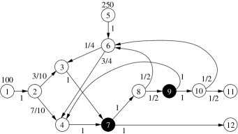
Figure 1: An emergy graph (after example of [25, p. 27]). Co-product nodes are in black. The number placed above a source node $s$ represents its weight $\theta(s)$; The number placed along an arc $(i,j)$ represents its weight $\omega_{i,j}$.

Finally, we use this partition to introduce a new definition of an emergy graph which includes functions $\theta$ and $\omega$ as weights.

Definition 2.10 (Emergy graph)

It is a weighted directed graph $(V_{s},V_{+},V_{\max},$ $V_{o},A,\theta,\omega)$ where: $V_{s}$,$V_{+}$,$V_{\max}$ and $V_{o}$ are the sets of source nodes, split nodes, co-products nodes and output nodes, respectively; $A$ is the set of arcs; $\theta(s)$ is the (nonnegative) weight of source node $s$; $\omega_{i,j}$ si the (nonnegative) weight of arc $(i,j)$;

2.3 The Maximum Empower Problem

Lahlou and Truffet [23] proved that the recursive definition of the emergy given in [26] (and expressed by eq. 5) is equivalent to a combinatorial optimization problem called the Maximum Empower Problem. To establish this result, they showed that only some paths are taken into account for computing the emergy flowing on an arc. For that, they introduced the notions of compatible paths and emergy state.

Definition 2.11 (Compatible paths)

Let $\pi=(l_{1},l_{2},\ldots,l,l^{\prime})$ and $\pi^{\prime}=(l_{1}^{\prime},l_{2}^{\prime},$ $\ldots,l,l^{\prime})$ be two paths ending by an arc $(l,l^{\prime})$. They are compatible relatively to the arc $(l,l^{\prime})$, which is denoted by $\pi\hat{+}\pi^{\prime}$, if and only if one of the following cases occurs:
(i). $\pi=\pi^{\prime}$.
(ii). $l_{1}$ and $l^{\prime}_{1}$ are two different sources.
(iii). $\exists k$, with $k\geq 1$, such that $l_{i}=l_{i}^{\prime}$, for $1\leq i\leq k$, and $l_{k}$ is a split node.

For the example given in fig. 1, paths $(3,7,8,6,4)$ and $(3,7,8,9,10,6,4)$ are compatible (case (iii) applies with $k=3$), whereas paths $(8,9,4,7)$ and $(8,9,10,6,4,7)$ are not compatible because they divide at node 9 which is a co-product.

Definition 2.12 (Emergy state)

An emergy state $\hat{\varepsilon}$, relatively to an arc $(l,l^{\prime})$, is a set of pairwise compatible emergy paths relatively to $(l,l^{\prime})$.

Using these definitions, they proved that function $\varphi$ applied to an an emergy state $\hat{\varepsilon}$ verifies (see [23, Corollary 1 and Proposition 4])

$$\varphi(\hat{\varepsilon})=\sum_{\pi\in\hat{\varepsilon}}\varphi(\pi),$$ (6)

where, for a path $\pi$ (see [26, Subsection 3.3]),

$$\varphi(\pi)=\left\{\begin{array}[]{ll}0&\mbox{if }\mathsf{lg}(\pi)=-\infty\mbox{ (i.e. }\pi=\underline{0}),\\ 1&\mbox{if }\mathsf{lg}(\pi)=0\mbox{ (i.e. }\pi=\underline{1}),\\ \theta(s)\prod_{(i,j)\in\pi}\omega_{i,j}&\mbox{if }\mathsf{lg}(\pi)\geq 1\mbox{ and }\pi\mbox{ starts by a source node }s,\\ \prod_{(i,j)\in\pi}\omega_{i,j}&\mbox{if }\mathsf{lg}(\pi)\geq 1\mbox{ and }\pi\mbox{ does not start by a source}.\\ \end{array}\right.$$ (7)

Then, they proved that

$$\mathsf{Em}(l,l^{\prime})=\max_{\hat{\varepsilon}\in\hat{E}(l,l^{\prime})}\varphi(\hat{\varepsilon}),$$ (8)

where $\hat{E}(l,l^{\prime})$ (with $\hat{E}(l,l^{\prime})\subseteq\boldsymbol{2}^{\varepsilon(l,l^{\prime})}$) denotes the set of all emergy states relatively to the arc $(l,l^{\prime})$.

This leads to the following definition of the optimization problem:

Definition 2.13 (Maximum Empower Problem)

Given an emergy graph $(V_{s},$ $V_{+},V_{\max},V_{o},A,\theta,\omega)$, an arc $(l,l^{\prime})$ of $A$, and function $\varphi$ defined by eq. 7 solve

$$\max_{\hat{\varepsilon}\in\hat{E}(l,l^{\prime})}\sum_{\pi\in\hat{\varepsilon}}\varphi(\pi)$$ (9)

Example.
Let us go back to the example given in fig. 1, and let us solve the associated Maximum Empower Problem when $(l,l^{\prime})$ is set to $(4,7)$. There are 4 emergy paths from source 1: $(1,2,4,7)$, $(1,2,3,7,8,6,4,7)$, $(1,2,3,7,8,9,4,7)$ and $(1,2,3,7,8,9,10,6,4,$ $7)$. Notice that the first path is compatible with the other three paths. And there are 2 emergy paths from source 5 ($(5,6,4,7)$ and $(5,6,3,7,8,9,4,7)$) which are also compatible.

Since two emergy paths starting from different sources are compatible (case (ii) of definition 2.11), and since $\varphi$ is a nonnegative function, an optimum emergy state $\hat{\varepsilon}^{*}$ must contain the first path starting from source 1 and both paths starting from source 5, i.e. $\{(1,2,4,7),(5,6,4,7),(5,6,3,7,8,9,4,7)\}\subseteq\hat{\varepsilon}^{*}$. Since the three remaining paths starting from source 1 are not compatible, but each of them is compatible with every path of $\{(1,2,4,7),(5,6,4,7),(5,6,3,7,8,9,4,7)\}$, only one among them can belong to $\hat{\varepsilon}^{*}$. So let us compute the value of $\varphi$ for them:
- $\varphi((1,2,3,7,8,6,4,7))=100\cdot 1\cdot\frac{3}{10}\cdot 1\cdot 1\cdot\frac{1}{2}\cdot\frac{3}{4}\cdot 1=\frac{45}{4}$,
- $\varphi((1,2,3,7,8,9,4,7))=100\cdot 1\cdot\frac{3}{10}\cdot 1\cdot 1\cdot\frac{1}{2}\cdot 1\cdot 1=15$,
- $\varphi((1,2,3,7,8,9,10,6,4,7))=100\cdot 1\cdot\frac{3}{10}\cdot 1\cdot 1\cdot\frac{1}{2}\cdot 1\cdot\frac{1}{2}\cdot\frac{3}{4}\cdot 1=\frac{45}{8}$.
Hence, we deduce that $\hat{\varepsilon}^{*}=\{(1,2,4,7),(5,6,4,7),(5,6,3,7,8,9,4,7),(1,2,3,7,$ $8,9,4,7)\}$, and we get $\varphi(\hat{\varepsilon}^{*})=(100\cdot 1\cdot\frac{7}{10}\cdot 1)+(250\cdot 1\cdot\frac{3}{4}\cdot 1)+(250\cdot 1\cdot\frac{1}{4}\cdot 1\cdot 1\cdot\frac{1}{2}\cdot 1\cdot 1)+15=70+\frac{375}{2}+\frac{125}{4}+15=303.75$ sej.

3 The maximum empower problem as a maximum weighted clique in a cograph

There are numerous definitions of a cograph (see e.g. [15]). We use the following one:

Definition 3.1

A cograph is a graph that does not contain a path of four vertices as an induced subgraph.

Hence, if a cograph contains a path of the form $(a,b,c,d)$ it must contain at least one of the edges $\{a,c\}$,$\{a,d\}$ or $\{b,d\}$. We shall use this property to show that a cograph can be associated with an emergy graph. Our proof makes also use of the following definition:

Definition 3.2

Let $P$ be a set of emergy paths $\pi_{1},\ldots,\pi_{k}$ that start from the same vertex, say $i$, and end by the same arc. The longest common prefix of $P$ is the longest path $\pi$ that starts from $i$, and such that there exist $\pi^{\prime}_{1},\ldots,\pi^{\prime}_{k}$ with $\pi_{j}=\pi\pi^{\prime}_{j}$ for $1\leq j\leq k$.

Notice that this definition together with definition 2.11 imply that two emergy paths (ending by the same arc) are not compatible if and only if they start from the same source and the last vertex of their longest common prefix is a co-product.

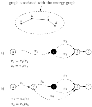
Figure 2: The argument used for showing that the set of emergy paths defines a cograph.

Theorem 1

An emergy graph and a given arc define a cograph as follows: a vertex is associated with each emergy path, and an edge is associated with each pair of vertices if they represent emergy paths that are compatible relatively to the arc.

Proof. Assume, for the sake of contradiction, that the associated graph contains a path $(a,b,c,d)$ as an induced subgraph. Let $\pi_{a},\pi_{b},\pi_{c}$ and $\pi_{d}$ be the associated emergy paths.

Since $a$ and $c$ are not joined by an edge, paths $\pi_{a}$ and $\pi_{b}$ are not compatible, that is they start from the same source and the last vertex of their longest common prefix is a co-product. Let $i$ be this vertex. Consider a decomposition into subpaths such that $\pi_{a}=\pi_{1}i\pi_{2}$ and $\pi_{c}=\pi_{1}i\pi_{3}$ (see fig. 2.a).

Since $b$ is connected to $a$ and $c$, path $\pi_{b}$ is compatible with both $\pi_{a}$ and $\pi_{c}$. Let $j$ and $j^{\prime}$ be the last vertex of the longest common prefix of $\pi_{b}$ and $\pi_{a}$, and of $\pi_{b}$ and $\pi_{c}$, respectively. Since vertices $j$ and $j^{\prime}$ are split vertices, we have $j\neq i$ and $j^{\prime}\neq i$. If $j$ belongs to $\pi_{2}$ then paths $\pi_{b}$ and $\pi_{c}$ separate at vertex $i$, i.e. $j^{\prime}=i$, which is a contradiction. Hence, $j$ belongs to $\pi_{1}$. Similarly, if $j^{\prime}$ belongs to $\pi_{3}$, we have $j=i$, which is a contradiction. Thus, $j^{\prime}$ belongs to $\pi_{1}$ and we have $j=j^{\prime}$. Let us decompose $\pi_{1}$ into $\pi_{4}j\pi_{5}$, and $\pi_{b}$ into $\pi_{4}j\pi_{6}$ (see fig. 2.b).

Now, let $k$ be the last vertex of the longest common prefix of $\pi_{b}$ and $\pi_{d}$. Since it is a co-product ($b$ and $d$ are not connected) we must have $k\neq j$, which implies that $k$ belongs to $\pi_{4}$ or $\pi_{6}$. In the former case, $k$ is also the last vertex of the longest common prefix of $\pi_{d}$ and $\pi_{c}$, which leads to a contradiction since $k$ must then be a split vertex ($d$ and $c$ are connected). In the latter case, we have again a contradiction since the last vertex of the longest common prefix of $\pi_{d}$ and $\pi_{a}$ is then vertex $j$, which implies that $d$ and $a$ are connected. Hence, vertex $k$ cannot exist, which concludes the proof.  $\Box$

Now, we are able to propose an algorithm for our problem.

Theorem 2

The Maximum Empower Problem is solved by the following algorithm:

1. Compute the set of emergy paths $\varepsilon(l,l^{\prime})$.

2. Create a graph $G$ whose sets of vertices is $\varepsilon(l,l^{\prime})$ and whose set of edges is $\{\{\pi,\pi^{\prime}\}:\pi\in\varepsilon(l,l^{\prime}),\pi^{\prime}\in\varepsilon(l,l^{\prime}),\pi\hat{+}\pi^{\prime}\}$.

3. Associate with each vertex $\pi$ of $G$ a weight equal to $\varphi(\pi)$.

4. Compute a maximum weighted clique of $G$.

Proof. By construction there is a bijection between cliques of $G$ and emergy states. Moreover, the weight of a clique $K$ is equal to $\sum_{\pi\in K}\varphi(\pi)$, which is the value of the associated emergy state (recall Definitions (6) and (7)). Since graph $G$ is a cograph (by 1) and since Jung [21] proved that a cograph is also a comparability graph, we can use the algorithm of Golumbic [19, p. 314] for finding a maximum weighted clique of a comparability graph.  $\Box$

Because Golumbic’s algorithm runs in linear time (with respect to the number of vertices and edges of the graph) and since it takes time ${\cal O}(|V_{s}\cup V_{+}\cup V_{\max}\cup V_{o}|)$ to check if two paths are compatible, the algorithm has a time complexity of ${\cal O}(|\varepsilon(l,l^{\prime})|^{2})$. Obviously, it means an exponential time in the worst case. However, we shall see in the following section that when there are no cycles, that is when the emergy graph is a directed acyclic graph (DAG), it is possible to solve the Maximum Empower Problem in polynomial time, even if there is an exponential number of emergy paths.

4 Computing the maximum empower in polyno-
mial-time when the emergy graph is a DAG

Let $G$ be an emergy graph defined by $(V_{s},V_{+},V_{\max},V_{o},A,$ $\theta,\omega)$, and let $(l,l^{\prime})\in A$. When $G$ is a DAG a path from a source to the arc $(l,l^{\prime})$ is always a simple path, which means that it is also an emergy path. Our approach is based on this remark.

Let $\varepsilon_{i}$ denote the set of simple paths starting from $i$ and ending by $(l,l^{\prime})$, and let $\hat{E}_{i}=\{\hat{e}:\hat{e}\subseteq\varepsilon_{i}\mbox{ and }\forall\pi\in\hat{e},\forall\pi^{\prime}\in\hat{e},\pi\hat{+}\pi^{\prime}\}$.

The algorithm is based on the function $f$ defined for every node $i$ of $G$ as follows:

• If $i$ is a node such that $\varepsilon_{i}=\emptyset$ then

  $$f(i)=0,$$ (10)

• else

  $$f(i)=\left\{\begin{array}[]{ll}\theta(i)&\mbox{ if }i=l\mbox{ and }i\in V_{s},\\ \omega_{i,l^{\prime}}&\mbox{ if }i=l\mbox{ and }i\notin V_{s},\\ \theta(i)f(\mathsf{succ}(i))&\mbox{ if }i\neq l\mbox{ and }i\in V_{s},\\ \sum_{j\in\Gamma^{+}(i)}\omega_{i,j}f(j)&\mbox{ if }i\neq l\mbox{ and }i\in V_{+},\\ \max_{j\in\Gamma^{+}(i)}f(j)&\mbox{ if }i\neq l\mbox{ and }i\in V_{\max}.\\ \end{array}\right.$$ (11)

It solves a particular maximization problem:

Lemma 1

Given an arc $(l,l^{\prime})$ of the emergy graph and a vertex $i$ we have

$$\max_{\hat{e}\in\hat{E}_{i}}\sum_{\pi\in\hat{e}}\varphi(\pi)=f(i)$$ (12)

Proof. If $\varepsilon_{i}=\emptyset$, then no path that starts from $i$ can end by arc $(l,l^{\prime})$. Hence, $\hat{E}_{i}=\emptyset$, so $\max_{\hat{e}\in\hat{E}_{i}}\sum_{\pi\in\hat{e}}\varphi(\pi)=\varphi(\underline{0})$, i.e. $\max_{\hat{e}\in\hat{E}_{i}}\sum_{\pi\in\hat{e}}\varphi(\pi)=0$ by (7), and relation (12) is true.

So assume that $\varepsilon_{i}\neq\emptyset$ and let us prove (12) by induction on the length $\mathsf{lg}(\pi)$ of a longest path $\pi$ of $\varepsilon_{i}$. Since $\varepsilon_{i}\neq\emptyset$, any path of $\varepsilon_{i}$ contains at least arc $(l,l^{\prime})$, which means that $\max_{\pi\in\varepsilon_{i}}\mathsf{lg}(\pi)\geq 1$ .

If $\max_{\pi\in\varepsilon_{i}}\mathsf{lg}(\pi)=1$, then $i=l$ and $\hat{E}_{i}=\{(i,l^{\prime})\}$, so $\max_{\hat{e}\in\hat{E}_{i}}\sum_{\pi\in\hat{e}}\varphi(\pi)=\varphi((i,l^{\prime}))$. If $i\in V_{s}$, $\max_{\hat{e}\in\hat{E}_{i}}\sum_{\pi\in\hat{e}}\varphi(\pi)=\theta(i)\omega_{i,l^{\prime}}$ by Definition (7) of $\varphi$, i.e. $\max_{\hat{e}\in\hat{E}_{i}}\sum_{\pi\in\hat{e}}\varphi(\pi)=\theta(i)$ since $i$ is a source (recall definition of $\omega$). Else, $\max_{\hat{e}\in\hat{E}_{i}}$ $\sum_{\pi\in\hat{e}}\varphi(\pi)=\omega_{i,l^{\prime}}$ by Definition (7) of $\varphi$. Thus, (12) is true.

If $\max_{\pi\in\varepsilon_{i}}\mathsf{lg}(\pi)\geq 2$ then $i\neq l$. Assume that for any $i$ such that $\max_{\pi\in\varepsilon_{i}}\mathsf{lg}(\pi)$ $\leq k$, with $k\geq 1$, we have $f(i)=\max_{\hat{e}\in\hat{E}_{i}}$ $\sum_{\pi\in\hat{e}}\varphi(\pi)$. Let us consider a vertex $i$ such that $\max_{\pi\in\varepsilon_{i}}\mathsf{lg}(\pi)=k+1$. We have three cases:

Case 1:

$i\in V_{s}$. Since a source has only one successor we have $\hat{e}\in\hat{E}_{i}$ if and only if there exists $\hat{e}^{\prime}$ such that $\hat{e}^{\prime}\in\hat{E}_{\mathsf{succ}(i)}$ and $\hat{e}=\{(i,\mathsf{succ}(i))\pi^{\prime}:\pi^{\prime}\in\hat{e}^{\prime}\}$. Thus, we have

$$\max_{\hat{e}\in\hat{E}_{i}}\sum_{\pi\in\hat{e}}\varphi(\pi)=\max_{\hat{e}^{\prime}\in\hat{E}_{\mathsf{succ}(i)}}\sum_{\pi^{\prime}\in\hat{e}^{\prime}}\varphi((i,\mathsf{succ}(i))\pi^{\prime}),$$

i.e., by Definition (7) of $\varphi$,

$$\max_{\hat{e}\in\hat{E}_{i}}\sum_{\pi\in\hat{e}}\varphi(\pi)=\max_{\hat{e}^{\prime}\in\hat{E}_{\mathsf{succ}(i)}}\sum_{\pi^{\prime}\in\hat{e}^{\prime}}\varphi((i,\mathsf{succ}(i)))\varphi(\pi^{\prime}).$$

Since $i\in V_{s}$, we have $\varphi((i,\mathsf{succ}(i)))=\theta(i)$ (by Definition (7) of $\varphi$) and, since $\theta(i)\geq 0$, we get

$$\max_{\hat{e}\in\hat{E}_{i}}\sum_{\pi\in\hat{e}}\varphi(\pi)=\theta(i)\max_{\hat{e}^{\prime}\in\hat{E}_{\mathsf{succ}(i)}}\sum_{\pi^{\prime}\in\hat{e}^{\prime}}\varphi(\pi^{\prime}).$$

Because $\mathsf{lg}(\pi^{\prime})\leq k$, for $\pi^{\prime}\in\hat{e}^{\prime}$, the hypothesis of induction applies, so

$$\max_{\hat{e}\in\hat{E}_{i}}\sum_{\pi\in\hat{e}}\varphi(\pi)=\theta(i)f(\mathsf{succ}(i)).$$

We conclude that (12) is true.

Case 2:

$i\in V_{+}$. If $i$ has only one successor the reasoning of Case 1 applies and (12) is true. So let us assume that $i$ has more than one successor and assume, without loss of generality, that $\Gamma^{+}(i)=\{1,\ldots,\gamma\}$ where $\gamma=|\Gamma^{+}(i)|$.

Let $j$ and $j^{\prime}$ be two successors of $i$, and let $\hat{e}\in\hat{E}_{j}$ and $\hat{e}^{\prime}\in\hat{E}_{j^{\prime}}$. Since $i$ is a split, every path of $\{(i,j)\pi:\pi\in\hat{e}\}$ is compatible with every path of $\{(i,j^{\prime})\pi^{\prime}:\pi^{\prime}\in\hat{e}^{\prime}\}$. Therefore, $\hat{e}\in\hat{E}_{i}$ if and only if there exist $\hat{e}_{j}\in\hat{E}_{j}\cup\{\emptyset\}$, for $1\leq j\leq\gamma$, such that $\hat{e}=\cup_{j=1}^{\gamma}\{(i,j)\pi_{j}:\pi_{j}\in\hat{e}_{j}\}$. Recalling that $\emptyset\notin\hat{E}_{i}$ (since $\varepsilon_{i}\neq\emptyset$) and setting $E=(\hat{E}_{1}\cup\{\emptyset\})\times\cdots\times(\hat{E}_{\gamma}\cup\{\emptyset\})\backslash(\emptyset,\ldots,\emptyset)$, we have

$$\max_{\hat{e}\in\hat{E}_{i}}\sum_{\pi\in\hat{e}}\varphi(\pi)=\max_{(\hat{e}_{1},\ldots,\hat{e}_{\gamma})\in E}\sum_{\pi\in\cup_{j=1}^{\gamma}\{(i,j)\pi_{j}:\pi_{j}\in\hat{e}_{j}\}}\varphi(\pi).$$

Since $\hat{e}_{j}\cap\hat{e}_{j^{\prime}}=\emptyset$, for $1\leq j<j^{\prime}\leq\gamma$, we get

$$\max_{\hat{e}\in\hat{E}_{i}}\sum_{\pi\in\hat{e}}\varphi(\pi)=\max_{(\hat{e}_{1},\ldots,\hat{e}_{\gamma})\in E}\sum_{1\leq j\leq\gamma}\ \sum_{\pi_{j}\in\hat{e}_{j}}\varphi((i,j)\pi_{j}),$$

i.e., by Definition (7) of $\varphi$,

$$\max_{\hat{e}\in\hat{E}_{i}}\sum_{\pi\in\hat{e}}\varphi(\pi)=\max_{(\hat{e}_{1},\ldots,\hat{e}_{\gamma})\in E}\sum_{1\leq j\leq\gamma}\ \omega_{i,j}\sum_{\pi_{j}\in\hat{e}_{j}}\varphi(\pi_{j}).$$

Applying the distributivity of operator + over $\max$ we get

$$\max_{\hat{e}\in\hat{E}_{i}}\sum_{\pi\in\hat{e}}\varphi(\pi)=\sum_{1\leq j\leq\gamma}\max_{\hat{e}_{j}\in\hat{E}_{j}\cup\emptyset}\omega_{i,j}\sum_{\pi_{j}\in\hat{e}_{j}}\varphi(\pi_{j}).$$

Since $\omega_{i,j}\geq 0$, for $(i,j)\in A$, we obtain

$$\max_{\hat{e}\in\hat{E}_{i}}\sum_{\pi\in\hat{e}}\varphi(\pi)=\sum_{1\leq j\leq\gamma}\omega_{i,j}\max_{\hat{e}_{j}\in\hat{E}_{j}\cup\emptyset}\sum_{\pi_{j}\in\hat{e}_{j}}\varphi(\pi_{j}).$$

Finally, since $\varphi(\{\emptyset\})=0$ and $\varphi\geq 0$, it is equivalent to

$$\max_{\hat{e}\in\hat{E}_{i}}\sum_{\pi\in\hat{e}}\varphi(\pi)=\sum_{1\leq j\leq\gamma}\omega_{i,j}\max_{\hat{e}_{j}\in\hat{E}_{j}}\sum_{\pi_{j}\in\hat{e}_{j}}\varphi(\pi_{j}).$$

Then, by the hypothesis of induction (which applies since $\mathsf{lg}(\pi_{j})\leq k$ for $1\leq j\leq\gamma$ and $\pi_{j}\in\hat{e}_{j}$), we obtain

$$\max_{\hat{e}\in\hat{E}_{i}}\sum_{\pi\in\hat{e}}\varphi(\pi)=\sum_{1\leq j\leq\gamma}\omega_{i,j}f(j).$$

Hence, (12) is true.

Case 3:

$i\in V_{\max}$. When $i$ has only one successor relation (12) is true because the reasoning of Case 1 applies. So let us assume that $i$ has more than one successor.

Let $j$ and $j^{\prime}$ be two successors of $i$, and let $\hat{e}\in\hat{E}_{j}$ and $\hat{e}^{\prime}\in\hat{E}_{j^{\prime}}$. Since $i$ is a co-product there is no path of $\{(i,j)\pi:\pi\in\hat{e}\}$ that can be compatible with a path of $\{(i,j^{\prime})\pi^{\prime}:\pi^{\prime}\in\hat{e}^{\prime}\}$. Therefore, we have $\hat{e}\in\hat{E}_{i}$ if and only if there exists some $\hat{e}^{\prime}$ such that $\hat{e}^{\prime}\in\hat{E}_{j}$ and $\hat{e}=\{(i,j)\pi^{\prime}:\pi^{\prime}\in\hat{e}^{\prime}\}$. Also, since $\omega_{i,j}=1$ we have $\sum_{\pi\in\hat{e}}\varphi(\pi)=\sum_{\pi^{\prime}\in\hat{e}^{\prime}}\varphi(\pi^{\prime})$ and we get

$$\max_{\hat{e}\in\hat{E}_{i}}\sum_{\pi\in\hat{e}}\varphi(\pi)=\max_{\{\hat{e}^{\prime}:\hat{e}^{\prime}\in\hat{E}_{j},j\in\Gamma^{+}(i)\}}\sum_{\pi^{\prime}\in\hat{e}^{\prime}}\varphi(\pi^{\prime}),$$

i.e.

$$\max_{\hat{e}\in\hat{E}_{i}}\sum_{\pi\in\hat{e}}\varphi(\pi)=\max_{j\in\Gamma^{+}(i)}\max_{\hat{e}^{\prime}\in\hat{E}_{j}}\sum_{\pi^{\prime}\in\hat{e}^{\prime}}\varphi(\pi^{\prime}).$$

Since, we have $\mathsf{lg}(\pi^{\prime})\leq k$ for $\pi^{\prime}\in\hat{e}^{\prime}$, the hypothesis of induction implies

$$\max_{\hat{e}\in\hat{E}_{i}}\sum_{\pi\in\hat{e}}\varphi(\pi)=\max_{j\in\Gamma^{+}(i)}f(j),$$

and we deduce that (12) is true.

$\Box$

Theorem 3

The Maximum Empower Problem can be solved in time $\Theta(|V_{s}\cup V_{+}\cup V_{\max}\cup V_{o}|+|A|)$ when the emergy graph is a DAG, and the optimal value is obtained by

$$\mathsf{Em}(l,l^{\prime})=\sum_{s\in V_{s}}f(s),$$ (13)

where $f$ is defined by (11).

Proof. By eq. 6 and eq. 8 we have $\mathsf{Em}(l,l^{\prime})=\max_{\hat{\varepsilon}\in\hat{E}(l,l^{\prime})}\sum_{\pi\in\hat{\varepsilon}}\varphi(\pi)$. By definition, $\hat{E}(l,l^{\prime})$ is the set of all emergy states relatively to arc $(l,l^{\prime})$. Recalling that an emergy state is a set of pairwise compatible emergy paths, and that paths starting from different sources are always compatible (case (ii) of definition 2.11), we have $\hat{\varepsilon}\in\hat{E}(l,l^{\prime})$ if and only if there exist $\hat{\varepsilon}_{s}$, with $s\in V_{s}$, such that $\hat{\varepsilon}_{s}\in\hat{E}_{s}$ and $\hat{\varepsilon}=\cup_{s\in V_{s}}\hat{\varepsilon}_{s}$. Without loss of generality, we assume that $V_{s}=\{1,\ldots,\gamma\}$ where $\gamma=|V_{s}|$.

The reasoning is then almost the same as for Case 2 of 1. Setting $E=\hat{E}_{1}\times\cdots\times\hat{E}_{\gamma}$, we have

$$\max_{\hat{\varepsilon}\in\hat{E}(l,l^{\prime})}\sum_{\pi\in\hat{\varepsilon}}\varphi(\pi)=\max_{(\hat{\varepsilon}_{1},\ldots,\hat{\varepsilon}_{\gamma})\in E}\sum_{\pi_{j}\in\cup_{j=1}^{\gamma}\hat{\varepsilon}_{j}}\varphi(\pi_{j}).$$

Since $\hat{\varepsilon}_{j}\cap\hat{\varepsilon}_{j^{\prime}}=\emptyset$, for $1\leq j<j^{\prime}\leq\gamma$, we get

$$\max_{\hat{\varepsilon}\in\hat{E}(l,l^{\prime})}\sum_{\pi\in\hat{\varepsilon}}\varphi(\pi)=\max_{(\hat{\varepsilon}_{1},\ldots,\hat{\varepsilon}_{\gamma})\in E}\sum_{1\leq j\leq\gamma}\ \sum_{\pi_{j}\in\hat{\varepsilon}_{j}}\varphi(\pi_{j}).$$

Applying the distributivity of operator + over $\max$ we get

$$\max_{\hat{\varepsilon}\in\hat{E}(l,l^{\prime})}\sum_{\pi\in\hat{\varepsilon}}\varphi(\pi)=\sum_{1\leq j\leq\gamma}\max_{\hat{\varepsilon}_{j}\in\hat{E}_{j}}\sum_{\pi_{j}\in\hat{\varepsilon}_{j}}\varphi(\pi_{j}).$$

By 1 we have $f(j)=\max_{\hat{\varepsilon}\in\hat{E}_{j}}\sum_{\pi\in\hat{\varepsilon}}\varphi(\pi)$, for $1\leq j\leq\gamma$. Thus, $\mathsf{Em}(l,l^{\prime})=\sum_{s\in V_{s}}f(s)$, which completes the proof.

Now, let us prove the time complexity. Let $V=V_{s}\cup V_{+}\cup V_{\max}\cup V_{o}$. First, we determine, for every $i$ of $V$, if $\hat{\varepsilon}_{i}=\emptyset$ or $\hat{\varepsilon}_{i}\neq\emptyset$, i.e. if node $l$ is reachable from node $i$. To do so, it suffices to compute the shortest paths from $l$ to every node $i$ in the graph $G$ where each arc is reversed. This can be done in $\Theta(|V|+|A|)$ (see, e.g., [14, p. 655]) by computing a topological order $L$ for the vertices of $V$ (i.e. if $(i_{j},i_{k})$ is an arc then vertex $i_{j}$ is before $i_{k}$ in $L$).

Second, we compute $f(i)$ by considering elements $i$ of $V$ in the order of $L$: formula (11) is applied $|\Gamma^{+}(i)|$ times for every $i$, which leads to a total time of $\Theta(|V|+|A|)$.

Finally, computing the sum $\sum_{s\in V_{s}}f(s)$ takes time $\Theta(|V_{s}|)$, so the overall time complexity is $\Theta(|V|+|A|)$.  $\Box$

When the emergy graph is a DAG the time-complexity of the Maximum Empower Problem does not depend on the number of emergy paths. But, in the general case, is it possible to avoid an exponential-time complexity, contrary to the algorithm proposed in section 3? We answer the question in the following section.

5 Hardness of computing the maximum empower in the general case

The Maximum Empower Problem does not seem to belong to NP since we do not know how to provide a certificate that can be checked in polynomial time. However, the difficulty of computing is clearly based on the set $\varepsilon(l,l^{\prime})$ of emergy paths, which are simple paths when node $l^{\prime}$ is not repeated. Valiant [43] proved that the problem of counting the number of simple paths between two vertices of a directed graph is a #P-complete problem. We prove that Valiant’s problem can be solved in polynomial time by a nondeterministic Turing machine equipped with an oracle for the Maximum Empower Problem.

Figure 3: The reduction used to prove the #P-hardness of the Maximum Empower Problem.

Theorem 4

The Maximum Empower Problem is #P-hard.

Proof. Let $G^{\prime}=(V^{\prime},A^{\prime},s^{\prime},t^{\prime})$ be an instance of the problem of counting the number of simple paths between two vertices of a directed graph, where $s^{\prime}$ and $t^{\prime}$ are the start and target vertices, respectively. Since the number of paths from $s^{\prime}$ to $t^{\prime}$ that have $i$ vertices is bounded by $\frac{|V^{\prime}|!}{(|V^{\prime}|-i)!}$, the value $B=\sum_{i=1}^{|V^{\prime}|}\frac{|V^{\prime}|!}{(|V^{\prime}|-i)!}$ is an upper bound on the number of simple paths from $s^{\prime}$ to $t^{\prime}$. We transform this instance into a Maximum Empower Problem instance as follows (see fig. 3):

1. $V_{s}=\{s\}$, $V_{+}=V^{\prime}$, $V_{\max}=\emptyset$, and $V_{o}=\{t,u\}$.

2. $A=A^{\prime}\cup\{(s,s^{\prime}),(t^{\prime},t)\}\cup\{(i,u):i\in V^{\prime}\cup\{s^{\prime}\}\}$.

3. $\omega_{i,j}=\frac{1}{B}$ for $(i,j)\in A^{\prime}$.

4. $\omega_{i,u}=1-\frac{|\Gamma^{+}(i)|}{B}$ for $i\in V^{\prime}\cup\{s^{\prime}\}$.

5. $\omega_{s,s^{\prime}}=1$ and $\omega_{t^{\prime},t}=1-\frac{|\Gamma^{+}(t^{\prime})|}{B}$.

6. $\theta(s)=1$.

Notice that we have $\sum_{j\in\Gamma^{+}(i)}\omega_{i,j}=1$ for $i\in V_{+}$, which is required for an emergy graph (recall definition of $\omega$).

We first call the oracle to get the value of $\mathsf{Em}(t^{\prime},l)$. Since there are no co-product nodes, any set of emergy paths is an emergy state. By (8) and because $\varphi(\pi)\geq 0$, for an emergy path $\pi$, we deduce that $\mathsf{Em}(t^{\prime},t)=\sum_{\pi\in\hat{E}(t^{\prime},l)}\varphi(\pi)$, where $\hat{E}(t^{\prime},t)$ is the set of all emergy paths ending by arc $(t^{\prime},t)$.

Then, we use this value to find the number of simple paths from $s^{\prime}$ to $t^{\prime}$. Let $n_{i}$ be the number of elements of $\hat{E}(t^{\prime},t)$ of length $i$, i.e. of emergy paths that have exactly $i$ arcs. For such a path $\pi$ we get $\varphi(\pi)=\theta(s)\omega_{s,s^{\prime}}(\frac{1}{B})^{i-2}\omega_{t^{\prime},t}=\frac{1}{B^{i-2}}\omega_{t^{\prime},t}$. Hence, we have $\mathsf{Em}(t^{\prime},t)=\sum_{i=2}^{i=|V^{\prime}|+1}\frac{n_{i}}{B^{i-2}}\omega_{t^{\prime},t}$, since $2\leq i\leq|V^{\prime}|+1$.

Now, let $E^{\prime}=\frac{\mathsf{Em}(t^{\prime},t)}{w_{t^{\prime},t}}$. Since $n_{i}<B$ (by construction), we can retrieve the value of the $n_{i}$’s from $E^{\prime}$ by considering the representation of $E^{\prime}$ in basis $\frac{1}{B}$: by multiplying $E^{\prime}$ by $B$ and taking the integer part we get $n_{2}$; if we substract $n_{2}$ to $E^{\prime}$ and repeat the process we get $n_{3}$, and so on. Hence, we can get the value $\sum_{i=2}^{i=|V^{\prime}|+1}n_{i}$, which is the number of simple paths from $s$ to $t$.

Since both the transformation and the computation of $\sum_{i=2}^{i=|V^{\prime}|+1}n_{i}$ can be done in polynomial time, we deduce the #P-hardness of our problem. $\Box$

6 Conclusion

We have proved that the Maximum Empower Problem is #P-hard, but solvable in polynomial-time when the emergy graph has no cycles. However, taking into account cycles is not only a theoretical problem because feedback arcs in the emergy graph model recycling processes, which are part of numerous real systems. If there are cycles and the number of emergy paths is a polynomial of the size of the emergy graph, we can solve the problem in polynomial time by using the algorithm we have provided for the general case. These remarks raise the following question: Q1: Is there a kind of emergy graph with cycles and an exponential number of emergy paths for which the Maximum Empower Problem can be solved in polynomial time?

A second question is related to the type of nodes in the emergy graphs, i.e. split or co-products. Indeed, since no co-product nodes are used in the reduction of the proof of #P-hardness, the complexity of the problem seems to rely on the existence of split nodes (and cycles of course). Moreover, in case of an emergy graph with no split nodes the problem is trivially solvable: only one emergy path per source can belong to an emergy state, and the weights are all equal to 1; Hence, the problem reduces to finding a simple path from each source to the arc $(l,l^{\prime})$, and the optimal value is then simply the value $\sum_{\{s:\mbox{ there is a path from }s\mbox{ to }(l,l^{\prime})\}}\theta(s)$. This suggests the following problem: Q2: What is the complexity of the Maximum Empower Problem when the number of split nodes is fixed?

References

- [1] F. Baccelli, G. Cohen, G.J. Olsder, and J-P. Quadrat. Synchronization and Linearity. John Wiley and Sons, 1992.
- [2] R. C. Backhouse and B. A. Carré. Regular algebra applied to path-finding problems. IMA Journ Appl. Math, 15(2), 1975. (161-186).
- [3] E. Bardi, M.J. Cohen, and M. T. Brown. A Linear Optimization Method for Computing Transformities from Ecosystem Energy Webs. Emergy synthesis 3: theory and applications of the emergy methodologies, 2005. (63-74).
- [4] S. Bastianoni, F. Morandini, T. Flaminio, R. M. Pulselli, and E. B. P. Tiezzi. Emergy and Emergy Algebra Explained by Means of Ingenuous Set Theory. Ecological Modelling, 222, 2011. (2903-2907).
- [5] C. Benzaken. Structures Algébriques des Cheminements: Pseudo-Treillis, Gerbiers de Carré Nul. in Network and Switching Theory, 1968. (40-57).
- [6] L. Boltzmann. Der Zweite Hauptsatz der Mechanischen Wärmetheorie. 1886.
- [7] M. T. Brown, D. E. Campbell, C. De Vilbiss, and S. Ulgiati. The Geobiosphere Emergy Baseline: A Synthesis. Ecol. Model., 339, 2016. (92-95).
- [8] M. T. Brown and R. A. Herendeen. Embodied Energy Analysis and Emergy Analysis: a Comparative View. Ecological Economics, 19, 1996. (219-235).
- [9] M. T. Brown, G. Protano, and S. Ulgiati. Assessing Geobiosphere Work of Generating Global Reserves of Coal, Crude Oil, and Natural Gas . Ecological Modelling, 222(3), 2011. (879-887).
- [10] D. E. Campbell. Emergy baseline for the Earth: A historical review of the science and a new calculation. Ecol. Model., 339, 2016. (96-125).
- [11] B. A. Carré. An Algebra For Network Routing Problems. J. Inst. Math. Appl., 7, 1971. (273-294).
- [12] W. Chen, W. Liu, Y. Geng, M. T. Brown, C. Gao, and R. Wu. Recent Progress on Emergy Research: A Bibliometric Analysis. Renewable and Sustainable Energy Reviews, 73, 2017. (1051-1060).
- [13] D. Collins and H. T. Odum. Calculating Transformities With Eigenvector Method. Emergy synthesis: theory and applications of the emergy methodologies, 2000. (265-280).
- [14] Thomas H. Cormen, Charles E. Leiserson, Ronald L. Rivest, and Clifford Stein. Introduction to algorithms. The MIT Press, 3rd edition, 2009.
- [15] D. G. Corneil, H. Lerchs, and L. Stewart Burlingham. Complement reducible graphs. Discrete Applied Mathematics, 3:163–174, 1981.
- [16] C. De Vilbiss, M. T. Brown, E. Siegel, and S. Arden. Computing The Geobiosphere Emergy Baseline: A Novel Approach. Ecol. Model., 339, 2016. (133-139).
- [17] C. Giannantoni. The Maximum Empower Principle as the Basis for Thermodynamics of Quality. SG Editoriali, 2002.
- [18] C. Giannantoni. Mathematics For Generative Processes: Living and Non-living Systems. Journ. Comp. Appl. Math., 189, 2006. (324-340).
- [19] Martin Charles Golumbic. Topics on perfect graphs. In Claude Berge and Vasek Chvátal, editors, Annals of Discrete Mathematics, volume 21. North-Holland, 1984.
- [20] J.H. Horlock. Cogeneration-Combined heat and power: Thermodynamics and economics. Krieger Publishing Company, 1996.
- [21] H. A. Jung. On a class of posets and the corresponding comparability graphs. Journal of Combinatorial Theory, Series B, 24:125–133, 1978.
- [22] C. Kazanci, J. R. Schramski, and S. Bastianoni. Individual Based Emergy Analysis: A Lagrangian Model of Energy Memory. Ecological Complexity, 11, 2012. (103-108).
- [23] C. Lahlou and L. Truffet. Self-organization and the Maximum Empower Principle in the Framework of max-plus Algebra, 2017. arXiv:1712.05798.
- [24] A. Lazzaretto. A Critical Comparison Between Thermoeconomic and Emergy Analyses Algebra. Energy, 34, 2009. (2196-2205).
- [25] O. Le Corre. Emergy. ISTE PRESS, 2016.
- [26] O. Le Corre and L. Truffet. A Rigourous Mathematical Framework for Computing a Sustainability Ratio: the Emergy. Journal of Environmental Informatics, 20(2), 2012. (75-89).
- [27] O. Le Corre and L. Truffet. Exact Computation of Emergy Based on a Mathematical Reinterpretation of the Rules of Emergy Algebra. Ecological Modelling, 230, 2012. (101-113).
- [28] O. Le Corre and L. Truffet. Emergy Paths computation from Interconnected Energy System Diagram. Ecol. Model., 313, 2015. (181-200).
- [29] W. Leontief. Input-Output economics. Oxford University Press, 1973.
- [30] L. Li, H. Lu, D. E. Campbell, and H. Ren. Emergy Algebra: Improving Matrix Method for Calculating Transformities. Ecological Modelling, 221, 2010. (411-422).
- [31] A. Marvuglia, E. Benetto, B. Rugani, and G. Rios. A Scalable Implementation of the Track Summing Algorithm For Emergy Calculation With Life Cycle Inventory Databases. In EnviroInfo 2011, 2011.
- [32] A. Marvuglia, B. Rugani, G. Rios, Y. Pigné, E. Benetto, and L. Tiruta-Barna. Using graph search algorithms for a rigorous application of emergy algebra rules. Rev. Métal., 110(1), 2013. (87-94).
- [33] M. J. Moran, H. N. Shapiro, D. D. Boettner, and M. B. Bailey. Fundamentals of Engineering Thermodynamics. Wiley, 2014. 8th Edition.
- [34] H. Mu, X. Feng, and K. Hoong Chu. Calculation of Emergy Flows Within Complex Chemical Production Systems. Ecol. Engin., 44, 2012. (88-93).
- [35] H. T. Odum. Self-organization and Maximum Empower. In C. A. S. Hall (Ed.), Maximum Power: The Ideas and Applications of H. T. Odum, 1995. Colorado University Press, Colorado.
- [36] H. T. Odum. Environmental accounting. EMERGY and decision making. John Wiley, 1996.
- [37] H. T. Odum and R. C. Pinkerton. Time’s Speed Regulator: The Optimum Efficiency for Maximum Power Output in Physical and Biological Systems. American Scientist, 43(2), 1955. (331-343).
- [38] M. Patterson. Evaluation of Matrix Algebra Methods for Calculating Transformities from Ecological and Economic Network Data. Ecological Modelling, 271, 2014. (72-82).
- [39] S. Podolinsky. Le travail Humain et la Conservation de l’Energie. Rev. Intern. des Sciences, 5, 1880. (57-70).
- [40] D. M. Scienceman. Energy and Emergy. In Environmental Economics-The Analysis of a Major Interface. Pillet, G. and Murota, T. (eds.), 1987. (257-276).
- [41] S. E. Tennenbaum. Network energy expenditures for subsystem production. PhD thesis, University of Florida, Gainesville, 1988.
- [42] S. E. Tennenbaum. Emergy and Co-emergy. Ecol. Model., 2014. http://dx.doi.org/10.1016/j.ecolmodel.2014.09.012.
- [43] Leslie Valiant. The complexity of enumeration and reliability problems. SIAM Journal on Computing, 8(3):410–421, 1979.
- [44] R. Valyi. About the Emergy Concept. Technical report, Ecole Centrale de Lyon, FRANCE, 2005. http://emsim.sourceforge.net/latexdocs/emergy.pdf.
- [45] S. Zhong, Y. Geng, W. Liu, C. Gao, and W. Chen. A Bibliometric Review on Natural Resource Accounting During 1995–2014. Journ. Cleaner Prod., 139, 2016. (122-132).